average idiosyncratic volatility in g7 countries

Research Division Federal Reserve Bank of St. Louis Working Paper Series

Average Idiosyncratic Volatility in G7 Countries

Hui Guo and

Robert Savickas

Working Paper 2004-027C http://research.stlouisfed.org/wp/2004/2004-027.pdf

November 2004 Revised January 2007

FEDERAL RESERVE BANK OF ST. LOUIS Research Division

P.O. Box 442 St. Louis, MO 63166

______________________________________________________________________________________

The views expressed are those of the individual authors and do not necessarily reflect official positions of the Federal Reserve Bank of St. Louis, the Federal Reserve System, or the Board of Governors.

Federal Reserve Bank of St. Louis Working Papers are preliminary materials circulated to stimulate discussion and critical comment. References in publications to Federal Reserve Bank of St. Louis Working Papers (other than an acknowledgment that the writer has had access to unpublished material) should be cleared with the author or authors.


Hui Guoa and Robert Savickasb*

This Version: November 2006

*a Research Division, Federal Reserve Bank of St. Louis (P. O. Box 442, St. Louis, MO, 63166-0442, E-mail: [email protected]); and b Department of Finance, George Washington University (2023 G Street, N.W. Washington, DC 20052, E-mail: [email protected]). We are especially grateful to an anonymous referee and the editor, Joel Hasbrouck, for numerous insightful and constructive comments, which greatly improved the paper. We thank Andrew Ang, Torben Andersen, Samuel Thompson, Tuomo Vuolteenaho, Mathijs van Dijk, Valerio Poti, and participants at the 2005 Financial Management Association meeting in Chicago, the 2005 Southern Finance Association meeting in Key West, the 2006 Washington Area Finance Association meeting in Washington D.C., the 2006 Financial Management Association European meeting in Stockholm, and the 2006 INFINITI Conference in Dublin for helpful suggestions and discussion. We also thank Timothy Vogelsang for providing Gauss codes and Jason Higbee for excellent research assistance. The views expressed in this paper are those of the authors and do not necessarily reflect the official positions of the Federal Reserve Bank of St. Louis or the Federal Reserve System.


Abstract

We argue that changes in average idiosyncratic volatility provide a proxy for changes in

the investment opportunity set, and this proxy is closely related to the book-to-market factor. We

test this idea in two ways using G7 countries’ data. First, we show that idiosyncratic volatility

has statistically significant predictive power for aggregate stock market returns over time.

Second, we show that idiosyncratic volatility performs just as well as the book-to-market factor

in explaining the cross section of stock returns. Our results suggest that the hedge against

changes in investment opportunities is an important determinant of asset prices.

Keywords: Idiosyncratic Volatility, Stock Market Volatility, Value Premium, Stock Return

Predictability, ICAPM, Unit Root, Deterministic Trend, and Granger Causality.

JEL number: G1.

1

I. Introduction

There is an ongoing debate about whether average firm-level idiosyncratic stock return

volatility forecasts stock market returns. Using monthly U.S. data over the period July 1962 to

December 1999, Goyal and Santa-Clara (2003) report that the equal-weighted total volatility is

positively and significantly related to future stock market returns, although stock market

volatility has negligible predictive power.1 However, subsequent studies, e.g., Bali, Cakici, Yan,

and Zhang (2005) and Wei and Zhang (2005), show that neither idiosyncratic volatility nor stock

market volatility forecasts stock market returns in an extended sample ending in 2001. In

contrast, using quarterly data over the period 1963 to 2002, Guo and Savickas (2006) find that,

when combined with stock market volatility, the value-weighted idiosyncratic volatility is

negatively and significantly related to stock market returns.2 Consistent with the CAPM, Guo

and Savickas also document a positive relation between stock market volatility and returns.

In this paper, we try to shed light on this controversy by arguing that changes in

idiosyncratic volatility provide a proxy for changes in investment opportunities. Specifically, we

argue that this proxy is closely related to the book-to-market factor advocated by Fama and

French (1996). The main idea is as follows. Technological innovations—which are an important

component of a firm’s investment opportunities—have two major effects on the firm’s stock

price. First, they tend to increase the level of the firm’s stock price because of growth options.

Second, they also tend to increase the volatility of the firm’s stock price because of the

1 Campbell, Lettau, Malkiel, and Xu (2001) adopt a nonparametric approach to decompose an individual stock return into three components: a market-wide return, an industry-specific residual, and a firm-specific residual. Other authors, e.g., Bali, Cakici, Yan, and Zhang (2005), Wei and Zhang (2005), and Guo and Savickas (2006), use the CAPM or the Fama and French (1993) 3-factor model to adjust for systematic risk. In general, the results are not sensitive to any particular measure of idiosyncratic volatility because Goyal and Santa-Clara (2003) show that total stock price volatility is predominantly composed of idiosyncratic volatility. 2 Idiosyncratic volatility and stock market volatility have stronger forecasting power for stock returns in quarterly data than monthly data possibly because, as pointed out by Ghysels, Santa-Clara, and Valkanov (2005), realized volatility is a function of long distributed lags of daily returns. We also use quarterly data in this paper.

2

uncertainty about which firms will benefit from the new opportunities. That is, as confirmed by

recent empirical studies, e.g., Duffee (1995), Pastor and Veronesi (2003, 2005), Agarwal,

Bharath, and Viswanathan (2004), and Mazzucato (2002), firms that adopt new technologies

tend to have higher stock market valuations and higher stock price volatility than firms that do

not adopt new technologies. Moreover, Berk, Green, and Naik (1999) show that the valuation of

a firm’s investment opportunities depends crucially on the time-varying cost of capital. And their

model implies that the aggregate book-to-market ratio forecasts stock market returns because of

its comovements with the conditional equity premium. Therefore, because a firm’s volatility is

closely related to its investment opportunities and thus its book-to-market ratio, the average

idiosyncratic volatility is negatively related to future stock market returns possibly because of its

negative correlation with the aggregate book-to-market ratio.

We test this idea in two ways. First, we show that idiosyncratic volatility has predictive

power for aggregate stock market returns across time. For robustness, we use both U.S. data

obtained from CRSP (the Center for Research in Security Prices) and the other G7 countries’

data obtained from the Datastream. We find that, for most G7 countries, idiosyncratic volatility

and stock market volatility jointly forecast stock market returns, although neither variable has

significant predictive power individually. Moreover, U.S. idiosyncratic volatility has significant

predictive power for international stock market returns, even after we control for the local

counterparts. Similarly, because of their strong comovements with U.S. data, idiosyncratic

volatility of the other G7 countries also forecasts U.S. stock market returns.

Second, we show that idiosyncratic volatility is closely related to the book-to-market

factor. As hypothesized, in U.S. data, the relation between idiosyncratic volatility and the

aggregate book-to-market ratio is significantly negative. More importantly, we find that

3

idiosyncratic volatility performs just as well as the book-to-market factor in explaining the cross

section of stock returns on the 25 Fama and French (1993) portfolios sorted on size and the

book-to-market ratio. We also find a very similar result using the Fama and French (1998)

international value and growth portfolios.

Hamao, Mei, and Xu (2003) and Frazzini and Marsh (2003) have investigated

idiosyncratic volatility for Japan and the U.K., respectively. However, unlike this paper, those

studies focus on idiosyncratic volatility of a particular country and don’t address its commonality

across countries. Moreover, some of our results are different from theirs. For example, Hamao,

Mei, and Xu (2003) fail to reject a unit root in Japanese value-weighted idiosyncratic volatility

but it is found to be stationary here. Also, we find a significantly negative relation between the

value-weighted idiosyncratic volatility and future stock market returns for the U.K., in contrast

with the positive relation reported by Frazzini and Marsh (2003).

The remainder of the paper is organized as follows. Because we use idiosyncratic

volatility as a new risk factor, it is important to understand its statistical properties. This issue is

addressed in Section II. We investigate predictive abilities of average idiosyncratic volatility for

stock market returns and the value premium in Section III, and provide some discussion as well

as additional evidence in Section IV. Some concluding remarks are offered in Section V.

II. Data

We obtain daily value-weighted stock market return and daily individual stock return data

for the U.S. over the period July 1962 to December 2003 from the CRSP database. We obtain the

same variables denominated in local currencies over the period January 1965 to December 2003

for the U.K. and over the period January 1973 to December 2003 for Canada, France, Germany,

4

Italy, and Japan from the Datastream. As in Campbell, Lettau, Malkiel, and Xu (2001), we

assume that the daily risk-free rate is the rate which, over the number of calendar days,

compounds to the monthly T-bill rate. The monthly T-bill rate is obtained from IFS

(International Financial Statistics) for all countries.

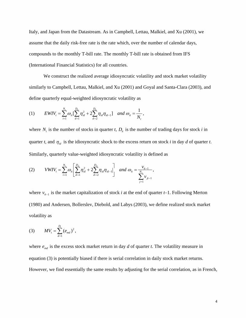
We construct the realized average idiosyncratic volatility and stock market volatility

similarly to Campbell, Lettau, Malkiel, and Xu (2001) and Goyal and Santa-Clara (2003), and

define quarterly equal-weighted idiosyncratic volatility as

(1) 21

1 1 2

1[ 2 ]t it itN D D

t it id id id iti d d t

EWIV andN

ω η η η ω−= = =

= + =∑ ∑ ∑ ,

where Nt is the number of stocks in quarter t, Dit is the number of trading days for stock i in

quarter t, and idη is the idiosyncratic shock to the excess return on stock i in day d of quarter t.

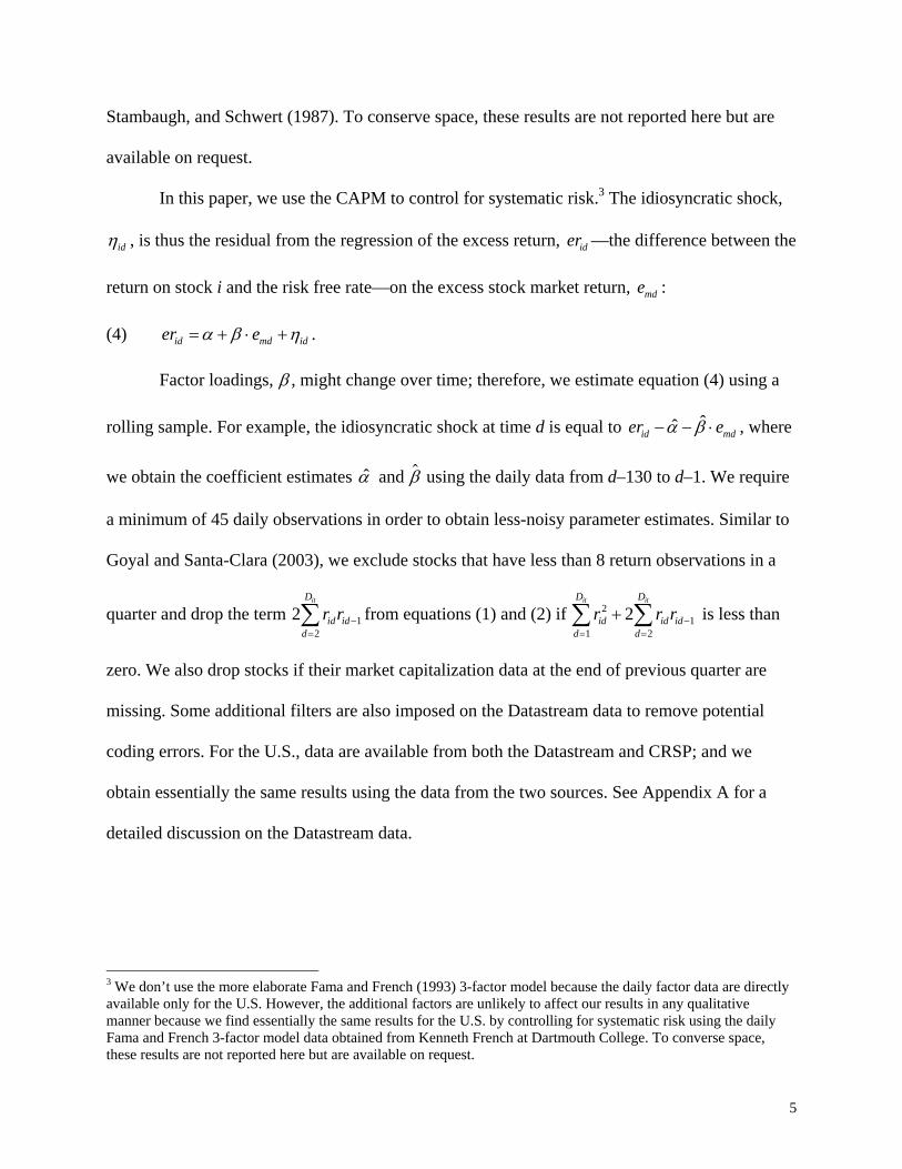
Similarly, quarterly value-weighted idiosyncratic volatility is defined as

(2) ,2

11

1

1 21

1

2

∑∑ ∑∑

=−

−

= =−

=

=⎥⎦

⎤⎢⎣

⎡+=

t

t itit

N

jjt

itit

N

i

D

didid

D

diditt

v

vandVWIV ωηηηω

where vit−1 is the market capitalization of stock i at the end of quarter t–1. Following Merton

(1980) and Andersen, Bollerslev, Diebold, and Labys (2003), we define realized stock market

volatility as

(3) 2

1( )

tD

t mdd

MV e=

= ∑ ,

where emd is the excess stock market return in day d of quarter t. The volatility measure in

equation (3) is potentially biased if there is serial correlation in daily stock market returns.

However, we find essentially the same results by adjusting for the serial correlation, as in French,

5

Stambaugh, and Schwert (1987). To conserve space, these results are not reported here but are

available on request.

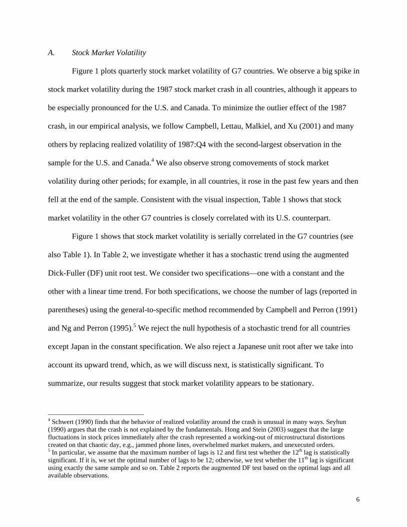
In this paper, we use the CAPM to control for systematic risk.3 The idiosyncratic shock,

idη , is thus the residual from the regression of the excess return, ider —the difference between the

return on stock i and the risk free rate—on the excess stock market return, mde :

(4) id md ider eα β η= + ⋅ + .

Factor loadings, β , might change over time; therefore, we estimate equation (4) using a

rolling sample. For example, the idiosyncratic shock at time d is equal to ˆˆid mder eα β− − ⋅ , where

we obtain the coefficient estimates α̂ and β using the daily data from d–130 to d–1. We require

a minimum of 45 daily observations in order to obtain less-noisy parameter estimates. Similar to

Goyal and Santa-Clara (2003), we exclude stocks that have less than 8 return observations in a

quarter and drop the term 2 12

r rid idd

Dit

−=∑ from equations (1) and (2) if r r rid

d

D

id idd

Dit it2

11

2

2+=

−=

∑ ∑ is less than

zero. We also drop stocks if their market capitalization data at the end of previous quarter are

missing. Some additional filters are also imposed on the Datastream data to remove potential

coding errors. For the U.S., data are available from both the Datastream and CRSP; and we

obtain essentially the same results using the data from the two sources. See Appendix A for a

detailed discussion on the Datastream data.

3 We don’t use the more elaborate Fama and French (1993) 3-factor model because the daily factor data are directly available only for the U.S. However, the additional factors are unlikely to affect our results in any qualitative manner because we find essentially the same results for the U.S. by controlling for systematic risk using the daily Fama and French 3-factor model data obtained from Kenneth French at Dartmouth College. To converse space, these results are not reported here but are available on request.

6

A. Stock Market Volatility

Figure 1 plots quarterly stock market volatility of G7 countries. We observe a big spike in

stock market volatility during the 1987 stock market crash in all countries, although it appears to

be especially pronounced for the U.S. and Canada. To minimize the outlier effect of the 1987

crash, in our empirical analysis, we follow Campbell, Lettau, Malkiel, and Xu (2001) and many

others by replacing realized volatility of 1987:Q4 with the second-largest observation in the

sample for the U.S. and Canada.4 We also observe strong comovements of stock market

volatility during other periods; for example, in all countries, it rose in the past few years and then

fell at the end of the sample. Consistent with the visual inspection, Table 1 shows that stock

market volatility in the other G7 countries is closely correlated with its U.S. counterpart.

Figure 1 shows that stock market volatility is serially correlated in the G7 countries (see

also Table 1). In Table 2, we investigate whether it has a stochastic trend using the augmented

Dick-Fuller (DF) unit root test. We consider two specifications—one with a constant and the

other with a linear time trend. For both specifications, we choose the number of lags (reported in

parentheses) using the general-to-specific method recommended by Campbell and Perron (1991)

and Ng and Perron (1995).5 We reject the null hypothesis of a stochastic trend for all countries

except Japan in the constant specification. We also reject a Japanese unit root after we take into

account its upward trend, which, as we will discuss next, is statistically significant. To

summarize, our results suggest that stock market volatility appears to be stationary.

4 Schwert (1990) finds that the behavior of realized volatility around the crash is unusual in many ways. Seyhun (1990) argues that the crash is not explained by the fundamentals. Hong and Stein (2003) suggest that the large fluctuations in stock prices immediately after the crash represented a working-out of microstructural distortions created on that chaotic day, e.g., jammed phone lines, overwhelmed market makers, and unexecuted orders. 5 In particular, we assume that the maximum number of lags is 12 and first test whether the 12th lag is statistically significant. If it is, we set the optimal number of lags to be 12; otherwise, we test whether the 11th lag is significant using exactly the same sample and so on. Table 2 reports the augmented DF test based on the optimal lags and all available observations.

7

Lastly, consistent with the early studies, e.g., Schwert (1989), Figure 1 shows that there is

no trend in U.S. stock market volatility over the post-World War II sample. Similarly, we find no

obvious trend for Canada, France, Italy, or the U.K. However, stock market volatility appears to

have increased substantially for Germany and Japan over the period 1973 to 2003. In Table 3, we

formally investigate this issue using Vogelsang’s (1998) PS1 test.6 Consistent with Figure 1, we

find a significant upward trend in stock market volatility for Germany and Japan but not the

other countries. Our results are not specific to the Datastream data because we obtain the same

conclusion using the MSCI (Morgan Stanley Capital International) daily market return data.7 The

existing literature provides no explanation for the puzzling upward trend; however, a formal

investigation is beyond the scope of this paper and we leave it for future research.

B. Idiosyncratic Volatility

Figure 2 plots the equal-weighted idiosyncratic volatility (thin line) along with the value-

weighted idiosyncratic volatility (thick line).8 We observe strong comovements in both measures

of idiosyncratic volatility across countries. For example, it rose sharply around the late 1990s and

then fell steeply afterward. It is also interesting to note that, in contrast with stock market

volatility, the 1987 stock market crash has a relatively small effect on idiosyncratic volatility.

Consistent with the visual inspection, Table 1 shows that idiosyncratic volatility in the other G7

6 Vogelsang (1998) shows that the PS1 test has good size properties and is valid even in the presence of nonstationarity. Moreover, it also has good power properties for stationary variables. Nevertheless, our main results are qualitatively unchanged in various tests discussed in Vogelsang (1998). 7 Hamao, Mei, and Xu (2003) also document an upward trend in Japanese stock market volatility. 8 Before 1989, the Datastream includes only Toronto Stock Exchange issues for Canada; however, it also includes firms listed on the Vancouver Stock Exchange afterward. As a result, the number of stocks used in our calculation increases sharply from 345 in the last quarter of the year 1988 to 743 in the first quarter of the year 1989. Because the Vancouver Stock Exchange had a lot of small and highly risky natural resource exploration stocks (see, e.g. "Scam capital of the world" Forbes, May 29 1989), the inclusion of Vancouver stocks dramatically raises the equal-weighted idiosyncratic volatility for Canada but has small effects on the value-weighted measure.

8

countries, both value- (panel A) and equal-weighted (panel B), is highly correlated with its U.S.

counterpart. To our best knowledge, this result has not been reported elsewhere.

We also investigate in Table 2 whether idiosyncratic volatility has a stochastic trend.

Consistent with the early authors, e.g., Campbell, Lettau, Malkiel, and Xu (2001), we reject the

null hypothesis of a unit root in U.S. value-weighted idiosyncratic volatility at the 5 percent

significance level in the constant specification. We also reject the unit root in the value-weighted

idiosyncratic volatility at the 1 percent significance level for Japan, the 5 percent level for the

U.K., and the 10 percent level for Germany and Italy.9 We find similar results in the trend

specification, although the evidence against the unit root is somewhat weaker than in the

constant specification. The latter result reflects the fact that the trend specification has less power

because, as we will show below, we find no deterministic trend in the value-weighted

idiosyncratic volatility of all G7 countries. In contrast, the evidence against the unit root is much

weaker for the equal-weighted idiosyncratic volatility. It is rejected only for Italy in the constant

specification and is also rejected for the U.S. and Japan after we take into account their positive

trends, which, as we will show below, are statistically significant.

For robustness, we also conduct Elliott, Rothenberg, and Stock’s (1996) DF-GLS test,

which has better power than the augmented DF test. To conserve space, we only briefly

summarize the main results here. (Details are available on request.) For the value-weighted

idiosyncratic volatility, we find two more rejections of the unit root—Canada and France—at the

10 percent significance level in the constant specification. However, we fail to reject the unit root

for Germany, which is found to be stationary in the augmented DF test. The results of the other

9 Our results contrast Hamao, Mei, and Xu (2003), who find that the value-weighted Japanese idiosyncratic volatility is nonstationary over a similar period. The difference possibly reflects the fact that these authors use low-frequency (monthly) return data to construct idiosyncratic volatility.

9

countries are qualitatively the same as those reported in Table 2. Also, the evidence is again

noticeably weaker for the trend specification because of the lack of power. The results for the

equal-weighted idiosyncratic volatility, however, are similar to those reported in Table 2.

To summarize, the value-weighted idiosyncratic volatility appears to contain no unit root in G7

countries; however, the results are much less conclusive for the equal-weighted measure.

Lastly, consistent with Campbell, Lettau, Malkiel, and Xu (2001) and Comin and Mulani

(2006), among others, Figure 2 shows that there appears to be an upward trend in U.S.

idiosyncratic volatility, especially for the equal-weighted measure. The equal-weighted

idiosyncratic volatility is substantially higher than its value-weighted counterpart as well. Figure

2 reveals a very similar pattern in the other G7 countries. The equal-weighted idiosyncratic

volatility has risen quite substantially in all countries except Italy; however, the increase is much

less pronounced for the value-weighted measure. Again, the equal-weighted idiosyncratic

volatility is substantially higher than its value-weighted counterpart in all the other G7 countries.

Table 3 shows that the PS1-statistic is always positive for both equal- (panel A) and

value-weighted (panel B) measures of idiosyncratic volatility, indicating that idiosyncratic

volatility has increased in the past 3 decades. However, for all G7 countries, the positive trend in

the value-weighted idiosyncratic volatility is statistically insignificant at the 10% level. In

contrast, consistent with Campbell, Lettau, Malkiel, and Xu (2001), there is a significant positive

deterministic trend in U.S. equal-weighted idiosyncratic volatility. We also document a

significant upward trend in Japanese equal-weighted idiosyncratic volatility. The upward trends

in the equal-weighted idiosyncratic volatility, however, are statistically insignificant for the other

countries. The latter result is somewhat puzzling because Figure 2 shows a substantial increase in

the level of the equal-weighted idiosyncratic volatility in all these countries except Italy. One

10

possible explanation is that the equal-weighted idiosyncratic volatility is found to be

nonstationary for all these countries except Italy (Table 2) and the PS1 test has poor power

properties for nonstationary variables.

To summarize, we find that, consistent with U.S. data, the equal-weighted idiosyncratic

volatility appears to have increased in the past 3 decades in the other G7 countries. Comin and

Philippon (2005) have proposed several explanations for the upward trend in idiosyncratic

volatility. In particular, they argue that it might be related to increased competition; for example,

the turnover of industry leaders has trended upward in the U.S. over the past 50 years. This

interpretation appears to be consistent with our empirical finding that the upward trend is more

pronounced for the equal-weighted idiosyncratic volatility than the value-weighted idiosyncratic

volatility. This is because, although small firms may not matter much when they enter, they may

be very important in forcing the large firms to innovate and compete. A formal investigation of

these issues—e.g., the turnover of industry leaders—using international data will shed light on

the theoretical explanations proposed by Comin and Philippon. However, we leave this important

question for future research because the main focus of this paper is the relation between average

idiosyncratic volatility and stock returns.

C. Lead-Lag Relationships of Volatility

Campbell, Lettau, Malkiel, and Xu (2001) find that stock market volatility is a strong

predictor of idiosyncratic volatility and vice versa. Similarly, Stivers (2003) reports that the

cross-sectional return dispersion, which is closely related to idiosyncratic volatility, also

forecasts stock market volatility for the U.S., the U.K., and Japan. Moreover, Table 2 shows that

stock market volatility and idiosyncratic volatility of the other G7 countries are highly correlated

11

with their U.S. counterparts. In this subsection, we briefly discuss the lead-lag relationships of

various volatility measures. We obtain very similar results using both equal- and value-weighted

idiosyncratic volatility and focus only on the latter for brevity.

We first conduct the Granger causality test between stock market volatility and the value-

weighted idiosyncratic volatility using a bivariate VAR (vector autoregression). We choose the

number of lags by the Akaike information criterion. Consistent with Campbell, Lettau, Malkiel,

and Xu (2001) and Stivers (2003), in the U.S., there is a significant Granger causality from

average idiosyncratic volatility to stock market volatility. It is also significant in France,

Germany, and Italy and is marginally significant in Japan but insignificant in the U.K. and

Canada. The latter result contrasts with Stivers (2003), who finds that for the U.K. the cross-

sectional return dispersion is a strong predictor of future stock market volatility. The difference

reflects the fact that Stivers uses lower-frequency data (monthly) over a much shorter period

(1980 to 1999), as opposed to our study. We also confirm that in the extended U.S. sample there

is a strong Granger causality from stock market volatility to idiosyncratic volatility. The Granger

causality is also significant for the U.K. and Germany and is marginally significant for France;

however, it is insignificant for Canada, Italy, and Japan.

We then investigate the lead-lag relationships of volatility between the U.S. and the other

G7 countries. For the value-weighted idiosyncratic volatility, the U.S. has significant influence

on all the other countries; similarly, France, Germany, and Japan have a significant effect, and

the U.K. and Italy have a marginally significant effect, on the U.S. In contrast, we do not observe

any significant Granger causality of stock market volatility between the U.S. and the other

countries, possibly because the transmission of stock market volatility across countries is quick.

12

III. Forecasting Stock Returns

In this section, we investigate whether average idiosyncratic volatility forecasts stock

market returns and the value premium in major international stock markets. We will provide

theoretical explanations for our results in the next section.

A. Forecasting One-Quarter-Ahead Stock Market Returns

This subsection investigates whether average idiosyncratic volatility and stock market

volatility jointly forecast stock market returns in G7 countries. We use the gross return indices

constructed by the Datastream as proxies for stock market returns for Canada, Germany, France,

Italy, Japan, and the U.K. and the CRSP value-weighted stock market return for the U.S. The

excess stock market return is the difference between stock market return and the T-bill rate

obtained from the IFS.

We first investigate whether, as in Goyal and Santa-Clara (2003), the equal-weighted

idiosyncratic volatility (EWIV) is positively related to stock market returns and report the results

in panel A of Table 4. Because the equal-weighted idiosyncratic volatility exhibits an upward

deterministic trend in some countries (Table 3), we also include a linear time trend in the

forecasting regression but, to conserve space, don’t report it here. The Newey-West (1987) t-

statistics with 4 lags are in parentheses; and we find essentially the same results using the White

(1980)-consistent t-statistics.

Consistent with Bali, Cakici, Yan, and Zhang (2005) and Wei and Zhang (2005), Table 4

shows that, in U.S. data, the effect of the equal-weighted idiosyncratic volatility by itself is

positive but statistically insignificant. It is statistically insignificant in the other G7 countries as

13

well. Moreover, in contrast with U.S. data, its coefficient is actually negative for France,

Germany, and the U.K.

For comparison, in panel B of Table 4, we show that stock market volatility (MV)

doesn’t forecast stock market returns either. In contrast with the CAPM, its coefficient is actually

negative for France, Germany, and the U.K., although statistically insignificant. However, if we

include both stock market volatility and the equal-weighted idiosyncratic volatility in the

forecasting equation, the effect of the equal-weighted idiosyncratic volatility becomes

significantly negative for the U.K. and Germany at the 5 and 10 percent levels, respectively

(panel C). Idiosyncratic volatility has a (insignificantly) positive effect on stock market returns in

only two countries; therefore, the international evidence provides little support for the

nondiversification hypothesis advanced by Levy (1978) and Malkiel and Xu (2002), for example.

Interestingly, Table 4 also shows that controlling for the equal-weighted idiosyncratic

volatility helps uncover a positive risk-return tradeoff: Stock market volatility is always positive,

and it is significant or marginally significant for five countries, including the U.S.10 Our findings

that idiosyncratic volatility and stock market volatility forecast stock returns only jointly but not

individually might reflect a classic omitted variable problem.11 To illustrate this point, we adopt

a textbook example of the omitted variable problem from Greene (1997, p. 402). Suppose ER is

the dependent variable, IV is the omitted variable with the true parameter B1, and MV is the

included variable with the true parameter B2. Then the point estimate of the coefficient of MV is

10 We find similar results using the first difference of the equal-weighted idiosyncratic volatility if it is found to be nonstationary in Table 2. 11 Note that because of the correlation between market volatility and idiosyncratic volatility, there is a potential concern over multicollinearity. However, multicollinearity cannot explain our results because it usually leads to low t-statistics, in contrast with the increase of t-statistics when both variables are included. Moreover, the characteristic-root-ratio test proposed by Belsley, Kuh, and Welsch (1980) confirms that multicollinearity is unlikely to plague our results.

14

( , )ˆ2 2 1( )

Cov MV IVB B BVar IV

= + . Because B1 is negative and ( , )Cov MV IV is positive, the point

estimate 2B̂ is biased downward towards zero. As we will explain in the next section, our results

reflect the fact that the component of aggregate risk which is not correlated with micro risk has a

positive impact on returns. In other words, macro risk without micro risk is bad news.

We then investigate the forecasting power of the value-weighted idiosyncratic volatility

and report the results in Table 5. We do not include a linear time trend in the forecasting

regression because we fail to detect it in the value-weighted idiosyncratic volatility (see Table 3),

although doing so does not change our results in any qualitative manner. Again, the value-

weighted idiosyncratic volatility itself doesn’t forecast stock market returns in any country (panel

A). However, panel B shows that, consistent with Guo and Savickas (2006), when combined

with stock market volatility, both variables are strong predictors of stock market returns in U.S.

data, with an adjusted R-squared of 8 percent. Also, while idiosyncratic volatility has a negative

sign, stock market volatility is positively related to stock market returns, as stipulated by the

CAPM. Interestingly, we find very similar results in U.K. data: Stock market volatility is

significantly positive, and the value-weighted idiosyncratic volatility is significantly negative.12

Moreover, in sharp contrast with the univariate regression results reported in panel B of Table 4,

stock market volatility is positive for all G7 countries and is statistically significant for four

countries. Similarly, idiosyncratic volatility is also negative for Germany, Italy, and Japan,

although statistically insignificant. These results are also qualitatively similar to those reported in

Table 4 for the equal-weighted idiosyncratic volatility. For brevity, in the remainder of the paper,

12 Our results contrast with those reported by Frazzini and Marsh (2003), who find a positive relation between idiosyncratic volatility and future stock returns. The difference reflects the fact that Frazzini and Marsh use monthly data, as opposed to the quarterly data in this paper.

15

we discuss only the results for the value-weighted idiosyncratic volatility because it appears to

have better-behaved statistical properties, e.g., stationarity, than its equal-weighted counterpart.

Panel B of Table 5 shows that, although qualitatively similar, the forecasting power of

idiosyncratic volatility and stock market volatility is noticeably weaker in the other G7 countries

than in the U.S. One possible explanation is that, if capital markets are integrated, international

stock market returns are more influenced by the U.S. variables than their local counterparts (see,

e.g., Harvey (1991)). We investigate this issue in panel C of Table 5. Consistent with Guo and

Savickas (2006), we find that U.S. idiosyncratic volatility is always negative and U.S. stock

market volatility is always positive in the forecasting regression of international stock market

returns. Also, both variables are significant or marginally significant in most cases.13 Moreover,

if we use both the country-specific and U.S. predictive variables, as shown in panel D of Table 5,

the coefficient of U.S. idiosyncratic volatility is negative and statistically significant or

marginally significant in all countries except Japan. Our results are thus consistent with the

conjecture that U.S. idiosyncratic volatility is a proxy for systematic risk in international stock

markets, although the country-specific variables also matter for some countries.

Lastly, if it is a proxy for systematic risk, we expect that average idiosyncratic volatility

of the other countries should forecast U.S. stock market returns as well because of its strong

comovements with U.S. variables (Table 1). Consistent with this hypothesis, Table 6 shows that

the two-quarter-lagged value-weighted idiosyncratic volatility of the other G7 countries is

negatively related to U.S. excess stock market returns and the relation is significant or marginally

significant for all countries except Canada (panel A).14 However, with only one exception—the

13 Forecasting abilities reported in panel C of Table 5 are somewhat weaker than those in Guo and Savickas (2006) because they instead use stock return indices dominated in the U.S. dollar. 14 We find similar but somewhat weaker results using the one-period-lagged idiosyncratic volatility, possibly because of the strong lead-lag relationship, as reported in subsection II.C.

16

German idiosyncratic volatility—the international variables lose their forecasting power after we

control for U.S. stock market volatility and idiosyncratic volatility in the forecasting equation

(panel B). These results suggest that the commonality in idiosyncratic volatility might reflect

systematic risk.

B. Forecasting the One-Quarter-Ahead Value Premium

As we will explain in the next section, idiosyncratic volatility might be a proxy for

volatility of the value premium, which is a risk factor in the Fama and French (1993) 3-factor

model. In particular, we expect that stock market volatility and idiosyncratic volatility jointly

forecast the value premium. We investigate this issue in Table 7 using the value premium data

obtained from Kenneth French at Dartmouth College.

Table 7 shows that, consistent with Guo and Savickas (2006), while stock market

volatility is negatively related to the one-quarter-ahead value premium, the effect of the value-

weighted idiosyncratic volatility is significantly positive in U.S. data. Interestingly, we find very

similar results for Germany, Japan, and the U.K., in which the value-weighted idiosyncratic

volatility is positively and significantly correlated with the value premium. Similarly, realized

stock market volatility is negative except for Canada and France; and it is statistically significant

for Germany and marginally significant for Italy.

It is interesting to note that stock market volatility is statistically significant in more cases

than the value-weighted idiosyncratic volatility in the forecast of stock market returns (panel B

of Table 5). However, the converse is true in the forecast of the value premium (Table 7). This

pattern appears to be consistent with the hypothesis that, as we will elaborate in the next section,

average idiosyncratic volatility is a proxy for volatility of a risk-factor omitted from the CAPM,

17

i.e., the value premium. In particular, if stock returns are generated by a two-factor model, the

expected stock market return is a linear function of conditional stock market variance and its

covariance with the other risk factor. Therefore, idiosyncratic volatility forecasts stock market

returns because of its correlation with the covariance term, which is likely to be imperfect. This

helps explain why stock market volatility is statistically significant in more cases than the value-

weighted idiosyncratic volatility in the forecast of stock market returns. Similarly, if the value

premium is a priced risk factor, the expected value premium is a linear function of its conditional

variance and its conditional covariance with stock market returns. In this case, idiosyncratic

volatility forecasts the value premium because it is a proxy for volatility of the value premium.

In contrast, stock market volatility forecasts the value premium because of its correlation with

the covariance term, which, again, is likely to be imperfect. This helps explain why the value-

weighted idiosyncratic volatility is statistically significant in more cases than stock market

volatility in the forecast of the value premium.

C. Bootstrapping Standard Errors

Table 1 shows that both stock market volatility and idiosyncratic volatility are serially

correlated; therefore, the OLS estimates are potentially biased in small samples (see, e.g.,

Stambaugh (1999)). To address this issue, we use the bootstrapping approach to obtain the

empirical distribution of the t-statistics, as in Goyal and Santa-Clara (2003). In particular, we

assume that stock market returns, stock market volatility, and the value-weighted idiosyncratic

volatility follow a VAR(1) process with the restrictions under the null hypothesis that the

expected excess stock market return is constant. We estimate the VAR system using the actual

data and then generate the simulated data 10,000 times by drawing error terms with

18

replacements. Table 8 reports the p-value of the t-statistic obtained from the bootstrapping. To

conserve space, we report only the forecasting regressions of the stock market return (panel A)

and the value premium (panel B) on realized stock market volatility and the value-weighted

idiosyncratic volatility; we find very similar results for the other regressions, which are available

on request. Consistent with Goyal and Santa-Clara, the bootstrapping p-values (in angle

brackets) are consistent with those obtained from the asymptotic t-statistic (in parentheses). Our

results indicate that the small sample bias is small possibly because, as shown in Table 1, our

forecasting variables are not as persistent as those cautioned by Stambaugh (1999), for example,

the dividend yield.

IV. Discussion

Levy (1978) and Malkiel and Xu (2002), among others, argue that idiosyncratic volatility

is positively related to expected stock returns because many investors hold poorly diversified

portfolios. The nondiversification hypothesis, however, cannot explain our results because we

find that average idiosyncratic volatility is actually negatively related to future stock market

returns in most G7 countries.

Alternatively, we suggest that, by construction, average idiosyncratic volatility is a proxy

for volatility of a risk factor omitted from the CAPM, as suggested by Lehmann (1990), among

others. In particular, if the data-generating process is a two-factor model, Appendix B shows

that, under some moderate conditions, the expected stock return is a linear function of stock

market volatility and average idiosyncratic volatility.15 Below, we explain that this simple two-

15 Fama and French (1993) and many others have shown that the CAPM doesn’t explain the cross section of stock returns and advocated for multifactor models. Recent authors, e.g., Campbell and Vuolteenaho (2004) Brennan, Wang, and Xia (2004), and Petkova (2006), argue that the shock to investment opportunities is also an important

19

factor model is consistent with existing economic theory and empirical evidence. In doing so, we

also provide additional empirical results using both U.S. and international data.

A. Refutable Propositions

In particular, we argue that a firm’s stock price volatility moves closely with its

investment opportunities, the valuation of which depends crucially on the time-varying cost of

capital. For example, when a new technology is discovered, it creates opportunities for some

firms, but not for others. The new technology has two effects on the firms that are capable of

adopting it. First, Pastor and Veronesi (2003), for example, argue that the new technology is

likely to increase the firms’ stock price volatility because of the uncertainty about its effects on

future cash flows. That is, with everything else equal, firms that adopt new technologies tend to

have higher stock price volatility than firms that do not adopt new technologies. Second, the new

technology increases the firms’ stock prices because it improves the firms’ investment

opportunities. For example, in Berk, Green, and Naik’s (1999) model, firms have assets in place

as well as real growth options. They show that acquiring an asset with low systematic risk leads

to a decrease in the book-to-market ratio and thus lower future returns. That is, with everything

else equal, firms that adopt new technologies tend to have a lower book-to-market ratio than

firms that do not adopt new technologies.

These two conjectures are consistent with existing empirical evidence. In particular,

Duffee (1995) documents a positive contemporaneous relation between stock returns and

volatility at the firm level. Similarly, Pastor and Veronesi (2003) find that firms with higher

stock price volatility tend to have a lower book-to-market ratio, even after they control for

risk factor, in addition to stock market returns. Interestingly, Bai and Ng (2002) find the evidence of a two-factor structure in the U.S. stock market using the principle component analysis.

20

various firm-specific characteristics. These results suggest that a positive piece of news about

future prospects could lead to an increase in firm stock price volatility. More specifically, recent

authors have identified technological innovations as one of the driving forces for the positive

comovements between a firm’s stock prices and volatility. For example, Agarwal, Bharath, and

Viswanathan (2004) conduct an event study using a sample of “brick and mortar” firms that

announced their initiation of eCommerce in the late 1990s. They find that these firms

experienced significant increases in both stock prices and volatility after the announcements.

Similarly, Mazzucato (2002) studies the U.S. auto industry from 1899 to 1929 and the U.S. PC

industry from 1974 to 2000, and Pastor and Veronesi (2005) examine American railroads from

1830 to 1861. These authors find that, in these industries, firm volatility—as measured with both

real variables and stock prices—increases sharply when there are radical technological changes,

which also initially drove up the stock prices of the firms in these industries.

Based on these empirical observations, we argue that technological innovations might be

important for understanding the predictive power of idiosyncratic volatility for stock market

returns and the value premium. The argument closely follows the partial equilibrium model

developed by Berk, Green, and Naik (1999). These authors show that the time-varying cost of

capital influences the valuation of a firm’s investment opportunities; as a result, the aggregate

book-to-market ratio is positively related to future stock market returns because of its

comovements with the conditional equity premium. Therefore, because a firm’s volatility is

closely related to its investment opportunities and thus its book-to-market ratio, the average firm

volatility is negatively related to future stock market returns, possibly because of its negative

correlation with the aggregate book-to-market ratio.

21

More specifically, Appendix B shows that the conditional equity premium is a linear

function of conditional variances of the priced risk factors. In Berk, Green, and Naik’s (1999)

model, the aggregate book-to-market ratio is a proxy for the conditional equity premium;

therefore, it should comove with these conditional variances. In particular, if average

idiosyncratic volatility is a measure of realized variance of the risk factor omitted from the

CAPM, we expect that the aggregate book-to-market ratio should be correlated with

idiosyncratic volatility and stock market volatility. This is our first refutable proposition.

While Berk, Green, and Naik (1999) establish a theoretical link between the aggregate

book-to-market ratio and the conditional equity premium, they don’t explain why the cost of

capital changes over time because they assume an exogenous process for the pricing kernel. One

possibility is that, as argued by Campbell and Vuolteenaho (2004), there are two types of risk—

the discount-rate shock and the cash-flow shock. Campbell and Vuolteenaho find that growth

stocks are more sensitive to the discount-rate shock than value stocks, possibly because growth

stocks have a longer duration than value stocks.16 Recall that growth stocks also tend to have

higher firm-level volatility than value stocks. Therefore, average idiosyncratic volatility is likely

to be closely correlated with volatility of the discount-rate shock across time. Moreover, because

the value premium is closely correlated with the discount-rate shock (Campbell and Vuolteenaho

(2004)), we expect that average idiosyncratic volatility should move closely with the volatility of

the value premium. This is our second refutable proposition.

Equation (B5) implies that the expected return on any asset is a function of conditional

variances of stock market returns, , 1M tr + , and the risk factor, , 1H tr + , omitted from the CAPM:

16 Berk, Green, and Naik (2004) endogenously generate a long duration for growth stocks in a partial equilibrium model. Lettau and Wachter (2006) develop a partial equilibrium model to illustrate that a distinction between the discount-rate shock and the cash-flow shock can explain the value premium.

22

(5)

, 1 , 1 , 1 , 1 , 1

, 1 , 1 , 1 , 1, 1 , 1

, 1 , 1

, , , 1 , , , 1

( , ) ( , )( , ) ( , )

( ) ( )( ) ( )

( ) ( )

t i t M t i t M t H t i t H t

t i t M t t i t H tM t M t H t H t

t M t t H t

M i M t t M t H i H t t H t

E r Cov r r Cov r rCov r r Cov r r

Var r Var rVar r Var r

Var r Var r

γ γ

γ γ

γ β γ β

+ + + + +

+ + + ++ +

+ +

+ +

= +

= +

= +

.

Equation (B15) shows that, under some moderate conditions, average idiosyncratic volatility

proxies for volatility of , 1H tr + . Therefore, we can rewrite equation (5) as

(6) , 1 , , , , 1i t i t M i M t H i H t i tr MV IVα γ β γ β ζ+ += + + + ,

where MV is stock market volatility and IV is average idiosyncratic volatility. For simplicity, we

assume that betas are constant in equation (6), as in Lettau and Ludvigson (2001), for example.

In equation (6), the loading on stock market volatility is equal to the market beta scaled by the

price of market risk, Mγ . Similarly, the loading on idiosyncratic volatility is equal to the beta on

the omitted risk factor scaled by its risk price, Hγ . Therefore, we can use equation (6) to explain

the cross section of stock returns, even though we do not observe the risk factor , 1H tr + . This

approach provides a direct link between time-series and cross-sectional stock return

predictability; to our best knowledge, it is novel. If the value premium is an omitted risk factor,

as argued by Fama and French (1996), we expect that its volatility should have predictive power

for stock returns similar to that of average idiosyncratic volatility in both the time-series and

cross-sectional regressions. This is our third refutable implication.

Before turning to the empirical investigation of the refutable propositions, we briefly

explain the signs of stock market volatility, MV, and average idiosyncratic volatility, IV, in the

forecast regression of stock market returns:

(7) , 1 , , , 1M t M t M t H M H t M tr MV IVα γ γ β ζ+ += + + + .

23

Note that we have used the relation , 1M Mβ = to derive equation (7) from equation (6). Campbell

and Vuolteenaho (2004) show that investors require positive risk prices for both the discount-rate

shock and the cash-flow shock or that Mγ and Hγ are both positive. Consistent with Campbell

and Vuolteenaho’s results, we find that stock market volatility has a positive coefficient in the

forecasting regression for stock market returns.

We find that the coefficient for average idiosyncratic volatility is negative in equation (7).

This result reflects the fact that investors require a lower risk price for the discount-rate shock

than the cash-flow shock: Hγ is smaller than Mγ (Campbell and Vuolteenaho (2004)). In

particular, because stock market volatility includes volatilities of both the discount-rate shock

and the cash-flow shock, the discount-rate shock is over-priced in the first right-hand-side term

of equation (7). Therefore, the second right-hand-side term serves as a correction for the

mispricing because average idiosyncratic volatility is closely related to the volatility of the

discount-rate shock. This result is also consistent with the interpretation that average

idiosyncratic volatility is a measure of volatility of the value premium: ,M Hβ is negative because

stock market returns and the value premium are negatively correlated in the data or stock market

returns serve as a hedge for changes in investment opportunities. For the value premium, stock

market volatility has a negative coefficient while average idiosyncratic volatility has a positive

coefficient because the value premium is negatively correlated with stock market returns.

B. U.S. Evidence

To investigate the first refutable proposition, in panel A of Table 9, we present the OLS

regression results of the aggregate book-to-market ratio (BM) on contemporaneous stock market

volatility (MV) and average idiosyncratic volatility (IV) over the period 1963:Q4 to 2004:Q4.

24

We also include two lags of the dependent variable because BM is serially correlated; for

brevity, we do not report the estimation results for these additional variables. As expected, BM is

negatively related to IV, indicating that a high level of average firm volatility is usually

associated with a high level of stock market prices. This is because an increase in IV indicates a

decrease in expected future returns and thus stock prices must rise immediately. Similarly, BM is

positively correlated with MV because an increase in MV indicates an increase in expected

future returns and thus stock prices must fall immediately. For robustness, we also consider two

other commonly used measures of the relative stock market value—the price-earnings ratio (PE)

and the dividend yield (DY). Again, we find that IV has a positive correlation and MV has a

negative correlation with stock market prices. Panels B and C show that these relations are also

stable in subsamples.

We also find strong support for the second refutable implication. The value-weighted

idiosyncratic volatility is highly correlated with volatility of the value premium, with a

correlation coefficient of 88% over the period 1963:Q4 to 2004:Q4.17

To address the third refutable implication, we first compare the forecast power of

idiosyncratic volatility with that of value premium volatility (V_HML) in time-series

regressions. In panel A of Table 10, we show that V_HML by itself has a negative but

insignificant effect on future stock market returns. However, when in conjunction with MV, the

negative effect of V_HML becomes highly significant; MV is also positively and significantly

related to future stock market returns. Interestingly, V_HML loses its forecasting power after we

include IV as an additional predictive variable. These results are consistent with those reported in

17 Quarterly realized variance of the value premium is the sum of the squared daily value premium in a quarter. We obtain daily value premium data from Ken French at Dartmouth College.

25

Guo, Savickas, Wang, and Yang (2005) and indicate that IV and V_HML have similar

forecasting power for stock market returns.

Early authors (e.g., Fama and French (1989), Kothari and Shanken (1997), and Pontiff

and Schall (1998)) find that the scaled stock prices, for example, the aggregate book-to-market

ratio (BM), the price-earning ratio (PE), and the dividend yield (DY), forecast stock market

returns. One possible explanation is that, as argued by Berk, Green, and Naik (1999), these

variables co-move with conditional stock market returns. Therefore, their forecasting power

should be closely related to that of average idiosyncratic volatility and stock market volatility.

Consistent with this conjecture, panels B to D of Table 10 show that controlling for both MV and

IV in the forecasting equations substantially reduces the t-values of BM, PE, and DY. It is also

interesting to note that PE becomes marginally significant when combined with MV, although it

is insignificant by itself. Similarly, the t-value for DY increases substantially when combined

with MV. The latter results help explain why the scaled stock prices lose the predictive power in

the recent data, as emphasized by Goyal and Welch (2006). That is, IV has a much stronger

influence on these variables than MV during the dramatic stock price run-up in the late 1990s;

however, IV forecasts stock returns only when combined with MV.

Table 11 compares the cross-sectional predictive power of average idiosyncratic volatility

with that of value premium volatility using 25 Fama and French portfolios sorted on the size the

book-to-market ratio.18 Panel A replicates the well-documented result that average excess

portfolio returns are positively related to the book-to-market ratio.

18 Ang, Hodrick, Xing, and Zhang (2006a, 2006b) find that stocks with high idiosyncratic volatility tend to have lower expected returns than stocks with low idiosyncratic volatility. To address this issue, we construct 25 portfolios sorted on size and past idiosyncratic volatility, and find that average idiosyncratic volatility also helps explain the cross-section of these portfolio returns. For brevity, these results are not reported here but are available on request.

26

We also run the OLS regression of excess portfolio returns on a constant, stock market

volatility, and idiosyncratic volatility for each of the 25 portfolios. Panel B of Table 11 reports

the point estimates of the coefficient on stock market volatility, which is equal to the loading on

the market return, ,i Mβ , scaled by Mγ (see equation (6)). The point estimates are positive for all

the portfolios. This result should not be too surprising because all the portfolios have positive

loadings on the market risk and the price of stock market risk, Mγ , is positive as well. Consistent

with Fama and French (1993) and many others, the coefficient on MV tends to correlate

negatively with the book-to-market ratio. This result confirms that the CAPM cannot explain the

value premium. Panel D shows that the coefficient is statistically significant at the 5% level for

all 25 portfolios.

Panel C of Table 11 shows that the coefficient on idiosyncratic volatility is negative for

all the 25 portfolios. As mentioned above, if idiosyncratic volatility is a proxy for volatility of the

discount-rate shock, its negative coefficient reflects the correction for the CAPM because

investors require a lower risk price for the discount-rate shock than the cash-flow shock.

Interestingly, the coefficient relates positively to the book-to-market ratio. This result is

consistent with the finding by Campbell and Vuolteenaho (2004) that growth stocks tend to have

higher loadings on the discount-rate shock and thus need larger (negative) corrections than value

stocks. Idiosyncratic volatility is statistically significant at the 10% level for most portfolios

(panel E). Panel F shows that R-squared values tend to be higher for growth stocks than value

stocks. This result is consistent with the empirical finding that the discount-rate shock, which

affects stock prices only temporarily, has larger effects on growth stocks than value stocks.

In panel H of Table 11, we present the cross-sectional regression results using the Fama

and MacBeth (1973) method. In particular, for each quarter, we run a regression of the excess

27

portfolio returns on their loadings on MV and IV, as reported in panel B and panel C,

respectively. We also include a constant term in the cross-sectional regression. The Fama and

MacBeth t-statistics are reported in parentheses and the Shanken (1992) corrected t-statistics are

in squared brackets. The coefficient of IV is significant positive. The coefficient of MV is also

positive; however, it is statistically insignificant. Overall, our simple two-factor model accounts

for about 60% of cross-sectional variations in average excess portfolio returns. Panel G presents

fitted excess portfolio returns from the estimation. Consistent with the sample average returns

reported in panel A, the expected returns tend to increase with the book-to-market ratio. Figure 3

shows that the fitted returns from the model and the average realized returns tend to move

closely with each other, although there are still noticeable pricing errors for some portfolios.

We repeat the above analysis by using value premium volatility instead of average

idiosyncratic volatility and find very similar results. For brevity, we focus only on the cross-

sectional regression. (The other results are available on request.) Panel H of Table 11 shows that

the coefficient of value premium volatility is significantly positive. Again, the coefficient of

stock market volatility is positive but statistically insignificant. Overall, the R-squared is about

45%.19 To further investigate whether the cross-sectional explanatory powers of average

idiosyncratic volatility and value premium volatility are related, we include both variables in the

cross-sectional regression. Consistent with the time-series results (Table 10), average

idiosyncratic volatility drives out value premium volatility from the cross-sectional regression,

indicating that the two variables have very similar forecasting powers for stock returns.

19 We obtain a substantially higher R-squared (about 80%) if we use the Fama and French 3-factor model in the cross-sectional regression. The difference reflects the fact that loadings are much less precisely estimated in the first-pass regression for our forecasting model than the Fama and French (1993) factor model. To improve the efficiency, we can impose the restriction that the constant term is equal to zero in the first-pass regression; and we find that the coefficient of value premium volatility is statistically significant at the 5% level and the R-squared is about 80%. We find very similar results for average idiosyncratic volatility.

28

To summarize, our results suggest that average idiosyncratic volatility might be a proxy

for volatility of a risk factor omitted from the CAPM. In particular, we find that average

idiosyncratic volatility is closely related to the volatility of the value premium.

C. International Evidence

As a robustness check, we also run cross-sectional regressions using the updated Fama

and French (1998) international data obtained from Kent French at Dartmouth College. The

dataset includes 13 countries—U.S., Japan, U.K., France, Germany, Italy, the Netherlands,

Belgium, Switzerland, Sweden, Australia, Hong Kong, and Singapore—as well as the world

market for the period 1975 to 2004. As in Fama and French (1998), we do not include Canada in

our analysis because Canadian data are unavailable until 1977; however, including Canada

doesn’t change our results in any qualitative manner.

Fama and French (1998) construct a value portfolio and a growth portfolio for each

country as well as the world market using four different criteria, i.e., the book-to-market ratio,

the cash flows-to-prices ratio, the earnings-to-prices ratio, and the dividends-to-prices ratio. The

value portfolio includes stocks with the ratio in the top 30% and the growth portfolio includes

stocks with the ratio in the bottom 30%. All the portfolio returns are denominated in the U.S.

dollar. We find similar results using all four criteria; for brevity, we only discuss the portfolios

sorted on the cash flows-to-prices ratio.

Table 12 shows that, consistent with Fama and French (1998), value stocks have

substantially higher expected returns than do growth stocks for all countries except the

Netherlands. Also, the quarterly average return on the world value portfolio is 2.9%, compared

with only 1.1% for the world growth portfolio. Because they subsume the information content of

29

their local counterparts, we use U.S. MV and IV to forecast international portfolio returns. The

international evidence is very similar to that obtained from U.S. data, as reported in Table 11.

First, the forecasting power of MV and IV is usually statistically significant. Second, the R-

squared is higher for the growth stocks than value stocks for all countries except Switzerland,

Hong Kong, and Singapore. Third, while growth stocks tend to have higher loadings on MV than

value stocks, their loadings on IV are usually smaller than those of value stocks. Fourth, both

MV and IV are positively priced in the cross-sectional regression, and the price of risk for IV is

also statistically significant at the 5% level. Lastly, realized variance of the U.S. value premium

is also positively and significantly priced in the cross-sectional regression.

For comparison, we also run the cross-sectional regression using the world market return

(MKT) and the world value premium (HML) as explanatory variables. Panel B of Table 12

shows that, consistent with Fama and French (1998), HML is positively and significantly priced.

However, the cross-sectional R-squared is only 24%. Therefore, the explanatory power of MV

and IV is similar to that of the international ICAPM proposed by Fama and French (1998).

V. Conclusion

In this paper, we find that average idiosyncratic volatility is highly correlated across G7

countries. Also, there is a significant Granger causality of idiosyncratic volatility from the U.S.

to the other countries and vice versa. These results suggest that idiosyncratic volatility might be a

pervasive financial variable.

Consistent with U.S. data, we find that, when in conjunction with stock market volatility,

average idiosyncratic volatility is a significant predictor of stock market returns in many other

G7 counties. Moreover, while U.S. average idiosyncratic volatility is a strong predictor of

30

international stock returns, the other countries’ average idiosyncratic volatility helps forecast

U.S. stock returns as well because of its strong comovements with the U.S. counterpart. Our

results suggest that average idiosyncratic volatility might be a proxy for systematic risk.

In particular, we document a strong link between average idiosyncratic volatility and the

value premium. First, average idiosyncratic volatility has significant forecasting power for the

value premium. Second, average idiosyncratic volatility helps explain the cross section of stock

returns on portfolios sorted by size and the book-to-market ratio. Third, the explanatory power of

average idiosyncratic volatility for stock returns is very similar to that of value premium

volatility in both the time-series and cross-sectional regressions. These results suggest that

average idiosyncratic volatility is a proxy for risk factors omitted from the CAPM.

Our analysis can be extended along two dimensions. First, while we argue that our results

are consistent with the theoretical model by Berk, Green, and Naik (1999), a formal theoretical

investigation should help us better understand the relation between idiosyncratic volatility and

stock returns at both the firm and aggregate levels. Second, consistent with U.S. evidence

documented by Campbell, Lettau, Malkiel, and Xu (2001) and Comin and Mulani (2005), we

find that average idiosyncratic volatility, especially the equal-weighted measure, has increased

substantially in most of the other G7 countries. A formal investigation similar to Comin and

Philippon (2005) using international data should help us better understand its economic

implications.

31

Appendix A. Filters in the Datastream Data

We impose some additional filters on the Datastream data for potential errors. (1) The

return index (Datastream variable RI) is rounded off by the Datastream to the nearest tenth and

this rounding introduces substantial errors in returns of low RI stocks. Therefore, if the return

index of a stock is below 3 in a day, we set the corresponding return to a missing value for that

day. Note that the beginning RI for each stock is set at 100 by the DataStream. Thus, an RI of 3

or below indicates that the firm has lost 97% or more of its value over its life. (2) If the return on

a stock is greater than 300 percent in a day, we set that return to a missing value. (3) If the

absolute value of changes in capitalization is more than 50 percent in one day, the return for this

stock is set to a missing value on that day. (4) If the price of a stock falls by more than 90 percent

in a day and it has increased by more than 200 percent within the previous 20 days

(approximately a trading month), we set the returns between the two dates to missing values. (5)

If the price of a stock increases by more than 100 percent in a day and has decreased by more

than 200 percent within the previous 20 days, we set the returns between the two dates to missing

values. Figure A1 shows that the value-weighted idiosyncratic volatility of the largest 500

stocks constructed from the filtered Datastream return data is very similar to that from the CRSP

data, with a correlation coefficient of over 0.98. Moreover, our main results for the U.S. using

CRSP are essentially the same as those using the Datastream data, which are available on

request.

32

Appendix B. Realized Volatility of an Omitted Risk Factor

This appendix investigates the conditions under which our measures of average

idiosyncratic volatility provide a proxy for realized volatility of a risk factor omitted from the

CAPM. Suppose that the data-generating process is a two-factor model:

(B1) , 1 , 1 1, 1, 1 1, 1 2, 2, 1 2, 1 , 1( ) ( ) ( )i t t i t i t t t t i t t t t i tr E r b f E f b f E f ε+ + + + + + += + − + − + ,

where , 1i tr + is the return on asset i in excess of a risk-free rate; 1, 1tf + and 2, 1tf + are two orthogonal

risk factors; , 1i tε + is the idiosyncratic shock orthogonal to the risk factors; 1,i tb and 2,i tb are factor

loadings; and tE is the expectation operator conditional on information available at time t. We

can motivate equation (B1) from Campbell and Vuolteenaho’s (2004) ICAPM, for example, in

which there are two risk factors—a stock market return and a shock to expected future stock

market returns. That is, we can think of 1, 1tf + and 2, 1tf + as Cholesky transformations of the

original factors. Moreover, Bai and Ng (2002) also argue for a two-factor structure in the U.S.

stock market using principle component analysis.

The value-weighted excess stock market return is

(B2) , 1 , 1 , 1 1, 1, 1 1, 1 2, 2, 1 2, 1 , 1[ ( ) ( ) ( ) ]tN

M t i t t i t i t t t t i t t t t i ti

r E r b f E f b f E fω ε+ + + + + + + += + − + − +∑ ,

where tN is the number of stocks at the time from t to t+1, and , 1

1

t

iti t N

jtj

v

vω +

=

=

∑ is the weight by

stock market capitalization at the end of time t: ,i tv . If tN is large, the value-weighted

idiosyncratic shock, , 1 , 1

tN

i t i tiω ε+ +∑ , is equal to zero and the stock market return is a linear function

of the two risk factors:

33

(B3) , 1 , 1 1, 1, 1 1, 1 2, 2, 1 2, 1

, 1 , 1 , 1 1, , 1 1, 2, , 1 2,

( ) ( )

( ), ,t t t

M t t M t M t t t t M t t t t

N N N

t M t i t t i t M t i t i t M t i t i ti i i

r E r b f E f b f E f

E r E r b b b bω ω ω

+ + + + + +

+ + + + +

= + − + −

= = =∑ ∑ ∑.

There is another linear combination of the risk factors, which are not perfectly corrected

with the stock market return:

(B4) , 1 , 1 1, 1, 1 1, 1 2, 2, 1 2, 1( ) ( ) ( )H t t H t H t t t t H t t t tr E r b f E f b f E f+ + + + + += + − + − .

While , 1H tr + could be one of many possible linear combinations of the orthogonal factors, 1, 1tf + ,

and 2, 1tf + , we interpret it as the excess return on a hedge portfolio that has the maximum

correlation with changes in investment opportunities, as in Campbell and Vuolteenaho (2004)

and others.

Merton’s (1973) and Campbell’s (1993) ICAPM stipulates that the expected excess

return on asset i is

(B5) , 1 , 1 , 1 , 1 , 1( , ) ( , )t i t M t i t M t H t i t H tE r Cov r r Cov r rγ γ+ + + + += + ,

where Mγ and Hγ are risk prices and tCov is the conditional covariance, e.g.,

, 1 , 1 , 1 , 1 , 1 , 1( , ) [( ( ))( ( ))]t i t M t t M t t M t i t t i tCov r r E r E r r E r+ + + + + += − − .

We can project , 1 , 1( )i t t i tr E r+ +− on a constant and the stock market return,

, 1 , 1( )M t t M tr E r+ +− , and obtain the following decomposition:

(B6)

, 1 , 1 , , 1 , 1 , 1

, 1 , 1,

, 1

, 1 1, , 1, 1, 1 1, 1 2, , 2, 2, 1 2, 1 , 1

( )( , )

( )( )( ) ( )( )

i t t i t i t M t t M t i t

t i t M ti t

t M t

i t i t i t M t t t i t i t M t t t i t

r E r r E rCov r r

Var rb b f Ef b b f Ef

β η

β

η β β ε

+ + + + +

+ +

+

+ + + + + +

− = − +

=

= − − + − − +

,

34

where , 1( )t M tVar r + is the conditional stock market variance. Equation (B6) highlights the fact that

if the true data-generating process is a two-factor model, the CAPM is not adequate to capture all

the systematic risk.

Given that the idiosyncratic shock, , 1i tε + , is uncorrelated with the risk factors, the

conditional variance of the CAPM-based idiosyncratic shock is

(B7) 2 2, 1 1, , 1, 1, 1 2, , 2, 2, 1 , 1( ) ( ) ( ) ( ) ( ) ( )t i t i t i t M t t t i t i t M t t t t i tVar b b Var f b b Var f Varη β β ε+ + + += − + − + .

We define the conditional equal-weighted average idiosyncratic volatility (EWIV) as:

(B8) , 1

1

2 2 2 21, , 1, 1, 2, , 2, 2, , 1

1 1 1

1 ( )

1 1 1( ( ) ) ( ( ) ) ( )

t

t t t

N

t t i ti t

N N N

i t i t M t f t i t i t M t f t t i ti i it t t

EWIV VarN

b b b b VarN N N

η

β σ β σ ε

+=

+= = =

=

= − + − +

∑

∑ ∑ ∑,

where 21,tσ and 2

2,tσ are the conditional variances of factors 1, 1tf + and 2, 1tf + , respectively. If the

cross-sectional distribution of factor loadings is constant over time, i.e., 21, , 1,

1

1 ( )tN

i t i t M ti t

b bN

β=

−∑

and 22, , 2,

1

1 ( )tN

i t i t M ti t

b bN

β=

−∑ are constant, we can rewrite equation (B8) as:

(B9)

2 2 21 1, 2 2, ,

21 1, , 1,

1

22 2, , 2,

1

2, , 1

1

1 ( )

1 ( )

1 ( )

t

t

t

t f t f t IV t

N

i t i t M ti tN

i t i t M ti t

N

IV t t i ti t

EWIV b b

b b bN

b b bN

VarN

σ σ σ

β

β

σ ε

=

=

+=

= + +

= −

= −

=

∑

∑

∑

.

The conditional value-weighted average idiosyncratic volatility (VWIV) is

35

(B10)

, 1 , 11

2 2 2 2, 1 1, , 1, 1, , 1 2, , 2, 2,

1 1

, 1 , 11

( )

( ( ) ) ( ( ) )

( ( ))

t

t t

t

N

t i t t i ti

N N

i t i t i t M t f t i t i t i t M t f ti i

N

i t t i ti

VWIV Var

b b b b

Var

ω η

ω β σ ω β σ

ω ε

+ +=

+ += =

+ +=

=

= − + −

+

∑

∑ ∑

∑

.

Similarly, if value-weighted factor loadings have a stable cross-sectional distribution over time,

VWIV can also be rewritten as a linear function of factor volatilities:

(B11)

2 2 21 1, 2 2, ,

21 , 1 1, , 1,

1

22 , 1 2, , 2,

1

2, , 1 , 1

1

( ( ) )

( ( ) )

( ( ))

t

t

t

t f t f t IV t

N

i t i t i t M ti

N

i t i t i t M ti

N

IV t i t t i ti

VWIV b b

b b b

b b b

Var

σ σ σ

ω β

ω β

σ ω ε

+=

+=

+ +=

= + +

= −

= −

=

∑

∑

∑

.

If the cross-sectional distribution of factor loadings is constant, equation (B3) implies

(B12) 2 2 2 2 2, 1 1, 2 2,M t M f t M f tb bσ σ σ= + .

Equations (B11) and (B12) imply that average idiosyncratic volatility and stock market volatility

are a linear function of factor volatilities and vice versa:

(B13) 2 2

1, 1 2 ,12 2

2, 1 2 ,

[ ] [ ] [ ], , .f t t IV tt t t

f t M M M t

b b IVIV EWIV VWIV

b bσ σσ σ

− −= =

From equations (B1), (B3), (B4), and (B5), we obtain

(B14) , 1 , 1 , 1 , 1 , 1

21,

1, 1, 1, 1, 2, 2, 2, 2, 22,

( , ) ( , )

[ ][ ]

t i t M t i t M t H t i t H t

f tM i t M t H i t H t M i t M t H i t H t

f t

E r Cov r r Cov r r

b b b b b b b b

γ γ

σγ γ γ γ

σ

+ + + + += +

= + +.

Substituting equation (B13) into equation (B14), we obtain

36

(B15)

, 1

21 2 ,1

1, 1, 1, 1, 2, 2, 2, 2, 21 2 ,

[ ][ ] [ ]

,

t i t

t IV tM i t M t H i t H t M i t M t H i t H t

M M M t

t t t

E r

b b IVb b b b b b b b

b bIV EWIV VWIV

σγ γ γ γ

σ

+

−

=

−+ +

=

.

By definition, 2,IV tσ is not correlated with stock returns; therefore, equation (B15) indicates that

the conditional stock return is a linear function of conditional average idiosyncratic volatility

( tIV ) and conditional stock market volatility ( 2,M tσ ). Moreover, if average idiosyncratic volatility

and stock market volatility follow an AR(1) process, the stock return is then a linear function of

realized average idiosyncratic volatility and stock market volatility.

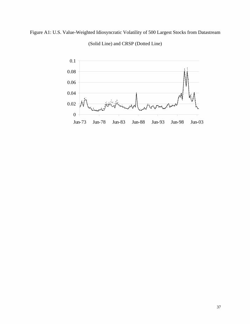
37

Figure A1: U.S. Value-Weighted Idiosyncratic Volatility of 500 Largest Stocks from Datastream

(Solid Line) and CRSP (Dotted Line)

0

0.02

0.04

0.06

0.08

0.1

Jun-73 Jun-78 Jun-83 Jun-88 Jun-93 Jun-98 Jun-03

38

References

Agarwal, D., S. Bharath, and S. Viswanathan, 2004, Technological Change and Stock Return

Volatility: Evidence from eCommerce Adoptions, Unpublished Working paper, University of

Michigan.

Ang, A., R. Hodrick, Y. Xing, and X. Zhang, 2006a, the Cross-Section of Volatility and

Expected Returns, Journal of Finance, 51, 259-299.

Ang, A., R. Hodrick, Y. Xing, and X. Zhang, 2006b, High Idiosyncratic Volatility and Low

Returns: International and Further U.S. Evidence, Unpublished Working Paper, Columbia

University.

Andersen, T., T. Bollerslev, F. Diebold, and P. Labys, 2003, Modeling and Forecasting Realized

Volatility, Econometrica, 71, 579-625.

Bai, J. and S. Ng, 2002, Determining the Number of Factors in Approximate Factor Models,

Econometrica, 70, 191-221.

Bali, T., N. Cakici, X. Yan, and Z. Zhang, 2005, Does Idiosyncratic Risk Really Matter? Journal

of Finance, 60, 905-929.

Belsley, D., E. Kuh, and R. Welsch, 1980, Regression Diagnostics: Identifying Influential Data

and Sources of Collinearity, John Wiley and Sons, New York, NY.

Berk, J., R. Green, and V. Naik, 1999, Optimal Investment, Growth Options and Security

Returns, Journal of Finance, 54 1153-1607.

Berk, J., R. Green, and V. Naik, 2004, Valuation and Return Dynamics of New Ventures,

Review of Financial Studies, 17, 1-35.

Brennan, M., A. Wang, and Y. Xia, 2004, Estimation and Test of a Simple Model of

Intertemporal Asset Pricing, Journal of Finance, 59, 1743-1775.

39

Campbell, J., 1993, Intertemporal Asset Pricing Without Consumption Data, American

Economic Review, 83, 487-512.

Campbell, J., M. Lettau, B. Malkiel, and Y. Xu, 2001, Have Individual Stocks Become More

Volatile? An Empirical Exploration of Idiosyncratic Risk, Journal of Finance, 56, 1-43.

Campbell, J. and P. Perron, 1991, Pitfalls and Opportunities: What Macroeconomists Should

Know about Unit Roots, NBER Macroeconomics Annual 6, 141-201.

Campbell, J., T. Vuolteenaho, 2004, Bad Beta, Good Beta, American Economic Review, 94,

1249-1275.

Comin, D. and S. Mulani, 2006, Diverging Trends in Macro and Micro Volatility: Facts, Review

of Economics and Statistics, forthcoming.

Comin, D. and T Philippon, 2005, the Rise in Firm-Level Volatility: Causes and Consequences,

NBER Macroeconomics Annual 2005, 20, NBER, MA, in (eds.) M. Gertler and K. Rogoff.

Duffee, G., 1995, Stock Returns and Volatility: A Firm-Level Analysis, Journal of Financial

Economics 37, 399-420.

Elliott, G., T. Rothenberg, and J. Stock, 1996, Efficient Tests for an Autoregressive Unit Root,


Fama, E. and K. French, 1989, Business Conditions and Expected Returns on Stocks and Bonds,

Journal of Financial Economics, 25, 23-49.

Fama, E., and K. French, 1993, Common Risk Factors in the Returns on Stocks and Bonds,


Fama, E., and K. French, 1996, Multifactor Explanations of Asset Pricing Anomalies, Journal of

Finance, 51, 55-84.

40

Fama E., and K. French, 1998, Value versus Growth: The International Evidence, Journal of

Finance, 53, 1975-1999.

Fama E. and J. MacBeth, 1973, Risk, Return, and Equilibrium: Empirical Tests, Journal of

Political Economy, 81, 607-36.

Frazzini, A. and L. Marsh, 2003, Idiosyncratic Volatility in the US and UK Equity Markets,

Unpublished Working Paper, Yale University.

French, K., W. Schwert, and R. Stambaugh, 1987, Expected Stock Returns and Volatility,


Ghysels, E., P. Santa-Clara, and R. Valkanov, 2005, There Is a Risk-Return Tradeoff After All,


Goyal, A. and I. Welch, 2006, A Comprehensive Look at The Empirical Performance of Equity

Premium Prediction, Review of Financial Studies, forthcoming.

Goyal, A. and P. Santa-Clara, 2003, Idiosyncratic Risk Matters! Journal of Finance, 58, 975-

1007.

Greene, W., 1997, Econometric Analysis, Third Edition, Prentice Hall, Upper Saddle River, NJ.

Guo, H. and R. Savickas, 2006, Idiosyncratic Volatility, Stock Market Volatility, and Expected

Stock Returns, Journal of Business and Economic Statistics, 24, 43-56.

Guo, H., R. Savickas, Z. Wang, and J. Yang, 2005, Is the Value Premium a Proxy for Time-

Varying Investment Opportunities: Some Time Series Evidence, Unpublished Working Paper,

the Federal Reserve Bank of St. Louis.

Hamao, Y., J. Mei, and Y. Xu, 2003, Idiosyncratic Risk and the Creative Destruction in Japan,

NBER Working Paper W9642.

Harvey, Campbell, 1991, The World Price of Covariance Risk, Journal of Finance, 46, 111-157.

41

Hong, H. and J. Stein, 2003, Differences of Opinion, Short-Sales Constraints and Market

Crashes, Review of Financial Studies, 16, 487-525.

Kothari, S. and J. Shanken, 1997, Book-to-Market, Dividend Yield, and Expected Market

Returns: A Time-Series Analysis, Journal of Financial Economics, 44, 169-203.

Lehmann, B., 1990, Residual Risk Revisited, Journal of Econometrics, 45, 71-97.

Lettau, M. and S. Ludvigson, 2001, Resurrecting the (C)CAPM: A Cross-Sectional Test When

Risk Premia Are Time-Varying, Journal of Political Economy, 109, 1238-1287.

Lettau, M. and J. Wachter, 2006, Why is Long-horizon Equity Less Risky? A Duration-based

Explanation of the Value Premium, Journal of Finance, forthcoming.

Levy, H., 1978, Equilibrium in an Imperfect Market: A Constraint on the Number of Securities

in the Portfolio, American Economic Review, 68, 643-58.

Malkiel, B. and Y. Xu, 2002, Idiosyncratic Risk and Security Returns, Unpublished Working

Paper, University of Texas at Dallas.

Merton, R., 1973, An Intertemporal Capital Asset Pricing Model, Econometrica, 41, 867-887.

Merton, R., 1980, On Estimating the Expected Return on the Market: An Exploratory

Investigation, Journal of Financial Economics, 8, 323-61.

Mazzucato, M., 2002, The PC industry: New Economy or Early Life-Cycle?, Review of

Economic Dynamics 5, 318–345.

Newey, W. and K. West, 1987, A Simple, Positive Semi-definite, Heteroskedasticity and

Autocorrelation Consistent Covariance Matrix, Econometrica, 55, 703-08.

Ng, S. and P. Perron, 1995, Unit Root Test in ARMA Models with Data Dependent Methods for

the Selection of the Truncation Lag, Journal of American Statistical Association, 90, 268-281.

42

Pastor, L. and P. Veronesi, 2003, Stock Valuation and Learning about Profitability, Journal of

Finance, 58, 1749-1790.

Pastor, L. and P. Veronesi, 2005, Technological Revolutions and Stock Prices, Unpublished

Working Paper, University of Chicago.

Petkova, R., 2006, Do the Fama-French Factors Proxy for Innovations in Predictive Variables?

Journal of Finance, forthcoming.

Pontiff, J. and L. Schall, 1998, Book-to-Market Ratios as Predictors of Market Returns, Journal

of Financial Economics, 49, 141-60.

Schwert, W., 1989, Why Does Stock Market Volatility Change over Time? Journal of Finance,

44, 1115-1153.

Schwert, W., 1990, Stock Volatility and the Crash of ’87, Review of Financial Studies, 3, 77-

102.

Seyhun, N., 1990, Overreaction or Fundamentals: Some Lessons from Insiders’ Response to the

Market Crash of 1987, Journal of Finance, 45, 1363-1388.

Shanken, J., 1992, On the Estimation of Beta-Pricing Models, Review of Financial Studies, 5, 1-

33.

Stambaugh, R., 1999, Predictive Regressions, Journal of Financial Economics, 54, 375-421.

Stivers, C., 2003, Firm-level Return Dispersion and the Future Volatility of Aggregate Stock

Market Returns, Journal of Financial Markets, 6, 389-411.

Vogelsang, T., 1998, Trend Function Hypothesis Testing in the Presence of Serial Correlation,


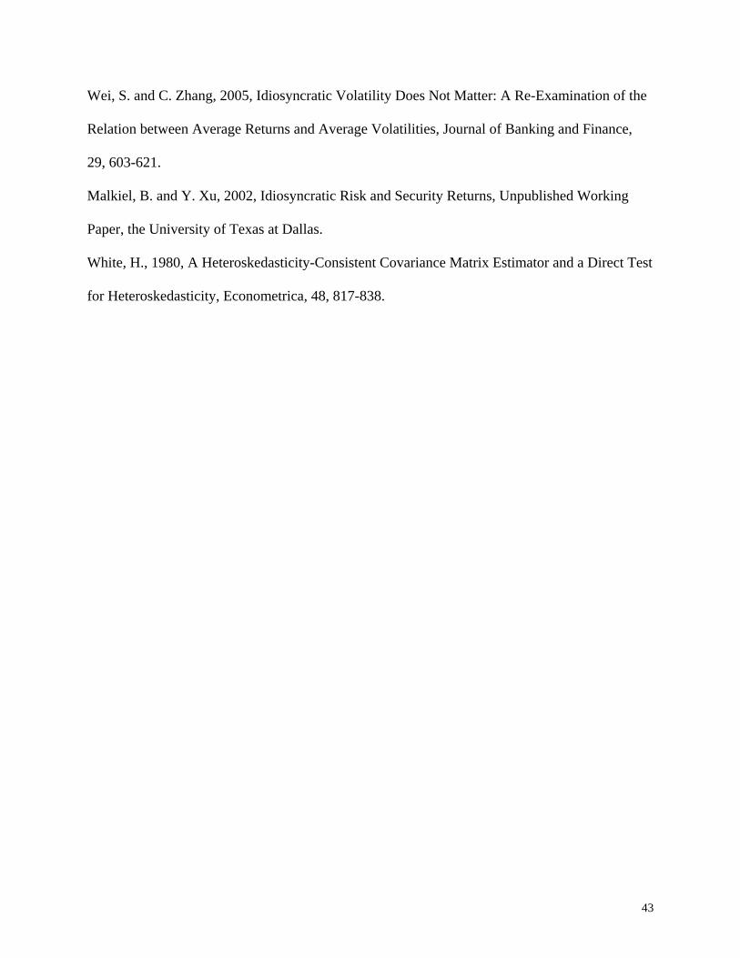
43

Wei, S. and C. Zhang, 2005, Idiosyncratic Volatility Does Not Matter: A Re-Examination of the

Relation between Average Returns and Average Volatilities, Journal of Banking and Finance,

29, 603-621.

Malkiel, B. and Y. Xu, 2002, Idiosyncratic Risk and Security Returns, Unpublished Working

Paper, the University of Texas at Dallas.

White, H., 1980, A Heteroskedasticity-Consistent Covariance Matrix Estimator and a Direct Test

for Heteroskedasticity, Econometrica, 48, 817-838.

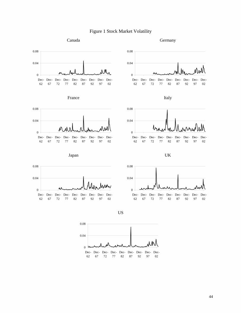
44

Figure 1 Stock Market Volatility

Canada

0

0.04

0.08

Dec-62

Dec-67

Dec-72

Dec-77

Dec-82

Dec-87

Dec-92

Dec-97

Dec-02

Germany

0

0.04

0.08

Dec-62

Dec-67

Dec-72

Dec-77

Dec-82

Dec-87

Dec-92

Dec-97

Dec-02

France

0

0.04

0.08

Dec-62

Dec-67

Dec-72

Dec-77

Dec-82

Dec-87

Dec-92

Dec-97

Dec-02

Italy

0

0.04

0.08

Dec-62

Dec-67

Dec-72

Dec-77

Dec-82

Dec-87

Dec-92

Dec-97

Dec-02

Japan

0

0.04

0.08

Dec-62

Dec-67

Dec-72

Dec-77

Dec-82

Dec-87

Dec-92

Dec-97

Dec-02

UK

0

0.04

0.08

Dec-62

Dec-67

Dec-72

Dec-77

Dec-82

Dec-87

Dec-92

Dec-97

Dec-02

US

0

0.04

0.08

Dec-62

Dec-67

Dec-72

Dec-77

Dec-82

Dec-87

Dec-92

Dec-97

Dec-02

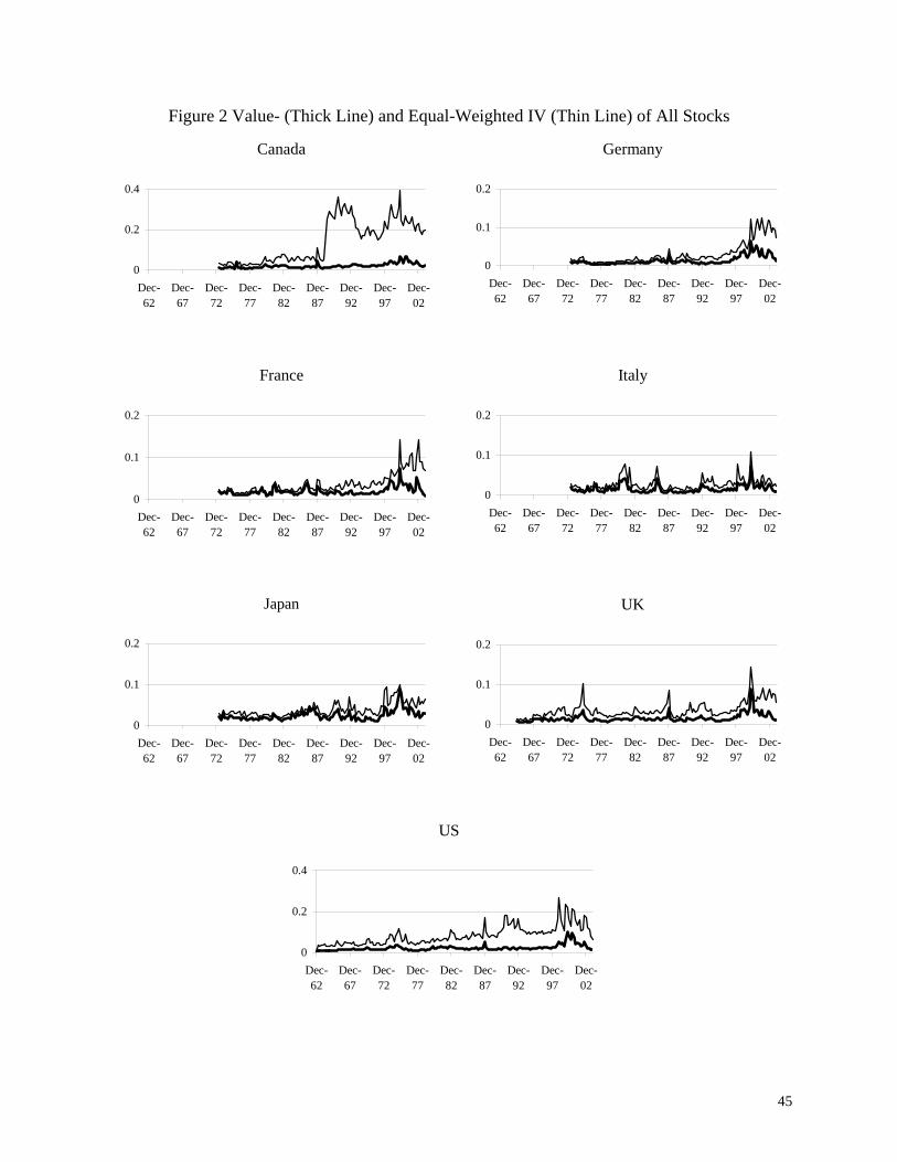
45

Figure 2 Value- (Thick Line) and Equal-Weighted IV (Thin Line) of All Stocks

Canada

0

0.2

0.4

Dec-62

Dec-67

Dec-72

Dec-77

Dec-82

Dec-87

Dec-92

Dec-97

Dec-02

Germany

0

0.1

0.2

Dec-62

Dec-67

Dec-72

Dec-77

Dec-82

Dec-87

Dec-92

Dec-97

Dec-02

France

0

0.1

0.2

Dec-62

Dec-67

Dec-72

Dec-77

Dec-82

Dec-87

Dec-92

Dec-97

Dec-02

Italy

0

0.1

0.2

Dec-62

Dec-67

Dec-72

Dec-77

Dec-82

Dec-87

Dec-92

Dec-97

Dec-02

Japan

0

0.1

0.2

Dec-62

Dec-67

Dec-72

Dec-77

Dec-82

Dec-87

Dec-92

Dec-97

Dec-02

UK

0

0.1

0.2

Dec-62

Dec-67

Dec-72

Dec-77

Dec-82

Dec-87

Dec-92

Dec-97

Dec-02

US

0

0.2

0.4

Dec-62

Dec-67

Dec-72

Dec-77

Dec-82

Dec-87

Dec-92

Dec-97

Dec-02

46

Figure 3 Fitted versus Realized Excess Portfolio Returns

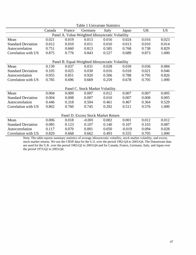
47

Table 1 Univariate Statistics Canada France Germany Italy Japan UK US

Panel A. Value-Weighted Idiosyncratic Volatility Mean 0.021 0.019 0.013 0.016 0.024 0.016 0.023 Standard Deviation 0.012 0.010 0.011 0.010 0.013 0.010 0.014 Autocorrelation 0.751 0.660 0.813 0.585 0.768 0.738 0.829 Correlation with US 0.875 0.776 0.843 0.527 0.689 0.873 1.000

Panel B. Equal-Weighted Idiosyncratic Volatility

Mean 0.139 0.037 0.031 0.028 0.039 0.036 0.084 Standard Deviation 0.105 0.025 0.030 0.016 0.018 0.021 0.046 Autocorrelation 0.955 0.851 0.920 0.506 0.788 0.795 0.826 Correlation with US 0.785 0.696 0.669 0.259 0.678 0.705 1.000

Panel C. Stock Market Volatility

Mean 0.004 0.009 0.007 0.012 0.007 0.007 0.005 Standard Deviation 0.004 0.008 0.007 0.010 0.007 0.008 0.005 Autocorrelation 0.446 0.318 0.504 0.461 0.467 0.364 0.529 Correlation with US 0.802 0.760 0.745 0.292 0.511 0.576 1.000

Panel D. Excess Stock Market Return

Mean 0.006 0.018 -0.001 0.002 0.001 0.012 0.012 Standard Deviation 0.085 0.123 0.107 0.140 0.107 0.103 0.087 Autocorrelation 0.117 0.070 0.001 0.050 -0.019 0.094 0.028 Correlation with US 0.829 0.668 0.662 0.493 0.555 0.705 1.000

Note: The table reports summary statistics of average idiosyncratic volatility, stock market volatility, and excess stock market returns. We use the CRSP data for the U.S. over the period 1962:Q4 to 2003:Q4. The Datastream data are used for the U.K. over the period 1965:Q2 to 2003:Q4 and for Canada, France, Germany, Italy, and Japan over the period 1973:Q2 to 2003:Q4.

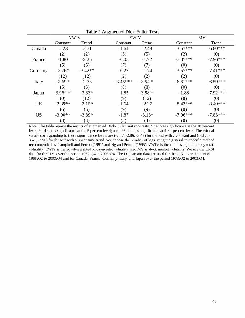
48

Table 2 Augmented Dick-Fuller Tests VWIV EWIV MV Constant Trend Constant Trend Constant Trend

Canada -2.23 (2)

-2.71 (2)

-1.64 (5)

-2.48 (5)

-3.67*** (2)

-6.80*** (0)

France -1.80 (5)

-2.26 (5)

-0.05 (7)

-1.72 (7)

-7.87*** (0)

-7.96*** (0)

Germany -2.76* (12)

-3.42** (12)

-0.27 (2)

-1.74 (2)

-3.57*** (2)

-7.41*** (0)

Italy -2.69* (5)

-2.78 (5)

-3.45*** (8)

-3.54** (8)

-6.61*** (0)

-6.59*** (0)

Japan -3.96*** (0)

-3.33* (12)

-1.85 (9)

-3.58** (12)

-1.88 (8)

-7.92*** (0)

UK -2.89** (6)

-3.15* (6)

-1.64 (9)

-2.27 (9)

-8.43*** (0)

-8.40*** (0)

US -3.00** (3)

-3.39* (3)

-1.87 (3)

-3.13* (4)

-7.06*** (0)

-7.83*** (0)

Note: The table reports the results of augmented Dick-Fuller unit root tests. * denotes significance at the 10 percent level; ** denotes significance at the 5 percent level; and *** denotes significance at the 1 percent level. The critical values corresponding to these significance levels are (-2.57, -2.86, -3.43) for the test with a constant and (-3.12, -3.41, -3.96) for the test with a linear time trend. We choose the number of lags using the general-to-specific method recommended by Campbell and Perron (1991) and Ng and Perron (1995). VWIV is the value-weighted idiosyncratic volatility; EWIV is the equal-weighted idiosyncratic volatility; and MV is stock market volatility. We use the CRSP data for the U.S. over the period 1962:Q4 to 2003:Q4. The Datastream data are used for the U.K. over the period 1965:Q2 to 2003:Q4 and for Canada, France, Germany, Italy, and Japan over the period 1973:Q2 to 2003:Q4.

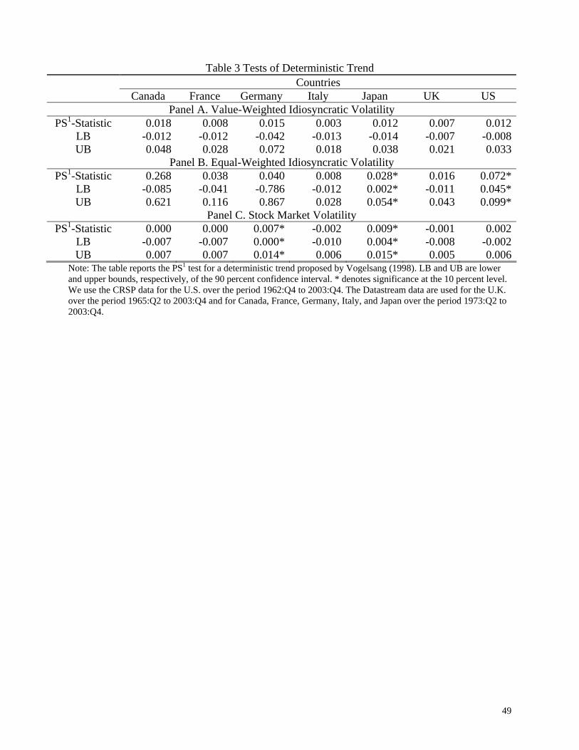
49

Table 3 Tests of Deterministic Trend Countries Canada France Germany Italy Japan UK US

Panel A. Value-Weighted Idiosyncratic Volatility PS1-Statistic 0.018 0.008 0.015 0.003 0.012 0.007 0.012

LB -0.012 -0.012 -0.042 -0.013 -0.014 -0.007 -0.008UB 0.048 0.028 0.072 0.018 0.038 0.021 0.033

Panel B. Equal-Weighted Idiosyncratic Volatility PS1-Statistic 0.268 0.038 0.040 0.008 0.028* 0.016 0.072*

LB -0.085 -0.041 -0.786 -0.012 0.002* -0.011 0.045*UB 0.621 0.116 0.867 0.028 0.054* 0.043 0.099*

Panel C. Stock Market Volatility PS1-Statistic 0.000 0.000 0.007* -0.002 0.009* -0.001 0.002

LB -0.007 -0.007 0.000* -0.010 0.004* -0.008 -0.002UB 0.007 0.007 0.014* 0.006 0.015* 0.005 0.006

Note: The table reports the PS1 test for a deterministic trend proposed by Vogelsang (1998). LB and UB are lower and upper bounds, respectively, of the 90 percent confidence interval. * denotes significance at the 10 percent level. We use the CRSP data for the U.S. over the period 1962:Q4 to 2003:Q4. The Datastream data are used for the U.K. over the period 1965:Q2 to 2003:Q4 and for Canada, France, Germany, Italy, and Japan over the period 1973:Q2 to 2003:Q4.

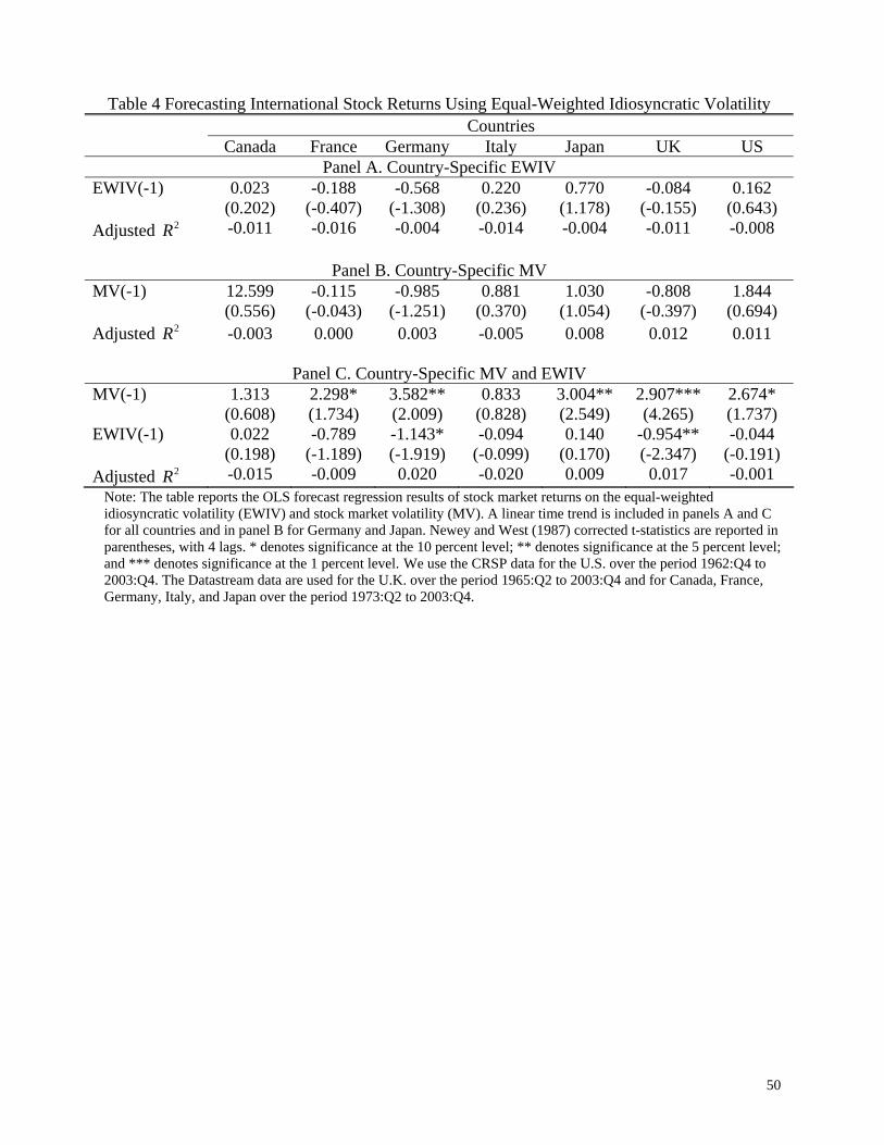
50

Table 4 Forecasting International Stock Returns Using Equal-Weighted Idiosyncratic Volatility Countries Canada France Germany Italy Japan UK US

Panel A. Country-Specific EWIV EWIV(-1) 0.023 -0.188 -0.568 0.220 0.770 -0.084 0.162 (0.202) (-0.407) (-1.308) (0.236) (1.178) (-0.155) (0.643) Adjusted 2R -0.011 -0.016 -0.004 -0.014 -0.004 -0.011 -0.008

Panel B. Country-Specific MV

MV(-1) 12.599 -0.115 -0.985 0.881 1.030 -0.808 1.844 (0.556) (-0.043) (-1.251) (0.370) (1.054) (-0.397) (0.694) Adjusted 2R -0.003 0.000 0.003 -0.005 0.008 0.012 0.011

Panel C. Country-Specific MV and EWIV

MV(-1) 1.313 2.298* 3.582** 0.833 3.004** 2.907*** 2.674* (0.608) (1.734) (2.009) (0.828) (2.549) (4.265) (1.737) EWIV(-1) 0.022 -0.789 -1.143* -0.094 0.140 -0.954** -0.044 (0.198) (-1.189) (-1.919) (-0.099) (0.170) (-2.347) (-0.191) Adjusted 2R -0.015 -0.009 0.020 -0.020 0.009 0.017 -0.001

Note: The table reports the OLS forecast regression results of stock market returns on the equal-weighted idiosyncratic volatility (EWIV) and stock market volatility (MV). A linear time trend is included in panels A and C for all countries and in panel B for Germany and Japan. Newey and West (1987) corrected t-statistics are reported in parentheses, with 4 lags. * denotes significance at the 10 percent level; ** denotes significance at the 5 percent level; and *** denotes significance at the 1 percent level. We use the CRSP data for the U.S. over the period 1962:Q4 to 2003:Q4. The Datastream data are used for the U.K. over the period 1965:Q2 to 2003:Q4 and for Canada, France, Germany, Italy, and Japan over the period 1973:Q2 to 2003:Q4.

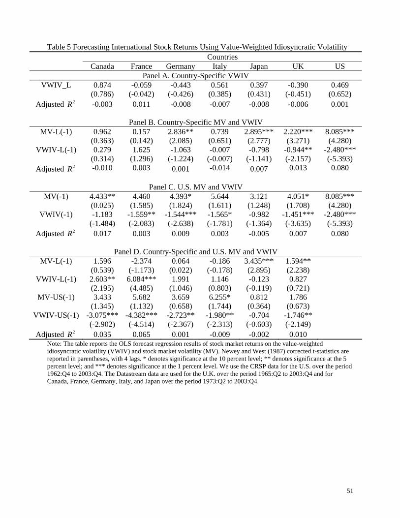
51

Table 5 Forecasting International Stock Returns Using Value-Weighted Idiosyncratic Volatility Countries Canada France Germany Italy Japan UK US

Panel A. Country-Specific VWIV VWIV_L 0.874 -0.059 -0.443 0.561 0.397 -0.390 0.469

(0.786) (-0.042) (-0.426) (0.385) (0.431) (-0.451) (0.652) Adjusted 2R -0.003 0.011 -0.008 -0.007 -0.008 -0.006 0.001

Panel B. Country-Specific MV and VWIV

MV-L(-1) 0.962 0.157 2.836** 0.739 2.895*** 2.220*** 8.085*** (0.363) (0.142) (2.085) (0.651) (2.777) (3.271) (4.280)

VWIV-L(-1) 0.279 1.625 -1.063 -0.007 -0.798 -0.944** -2.480*** (0.314) (1.296) (-1.224) (-0.007) (-1.141) (-2.157) (-5.393)

Adjusted 2R -0.010 0.003 0.001 -0.014 0.007 0.013 0.080

Panel C. U.S. MV and VWIV MV(-1) 4.433** 4.460 4.393* 5.644 3.121 4.051* 8.085***

(0.025) (1.585) (1.824) (1.611) (1.248) (1.708) (4.280) VWIV(-1) -1.183 -1.559** -1.544*** -1.565* -0.982 -1.451*** -2.480***

(-1.484) (-2.083) (-2.638) (-1.781) (-1.364) (-3.635) (-5.393) Adjusted 2R 0.017 0.003 0.009 0.003 -0.005 0.007 0.080

Panel D. Country-Specific and U.S. MV and VWIV

MV-L(-1) 1.596 -2.374 0.064 -0.186 3.435*** 1.594** (0.539) (-1.173) (0.022) (-0.178) (2.895) (2.238)

VWIV-L(-1) 2.603** 6.084*** 1.991 1.146 -0.123 0.827 (2.195) (4.485) (1.046) (0.803) (-0.119) (0.721)

MV-US(-1) 3.433 5.682 3.659 6.255* 0.812 1.786 (1.345) (1.132) (0.658) (1.744) (0.364) (0.673)

VWIV-US(-1) -3.075*** -4.382*** -2.723** -1.980** -0.704 -1.746** (-2.902) (-4.514) (-2.367) (-2.313) (-0.603) (-2.149)

Adjusted 2R 0.035 0.065 0.001 -0.009 -0.002 0.010 Note: The table reports the OLS forecast regression results of stock market returns on the value-weighted idiosyncratic volatility (VWIV) and stock market volatility (MV). Newey and West (1987) corrected t-statistics are reported in parentheses, with 4 lags. * denotes significance at the 10 percent level; ** denotes significance at the 5 percent level; and *** denotes significance at the 1 percent level. We use the CRSP data for the U.S. over the period 1962:Q4 to 2003:Q4. The Datastream data are used for the U.K. over the period 1965:Q2 to 2003:Q4 and for Canada, France, Germany, Italy, and Japan over the period 1973:Q2 to 2003:Q4.

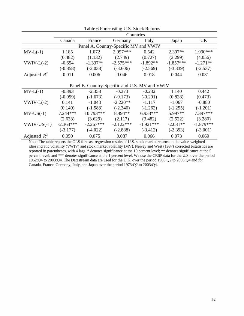
52

Table 6 Forecasting U.S. Stock Returns Countries Canada France Germany Italy Japan UK

Panel A. Country-Specific MV and VWIV MV-L(-1) 1.185 1.072 2.997*** 0.542 2.397** 1.990*** (0.482) (1.132) (2.749) (0.727) (2.299) (4.056) VWIV-L(-2) -0.654 -1.337** -2.575*** -1.892** -1.857*** -1.271** (-0.858) (-2.038) (-3.606) (-2.569) (-3.339) (-2.537) Adjusted 2R -0.011 0.006 0.046 0.018 0.044 0.031

Panel B. Country-Specific and U.S. MV and VWIV

MV-L(-1) -0.393 -2.358 -0.373 -0.232 1.140 0.442 (-0.099) (-1.673) (-0.173) (-0.291) (0.828) (0.473) VWIV-L(-2) 0.141 -1.043 -2.220** -1.117 -1.067 -0.880 (0.149) (-1.583) (-2.340) (-1.262) (-1.255) (-1.201) MV-US(-1) 7.244*** 10.793*** 8.494** 6.933*** 5.997** 7.397*** (2.633) (3.629) (2.117) (3.482) (2.522) (3.280) VWIV-US(-1) -2.364*** -2.267*** -2.122*** -1.921*** -2.031** -1.879*** (-3.177) (-4.022) (-2.888) (-3.412) (-2.393) (-3.001) Adjusted 2R 0.050 0.075 0.087 0.066 0.073 0.069

Note: The table reports the OLS forecast regression results of U.S. stock market returns on the value-weighted idiosyncratic volatility (VWIV) and stock market volatility (MV). Newey and West (1987) corrected t-statistics are reported in parentheses, with 4 lags. * denotes significance at the 10 percent level; ** denotes significance at the 5 percent level; and *** denotes significance at the 1 percent level. We use the CRSP data for the U.S. over the period 1962:Q4 to 2003:Q4. The Datastream data are used for the U.K. over the period 1965:Q2 to 2003:Q4 and for Canada, France, Germany, Italy, and Japan over the period 1973:Q2 to 2003:Q4.

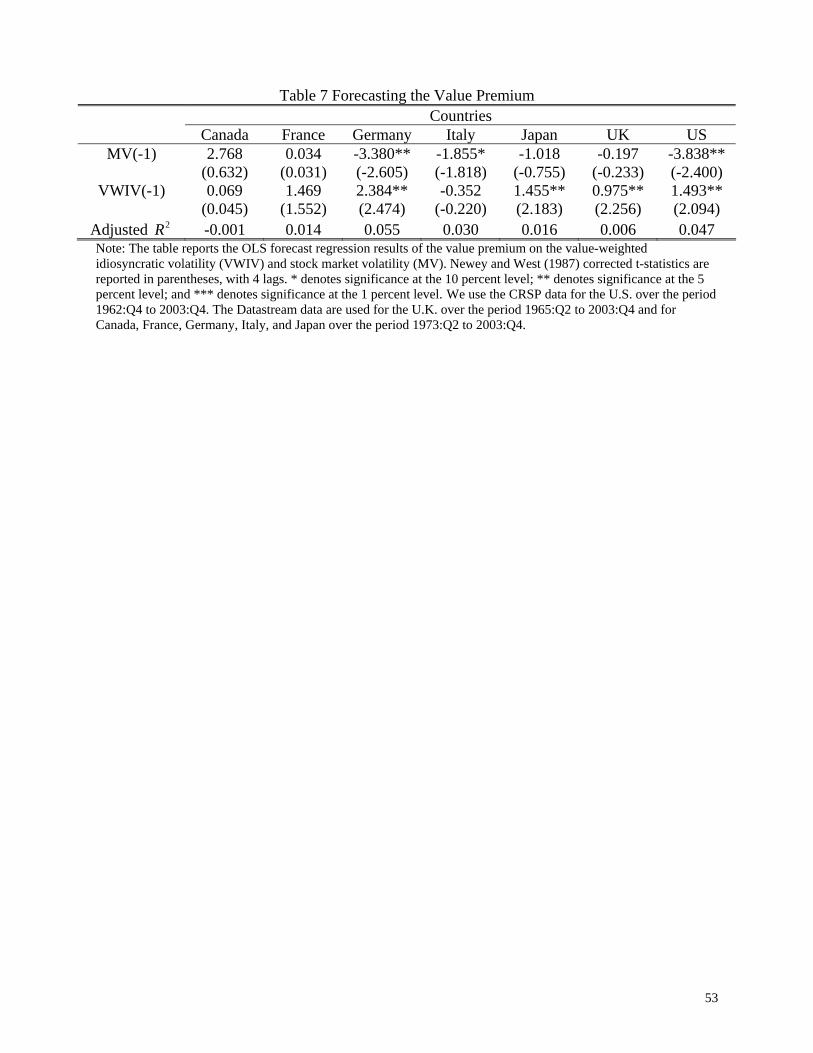
53

Table 7 Forecasting the Value Premium Countries Canada France Germany Italy Japan UK US

MV(-1) 2.768 0.034 -3.380** -1.855* -1.018 -0.197 -3.838** (0.632) (0.031) (-2.605) (-1.818) (-0.755) (-0.233) (-2.400)

VWIV(-1) 0.069 1.469 2.384** -0.352 1.455** 0.975** 1.493** (0.045) (1.552) (2.474) (-0.220) (2.183) (2.256) (2.094)

Adjusted 2R -0.001 0.014 0.055 0.030 0.016 0.006 0.047 Note: The table reports the OLS forecast regression results of the value premium on the value-weighted idiosyncratic volatility (VWIV) and stock market volatility (MV). Newey and West (1987) corrected t-statistics are reported in parentheses, with 4 lags. * denotes significance at the 10 percent level; ** denotes significance at the 5 percent level; and *** denotes significance at the 1 percent level. We use the CRSP data for the U.S. over the period 1962:Q4 to 2003:Q4. The Datastream data are used for the U.K. over the period 1965:Q2 to 2003:Q4 and for Canada, France, Germany, Italy, and Japan over the period 1973:Q2 to 2003:Q4.

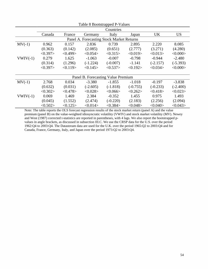
54

Table 8 Bootstrapped P-Values Countries Canada France Germany Italy Japan UK US

Panel A. Forecasting Stock Market Returns MV(-1) 0.962 0.157 2.836 0.739 2.895 2.220 8.085 (0.363)

<0.397> (0.142) <0.499>

(2.085) <0.054>

(0.651) <0.315>

(2.777) <0.019>

(3.271) <0.013>

(4.280) <0.000>

VWIV(-1) 0.279 1.625 -1.063 -0.007 -0.798 -0.944 -2.480 (0.314)

<0.397> (1.296) <0.119>

(-1.224) <0.145>

(-0.007) <0.537>

-1.141 <0.192>

(-2.157) <0.034>

(-5.393) <0.000>

Panel B. Forecasting Value Premium

MV(-1) 2.768 0.034 -3.380 -1.855 -1.018 -0.197 -3.838 (0.632)

<0.302> (0.031) <0.478>

(-2.605) <0.028>

(-1.818) <0.066>

(-0.755) <0.262>

(-0.233) <0.418>

(-2.400) <0.023>

VWIV(-1) 0.069 1.469 2.384 -0.352 1.455 0.975 1.493 (0.045)

<0.502> (1.552) <0.125>

(2.474) <0.014>

(-0.220) <0.384>

(2.183) <0.048>

(2.256) <0.040>

(2.094) <0.043>

Note: The table reports the OLS forecast regression results of the stock market return (panel A) and the value premium (panel B) on the value-weighted idiosyncratic volatility (VWIV) and stock market volatility (MV). Newey and West (1987) corrected t-statistics are reported in parentheses, with 4 lags. We also report the bootstrapped p-values in angle brackets, as discussed in subsection III.C. We use the CRSP data for the U.S. over the period 1962:Q4 to 2003:Q4. The Datastream data are used for the U.K. over the period 1965:Q2 to 2003:Q4 and for Canada, France, Germany, Italy, and Japan over the period 1973:Q2 to 2003:Q4.

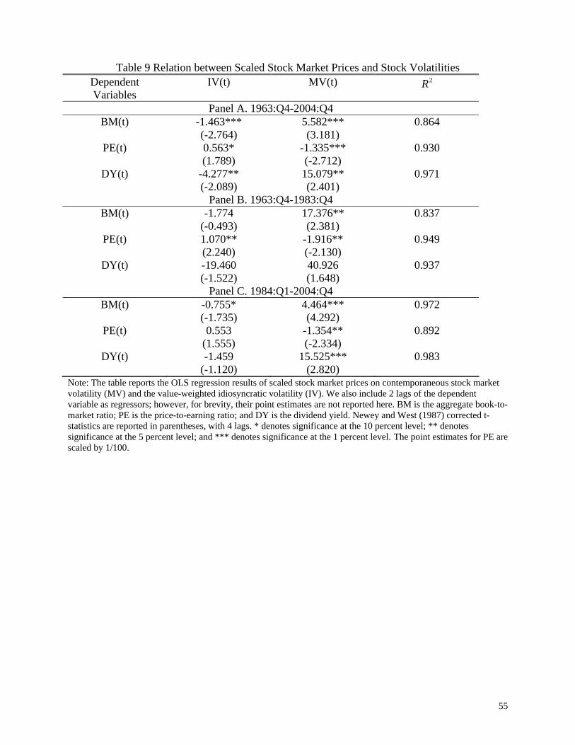
55

Table 9 Relation between Scaled Stock Market Prices and Stock Volatilities Dependent Variables

IV(t) MV(t) 2R

Panel A. 1963:Q4-2004:Q4 BM(t) -1.463***

(-2.764) 5.582*** (3.181)

0.864

PE(t) 0.563* (1.789)

-1.335*** (-2.712)

0.930

DY(t) -4.277** (-2.089)

15.079** (2.401)

0.971

Panel B. 1963:Q4-1983:Q4 BM(t) -1.774

(-0.493) 17.376** (2.381)

0.837

PE(t) 1.070** (2.240)

-1.916** (-2.130)

0.949

DY(t) -19.460 (-1.522)

40.926 (1.648)

0.937

Panel C. 1984:Q1-2004:Q4 BM(t) -0.755*

(-1.735) 4.464*** (4.292)

0.972

PE(t) 0.553 (1.555)

-1.354** (-2.334)

0.892

DY(t) -1.459 (-1.120)

15.525*** (2.820)

0.983

Note: The table reports the OLS regression results of scaled stock market prices on contemporaneous stock market volatility (MV) and the value-weighted idiosyncratic volatility (IV). We also include 2 lags of the dependent variable as regressors; however, for brevity, their point estimates are not reported here. BM is the aggregate book-to-market ratio; PE is the price-to-earning ratio; and DY is the dividend yield. Newey and West (1987) corrected t-statistics are reported in parentheses, with 4 lags. * denotes significance at the 10 percent level; ** denotes significance at the 5 percent level; and *** denotes significance at the 1 percent level. The point estimates for PE are scaled by 1/100.

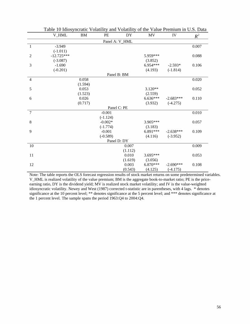
56

Table 10 Idiosyncratic Volatility and Volatility of the Value Premium in U.S. Data V_HML BM PE DY MV IV 2R

Panel A: V_HML 1 -3.949

(-1.011) 0.007

2 -12.725*** (-3.087)

5.959*** (3.852)

0.088

3 -1.690 (-0.201)

6.954*** (4.193)

-2.593* (-1.814)

0.106

Panel B: BM 4 0.058

(1.594) 0.020

5 0.053 (1.523)

3.120** (2.559)

0.052

6 0.026 (0.717)

6.636*** (3.932)

-2.683*** (-4.275)

0.110

Panel C: PE 7 -0.001

(-1.124) 0.010

8 -0.002* (-1.774)

3.905*** (3.183)

0.057

9 -0.001 (-0.589)

6.891*** (4.116)

-2.638*** (-3.952)

0.109

Panel D: DY 10 0.007

(1.112) 0.009

11 0.010 (1.619)

3.695*** (3.056)

0.053

12 0.003 (0.543)

6.870*** (4.125)

-2.690*** (-4.175)

0.108

Note: The table reports the OLS forecast regression results of stock market returns on some predetermined variables. V_HML is realized volatility of the value premium; BM is the aggregate book-to-market ratio; PE is the price-earning ratio, DY is the dividend yield; MV is realized stock market volatility; and IV is the value-weighted idiosyncratic volatility. Newey and West (1987) corrected t-statistic are in parentheses, with 4 lags. * denotes significance at the 10 percent level; ** denotes significance at the 5 percent level; and *** denotes significance at the 1 percent level. The sample spans the period 1963:Q4 to 2004:Q4.

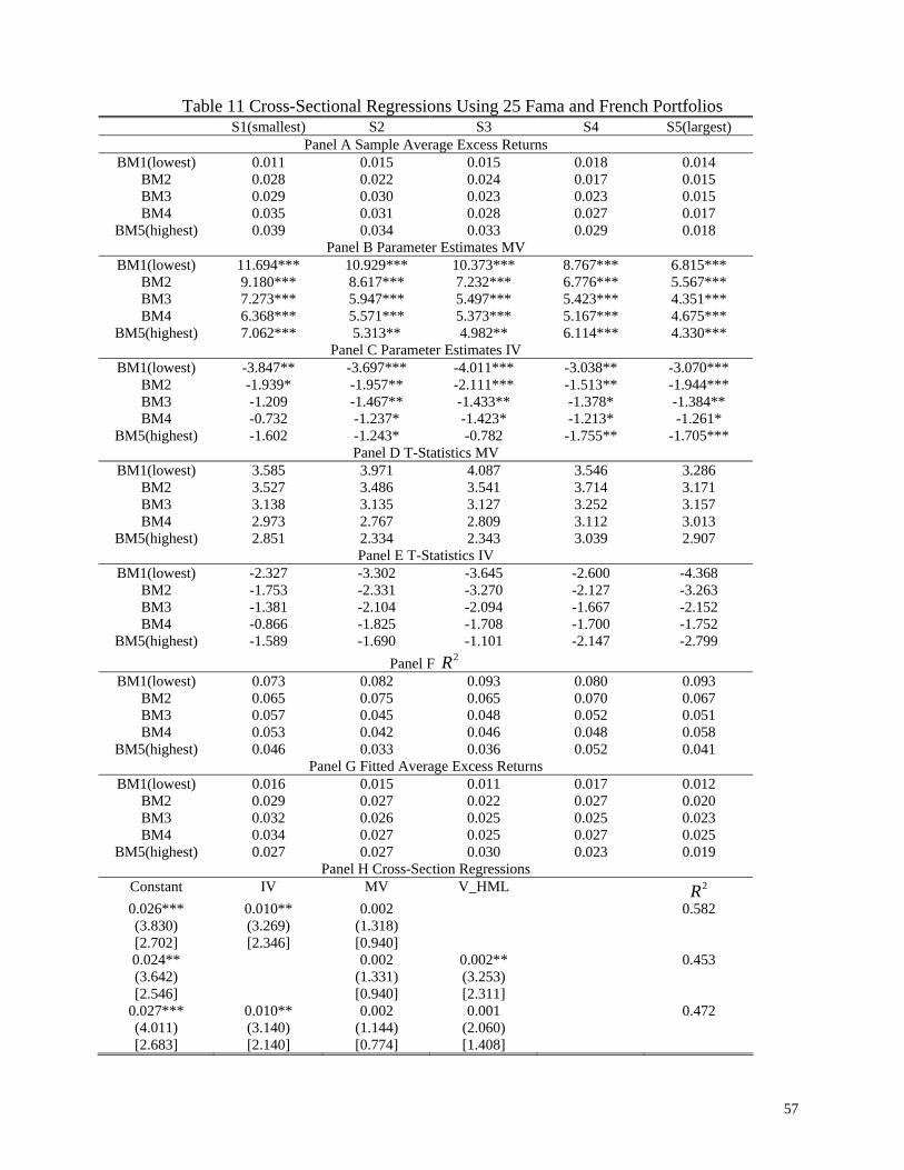
57

Table 11 Cross-Sectional Regressions Using 25 Fama and French Portfolios S1(smallest) S2 S3 S4 S5(largest)

Panel A Sample Average Excess Returns BM1(lowest) 0.011 0.015 0.015 0.018 0.014

BM2 0.028 0.022 0.024 0.017 0.015 BM3 0.029 0.030 0.023 0.023 0.015 BM4 0.035 0.031 0.028 0.027 0.017

BM5(highest) 0.039 0.034 0.033 0.029 0.018 Panel B Parameter Estimates MV

BM1(lowest) 11.694*** 10.929*** 10.373*** 8.767*** 6.815*** BM2 9.180*** 8.617*** 7.232*** 6.776*** 5.567*** BM3 7.273*** 5.947*** 5.497*** 5.423*** 4.351*** BM4 6.368*** 5.571*** 5.373*** 5.167*** 4.675***

BM5(highest) 7.062*** 5.313** 4.982** 6.114*** 4.330*** Panel C Parameter Estimates IV

BM1(lowest) -3.847** -3.697*** -4.011*** -3.038** -3.070*** BM2 -1.939* -1.957** -2.111*** -1.513** -1.944*** BM3 -1.209 -1.467** -1.433** -1.378* -1.384** BM4 -0.732 -1.237* -1.423* -1.213* -1.261*

BM5(highest) -1.602 -1.243* -0.782 -1.755** -1.705*** Panel D T-Statistics MV

BM1(lowest) 3.585 3.971 4.087 3.546 3.286 BM2 3.527 3.486 3.541 3.714 3.171 BM3 3.138 3.135 3.127 3.252 3.157 BM4 2.973 2.767 2.809 3.112 3.013

BM5(highest) 2.851 2.334 2.343 3.039 2.907 Panel E T-Statistics IV

BM1(lowest) -2.327 -3.302 -3.645 -2.600 -4.368 BM2 -1.753 -2.331 -3.270 -2.127 -3.263 BM3 -1.381 -2.104 -2.094 -1.667 -2.152 BM4 -0.866 -1.825 -1.708 -1.700 -1.752

BM5(highest) -1.589 -1.690 -1.101 -2.147 -2.799 Panel F 2R

BM1(lowest) 0.073 0.082 0.093 0.080 0.093 BM2 0.065 0.075 0.065 0.070 0.067 BM3 0.057 0.045 0.048 0.052 0.051 BM4 0.053 0.042 0.046 0.048 0.058

BM5(highest) 0.046 0.033 0.036 0.052 0.041 Panel G Fitted Average Excess Returns

BM1(lowest) 0.016 0.015 0.011 0.017 0.012 BM2 0.029 0.027 0.022 0.027 0.020 BM3 0.032 0.026 0.025 0.025 0.023 BM4 0.034 0.027 0.025 0.027 0.025

BM5(highest) 0.027 0.027 0.030 0.023 0.019 Panel H Cross-Section Regressions

Constant IV MV V_HML 2R 0.026*** (3.830) [2.702]

0.010** (3.269) [2.346]

0.002 (1.318) [0.940]

0.582

0.024** (3.642) [2.546]

0.002 (1.331) [0.940]

0.002** (3.253) [2.311]

0.453

0.027*** (4.011) [2.683]

0.010** (3.140) [2.140]

0.002 (1.144) [0.774]

0.001 (2.060) [1.408]

0.472

58

Note: Panel A reports the sample average of excess returns on 25 Fama and French portfolios. We also run the OLS forecast regression of the portfolio returns on stock market volatility (MV) and the value-weighted idiosyncratic volatility (IV). Panel B reports the point estimates of the coefficient on stock market volatility and panel D reports the corresponding Newey and West (1987) corrected t-statistics; panel C reports the point estimates of the coefficient on the value-weighted idiosyncratic volatility and panel E reports the corresponding Newey and West (1987) corrected t-statistics; and panel F reports the R-squared. In panel H, we report the cross-sectional regression results using the Fama and MacBeth (1973) method. The Fama and MacBeth t-statistics are reported in parentheses and the Shanken (1992) corrected t-statistics are reported in squared brackets. Panel G reports the fitted value using the model with the value-weighted idiosyncratic volatility and stock market volatility as risk factors. * denotes significance at the 10 percent level; ** denotes significance at the 5 percent level; and *** denotes significance at the 1 percent level. The sample spans the period 1963:Q4 to 2004:Q4.

59

Table 12 Cross-Sectional Regressions Using International Data Panel A Forecasting Portfolio Returns

Country Value Stocks Growth Stocks Mean MV T(MV) IV T(IV) 2R Mean MV T(MV) IV T(IV) 2R U.S. 0.027 3.566*** 2.689 -0.615 -0.991 0.049 0.022 6.297** 2.555 -2.465*** -4.119 0.084 Japan 0.029 4.215 1.629 -1.259 -1.226 0.020 0.005 4.285* 1.816 -2.938*** -2.680 0.046 U.K. 0.040 4.945 1.348 -1.682** -2.423 0.029 0.026 6.606* 1.814 -3.996*** -5.633 0.091 France 0.040 5.805 1.629 -2.443** -2.087 0.031 0.019 5.660** 2.015 -3.526*** -3.782 0.071 Germany 0.031 2.831 1.333 -2.187** -2.299 0.032 0.012 6.193** 2.249 -3.795*** -3.946 0.092 Italy 0.031 5.140 1.337 -2.913** -2.379 0.028 0.006 7.369** 2.318 -3.888*** -3.439 0.069 Netherlands 0.023 6.528** 2.195 -3.035*** -2.887 0.034 0.024 4.162* 1.849 -2.897*** -4.799 0.069 Belgium 0.043 4.823** 2.437 -1.640** -2.551 0.032 0.026 4.197** 2.146 -2.938*** -3.302 0.063 Switzerland 0.023 3.097 1.566 -3.071*** -4.333 0.055 0.021 1.777 0.681 -1.693** -2.212 0.019 Sweden 0.039 6.259*** 3.016 -2.156** -2.376 0.038 0.027 9.341*** 4.083 -4.992*** -2.968 0.103 Australia 0.040 3.870** 2.492 -1.357 -1.496 0.018 0.010 6.153*** 3.766 -2.616*** -4.072 0.048 Hong Kong 0.051 7.707** 2.106 -2.767*** -3.301 0.035 0.035 5.263 1.542 -2.987*** -3.162 0.026 Singapore 0.033 11.922*** 2.704 -2.890*** -2.630 0.095 0.016 8.015** 2.258 -3.068*** -2.925 0.053 World 0.029 4.949*** 2.727 -1.884*** -3.597 0.051

0.011 5.356*** 2.667 -3.188*** -4.762 0.099 Panel B Cross-Sectional Regressions

Constant MV IV V_HML MKT HML 2R 0.035*** (4.212) [3.592]

0.002 (1.121) [0.968]

0.007** (2.357) [2.045]

0.238

0.035*** (4.284) [3.597]

0.002 (1.210) [1.199]

0.001** (2.339) [1.997]

0.219

0.032*** (3.029) [2.913]

-0.007 (-0.473) [-0.462]

0.014** (2.436) [2.400]

0.238

Note: The value and growth portfolios are constructed according to the cash flows-to-prices ratio. For each country, the value portfolio includes stocks with the ratio in the top 30% and the growth portfolio includes stocks with the ratio in the bottom 30%. All the portfolio returns are denominated in the U.S. dollar. In panel A we use U.S. value-weighted idiosyncratic volatility (IV) and U.S. stock market volatility (MV) to forecast international portfolios returns and report the Newey and West (1987) corrected t-statistics. In panel B, we report the cross-sectional regression results using the Fama and MacBeth (1973) method. The Fama and MacBeth t-statistics are reported in parentheses and the Shanken (1992) corrected t-statistics are reported in squared brackets. V_HML is realized volatility of the U.S. value premium; MKT is the world excess stock market return, and HML is the world value premium. * denotes significance at the 10 percent level; ** denotes significance at the 5 percent level; and *** denotes significance at the 1 percent level. The sample spans the period 1975:Q1 to 2004:Q4.

average idiosyncratic volatility in g7 countries

Documents