Financial Reporting Quality and Idiosyncratic Return Volatility

Shiva Rajgopal Julius A. Roller Professor of Accounting

University of Washington Box 353200

Seattle, WA 98195 Tel: 206 543 7913 Fax: 206 685 9392

E-mail: rajgopal@u.washington.edu

Mohan Venkatachalam* Fuqua School of Business

Duke University P.O. Box 90120

Durham, NC 27708 Tel: 919 660 7859 Fax: 919 660 7971

E-mail: vmohan@duke.edu

February 2010

Abstract: Campbell, Lettau, Malkiel and Xu (2001) document that firms’ stock returns have become more volatile in the U.S. since 1960. We hypothesize and find that deteriorating earnings quality is associated with higher idiosyncratic return volatility over 1962-2001. These results are robust to controlling for (i) inter-temporal changes in the disclosure of value-relevant information, sophistication of investors and the possibility that earnings quality can be informative about future cash flows; (ii) stock return performance, cash flow operating performance, cash flow variability, growth, leverage and firm size; and (iii) new listings, high-technology firms, firm-years with losses, mergers and acquisitions and financial distress.

*Corresponding Author. We acknowledge helpful comments from , Bill Baber, Anne Beatty, Sanjeev Bhojraj, Michael Brandt, Uday Chandra, Dan Collins (referee), Jennifer Francis, Jon Garfinkel, Cam Harvey, Christopher Jones, Irene Kim, Ryan LaFond, Thomas Z. Lys (editor), Mark Nelson, Per Olsson, Darren Roulstone, Terry Shevlin, Siew Hong Teoh and workshop participants at Cornell University, George Washington University, Ohio State University, University of Iowa, University of Kentucky and the 2005 American Accounting Association Conference. We also acknowledge financial support from the University of Washington Business School and Fuqua School of Business, Duke University.

1

Financial Reporting Quality and Idiosyncratic Return Volatility

1. Introduction

Campbell, Lettau, Malkiel and Xu (2001) document an intriguing result – the

level of average stock return volatility has increased considerably from 1962 to 1997 in

the U.S. Furthermore, most of this increase is attributable to idiosyncratic stock return

volatility as opposed to the volatility of the stock market index. In a similar vein, Morck,

Yeung and Yu (2000) find that the ratio of idiosyncratic risk to systematic risk has surged

over time in the U.S. This upward trend in idiosyncratic volatility has important

implications for (i) portfolio diversification; (ii) arbitrageurs, who require substitutes for

mispriced stocks with lower idiosyncratic risk; and (iii) the pricing of employee stock

options and managerial compensation policies.

In this paper, we explore whether deteriorating financial reporting quality, proxied

by accrual-based measures of earnings quality, is associated with increase in idiosyncratic

volatility over the last four decades.1 Kothari (2000) points to rising stock return

volatility around the globe and wonders whether transparency in financial statement

information is related to these trends in stock return volatility. Several practitioner

accounting bodies, most notably ‘the Jenkins Committee,’ contend that the traditional

financial statements have lost their usefulness due to the transition of the U.S. economy

from a manufacturing to a high-technology, intangible and information-intensive service

oriented economy. Our paper provides evidence consistent with this conjecture.

1 There is neither an agreed upon meaning of the terms “financial reporting quality” and “earnings quality” nor a generally accepted approach to measure them. We assume poor earnings quality or poor financial reporting quality to be consistent with financial statements that are not transparent. Pownall and Schipper (1999) define transparency as an accounting or disclosure system that “reveals the events, transactions, judgments and estimates underlying the financial statements and their implications.” Our proxies (Dechow-Dichev earnings quality measure and squared abnormal accruals discussed in more detail in Section 3) are intended to capture the transparency of financial reporting numbers.

2

Recent accounting research that examines the trends in informativeness of

accounting numbers has reported mixed findings. Collins, Maydew and Weiss (1997),

Francis and Schipper (1999) and Landsman and Maydew (2002) use trends in R2 from a

regression of price/returns on accounting variables to conclude that the informativeness

of financial statements has either stayed constant or increased over time. However,

Brown, Lo and Lys (1999) argue that R2 is an unreliable statistic due to scale effects and

correcting for scale alters inferences (see also Lev and Zarowin 1999). In contrast to

these studies, we focus on different market based measures (the variance of stock returns)

and financial reporting quality variables (earnings quality) and find that deterioration in

financial reporting quality is related to rising idiosyncratic volatility over the last 40

years.

We investigate whether the upward trend in idiosyncratic volatility is related to

earnings quality operationalized in two ways: the extent to which accounting accruals

map into operating cash flows as in Dechow and Dichev (2002) (DD), and squared

abnormal accruals (ABACC2). The earnings quality measures we consider are based on

two distinct but related measurement approaches. The first, the DD measure, is based on

Dechow and Dichev (2002) who argue that the better the mapping of accounting accruals

into past, current and future annual operating cash flows, the greater the earnings quality.

DD captures the extent to which accruals do not map into cash flows, hence it represents

an inverse measure of earnings quality. The ABACC2 measure is based on the modified

Jones’ (1991) model of the normal component of accruals. This approach assumes that

accruals are determined by fundamental shifts in operating activities of the firm such as

revenues and fixed assets and any deviations from such fundamentals are due to

3

managerial manipulation. We consider the squared abnormal accruals as an inverse

measure of earnings quality because greater deviations from the accrual determinants

model reflect greater earnings management.2

Using data from 1962 to 2001, we document a noticeable decline in earnings

quality (based on increasing DD and ABACC2) over time. To examine whether financial

reporting quality is related to idiosyncratic return volatility we conduct two sets of

analyses. First, we verify that, in the cross-section, earnings quality explains differences

in firm specific idiosyncratic volatility. Second, and more pertinent, we investigate

whether the time series trend in return volatility is associated with time trends in earnings

quality. We conduct a time-series analysis because identifying a cross-sectional

association between idiosyncratic volatility and financial reporting quality does not

automatically imply a time-series relation between these constructs.

Consistent with theory that worsening earnings quality causes noisier earnings

(e.g., Diamond and Verrecchia 1991; Leuz and Verrecchia 2000; Easley and O’Hara

2004 and O’Hara 2003), results from time-series and cross-sectional regressions indicate

a strong association between rising idiosyncratic return volatility and falling earnings

quality. These results obtain after controlling for several potential confounds. First,

increasing trends in voluntarily disclosure of other value-relevant information, for

example, via conference calls or via the release of pro-forma earnings (see Francis,

Schipper and Vincent 2002, Collins, Li and Xie 2009) could explain trends in

idiosyncratic volatility. Second, an increase in idiosyncratic volatility could reflect

greater trading by unsophisticated traders in the capital market through the advent of

2 We use the squared discretionary accruals because Cohen, Dey and Lys (2008) suggest that this transformation has more desirable distributional properties than the absolute value of abnormal accruals. Results using the absolute value of abnormal accruals are similar.

4

electronic trading. Third, worsening earnings quality over time could potentially be

informative about firms’ deteriorating future cash flows (see Watts and Zimmerman 1986

and Subramanyam 1996). Finally, the relation between earnings quality and

idiosyncratic volatility could merely reflect the effects of other omitted variables such as

stock return performance, operating performance, cash flow variability, book-to-market

ratio, leverage and firm size.

Although we control for a wide variety of potentially omitted firm characteristics,

endogeneity is always a concern in studies such as ours. We attempt to address

endogeneity concerns by conducting a “changes” analysis and we confirm that firms with

the largest decrease (increase) in earnings quality also experience the largest increase

(decrease) in idiosyncratic return volatility. Next, we investigate institutional factors and

trends in financial reporting practices that might contribute to the time-series association

between financial reporting quality and idiosyncratic volatility. We find that the

temporal link between idiosyncratic volatility and the two information quality proxies

persists even after (i) recognizing the spurt in new listings in the 1980s documented by

Fama and French (2004); (ii) controlling for technology-intensive firms where new

business models may decrease the quality of accounting information; (iii) identifying

firm-years with negative earnings as the increasing incidence of negative earnings may

have contributed to the decline in earnings quality over the last several decades (Collins,

Pincus and Xie 1999); (iv) controlling for mergers and acquisitions activity; and (v)

financial distress.

In supplementary analyses, we document that decreases in earnings quality are

associated with higher return volatility via increased dispersion in analysts’ forecasts.

5

The intuition is that if earnings quality falls, we would expect analysts to place less

weight on the common earnings signal and to place greater weight on other – possibly

idiosyncratic – private information about a firm’s future prospects. This, in turn, impacts

return volatility if different investors follow different analysts.

We make two important contributions. First, we document that earnings quality

has systematically fallen over the last 40 years. Although we do not claim that falling

earnings quality and rising idiosyncratic volatility are necessarily causally related to one

another, this temporal association appears, on the surface, to be consistent with

practitioner complaints that financial reports have become more opaque and less relevant

over time. Second, we are among the first to empirically identify the role of deteriorating

earnings quality as an important factor associated with the temporal increase in

idiosyncratic volatility documented by Campbell et al. (2001). In that sense, we integrate

the literature in finance related to time trends in idiosyncratic volatility with the literature

in accounting related to time trends in the informativeness of accounting numbers for

market participants.

The remainder of the paper proceeds as follows. Section 2 discusses related

research and develops the hypothesized relation between financial reporting quality and

idiosyncratic volatility. Section 3 discusses the empirical measures of earnings quality

(DD and ABACC2). Section 4 reports the sample selection process, measurement of key

variables and descriptive statistics. Section 5 features the results of the cross-sectional

and time-series regressions linking idiosyncratic volatility with earnings quality. In

Section 6, we consider the robustness of our findings to several institutional and

6

accounting factors that may explain the time-series trends in idiosyncratic risk and

earnings quality. We present our conclusions in Section 7.

2. Related Research and Hypothesis 2.1 Stock return volatility

Campbell et al. (2001) find that the volatility of the stock market has remained

relatively constant over the period 1962 to 1997. However, idiosyncratic volatility has

increased substantially over this time period to a point where idiosyncratic volatility is

the largest component of firm-specific return volatility. Campbell et al. (2001) suggest a

number of possible explanations for this phenomenon including increasing leverage,

higher incidence of spin-offs of conglomerates, firms issuing stocks earlier in their life-

cycles and increase in option-based compensation. We are aware of three papers that

explore some of these conjectures. Xu and Malkiel (2003) investigate whether shocks to

institutional sentiment explain the idiosyncratic volatility of stock returns. They find that

the proportion of institutional ownership is correlated with volatility. Wei and Zhang

(2006) find that variation in firm performance over time is related to the inter-temporal

variation in idiosyncratic volatility. Irvine and Pontiff (2009) attribute the Wei and

Zhang (2006) result to fundamental cash flow shocks on account of rising economy-wide

competition. Following Kothari (2000) and O’Hara (2003) we identify deteriorating

financial reporting quality as another explanation for the upward trend in idiosyncratic

volatility.3

3 Morck, Yeung and Yu (2000) and Jin and Myers (2006) document a cross-sectional association between lower stock market synchronicity (measured as the R2 of the regression of firm stock returns on the returns to a market index) and higher transparency of financial reporting across countries. This suggests that lower R2 and hence, higher idiosyncratic volatility implies more opaqueness. Several recent papers question whether lower R2 from a market model implies that the information environment is better (e.g., Hou, Peng

7

2.2 Financial reporting quality and idiosyncratic volatility

Improving disclosures and the quality of financial reporting mitigate information

asymmetries about a firm’s performance and reduce the volatility of stock prices

(Diamond and Verrecchia, 1991; Healy, Hutton and Palepu, 1999). An increase in stock

return volatility is likely to increase the information asymmetric component of the cost of

capital (Leuz and Verrecchia 2000; Froot, Perold and Stein 1992).4

In the finance literature, Easley and O’Hara (2004) and O’Hara (2003) posit that a

firm’s accounting treatment of earnings and its disclosure policy — its financial reporting

quality — can influence the firm’s information environment (information risk) and

consequently, its idiosyncratic volatility and the cost of capital. Francis, LaFond, Olsson

and Schipper (2005) and Aboody, Hughes and Liu (2005) use accounting earnings

quality as a proxy for information risk and demonstrate that earnings quality is related to

expected returns. However, neither paper examines the cross-sectional or time-series

relation between the quality of accounting information and idiosyncratic volatility.

Leuz and Verrecchia (2000) examine the consequences of improved disclosure

quality on a firm’s bid-ask spreads, trading volume and stock-return volatility in the

context of German firms that switched from German GAAP to U.S. GAAP or IAS. They

and Xiong 2006, Ashbaugh-Skaife, Gassen, and LaFond 2006, Kelly 2007, Bartram, Brown, and Stulz 2009, Dasgupta, Gan, and Gao 2009; and Teoh, Yang and Zhang 2009). The evidence in our paper that higher idiosyncratic volatility (and hence lower R2 from a market model regression) is positively related to poorer earnings quality is also inconsistent with the findings of Morck et al. (2000) and Jin and Myers (2006). 4 Note that the broader question of whether idiosyncratic volatility is priced by the stock market is controversial. For example, Goyal and Santa-Clara (2003) argue that idiosyncratic volatility is associated with returns to the market index while Bali, Cakici, Yan and Zhang (2005) show that the Goyal and Santa-Clara (2003) result is specific to certain time periods and is attributable only to small stocks. Even if idiosyncratic risk were not priced in stock returns, we believe that documenting a link between deteriorating financial reporting quality and increasing stock return volatility is valuable. This is because increasing stock return volatility has important implications for arbitrage opportunities, portfolio diversification and stock option pricing.

8

hypothesize that German firms switch to an arguably better financial reporting regime,

commit to increased disclosure and hence experience a reduction in the asymmetric

information component of the cost of capital. The authors find that bid-ask spreads

decline and trading volume improves when German firms switch to an international

reporting regime.

Pastor and Veronesi (2003) posit that significant uncertainty about a firm’s

average profitability influences stock return volatility. To the extent that financial

reporting quality is poor, uncertainty about a firm’s future profitability is likely to be

high. Thus, the Pastor and Veronesi (2003) model is also consistent with the hypothesis

that poor information quality is associated with increased idiosyncratic volatility.5

Note that the above-cited papers argue primarily for a positive association

between poor financial reporting quality and idiosyncratic volatility in the cross-section

of firms. Our focus, however, is on the time-series trends in the two constructs. A priori,

it is conceivable that despite the existence of a cross-sectional relation, there may be no

time-series association between idiosyncratic volatility and deteriorating financial

reporting quality. Nevertheless, we test for a cross-sectional association to i) ensure the

existence of a systematic relation between the two variables and ii) guard against the

charge that we have documented an association between two variables that merely

happen to have increasing time trends.

2.3 What factors other than earnings quality can explain higher stock return volatility?

5 Both Pastor and Veronesi (2003) and Wei and Zhang (2006) find that idiosyncratic volatility is related to volatility of accounting return on equity. However, these papers do not distinguish between sources of increased uncertainty about a firm’s profitability, viz., volatility of cash flow stream as opposed to information about future cash flow volatility arising from the quality of accounting information. Our paper identifies earnings quality as an important determinant of idiosyncratic volatility after controlling for a firm’s underlying cash flow volatility or earnings volatility.

9

Our primary premise is that a decline in earnings quality over time is associated

with higher idiosyncratic stock return volatility. Our empirical test of this premise will

involve documenting a positive inter-temporal association between stock return volatility

and poor earnings quality. However, documenting such an association is potentially

insufficient to validate our claim because changes in idiosyncratic volatility can result

from three confounding factors: (i) changes in the firms’ disclosure of value-relevant

information over time; (ii) changes in the sophistication of investors over time; and (iii)

changes in the signaling role of earnings quality for firms’ future cash flows. We

consider each of these explanations in greater detail below.

2.3.1 Changes in earnings related information over time

Francis, Schipper and Vincent (2002) conduct an analysis of disclosures

(summary income statements with separate disclosure of transitory earnings components,

summary balance sheet and cash flow statement information) released as part of the

earnings announcements and find the temporal increase in return volatility surrounding

earnings announcements is positively associated with these concurrent disclosures.

Collins, Li and Xie (2009) report a temporal increase in firms reporting of Street (non-

GAAP) earnings that leave out items such as restructuring charges and asset impairments.

Moreover, Collins et al. (2009) find that Street earnings surprises are significantly

positively associated with trading volume and return volatility around earnings

announcements suggesting a temporal increase in the intensity of the market’s response

to Street earnings. Together, these papers suggest that expanded disclosures could have

contributed to the temporal increase in the return volatility.

10

2.3.2 Changes in the sophistication of investors over time

Harris (2003) argues that “transitory volatility is due to trading activity by

uninformed traders.” Hence, an alternative explanation for increase in idiosyncratic

volatility over time is a rise in the proportion of “noise traders” in the market, especially

after the advent of on-line trading. Moreover, Lee (1992) documents that small traders

(arguably uninformed) tend to be net buyers around earnings related events. Hedge funds

are also alleged to trade on the earnings surprises without regard for the “fundamentals”

of the stock (Graham, Harvey and Rajgopal 2005).

2.3.3 Earnings quality as a signal of future cash flows

Our claim is that an increase in earnings management reduces the precision of the

earnings signal and is thus related to increased idiosyncratic return volatility. However,

one could counter-argue that earnings management, if detectable by investors, could also

provide additional information to investors (see Watts and Zimmerman 1986). For

example, Subramanyam (1996) finds that the discretionary accruals have positive value

implications in that discretionary accruals (i) are positively related to contemporaneous

returns; and (ii) predict future profitability and dividend changes. He concludes that

managerial discretion improves the informativeness of earnings.

2.4 Empirical design to address these confounds

We attempt to account for the three confounding factors enumerated above in our

research design. In particular, we control for inter-temporal variation in earnings and the

expanded dissemination of value-relevant disclosures by introducing an interaction of a

time-trend and (i) the squared analyst forecast revisions during the fiscal year (FREV2A);

and (ii) the squared annual buy and hold return (RET2). We use forecast revisions and

11

stock returns as two measures that are likely to incorporate value relevant information

disseminated during the fiscal year. Because our left hand side variable, idiosyncratic

volatility, does not depend on the sign of the news, conceptually it would be appropriate

to use unsigned forecast revisions and stock returns. To be consistent with the

measurement of idiosyncratic volatility, measured as the variance of stock returns, we use

the squared transformation of forecast revisions and stock returns. We control for the

inter-temporal variation of the sophistication of investors via an interaction between the

time trend and two proxies for investor sophistication: (i) analyst coverage (NANAL);

and (ii) the proportion of stock ownership held by institutional investors (INST).

To account for the possibility that the positive association between idiosyncratic

return volatility and poor earnings quality could be attributable to increased

informativeness of earnings quality for future cash flows, we include an interaction of the

time-trend and the next year’s operating cash flows (CFOt+1) as a proxy for the

information contained in earnings quality about future cash flows. Thus, after controlling

for all the potential confounds discussed above, if we observe a positive association

between rising idiosyncratic return volatility and falling earnings quality, we can make a

stronger claim that the rising idiosyncratic risk over time is more likely attributable to

noisier earnings due to increasing earnings management.

3. Proxies for financial reporting quality

We consider two measures of earnings quality (DD and ABACC2) as proxies for

financial reporting quality. These measures are described in greater detail below.

12

3.1 Earnings quality measure based on Dechow and Dichev (2002)

Our first measure of earnings quality, DD, is based on an approach proposed by

Dechow and Dichev (2002) and Francis et al. (2005). The underlying premise of this

approach is that earnings quality is primarily determined by the quality of accruals

because accounting earnings can be represented as the sum of operating cash flows and

accruals. The intuition is that accounting accruals either anticipate future operating cash

flows, reflect current cash flows or reversals of past cash flows. Measurement error in

determining accruals could potentially distort the ability of accruals to anticipate future

cash flows or to reflect past and current cash flows. Such measurement error could be the

result of unintentional errors arising from business uncertainty and management lapses,

or due to intentional estimation errors arising from managerial incentives to manipulate

earnings.

The principal idea behind Dechow and Dichev (2002) is to determine the extent

of this measurement error in the mapping of accruals and cash flows. The variance of

this measurement error can be viewed as an inverse measure of earnings quality.

Dechow and Dichev (2002) model the relation between accruals and cash flows as

follows (all variables including the intercept are scaled by average assets):

0 1 1 2 3 1it it it it itTCA CFO CFO CFO v (1)

where TCA is total current accruals calculated as CA – CL – Cash + STDEBT, CA

is change in current assets (Compustat # 4), CL is change in current liabilities

(Compustat # 5), Cash is change in cash (Compustat # 1), STDEBT is change in debt

in current liabilities (Compustat # 34). CFO is cash flow from operations computed as

IBEX –TCA+DEPN, where IBEX is net income before extra-ordinary items (Compustat #

13

18), DEPN is depreciation and amortization expense (Compustat # 14). Subscripts i and t

are firm and time subscripts respectively.

Francis et al. (2005) and McNichols (2002) suggest that the earnings quality

measure derived from (1) can be improved by controlling for two important determinants

of accruals, viz., growth in revenues and the level of property, plant and equipment (see

also Jones (1991)). So, we augment equation (1) as follows:

0 1 1 2 3 1 4 5it it it it it it itTCA CFO CFO CFO REV PPE (1a)

where REV is change in revenues (Compustat # 12), PPE is gross value of property,

plant and equipment (Compustat # 7). We estimate equation (1a) for every firm-year in

each of Fama and French’s (1997) 49 industry groups where we can find at least 20 firms

in year t.6

Under equation (1a), higher accrual quality implies that accruals capture most of

the variation in current, past and future cash flows and, as a consequence, the firm-

specific residual, it, from equation (1a) forms the basis of the earnings quality proxy

used in the study. Specifically, the earnings quality (DDit) metric is defined as the

standard deviation of firm i’s residuals, calculated over years t-4 through t i.e., DDit =

(it-4,t). We treat larger standard deviations of residuals as an indication of poor accruals

and earnings quality.

3.2 Squared abnormal accruals (ABACC2)

As an alternative measure of earnings quality, we consider the firm’s squared

abnormal accruals. This measure relies on the idea that changes in a firm’s accruals are

primarily determined by changes in firm fundamentals particularly, changes in revenues

6 Consistent with Francis et al. (2005), we winsorize the extreme values of the distribution of the

dependent and the independent variables to the 1 and 99 percentiles.

14

and changes in property, plant and equipment. If a firm’s accruals deviate significantly

from the level determined by changes in firm fundamentals then such deviations are

deemed abnormal and such abnormal accruals are assumed to reduce the quality of

accruals and earnings.

To determine abnormal accruals, we apply the modified Jones’ (1991) model, and

estimate the following regression for each of Fama and French’s (1997) 49 industry

groups with at least 20 firms in year t (all variables including the intercept are scaled by

average assets).

0 1 2 3( )it it it it it itTA REV AR PPE ROA (2)

where TA = firm i’s total accruals, computed as TCA-DEPN, AR is change in accounts

receivable (Compustat # 2). Research by Kothari, Leone and Wasley (2005) suggest that

adjusting for firm performance is important when determining abnormal levels of

accruals. Therefore, we include return on assets (ROA) as an additional variable in

equation (2). ROA is IBEX divided by average total assets. The other terms have been

defined before.

We treat the residual, ̂it , from equation (2) as abnormal accruals (ABACC) and

use the squared ABACC as our second proxy for earnings quality. We interpret higher

(lower) values of ABACC2 as measures of lower (higher) earnings quality. An advantage

of ABACC2 over DD is that ABACC2 can be computed for annual intervals (and even

shorter intervals such as quarters as discussed in section 5.4) whereas DD can be

computed only over a five-year moving average window.

Dechow, Ge and Schrand (2009) argue that all earnings quality proxies are

affected by i) fundamental earnings process and ii) errors induced by the accounting

15

system that measures earnings. The fundamental earnings process represents expected

cash flows generated by the firm resulting from the firm’s business model choices and

production decisions. We attempt to account for the fundamental earnings process by

estimating the regression equations (1a), (2) for each industry and through the

introduction of several control variables such as the change in cash sales, the level of PPE

and operating performance that are likely correlated with the fundamental earnings

process. More importantly, when we correlate idiosyncratic volatility and earnings

quality, we control for differences in business models and production functions by

including operating cash flows, the volatility of operating cash flows, stock return

performance, size, book-to-market and leverage as additional control variables.

4. Sample, variable measurement and descriptive statistics 4.1 Sample

We use two samples for conducting the data analyses in this paper: (i) the

Dechow-Dichev (DD) sample; and (ii) the abnormal accruals (ABACC2) sample. The

DD sample and the ABACC2 sample spans the time-period 1962-2001 and is created

from the intersection of stock return volatility data from the CRSP database, which

includes firms from NYSE, AMEX and NASDAQ, and accounting data from

COMPUSTAT.7 Analyst forecast revisions and errors are obtained from IBES database.

Eliminating firms with missing data to calculate both stock return volatility and the DD

measure leaves a sample of 95,270 firm-year observations. The ABACC2 sample, due to

7 Our sample period includes the stock market crashes in 1987 and 2000. To ensure that our results are not driven by these events, we removed observations for three years surrounding the crash period. Untabulated results suggest that our reported inferences are robust to this deletion.

16

fewer variable requirements in estimating abnormal accruals, is slightly larger than the

DD sample and consists of 99,643 firm-year observations.8

4.2 Measurement of variables

We compute two measures of stock return volatility: VARraw and VARFFadj.

VARraw refers to the average monthly variance of raw returns for firm i in fiscal year t.

Monthly variance of raw returns is computed as the sample variance of daily raw returns

within a month, multiplied by the number of trading days in the month. VARFFadj refers to

the average monthly variance of excess returns adjusted for Fama French (1993) three

factor expected returns. Specifically, we measure excess returns as the residual from a

regression of a firm’s daily stock returns on SMB, HML and market beta factors. All our

empirical analyses are based on VARFFadj. Inferences remain the same if we use a

volatility measure based on raw returns or market adjusted returns.

In analyzing the relation between idiosyncratic stock return volatility and

reporting quality, we control for several variables that are posited to influence

idiosyncratic return volatility in the cross-section.

Cash flow volatility:

Vuolteenaho (2002) shows that firm level stock returns are a function of both

expected return news and unexpected cash flow news. In other words, idiosyncratic

return volatility is related to the variance of cash flows. Hence, we control for the

conditional variance in cash flow news via the variance of cash flows (VCFO).9 We

measure VCFO for each firm-year as the variance of annual operating cash flows scaled

8 Our inferences are unchanged when we restrict the ABACC2 sample to the same sample size as the DD sample. 9 Our inferences are unaltered if we use the variance of earnings (scaled by assets or book value of equity) instead of variance of cash flows.

17

by total assets over the trailing five year window for that firm. The relation between

VCFO and stock return volatility is expected to be positive.

Operating performance:

Hanlon, Rajgopal and Shevlin (2004) find that operating performance, defined

either as earnings or operating cash flows scaled by total assets, is negatively associated

with stock return volatility in the cross-section. Therefore, we introduce lagged CFO,

computed as cash flows scaled by average total assets, as a control variable.10

Stock return performance:

Duffie (1995), among others, observes that stock return performance is negatively

related to return volatility. We define firm stock returns (RET) as contemporaneous

annual buy-and-hold returns.

Size:

Pastor and Veronesi (2003) show that small firms experience higher return

volatility. Hence, we control for firm size, where SIZE is the natural logarithm of market

capitalization. Market values are determined three months after the end of fiscal year to

ensure that stock prices reflect all available financial accounting information for that

fiscal year.

Book-to-market:

We expect a negative relation between book-to-market and idiosyncratic return

volatility because firms with greater growth opportunities are likely to be experience

greater stock return volatility. We measure book-to-market as the ratio of book value of

10 Our inferences are unchanged if we use accounting return on assets (ROA) or accounting return on equity (ROE) instead. Callen and Segal (2004) extend Voulteenaho’s (2002) variance decomposition framework to document that in addition to cash flow news, accruals explain return volatility. In untabulated results, we control for accrual volatility in all our empirical specifications and find that none of our inferences change.

18

equity, defined as total assets (Compustat # 6) minus total liabilities (Compustat #181),

divided by the market value of equity.11

Leverage:

Levered firms are more likely to experience financial distress suggesting a

positive association between stock-return volatility and financial leverage in the cross-

section. We define financial leverage (LEV) as the ratio of long-term debt (Compustat

#9 + Compustat #34) to book value of total assets (Compustat #6).

4.3 Descriptive statistics Table 1 presents summary information for the key variables used in the study.

Results indicate that the average monthly idiosyncratic volatility based on raw returns is

about 4% whereas the volatility measure based on the Fama French adjusted returns is

about 3.4%. The average firm has a market capitalization of $75 million (untabulated), a

book-to-market ratio of about 0.99, significant operating cash flows as a percentage of

total assets (5%) and financial leverage of 24% of total assets.12

In order to examine time-trends in return volatility and proxies for financial

reporting quality, we divide the entire sample period into ten four-year sub-periods.

Panel A of Table 2 presents average idiosyncratic return volatility and earnings quality

(both DD and ABACC2 measures) across the various sub-periods. Consistent with prior

research, we find that idiosyncratic volatility has grown by a factor of six over the last

four decades, from 0.92% in the 1962-1965 time window to about 6.03% in the 1998-

11 We do not use common equity (COMPUSTAT#60) as our measure of book equity because this data item contains many missing values until 1966 (see Collins, Maydew and Weiss 1997). 12 To control for potential outliers, we winsorize the financial statement variables in the extreme 1% of the respective distributions. We do not winsorize idiosyncratic volatility to stay consistent with Campbell et el. (2001). However, in untabulated analyses, we verified that idiosyncratic volatility, when winsorized at the 1% and 99% levels, yields inferences similar to those tabulated in the paper.

19

2001 window. The DD measure of earnings quality measure has tripled over the last four

decades rising from 2.01 in the 1962-1965 time frame to 5.96 in the 1998-2001 time-

window. The ABACC2 measure of earnings quality has increased from 0.43 in the 1962-

1965 window to 1.07 in the 1998-2001 window. This implies a significant decline in

earnings quality as higher DD and ABACC2 signify poorer earnings quality. However,

relative to the trend in idiosyncratic volatility, the rate of the increase in DD and

ABACC2 is more evenly distributed over time. To provide a visual representation of the

data in Table 2, we present the time-series trends in idiosyncratic volatility, DD and

ABACC2 in Figure 1. The correlation (not tabled) between the two proxies, DD and

ABACC2, is 0.44 over the entire sample period. Although the correlation is high and

expected, it is not high enough to make one of these proxies redundant. Therefore, we

consider both these proxies in our empirical analysis.

5. Empirical tests of the relation between idiosyncratic volatility and financial reporting quality 5.1 Cross-sectional tests

We begin with a set of cross-sectional regressions of idiosyncratic volatility on

the two proxies of reporting quality, DD and ABACC2 after incorporating the control

variables discussed in section 2.4 and 4.2. Although the primary focus of the paper is the

time-series association between idiosyncratic volatility and financial reporting quality, it

is useful and important to demonstrate the existence of a cross-sectional relation between

idiosyncratic return volatility and reporting quality. We estimate the following cross-

sectional regression that relates return volatility with earnings quality after controlling for

20

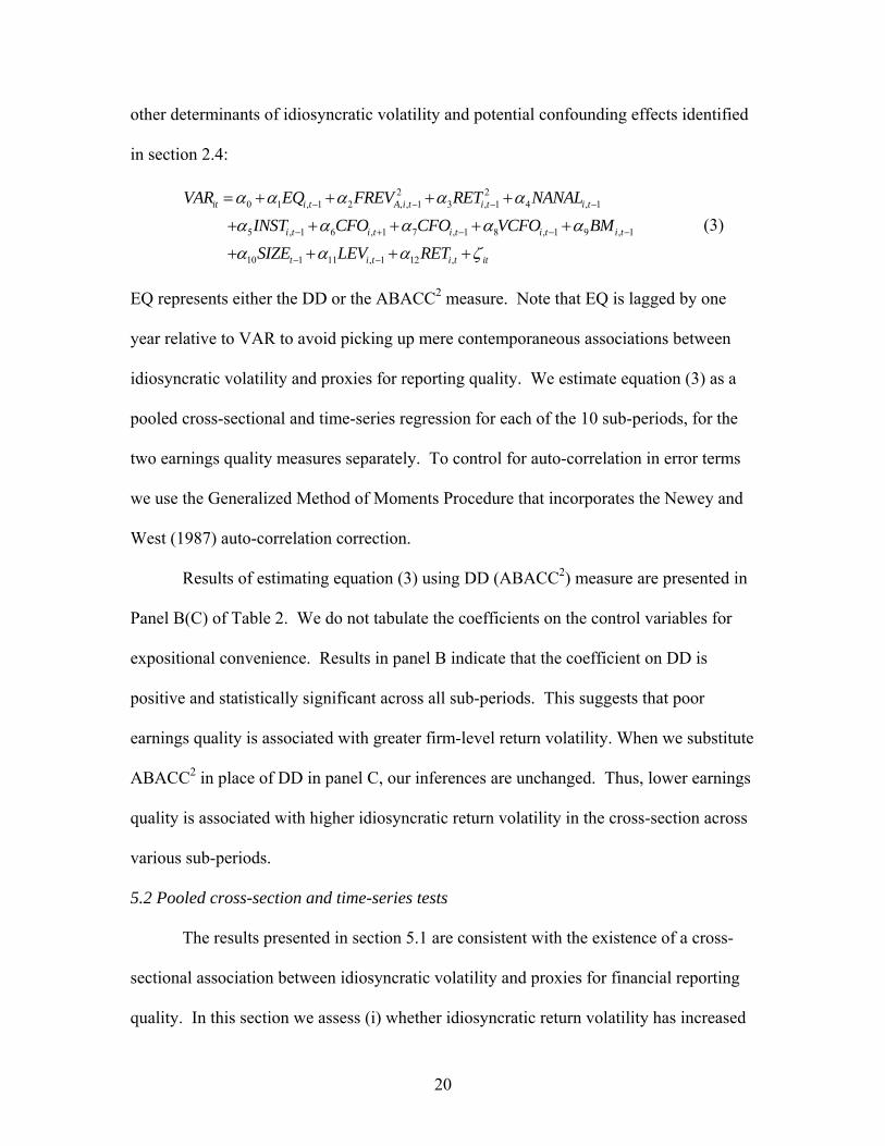
other determinants of idiosyncratic volatility and potential confounding effects identified

in section 2.4:

2 20 1 , 1 2 , , 1 3 , 1 4 , 1

5 , 1 6 , 1 7 , 1 8 , 1 9 , 1

10 1 11 , 1 12 ,

it i t A i t i t i t

i t i t i t i t i t

t i t i t it

VAR EQ FREV RET NANAL

INST CFO CFO VCFO BM

SIZE LEV RET

(3)

EQ represents either the DD or the ABACC2 measure. Note that EQ is lagged by one

year relative to VAR to avoid picking up mere contemporaneous associations between

idiosyncratic volatility and proxies for reporting quality. We estimate equation (3) as a

pooled cross-sectional and time-series regression for each of the 10 sub-periods, for the

two earnings quality measures separately. To control for auto-correlation in error terms

we use the Generalized Method of Moments Procedure that incorporates the Newey and

West (1987) auto-correlation correction.

Results of estimating equation (3) using DD (ABACC2) measure are presented in

Panel B(C) of Table 2. We do not tabulate the coefficients on the control variables for

expositional convenience. Results in panel B indicate that the coefficient on DD is

positive and statistically significant across all sub-periods. This suggests that poor

earnings quality is associated with greater firm-level return volatility. When we substitute

ABACC2 in place of DD in panel C, our inferences are unchanged. Thus, lower earnings

quality is associated with higher idiosyncratic return volatility in the cross-section across

various sub-periods.

5.2 Pooled cross-section and time-series tests

The results presented in section 5.1 are consistent with the existence of a cross-

sectional association between idiosyncratic volatility and proxies for financial reporting

quality. In this section we assess (i) whether idiosyncratic return volatility has increased

21

over time; and (ii) whether such an increase is associated with decreases in reporting

quality. For this analysis, we employ a dataset of pooled cross-sectional and time-series

observations.

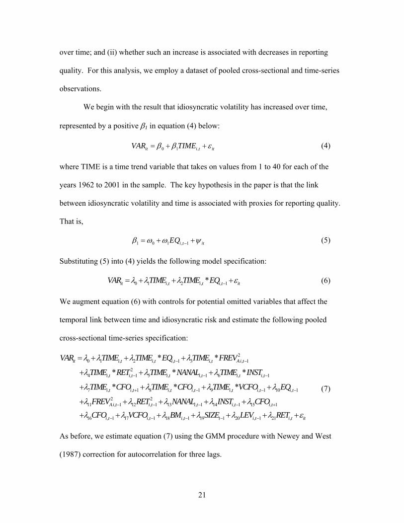
We begin with the result that idiosyncratic volatility has increased over time,

represented by a positive 1 in equation (4) below:

0 1 ,it i t itVAR TIME (4)

where TIME is a time trend variable that takes on values from 1 to 40 for each of the

years 1962 to 2001 in the sample. The key hypothesis in the paper is that the link

between idiosyncratic volatility and time is associated with proxies for reporting quality.

That is,

1 0 1 , 1i t itEQ (5)

Substituting (5) into (4) yields the following model specification:

0 1 , 2 , , 1*it i t i t i t itVAR TIME TIME EQ (6)

We augment equation (6) with controls for potential omitted variables that affect the

temporal link between time and idiosyncratic risk and estimate the following pooled

cross-sectional time-series specification:

20 1 , 2 , , 1 3 , , 1

24 , , 1 5 , , 1 6 , , 1

7 , , 1 8 , , 1 9 , , 1 10 , 1

211 ,

* *

* * *

* * *

it i t i t i t i t Ai t

i t i t i t i t i t i t

i t i t i t i t i t i t i t

Ai

VAR TIME TIME EQ TIME FREV

TIME RET TIME NANAL TIME INST

TIME CFO TIME CFO TIME VCFO EQ

FREV

21 12 , 1 13 , 1 14 , 1 15 , 1

16 , 1 17 , 1 18 , 1 19 1 20 , 1 21 ,

t i t i t i t i t

i t i t i t t i t i t it

RET NANAL INST CFO

CFO VCFO BM SIZE LEV RET

(7)

As before, we estimate equation (7) using the GMM procedure with Newey and West

(1987) correction for autocorrelation for three lags.

22

Consistent with prior research, we predict a positive coefficient on TIME. We

interact time with eight variables in (7): EQ, FREV2A, RET2, NANAL, INST, CFOt+1,

CFOt-1 and VCFO.13 If deterioration in earnings quality explains the increasing trend in

idiosyncratic volatility, we expect a positive coefficient on TIME*EQ after controlling

for the other interaction terms with TIME. As discussed in section 2.4, the interactions of

TIME with FREV2A and RET2 control for the hypothesis that increasing disclosure of

other value-relevant news potentially accounts for the positive coefficient of TIME*EQ.

The interaction terms, TIME*NANAL and TIME*INST, control for changing investor

sophistication over time. We interact TIME with CFOt+1 to address the possibility that

deteriorating earnings quality is potentially informative about future cash flows. The

interactions of TIME with CFOt-1 and VCFO account for the possibility that time-trends

in cash flow performance and variability of cash flows are potential competing

explanations for increases in return volatility. We also include main effects for EQ,

FREV2A, RET2, NANAL, INST, CFOt+1, CFOt-1 and VCFO to control for cross-sectional

differences in these variables during the sample period.14

Table 3 reports the results of estimating equation (7). In discussing our results we

focus on the DD measure (column 1) as the results for the ABACC2 measure (column 2)

are similar. As expected, the coefficient on TIME*DD reported in column (1) is positive

(coefficient = 0.017) and significant (t = 10.51) suggesting that part of the temporal

increase in idiosyncratic volatility is associated with deterioration in earnings quality.

13 For firms and periods prior to 1978 for which analyst forecast revisions are unavailable, we code

forecast revisions as zero. If anything, this treatment would bias against finding a positive coefficient for the variable of interest (TIME*EQ) as the squared FREV would be higher in the post 1978 period than the pre 1978 period.

14 Our inferences are unaffected if we do not include the main effects. Further, in an untabulated sensitivity check, we include TIME interaction terms for SIZE, BM and LEV and find that our inferences are unaltered even after including those additional interaction terms.

23

Consistent with conjectures that increased disclosure of value relevant news is associated

with higher return volatility, we find a positive and significant coefficient on

TIME*RET2 (coefficient = 0.004, t-statistic = 1.62). However, changes in analyst

coverage and institutional owners over time do not appear to be associated with the trend

in idiosyncratic volatility. Consistent with Wei and Zhang (2006) we find that poor

performance is associated with an increase in idiosyncratic risk as the coefficients on

TIME*CFOt-1 and on TIME*CFOt+1 are negative. Note that controlling for the potential

impact of worsening earnings quality on future cash flows via TIME*CFOt+1 does not

affect the positive coefficient on TIME*DD.

5.3 Firm fixed effects analysis

Readers may be concerned that inferences about the association between time-

trends of information quality and return volatility in section 5.2 are based on a pooled-

cross-section and time-series regression where multiple annual observations for the same

firm are used. While the Newey and West (1987) autocorrelation correction mitigates

such concerns, we examine the robustness of our results by estimating a fixed-effects

version of equation (7) where every firm in the sample and every year in the sample is

assigned a dummy variable. Results (unreported) from the fixed-effects model suggest

that the positive coefficients on TIME*DD and TIME*ABACC2 are robust.

5.4 Pure time-series tests

Estimating equation (7) using a pooled cross-sectional time-series dataset, as in

section 5.2, has the advantage of significant statistical power to test our hypothesis that

the secular upward trend in idiosyncratic volatility is related to a similar secular trend in

reporting quality. A potential disadvantage of using a pooled dataset is the possibility of

24

spurious cross-sectional correlations affecting inferences about the time-series relation.

For example, idiosyncratic volatility and proxies for financial reporting quality could be

related in the cross-section without displaying any time-series associations (although

Figure 1 and Table 2 would suggest otherwise). To guard against the possibility that

pooled cross-sectional time-series design potentially induces a spurious significant

coefficient on the TIME*DD (or TIME*ABACC2) while estimating equation (7), we also

conduct a pure time-series test to relate VAR with ABACC2.

A limitation of the time-series test conducted over annual time intervals is the

potential small sample size (n= 40 years) and the consequent low statistical power. To

increase statistical power, we conduct the time-series tests using quarterly time intervals.

We restrict our time-series tests to the ABACC2 earnings quality measure because the

DD measure cannot be easily constructed on a quarterly basis. Because quarterly data for

determining accruals is not available until 1976 from COMPUSTAT and analyst

forecasts are only available for a reasonable sample of firms since 1976 from the Zacks

and IBES databases, we use data available for 104 quarters starting from the first quarter

of 1976 to the fourth quarter of 2001.

In particular, we estimate time-series regressions of the following type:

2 2 20 1 2 1 3 , 1 4 1 5 1 6 1

7 1 8 1 9 1 10 1 11 1 12 1 13

t t t Q t t t t

t t t t t t t t

VAR TIME ABACC FREV RET NANAL INST

CFO CFO VCFO BM SIZE LEV RET

(8)

where VARt is equally-weighted average variance of daily Fama French (1990) three factor

model adjusted returns measured every quarter, and ABACC2t-1 is equally-weighted average

ABACC2 measured every quarter. Abnormal accruals are estimated using the procedure

described in section 3.2 except that we rely on quarterly data. FREVQ is the forecast revision

25

of one quarter ahead earnings as opposed to one year ahead earnings. The other independent

variables in (8) represent equally-weighted quarterly averages.

The regression error-terms from equation (8) are likely to be auto-correlated with

conditional heteroscedasticity. Hence, we employ GMM based t-statistics that use

Newey-West (1987) type corrections (up to three lags) for auto correlation. The

regression results reported in Table 4 support a clear time-series association between

VAR and ABACC2 (coefficient on ABACC2 is 3.399, t-statistic = 1.88). Thus, there is

reliable evidence of a time-series based association between a downward trend in

earnings quality and a concurrent increase in idiosyncratic return volatility.

5.5 Idiosyncratic volatility and analyst forecast dispersion

An alternate test of our premise that worsening earnings quality is associated with

greater idiosyncratic risk is to evaluate how earnings quality affects dispersion of

analysts’ forecasts. Analyst forecasts, like stock prices, are an observable measure of

how investors interpret earnings information. If earnings quality falls, we would expect

analysts to place less weight on the common earnings signal and to place greater weight

on other idiosyncratic private information. This, in turn, may impact return volatility if

different investors follow different analysts. Thus, a decrease in earnings quality is

potentially associated with higher return volatility via increased dispersion in analysts’

forecasts.

One way to empirically evaluate this line of reasoning is to decompose analyst

forecast dispersion (DISP) into the portion explained by falling earnings quality and into

a residual portion. That is, we regress DISP on EQ each year and then obtain the extent of

DISP predicted by EQ (i.e., the predicted value, PDISP) and the error term from such

26

regression (EDISP). Next, we interact TIME with both PDISP and EDISP and insert

these terms in equation (7) instead of TIME*EQ. If the increase in analyst forecast

dispersion is due to analysts increased reliance on idiosyncratic information (perhaps via

diligent acquisition of private information) and lesser reliance on common (noisier)

information, we would expect the coefficient on TIME*PDISP to be greater than the

coefficient on TIME*EDISP. However, we caution the reader that a higher coefficient

on TIME*PDISP relative to TIME*EDISP may obtain due to attenuation bias in

estimating DISP. For example, if EQ is measured with error, it introduces noise in the

estimate of EDISP which in turn causes a downward bias in the coefficient on

TIME*EDISP.

One of the data-related limitations of relying on a dispersion measure is that

analysts are likely to avoid covering small, illiquid firms and hence, the composition of

the sample is unavoidably tilted towards large stocks. We measure forecast dispersion

(DISP) as the ratio of standard deviation of analysts’ earnings forecast to the absolute

value of mean forecast for the fiscal year. In determining DISP we only consider

forecasts issued by analysts during the three months following the month after the end of

the prior fiscal year. This ensures that the earnings forecasts used in determining the

dispersion are made with foreknowledge of the annual earnings of the previous fiscal

year. Also, we consider only the last available forecast for each analyst so as to avoid

duplicate forecasts in constructing the dispersion measure. Because the DISP sample is

drawn from the intersection of the broader sample with that of analyst dispersion data

obtained from Zacks database, the DISP sample is considerably smaller.

27

Results presented in column (1) of Table 5 indicate that TIME*DISP is positively

associated with volatility in a manner similar to the association between TIME*EQ and

volatility. Although this is suggestive of analyst forecast dispersion capturing differences

in earnings quality, it may also reflect differences in private information acquisition.

Results presented in columns (2) and (3) help disentangle the two explanations. The

coefficient on TIME*PDISP is greater than the coefficient on TIME*EDISP in column

(2) where EQ is measured as DD (F-statistic to test the equality of these coefficients =

5.63, p-value = 0.02). In column (4), where EQ is measured as ABACC2, although the

coefficient on TIME*PDISP (0.020) is higher than the coefficient on TIME*EDISP

(0.013) the two coefficients are statistically indistinguishable. Broadly speaking, subject

to the caveats mentioned earlier, the evidence presented here is consistent with our

premise that worsening earnings quality over time is associated with rising idiosyncratic

volatility via increased dispersion in analysts’ forecasts.

5.6 Additional analyses

Our evidence thus far supports an association between increases in stock return

volatility and a concurrent decrease in earnings quality. In this section, we attempt to

provide additional corroborating evidence by examining whether lower earnings quality

is reflected in lower earnings response coefficients and to what extent the relation

between earnings quality and return volatility is concentrated around earnings

announcements.

First, we modify the empirical specification in Ryan and Zarowin (2003) as

follows:

0 1 , 2 , 3 , 1 4 , ,

5 , , , 1

*

* *it i t i t i t i t i t

i t i t i t it

ABRET EARN TIME EQ TIME EARN

TIME EARN EQ

(9)

28

where ABRET is annual abnormal return, measured as fiscal period raw return adjusted

for value weighted market return and EARN is income before extraordinary items for the

year scaled by market value of equity at the beginning of the fiscal year. To be consistent

with previous specifications, we include the main effects as well as the interaction effects

in equation (9).

Table 6, panel A shows that the coefficient on TIME*EARN is negative

suggesting that contemporaneous earnings-returns association has fallen over time

consistent with findings in Ryan and Zarowin (2003). More important, the coefficient on

TIME*EARN*EQ is also negative suggesting that the decline in earnings response

coefficients is associated with a fall in earnings quality (recall that higher EQ reflects

lower earnings quality). Thus, our evidence is consistent with poor accruals quality

leading to a decline in the informativeness of earnings over time.

Next, we examine stock return volatility around earnings announcements because

several papers in the literature starting with Beaver (1968) have investigated this issue.

Note that the preceding analysis documenting a temporal decrease in earnings

informativeness due to poor earnings quality is based on annual returns and not merely on

returns around earnings announcements. Volatility of returns around a small event

window such as earnings announcement window is more likely to capture information as

opposed to noise. Consistent with this notion, Landsman and Maydew (2002) document

that abnormal return volatility around earnings announcements (measured as the return

volatility surrounding earnings announcement days scaled by volatility around non-

announcement days) has increased over time and they interpret this time trend as

consistent with an increase in the informativeness of quarterly earnings. We extend their

29

work to examine whether trends in earnings quality could plausibly be related to trends in

return volatility around earnings announcement dates. In particular, we estimate the

following empirical specification:

2 20 1 , 2 , , 1 3 , , , 1 4 , , 1

5 , , 1 6 , , 1 7 , , 1 8 , 1

2 29 , 1 10 , , 1 11 , 1 12

* * *

* * *it i t i t i t i t EA i t i t i t

i t i t i t i t i t i t i t

i t EA i t i t

EVAR TIME TIME EQ TIME FREV TIME FERR

TIME NANAL TIME PIN TIME CFO EQ

FERR FREV NANAL P

, 1 13 , 1i t i t itIN CFO

(10)

where EVAR is return volatility surrounding earnings announcement days scaled by

average monthly return volatility during the year. Specifically, we compute the variance

of Fama French (1993) three factor model adjusted returns for the seven days

surrounding an earnings announcement and average this variance across all the earnings

announcements for a firm-year. We then scale this by the average monthly variance of

Fama French excess returns for the firm-year. In computing the average monthly

variance we exclude the seven days surrounding earnings announcements.

Recall that declining earnings quality may be associated with rising return

volatility around earnings announcements for other reasons identified in section 2.4: (i)

increased disclosure of other value relevant information; (ii) increased noise trading; and

(iii) earnings quality can potentially be informative about a firm’s future cash flows.

To address these potential confounds, we include several variables. First, we insert an

interaction of TIME and the squared change in the first available consensus analyst

forecast of next quarter’s earnings following the earnings announcement relative to the

last available analyst consensus forecast before the earnings announcement scaled by

stock price at the date of the last available analyst forecast (FREV2EA) as the proxy for

time-based variation in other value-relevant signals about future cash flows released

along with the earnings announcement. Next, we introduce an interaction of TIME and

30

the squared street earnings surprises scaled by stock price (FERR2) to address the concern

that we might be merely picking up what Collins et al. (2009) find. FERR is computed as

the difference between the unadjusted I/B/E/S reported actual earnings per share and the

most recent median consensus earnings forecast immediately prior to the earnings

announcement date scaled by stock price at the date of the last available consensus

forecast. Third, we include interaction terms TIME*INST, TIME *NANAL, and

TIME*PIN to account for changing composition of sophisticated investors over time.

While INST and NANAL capture institutional ownership and analyst following, PIN

refers to the probability of informed trading proposed by Easley et al. (2002).15 The PIN

dataset covers all ordinary common stocks listed on NYSE and AMEX for the years 1983

− 2001. Finally, we introduce an interaction of TIME*CFOt+1 where CFOt+1 is the

quarter-ahead operating cash flows to account for the possibility that earnings quality

potentially inform investors about a firm’s future cash flows. For completeness, we

include the main effects for each of the variables discussed above.

Results of estimating equation (10) are presented in Panel B of Table 6. In

unreported results, absent interaction terms and control variables, we find that the time

trend variable, TIME, is positive and statistically significant suggesting an increase in

earnings announcement window return volatility over time, consistent with Landsman

and Maydew (2002). However, when we introduce the various control variables and

interactive term of time trend variable with earnings quality proxies, TIME, the time

trend variable loses its significance. The coefficient on TIME*INST is positive and

statistically significant suggesting that the increase in return volatility around earnings

15 We obtain PIN scores from Professor Soren Hvidkjaer’s wesbsite (http://www.smith.umd.edu/faculty/hvidkjaer/).

31

announcements is associated with the greater institutional investor holdings over time.

However, the coefficient on the interaction term, TIME*EQ, is positive but not

statistically significant suggesting that the temporal association between annual/quarterly

return volatility and earnings quality documented in sections 5.2, 5.3 and 5.4 is not

concentrated around earnings announcements.16

6. Can institutional and accounting factors explain the time-series relation between idiosyncratic volatility and financial reporting quality?

In this section we examine whether specific institutional and accounting factors

can explain time-trends in both idiosyncratic risk as well as financial reporting quality.

We consider only the pooled time-series cross-sectional analysis discussed in section 5.2

because incorporating proxies for institutional factors such as new listings or loss firms

into a pure time-series analysis is difficult. In the paragraphs that follow, we list five

institutional factors that we consider in the empirical tests described in section 6.6.

6.1 New listings

Research by Wei and Zhang (2006) attributes most of the upward trend in return

variance to new listings. The descriptive statistics reported in Table 1 show a steady

increase in the number of stocks in the sample. It is quite plausible that the link between

idiosyncratic volatility and reporting quality documented thus far may very well be

driven by new listings. To explore this conjecture, in untabulated analyses, we create a

constant sample of firms. In particular, we require a firm to exist for at least 25 years in

16 Although we do not claim a causal relation between increasing volatility and decreased earnings

quality, we acknowledge that the direction of causality could be reversed. That is earnings management may increase in volatile times. For example, Cohen, Dey, and Lys (2008) document that earnings management increased dramatically in the 1999-2003 period which was characterized by a runaway bull market, several accounting scandals and the passage of the Sarbanes-Oxley act.

32

the earnings quality sample. Untabulated results of estimating equation (7) for the

constant sample reveal that the positive coefficients on TIME*ABACC2 and on

TIME*DD are statistically significant.

6.2 Technology firms

Amir and Lev (1996) and Francis and Schipper (1999) argue that reported

earnings of high-technology firms may fail to recognize items that have future cash flow

implications due to the application of Generally Accepted Accounting Practices (GAAP).

For example, GAAP requires firms to expense R&D outlays although such outlays, in

expectation, likely yield future cash flows for several years into the future. Because

accruals for high-technology firms may fail to accurately reflect future cash flows relative

to other firms, earnings quality for high-technology firms is likely to be relatively poor.

Given the increasing number of high-technology firms in recent times, it is quite

plausible that the relation between poor earnings quality and idiosyncratic volatility is

driven by high-technology firms.

6.3 Loss firms

Collins, Pincus and Xie (1999) and Givoly and Hayn (2000) document a

monotonic increase in the frequency of losses over the last five decades. Increased losses

reflect either lower operating cash flows or significant negative accruals or a combination

of the two. If losses are predominantly driven by negative accruals as opposed to lower

operating cash flows, then the DD and ABACC2 measures are likely to be higher

reflecting poorer earnings quality. Moreover, firms that report losses experience greater

bid-ask spreads (Ertimur 2004).17

17 Dechow and Dichev (2002) show that firms with longer operating cycle will have lower accrual and

earnings quality. Hence, we also include an interaction term of TIME with operating cycle and re-estimate

33

6.4 Mergers and acquisitions and foreign currency translation

For the two accruals-based measures of accounting quality reported earlier, we

rely on changes in balance sheet accounts to measure accruals because the sample period

spans a period prior to 1988 when cash flow statements were first required (SFAS No.

95). As Hribar and Collins (2002) point out, one potential problem with such a measure

is that mergers and acquisitions (M&A), divestitures and foreign currency translation can

introduce measurement error into balance sheet estimates of accruals. For instance,

consider the Dechow and Dichev measure of accruals quality where we regress accruals

in period t on cash flows from operations for periods t-1, t and t+1. Because of the way

purchase accounting works and because cash flow statement restated data are not readily

available, reported cash flows from operations for periods t-1 and t+1 are likely measured

for a different entity than the entity used to measure accruals in period t when a firm is

involved in mergers and acquisitions. This means that firms active in mergers and

acquisitions will exhibit higher residuals (less accruals quality) simply because of

changes in the reporting entity over time. Furthermore, there is reason to believe that

M&A, divestitures and foreign currency translation can contribute to increased return

volatility, thus causing a spurious correlation between the accruals-based measures of

earnings quality and idiosyncratic risk.

6.5 Distress risk

Another competing explanation for the results is that distress risk is likely related

to idiosyncratic return volatility and such risk might have increased over time. To address

equation (7) and find no change in our inferences. The interaction term, TIME*Operating Cycle, is positive but only weakly significant.

34

this issue, we use the Altman-Z scores (ALTZ) for every firm-year to measure a firm’s

distress risk. 18

6.6 Combined analysis

We estimate a modified version of equation (7) that integrates the five

explanations listed above (new listings, technology firms, losses, M&A and distress) into

one specification by interacting proxies for each of them with TIME*EQ. Specifically,

we add the following five interaction terms: TIME*EQ*AGE, TIME*EQ*HITECH,

TIME*EQ*LOSS, TIME*EQ*M&A and TIME*EQ*ALTZ. AGE is defined as the

number of years since the first day for which we can find a stock price in the CRSP tapes,

HITECH is a dummy variable that is set to one (zero otherwise) if the firm-year belongs

to 14 three-digit SIC codes (283, 357, 360-368, 481, 737 and 873) identified as

technology-intensive industries by Francis and Schipper (1999). LOSS is a dummy

variable that is set to one (zero otherwise) if the firm-year reports negative earnings,

M&A is a dummy variable that is set to one (zero otherwise) if the firm experiences a

merger, acquisition, divestiture or foreign currency translations, ALTZ is the Altman Z

score. If these five variables together explain the relation between time trends in earnings

quality and time trends in idiosyncratic volatility then the main interaction effect on

TIME*EQ would become statistically insignificant.

Results presented in column (1) of Table 7 show that the coefficients on

TIME*DD and TIME*ABACC2 continue to be positive and significant even after

simultaneously controlling for the five explanations (t-statistic = 6.76 and 1.96

18 We compute ALTZ consistent with prior research as follows: ALTZ = 1.2 * (data179/data6) + 1.4*

(data36/data6) + 3.3 *(data18+data16+data15)/data6 + 0.6 * (data199*data25)/data181 +data12/data6. All data item numbers referred above are COMPUSTAT data items.

35

respectively). On balance, the evidence points to a robust positive association between

proxies for reporting quality and idiosyncratic stock return volatility.

6.7 Changes analysis

Although the above analysis controls for a wide variety of potentially omitted

firm characteristics that might account for the temporal relation between return volatility

and accruals quality, endogeneity is always a concern in studies such as this. Because

accounting method choices are endogenous, we recognize that the relations documented

in this paper are likely to be driven by underlying firm characteristics that determine

firms’ accounting choices rather than poor earnings quality. One way to address

endogeneity concerns is to conduct a “changes” analysis. That is, if a decline in earnings

quality drives the increase in idiosyncratic risk over time, then firms with the largest

decrease (increase) in earnings quality over time should exhibit the greatest increase

(decrease) in idiosyncratic returns. Therefore, we modify the “levels” specification in

equation (7) to a “changes” specification, where in we regress annual changes in

idiosyncratic stock return volatility on changes in the EQ, by itself, and interacted with a

time trend variable along with changes in other economic determinants.

In the results presented in Table 8 we continue to find a positive association

between changes in idiosyncratic stock return volatility and changes in financial reporting

quality over time. Note that the coefficient on TIME*ΔEQ is positive and significant in

columns (1) and (2) (t-statistic of 2.53 and 2.54 respectively). Overall, we are able to

document that firms with the greatest declines in earnings quality over time are

associated with the greatest increases in stock return volatility.

36

7. Conclusions

Recent work in the finance literature finds that idiosyncratic volatility has

increased substantially over the last four decades. In this paper, we investigate whether

changes in financial reporting quality are associated with this trend in return volatility.

We use two proxies to capture earnings quality: the Dechow-Dichev measure of earnings

quality and the squared abnormal accruals. We find that worsening earnings quality

captured by these proxies is positively associated with rising return volatility over the 40

year period 1962-2001. The positive association persists even after controlling for

several confounding effects, control variables, and the impact of newly listed firms,

accounting for technology-intensive firms and firm-year observations with negative

earnings, merger activity and financial distress.

The study is subject to the following limitations. First, our findings do not

necessarily imply a causal relation between declining earnings quality and increasing

idiosyncratic volatility. Second, our proxies for earnings quality potentially capture both

the fundamental earnings process as well as deliberate earnings manipulation (Dechow,

Ge and Schrand 2009). Although we attempt to control for changes in business

environment we cannot rule out changes in business environment as an alternative

explanation for our findings. Subject to these caveats, we document a robust association

between deteriorating earnings quality and rising idiosyncratic stock return volatility over

the four decades spanning 1962-2001.

37

References

Aboody, D., J. Hughes and J. Liu. 2005. Earnings quality, insider trading and cost of capital. Journal of Accounting Research 43: 651-673.

Amir, E. and B. Lev. 1996. Value-relevance of nonfinancial information: The wireless

communications industry. Journal of Accounting and Economics 22: 3–30. Ashbaugh-Skaife, H., J. Gassen, and R. Lafond. 2006. Does stock price

synchronicity represent firm-specific information? The international evidence, Working paper, University of Wisconsin, Madison.

Bali, T.G., N. Cakici, X. Yan and Z. Zhang. 2005. Does idiosyncratic risk really

matter? Journal of Finance 66: 905-929. Beaver, W. 1968. The information content of annual earnings announcements. Journal of

Accounting Research 6: 67-92. Bartram, S., G. Brown, and R. Stulz. 2009. Why do foreign firms have less

idiosyncratic risk than U.S. firms? Working paper, Ohio State University. Brown, S., K. Lo and T. Lys. 1999. Use of R2 in accounting research: Measuring

changes in value relevance over the last four decades. Journal of Accounting Economics 28: 83-115.

Callen, J.L., and D. Segal. 2004. Do accruals drive stock returns? A variance

decomposition analysis. Journal of Accounting Research 42: 527-560 Campbell, J.Y., M. Lettau, B.G. Malkiel, and Y. Xu. 2001. Have individual stocks

become more volatile? An empirical exploration of idiosyncratic risk, Journal of Finance 56: 1-43.

Cohen, D.A., A. Dey, and T.Z. Lys. 2008. Real and accrual-based earnings management

in the pre- and post-Sarbanes-Oxley periods. The Accounting Review 83: 757-787.

Collins, D.W., E. Maydew, and I. Weiss. 1997. Changes in the value-relevance of

earnings and book values over the past forty years. Journal of Accounting and Economics 24: 39-67.

Collins, D.W., O.Z. Li, H. Xie. 2009. What drives the increased informativeness of

earnings announcements over time? Review of Accounting Studies 14: 1-30. Collins, D.W., M. Pincus, and H. Xie. 1999. Equity valuation and negative earnings: The

role of book value of equity. The Accounting Review 74: 29-61.

38

Dasgupta, S., J. Gan, and N. Gao. 2009. Transparency, price informativeness, stock return synchronicity: Theory and evidence. Journal of Financial and Quantitative Analysis 44-2.

Dechow, P. and I. Dichev. 2002. The quality of accruals and earnings: The role of accrual

estimation errors. The Accounting Review 77 (Supplement): 35-59. Dechow, P., W. Ge, and C. Schrand. 2009. Understanding earnings quality: A review of

the proxies, their determinants and their consequences. Journal of Accounting and Economics Conference Issue (forthcoming).

Diamond, D. and R. Verrecchia. 1991. Disclosure, liquidity, and the cost of capital.

Journal of Finance 46: 1325-1360. Duffie, G. 1995. Stock returns and volatility: a firm-level analysis. Journal of Financial

Economics 37: 399-420. Easley, D., S. Hvidkjaer and M. O’Hara. 2002. Is information risk a determinant of asset

returns? Journal of Finance 57: 2185–2221. Easley, D. and M. O’Hara. 2004. Information and the cost of capital. Journal of Finance

69:1553-1583. Ertimur, Y. 2004. Accounting numbers and information asymmetry: Evidence from loss

firms. Working paper, Stanford University. Fama, E., and K. French. 1993. Common risk factors in the returns on stocks and bonds.

Journal of Financial Economics 33: 3-56. Fama, E., and K. French. 1997. Industry costs of equity. Journal of Financial Economics

43: 153-193. Fama, E., and K. French. 2004. Newly listed firms: Fundamentals, survival rates, and

returns. Journal of Financial Economics 73: 229-269. Francis, J., R. LaFond, P. Olsson and K. Schipper. 2005. The market pricing of accruals

quality. Journal of Accounting and Economics 39: 295-327. Francis, J., and K. Schipper. 1999. Have financial statements lost their relevance? Journal

of Accounting Research 37: 319-352. Francis, J., K. Schipper, and L. Vincent. 2002. Expanded disclosures and the increased

usefulness of earnings announcements. The Accounting Review77: 515-546. Froot, K., A. Perold, and J. Stein. 1992. Shareholder trading practices and corporate

investment horizons. Journal of Applied Corporate Finance (Sep/Oct): 42-58.

39

Givoly, D., and C. Hayn. 2000. The changing time-series properties of earnings, cash

flows and accruals: Has financial reporting become more conservative? Journal of Accounting and Economics 29: 287-320.

Goyal, A., and P. Santa-Clara. 2003. Idiosyncratic risk matters! Journal of Finance 58:

975-1008. Graham, J., C. Harvey and S.Rajgopal. 2005. The economic implications of corporate

financial reporting. Journal of Accounting and Economics 40: 3-73. Hanlon, M., S. Rajgopal, and T. Shevlin. 2004. Large sample evidence on the relation

between stock options and risk taking. Working paper, University of Washington. Harris, L. 2003. Trading and exchanges: Market microstructure for practitioners. Oxford

University Press. Healy, P., A. Hutton, and K. Palepu. 1999. Stock performance and intermediation

changes surrounding sustained increases in disclosure. Contemporary Accounting Research: 485-520.

Hou, K., L. Peng, and W. Xiong. 2006. R2 and price inefficiency, Working paper, Ohio

State University. Hribar, P., and D. Collins. 2002. Errors in estimating accruals: Implications for empirical

research. Journal of Accounting Research 40: 105–34. Irvine, P. and J.Pontiff. 2009. Idiosyncratic return volatility, cash flows, and product

market competition. Review of Financial Studies 22 (3): 1149-1177..

Jin, L., and S. Myers. 2006. R-squared around the world: New theory and new tests. Journal of Financial Economics 79: 257-292.

Jones, J. 1991. Earnings management during import relief investigations. Journal of

Accounting Research 29: 193-228. Kelly, P.J.2007. Information efficiency and firm specific return variation. Working paper,

University of South Florida. Kothari, S. P. 2000. The role of financial reporting in reducing financial risks in the

market. In Eric Rosengren and John Jordan, eds.: Building an Infrastructure for Financial Stability (Federal Reserve Bank of Boston): 89-102.

Kothari, S.P., A.J. Leone, and. C.E. Wasley. 2005. Performance matched discretionary

accrual measures. Journal of Accounting and Economics, 39: 163-197.

40

Landsman, W.R., and E.L. Maydew. 2002. Has the information content of quarterly earnings announcements declined in the past three decades? Journal of Accounting Research 40: 797-808.

Lee, C. 1992. Earnings news and small traders. Journal of Accounting and Economics,

15, 265-302. Leuz, C. and R. Verrecchia. 2000. Economic consequences of increased disclosure.

Journal of Accounting Research 38: 91-124. Lev, B., and P. Zarowin. 1999. The boundaries of financial reporting and how to extend

them. Journal of Accounting Research 37:353-385. McNichols, M. 2002. Discussion of ‘The quality of accruals and earnings: the role of

accrual estimation errors.’ The Accounting Review 77 (Supplement): 61-69. Morck, R., B. Yeung, and W. Yu. 2000. The information content of stock markets: Why

do emerging markets have synchronous stock price movements? Journal of Financial Economics 58: 215-260.

Newey, W.K., and K. D. West. 1987. A simple, positive semi-definite, heteroskedasticity

and autocorrelation consistent covariance matrix, Econometrica 55, 703-708. O’Hara, M. 2003. Presidential address: liquidity and price discovery. Journal of Finance

58: 1335-1354. Pastor, L., and P. Veronesi. 2003. Stock valuation and learning about profitability,

Journal of Finance 58: 1749-1789. Pownall, G., and K. Schipper. 1999. Implications of accounting research for the SEC’s

consideration of international accounting standards for U.S. Securities offerings. Accounting Horizons 12:259-280.

Ryan, S. and P. Zarowin. 2003. Why has the contemporaneous linear returns-earnings

relation declined? The Accounting Review 78:523-553. Subramanyam, K.R. 1996. The pricing of discretionary accruals. Journal of Accounting

and Economics 22: 249-281. Teoh, S. H., Y.G. Yang and Y. Zhang. 2009. R-square and market efficiency. Working

paper, University of California at Irvine. Vuolteenaho, T. 2002. What drives firm-level stock returns? Journal of Finance 57: 233-

264.

41

Watts, R. and Zimmerman, J., 1986. Positive accounting theory. Prentice-Hall, Englewood Cliffs, NJ.

Wei, S.X. and Zhang, C. 2006. Why did individual stocks become more volatile? Journal

of Business 79: 259-292. Xu, Y., and B.G. Malkiel. 2003. Investigating the behavior of idiosyncratic volatility.

Journal of Business 76: 613-644.

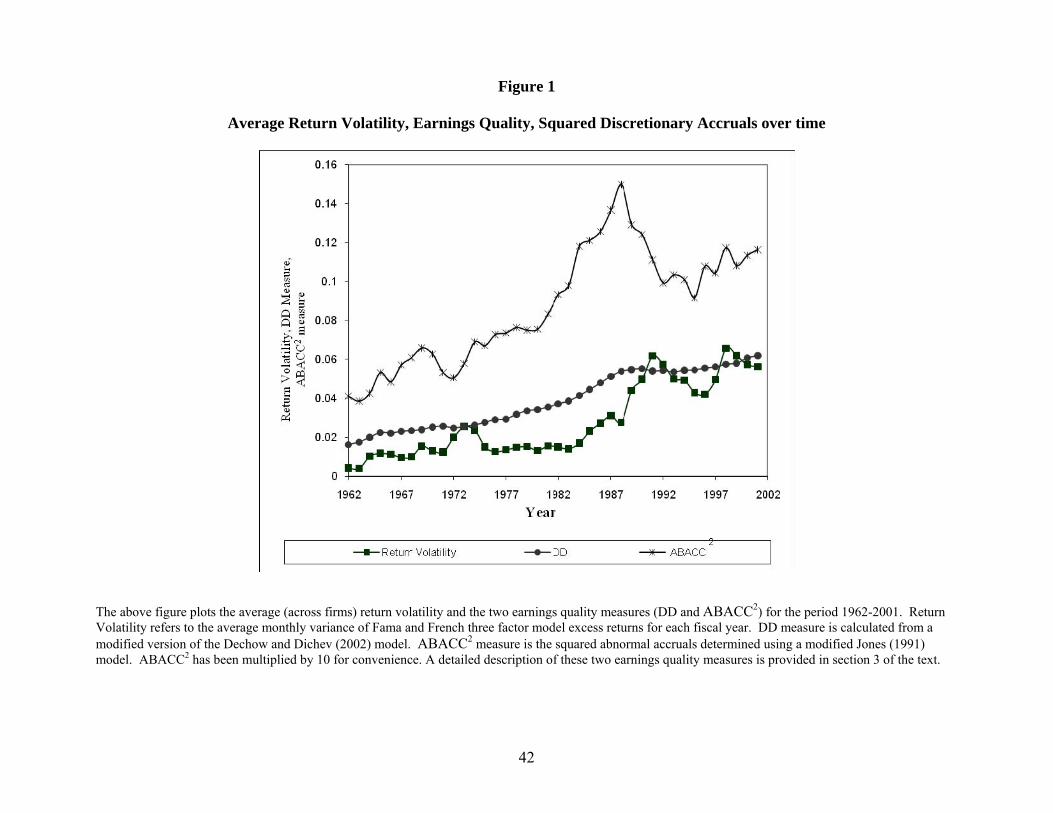
42

Figure 1

Average Return Volatility, Earnings Quality, Squared Discretionary Accruals over time

The above figure plots the average (across firms) return volatility and the two earnings quality measures (DD and ABACC2) for the period 1962-2001. Return Volatility refers to the average monthly variance of Fama and French three factor model excess returns for each fiscal year. DD measure is calculated from a modified version of the Dechow and Dichev (2002) model. ABACC2 measure is the squared abnormal accruals determined using a modified Jones (1991) model. ABACC2 has been multiplied by 10 for convenience. A detailed description of these two earnings quality measures is provided in section 3 of the text.

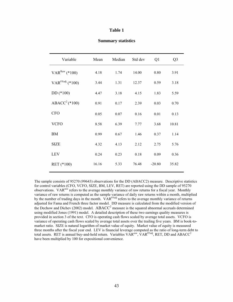
43

Table 1

Summary statistics

Variable Mean Median Std dev Q1 Q3

VARRaw (*100) 4.18 1.74 14.00 0.80 3.91

VARFFadj (*100) 3.44 1.31 12.37 0.59 3.18

DD (*100) 4.47 3.18 4.15 1.83 5.59 ABACC2 (*100) 0.91 0.17 2.39 0.03 0.70 CFO 0.05 0.07 0.16 0.01 0.13 VCFO 8.58 6.39 7.77 3.68 10.81 BM 0.99 0.67 1.46 0.37 1.14 SIZE 4.32 4.13 2.12 2.75 5.76 LEV 0.24 0.23 0.18 0.09 0.36 RET (*100) 16.16 5.33 76.48 -20.80 35.82

The sample consists of 95270 (99643) observations for the DD (ABACC2) measure. Descriptive statistics for control variables (CFO, VCFO, SIZE, BM, LEV, RET) are reported using the DD sample of 95270 observations. VARraw refers to the average monthly variance of raw returns for a fiscal year. Monthly variance of raw returns is computed as the sample variance of daily raw returns within a month, multiplied by the number of trading days in the month. VARFFadj refers to the average monthly variance of returns adjusted for Fama and French three factor model. DD measure is calculated from the modified version of the Dechow and Dichev (2002) model. ABACC2 measure is the squared abnormal accruals determined using modified Jones (1991) model. A detailed description of these two earnings quality measures is provided in section 3 of the text. CFO is operating cash flows scaled by average total assets. VCFO is variance of operating cash flows scaled by average total assets over the trailing five years. BM is book-to-market ratio. SIZE is natural logarithm of market value of equity. Market value of equity is measured three months after the fiscal year end. LEV is financial leverage computed as the ratio of long-term debt to total assets. RET is annual buy-and-hold return. Variables VARraw, VARFFadj, RET, DD and ABACC2 have been multiplied by 100 for expositional convenience.

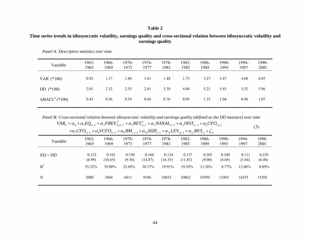
44

Table 2

Time series trends in idiosyncratic volatility, earnings quality and cross-sectional relation between idiosyncratic volatility and earnings quality

Panel A: Descriptive statistics over time

Variable 1962-1965

1966-1969

1970-1973

1974-1977

1978-1981

1982-1985

1986-1989

1990-1993

1994-1997

1998-2001

VAR (*100) 0.92 1.17 1.88 1.61 1.48 1.73 3.27 5.47 4.60 6.03

DD (*100) 2.01 2.32 2.53 2.81 3.38 4.04 5.21 5.43 5.52 5.96

ABACC2 (*100) 0.43 0.56 0.54 0.68 0.76 0.95 1.23 1.04 0.96 1.07

Panel B: Cross-sectional relation between idiosyncratic volatility and earnings quality (defined as the DD measure) over time 2 2

0 1 , 1 2 , , 1 3 , 1 4 , 1 5 , 1 6 , 1

7 , 1 8 , 1 9 , 1 10 1 11 , 1 12 ,

it i t A i t i t i t i t i t

i t i t i t t i t i t it

VAR EQ FREV RET NANAL INST CFO

CFO VCFO BM SIZE LEV RET

(3)

Variable 1962-1965

1966-1969

1970-1973

1974-1977

1978-1981

1982-1985

1986-1989

1990-1993

1994-1997

1998-2001

EQ = DD 0.123 0.101 0.150 0.160 0.124 0.137 0.203 0.240 0.111 0.229

(6.99) (10.65) (9.30) (14.87) (16.33) (11.87) (9.00) (4.69) (3.44) (6.40)

R2 35.32% 39.00% 25.69% 30.37% 19.91% 19.29% 11.26% 8.77% 12.00% 8.89%

N 2000 3804 6811 9196 10853 10062 10599 12485 14255 15205

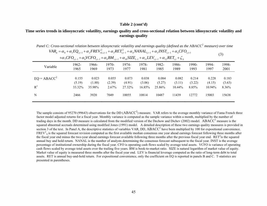
45

Table 2 (cont’d)

Time series trends in idiosyncratic volatility, earnings quality and cross-sectional relation between idiosyncratic volatility and earnings quality

Panel C: Cross-sectional relation between idiosyncratic volatility and earnings quality (defined as the ABACC2 measure) over time 2 2

0 1 , 1 2 , , 1 3 , 1 4 , 1 5 , 1 6 , 1

7 , 1 8 , 1 9 , 1 10 1 11 , 1 12 ,

it i t A i t i t i t i t i t

i t i t i t t i t i t it

VAR EQ FREV RET NANAL INST CFO

CFO VCFO BM SIZE LEV RET

(3)

Variable 1962-1965

1966-1969

1970-1973

1974-1977

1978-1981

1982-1985

1986-1989

1990-1993

1994-1997

1998-2001

EQ = ABACC2 0.155 0.023 0.055 0.073 0.038 0.084 0.082 0.214 0.228 0.183

(5.19) (1.88) (2.39) (4.91) (3.06) (5.27) (3.11) (3.22) (4.15) (3.63) R2 33.32% 35.98% 2.67% 27.32% 16.85% 25.86% 10.44% 8.85% 10.94% 8.36% N 2466 3920 7049 10055 10814 10487 11439 12772 15003 15638

The sample consists of 95270 (99643) observations for the DD (ABACC2) measure. VAR refers to the average monthly variance of Fama French three factor model adjusted returns for a fiscal year. Monthly variance is computed as the sample variance within a month, multiplied by the number of trading days in the month. DD measure is calculated from the modified version of the Dechow and Dichev (2002) model. ABACC2 measure is the squared abnormal accruals determined using modified Jones (1991) model. A detailed description of these two earnings quality measures is provided in section 3 of the text. In Panel A, the descriptive statistics of variables VAR, DD, ABACC2 have been multiplied by 100 for expositional convenience. FREV2

A is the squared forecast revision computed as the first available median consensus one year ahead earnings forecast following three months after the fiscal year end minus the two-year ahead earnings forecast available following three months after the previous fiscal year end. RET2is the squared annual buy and hold return. NANAL is the number of analysts determining the consensus forecast subsequent to the fiscal year. INST is the average percentage of institutional ownership during the fiscal year. CFO is operating cash flows scaled by average total assets. VCFO is variance of operating cash flows scaled by average total assets over the trailing five years. BM is book-to-market ratio. SIZE is natural logarithm of market value of equity. Market value of equity is measured three months after the fiscal year end. LEV is financial leverage computed as the ratio of long-term debt to total assets. RET is annual buy-and-hold return. For expositional convenience, only the coefficient on EQ is reported in panels B and C. T-statistics are presented in parentheses.

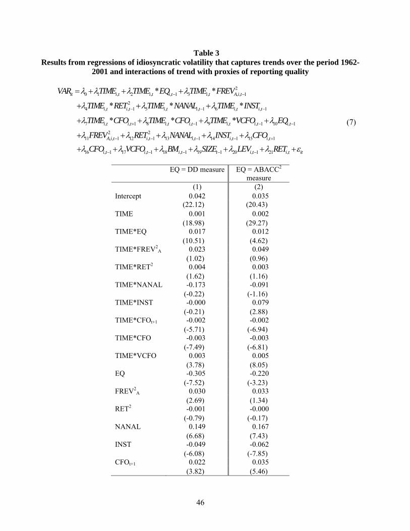
46

Table 3 Results from regressions of idiosyncratic volatility that captures trends over the period 1962-

2001 and interactions of trend with proxies of reporting quality

20 1 , 2 , , 1 3 , , , 1

24 , , 1 5 , , 1 6 , , 1

7 , , 1 8 , , 1 9 , , 1 10 , 1

211 ,

* *

* * *

* * *

it i t i t i t i t A i t

i t i t i t i t i t i t

i t i t i t i t i t i t i t

A

VAR TIME TIME EQ TIME FREV

TIME RET TIME NANAL TIME INST

TIME CFO TIME CFO TIME VCFO EQ

FREV

2, 1 12 , 1 13 , 1 14 , 1 15 , 1

16 , 1 17 , 1 18 , 1 19 1 20 , 1 21 ,

i t i t i t i t i t

i t i t i t t i t i t it

RET NANAL INST CFO

CFO VCFO BM SIZE LEV RET

(7)

EQ = DD measure EQ = ABACC2

measure (1) (2)Intercept 0.042 0.035 (22.12) (20.43)TIME 0.001 0.002 (18.98) (29.27)TIME*EQ 0.017 0.012 (10.51) (4.62)TIME*FREV2

A 0.023 0.049 (1.02) (0.96)TIME*RET2

0.004 0.003 (1.62) (1.16)TIME*NANAL -0.173 -0.091 (-0.22) (-1.16)TIME*INST -0.000 0.079 (-0.21) (2.88)TIME*CFOt+1 -0.002 -0.002 (-5.71) (-6.94)TIME*CFO -0.003 -0.003 (-7.49) (-6.81)TIME*VCFO 0.003 0.005 (3.78) (8.05)EQ -0.305 -0.220 (-7.52) (-3.23)FREV2

A 0.030 0.033 (2.69) (1.34)RET2

-0.001 -0.000 (-0.79) (-0.17)NANAL 0.149 0.167 (6.68) (7.43)INST -0.049 -0.062 (-6.08) (-7.85)CFOt+1 0.022 0.035 (3.82) (5.46)

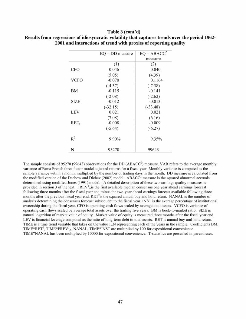
47

Table 3 (cont’d) Results from regressions of idiosyncratic volatility that captures trends over the period 1962-

2001 and interactions of trend with proxies of reporting quality

EQ = DD measure EQ = ABACC2 measure

(1) (2)CFO 0.046 0.040 (5.05) (4.39)VCFO -0.070 0.1164 (-4.37) (-7.38)BM -0.115 -0.141 (-2.08) (-2.62)SIZE -0.012 -0.013 (-32.15) (-33.48)LEV 0.021 0.021 (7.08) (6.16)RETt -0.008 -0.009 (-5.64) (-6.27) R2 9.90% 9.35% N 95270 99643

The sample consists of 95270 (99643) observations for the DD (ABACC2) measure. VAR refers to the average monthly variance of Fama French three factor model adjusted returns for a fiscal year. Monthly variance is computed as the sample variance within a month, multiplied by the number of trading days in the month. DD measure is calculated from the modified version of the Dechow and Dichev (2002) model. ABACC2 measure is the squared abnormal accruals determined using modified Jones (1991) model. A detailed description of these two earnings quality measures is provided in section 3 of the text. FREV2

Ais the first available median consensus one year ahead earnings forecast following three months after the fiscal year end minus the two-year ahead earnings forecast available following three months after the previous fiscal year end. RET2is the squared annual buy and hold return. NANAL is the number of analysts determining the consensus forecast subsequent to the fiscal year. INST is the average percentage of institutional ownership during the fiscal year. CFO is operating cash flows scaled by average total assets. VCFO is variance of operating cash flows scaled by average total assets over the trailing five years. BM is book-to-market ratio. SIZE is natural logarithm of market value of equity. Market value of equity is measured three months after the fiscal year end. LEV is financial leverage computed as the ratio of long-term debt to total assets. RET is annual buy-and-hold return. TIME is a time trend variable that takes on the value 1..N representing each of the years in the sample. Coefficients BM, TIME*RET2, TIME*FREV2

A, NANAL, TIME*INST are multiplied by 100 for expositional convenience. TIME*NANAL has been multiplied by 10000 for expositional convenience. T-statistics are presented in parentheses.

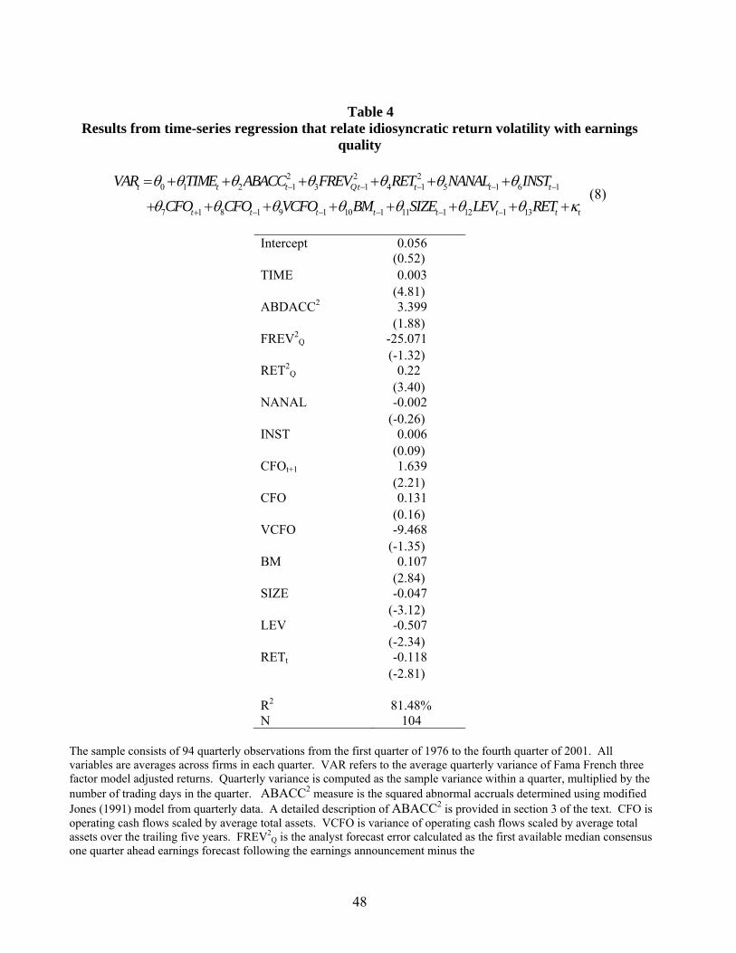
48

Table 4

Results from time-series regression that relate idiosyncratic return volatility with earnings quality

2 2 2

0 1 2 1 3 1 4 1 5 1 6 1

7 1 8 1 9 1 10 1 11 1 12 1 13

t t t Qt t t t

t t t t t t t t

VAR TIME ABACC FREV RET NANAL INST

CFO CFO VCFO BM SIZE LEV RET

(8)

Intercept 0.056 (0.52)TIME 0.003 (4.81)ABDACC2 3.399 (1.88)FREV2

Q -25.071 (-1.32)RET2

Q 0.22 (3.40)NANAL -0.002 (-0.26)INST 0.006 (0.09)CFOt+1 1.639 (2.21)CFO 0.131 (0.16)VCFO -9.468 (-1.35)BM 0.107 (2.84)SIZE -0.047 (-3.12)LEV -0.507 (-2.34)RETt -0.118 (-2.81) R2 81.48%N 104

The sample consists of 94 quarterly observations from the first quarter of 1976 to the fourth quarter of 2001. All variables are averages across firms in each quarter. VAR refers to the average quarterly variance of Fama French three factor model adjusted returns. Quarterly variance is computed as the sample variance within a quarter, multiplied by the number of trading days in the quarter. ABACC2 measure is the squared abnormal accruals determined using modified Jones (1991) model from quarterly data. A detailed description of ABACC2 is provided in section 3 of the text. CFO is operating cash flows scaled by average total assets. VCFO is variance of operating cash flows scaled by average total assets over the trailing five years. FREV2

Q is the analyst forecast error calculated as the first available median consensus one quarter ahead earnings forecast following the earnings announcement minus the

49

Table 4 (cont’d)

Results from time-series regression that relate idiosyncratic return volatility with earnings quality

first available two quarter ahead consensus earnings forecast available following the previous earnings announcement scaled by the stock price at that date. RET2 is the squared quarterly buy and hold return. RET is quarterly buy-and-hold return. TIME is a time trend variable that takes on the value from 1 to 104 representing each of the quarters in the sample. All the other variables have been defined in notes to Table 3. T-statistics are presented in parentheses.

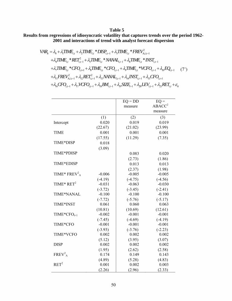
50

Table 5 Results from regressions of idiosyncratic volatility that captures trends over the period 1962-

2001 and interactions of trend with analyst forecast dispersion

20 1 , 2 , , 1 3 , , , 1

24 , , 1 5 , , 1 6 , , 1

7 , , 1 8 , , 1 9 , , 1 10 , 1

11

* *

* * *

* * *

it i t i t i t i t A i t

i t i t i t i t i t i t

i t i t i t i t i t i t i t

A

VAR TIME TIME DISP TIME FREV

TIME RET TIME NANAL TIME INST

TIME CFO TIME CFO TIME VCFO EQ

FREV

2 2, , 1 12 , 1 13 , 1 14 , 1 15 , 1

16 , 1 17 , 1 18 , 1 19 1 20 , 1 21 ,

i t i t i t i t i t

i t i t i t t i t i t it

RET NANAL INST CFO

CFO VCFO BM SIZE LEV RET

(7’)

EQ = DD measure

EQ = ABACC2 measure

(1) (2) (3) Intercept 0.020 0.019 0.019 (22.67) (21.02) (23.99) TIME 0.001 0.001 0.001 (17.55) (11.29) (7.35) TIME*DISP 0.018 (3.09) TIME*PDISP 0.083 0.020 (2.73) (1.86) TIME*EDISP 0.013 0.013 (2.37) (1.98) TIME* FREV2

A -0.006 -0.005 -0.005 (-4.19) (-4.75) (-4.56) TIME* RET2 -0.031 -0.063 -0.030 (-3.72) (-3.45) (-2.41) TIME*NANAL -0.100 -0.100 -0.100 (-7.72) (-5.76) (-5.17) TIME*INST 0.061 0.060 0.063 (10.81) (10.69) (12.61) TIME*CFOt+1 -0.002 -0.001 -0.001 (-7.45) (-4.69) (-4.19) TIME*CFO -0.001 -0.001 -0.001 (-3.93) (-3.76) (-2.23) TIME*VCFO 0.002 0.002 0.002 (5.12) (3.95) (3.07) DISP 0.002 0.002 0.002 (1.95) (2.62) (2.58) FREV2

A 0.174 0.149 0.143 (4.89) (5.28) (4.83) RET2 0.001 0.002 0.003 (2.26) (2.96) (2.33)

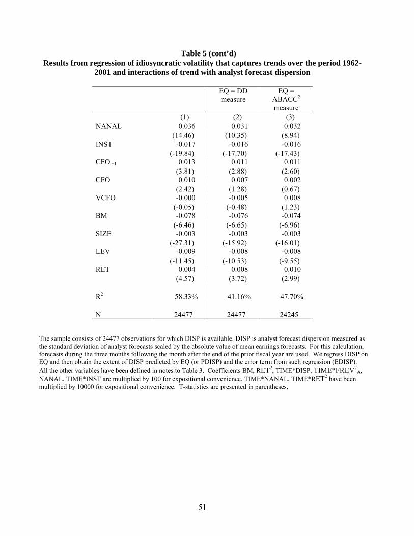
51

Table 5 (cont’d) Results from regression of idiosyncratic volatility that captures trends over the period 1962-

2001 and interactions of trend with analyst forecast dispersion

EQ = DD measure

EQ = ABACC2 measure

(1) (2) (3) NANAL 0.036 0.031 0.032 (14.46) (10.35) (8.94) INST -0.017 -0.016 -0.016 (-19.84) (-17.70) (-17.43) CFOt+1 0.013 0.011 0.011 (3.81) (2.88) (2.60) CFO 0.010 0.007 0.002 (2.42) (1.28) (0.67) VCFO -0.000 -0.005 0.008 (-0.05) (-0.48) (1.23) BM -0.078 -0.076 -0.074 (-6.46) (-6.65) (-6.96) SIZE -0.003 -0.003 -0.003 (-27.31) (-15.92) (-16.01) LEV -0.009 -0.008 -0.008 (-11.45) (-10.53) (-9.55) RET 0.004 0.008 0.010 (4.57) (3.72) (2.99) R2 58.33% 41.16% 47.70% N 24477 24477 24245

The sample consists of 24477 observations for which DISP is available. DISP is analyst forecast dispersion measured as the standard deviation of analyst forecasts scaled by the absolute value of mean earnings forecasts. For this calculation, forecasts during the three months following the month after the end of the prior fiscal year are used. We regress DISP on EQ and then obtain the extent of DISP predicted by EQ (or PDISP) and the error term from such regression (EDISP). All the other variables have been defined in notes to Table 3. Coefficients BM, RET2, TIME*DISP, TIME*FREV2

A, NANAL, TIME*INST are multiplied by 100 for expositional convenience. TIME*NANAL, TIME*RET2 have been multiplied by 10000 for expositional convenience. T-statistics are presented in parentheses.

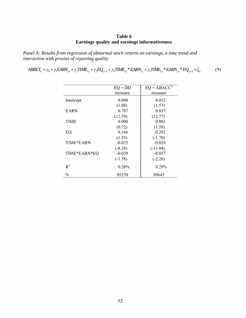
52

Table 6

Earnings quality and earnings informativeness

Panel A: Results from regression of abnormal stock returns on earnings, a time trend and interaction with proxies of reporting quality

0 1 , 2 , 3 , 1 4 , , 5 , , , 1* * *it i t i t i t i t i t i t i t i t itABRET EARN TIME EQ TIME EARN TIME EARN EQ (9)

EQ = DD measure

EQ = ABACC2 measure

Intercept 0.008 0.012 (1.08) (1.53)EARN 0.787 0.857 (12.59) (12.77)TIME 0.000 0.001 (0.72) (1.58)EQ 0.166 -0.282 (1.55) (-1.70)TIME*EARN -0.025 -0.029 (-8.28) (-11.04)TIME*EARN*EQ -0.039 -0.057 (-1.58) (-2.26)

R2 0.28% 0.29%

N 95270 99643

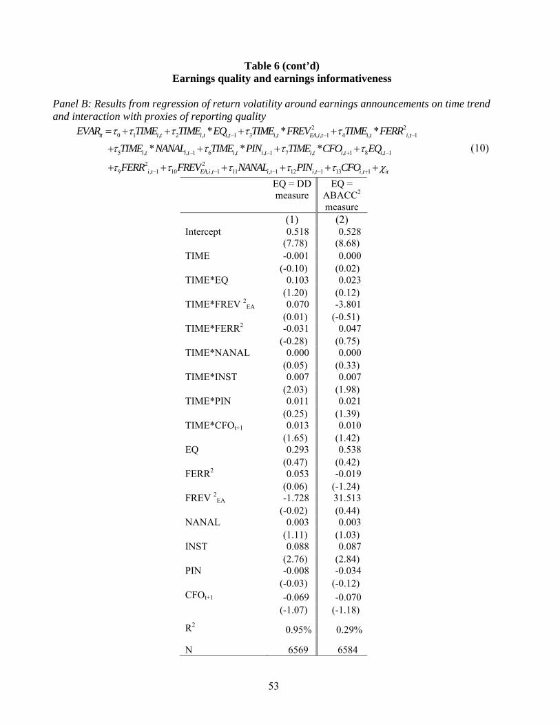
53

Table 6 (cont’d) Earnings quality and earnings informativeness

Panel B: Results from regression of return volatility around earnings announcements on time trend and interaction with proxies of reporting quality

2 20 1 , 2 , , 1 3 , , , 1 4 , , 1

5 , , 1 6 , , 1 7 , , 1 8 , 1

2 29 , 1 10 , , 1 11 , 1 12

* * *

* * *it i t i t i t i t EA i t i t i t

i t i t i t i t i t i t i t

i t EA i t i t

EVAR TIME TIME EQ TIME FREV TIME FERR

TIME NANAL TIME PIN TIME CFO EQ

FERR FREV NANAL P

, 1 13 , 1i t i t itIN CFO

(10)

EQ = DD measure

EQ = ABACC2 measure

(1) (2) Intercept 0.518 0.528 (7.78) (8.68)TIME -0.001 0.000 (-0.10) (0.02)TIME*EQ 0.103 0.023 (1.20) (0.12)TIME*FREV 2EA 0.070 -3.801 (0.01) (-0.51)TIME*FERR2 -0.031 0.047 (-0.28) (0.75)TIME*NANAL 0.000 0.000 (0.05) (0.33)TIME*INST 0.007 0.007 (2.03) (1.98)TIME*PIN 0.011 0.021 (0.25) (1.39)TIME*CFOt+1 0.013 0.010 (1.65) (1.42)EQ 0.293 0.538 (0.47) (0.42)FERR2 0.053 -0.019 (0.06) (-1.24)FREV 2EA -1.728 31.513 (-0.02) (0.44)NANAL 0.003 0.003 (1.11) (1.03)INST 0.088 0.087 (2.76) (2.84)PIN -0.008 -0.034 (-0.03) (-0.12)CFOt+1 -0.069 -0.070 (-1.07) (-1.18)

R2 0.95% 0.29%

N 6569 6584

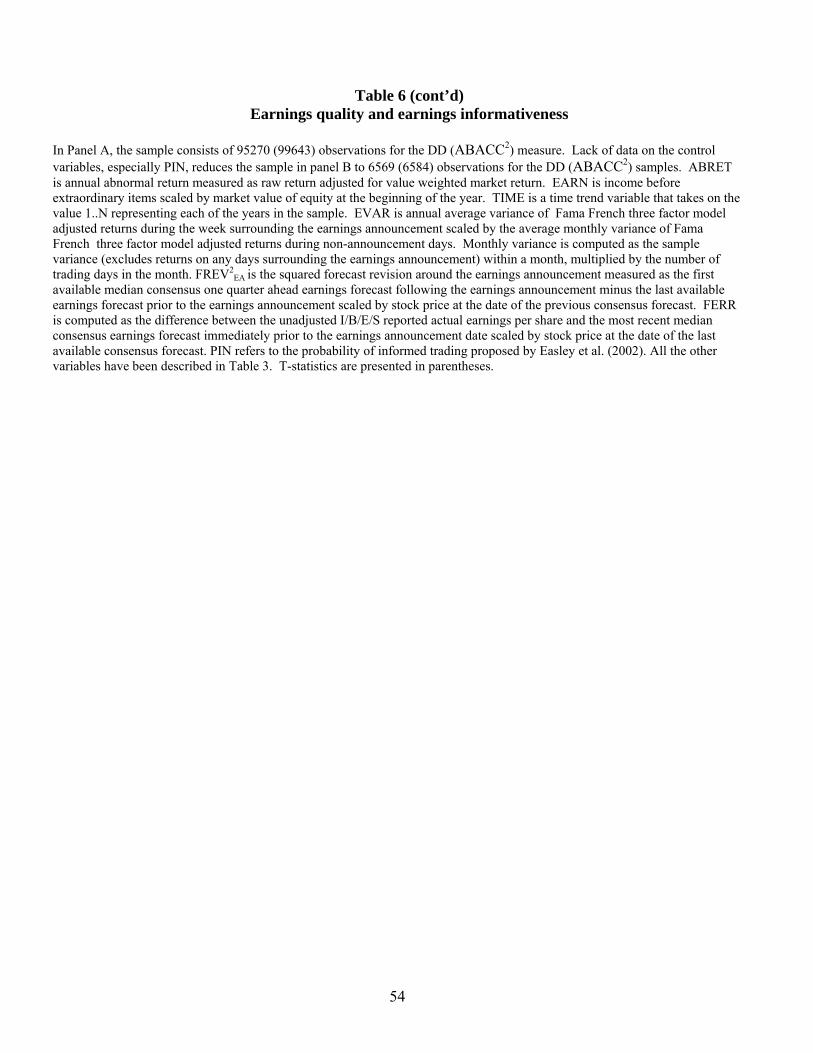
54

Table 6 (cont’d) Earnings quality and earnings informativeness

In Panel A, the sample consists of 95270 (99643) observations for the DD (ABACC2) measure. Lack of data on the control variables, especially PIN, reduces the sample in panel B to 6569 (6584) observations for the DD (ABACC2) samples. ABRET is annual abnormal return measured as raw return adjusted for value weighted market return. EARN is income before extraordinary items scaled by market value of equity at the beginning of the year. TIME is a time trend variable that takes on the value 1..N representing each of the years in the sample. EVAR is annual average variance of Fama French three factor model adjusted returns during the week surrounding the earnings announcement scaled by the average monthly variance of Fama French three factor model adjusted returns during non-announcement days. Monthly variance is computed as the sample variance (excludes returns on any days surrounding the earnings announcement) within a month, multiplied by the number of trading days in the month. FREV2

EA is the squared forecast revision around the earnings announcement measured as the first available median consensus one quarter ahead earnings forecast following the earnings announcement minus the last available earnings forecast prior to the earnings announcement scaled by stock price at the date of the previous consensus forecast. FERR is computed as the difference between the unadjusted I/B/E/S reported actual earnings per share and the most recent median consensus earnings forecast immediately prior to the earnings announcement date scaled by stock price at the date of the last available consensus forecast. PIN refers to the probability of informed trading proposed by Easley et al. (2002). All the other variables have been described in Table 3. T-statistics are presented in parentheses.

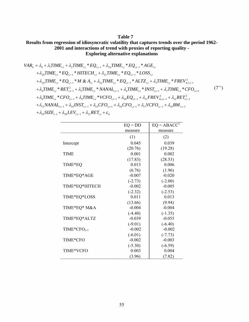
55

Table 7

Results from regression of idiosyncratic volatility that captures trends over the period 1962-2001 and interactions of trend with proxies of reporting quality -

Exploring alternative explanations

0 1 , 2 , , 1 2 , , 1 ,

2 , , 1 , 2 , , 1 ,

22 , , 1 , 2 , , 1 , 3 , , , 1

4

* * *

* * * *

* * & * * *

it i t i t i t a i t i t i t

b i t i t i t c i t i t i t

d i t i t i t e i t i t i t i t A i t

VAR TIME TIME EQ TIME EQ AGE

TIME EQ HITECH TIME EQ LOSS

TIME EQ M A TIME EQ ALTZ TIME FREV

TIM

2, , 1 5 , , 1 6 , , 1 7 , , 1

2 28 , , 1 9 , , 1 10 , 1 11 , , 1 12 , 1

13 , 1 14 , 1 15 , 1 16

* * * *

* *

i t i t i t i t i t i t i t i t

i t i t i t i t i t A i t i t

i t i t i t i

E RET TIME NANAL TIME INST TIME CFO

TIME CFO TIME VCFO EQ FREV RET

NANAL INST CFO CFO

, 1 17 , 1 18 , 1

19 1 20 , 1 21 ,

t i t i t

t i t i t it

VCFO BM

SIZE LEV RET

(7’’)

EQ = DD

measureEQ = ABACC2

measure (1) (2) Intercept 0.045 0.039 (20.76) (19.28)TIME 0.001 0.002 (17.83) (28.53)TIME*EQ 0.013 0.006 (6.76) (1.96)TIME*EQ*AGE -0.007 -0.020 (-2.73) (-2.00)TIME*EQ*HITECH -0.002 -0.005 (-2.32) (-2.53)TIME*EQ*LOSS 0.011 0.013 (13.66) (9.94)TIME*EQ* M&A -0.004 -0.004 (-4.40) (-1.35)TIME*EQ*ALTZ -0.039 -0.055 (-9.01) (-6.40)TIME*CFOt+1 -0.002 -0.002 (-6.01) (-7.73)TIME*CFO -0.002 -0.003 (-5.30) (-6.59)TIME*VCFO 0.003 0.004 (3.96) (7.82)

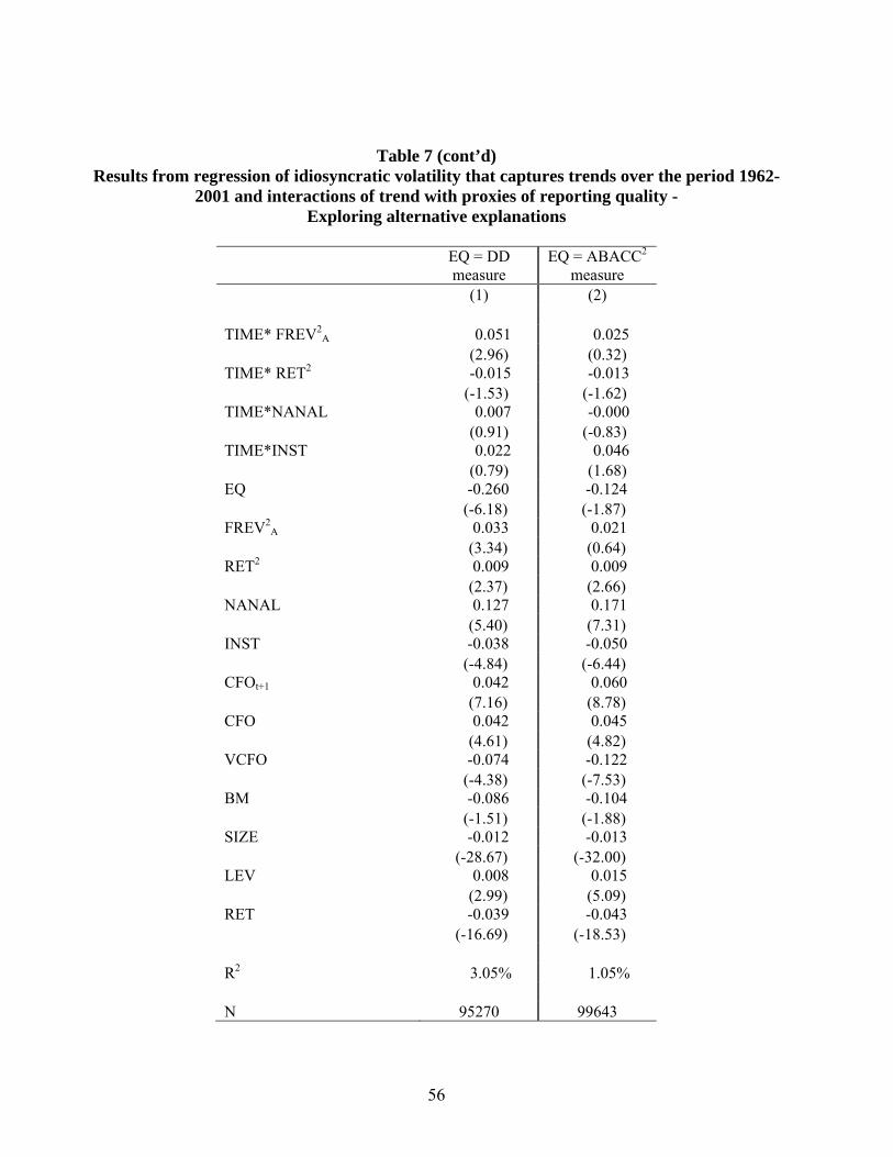
56

Table 7 (cont’d) Results from regression of idiosyncratic volatility that captures trends over the period 1962-

2001 and interactions of trend with proxies of reporting quality - Exploring alternative explanations

EQ = DD

measureEQ = ABACC2

measure (1) (2) TIME* FREV2

A 0.051 0.025 (2.96) (0.32) TIME* RET2 -0.015 -0.013 (-1.53) (-1.62) TIME*NANAL 0.007 -0.000 (0.91) (-0.83) TIME*INST 0.022 0.046 (0.79) (1.68) EQ -0.260 -0.124 (-6.18) (-1.87)FREV2

A 0.033 0.021 (3.34) (0.64)RET2 0.009 0.009 (2.37) (2.66)NANAL 0.127 0.171 (5.40) (7.31)INST -0.038 -0.050 (-4.84) (-6.44)CFOt+1 0.042 0.060 (7.16) (8.78)CFO 0.042 0.045 (4.61) (4.82)VCFO -0.074 -0.122 (-4.38) (-7.53)BM -0.086 -0.104 (-1.51) (-1.88)SIZE -0.012 -0.013 (-28.67) (-32.00)LEV 0.008 0.015 (2.99) (5.09)RET -0.039 -0.043 (-16.69) (-18.53) R2 3.05% 1.05% N 95270 99643

57

Table 7 (cont’d) Results from regression of idiosyncratic volatility that captures trends over the period 1962-

2001 and interactions of trend with proxies of reporting quality – Exploring alternative explanations

The sample consists of 95270 (99643) observations for the DD (ABACC2) measure. Refer to notes at the bottom of Table 3 for definitions of the variables used here. The new variables in this table are as follows. AGE is defined as the number of years since the first day for which we can find a stock price in the CRSP tapes, HITECH is a dummy variable that is set to one (zero otherwise) if the firm-year belongs to the high technology SIC codes, LOSS is a dummy variable that is set to one (zero otherwise) if the firm-year reports negative earnings. M&A is a dummy variable that is set to one (zero otherwise) if firms have either experienced M&A transactions as reported in COMPUSTAT annual footnote code #1 or divestitures (COMPUSTAT data item 66) or foreign currency translations (COMPUSTAT data item 150). ALTZ is Altman Z score computed using COMPUSTAT data as follows: ALTZ = 1.2 * (data179/data6) + 1.4* (data36/data6) + 3.3 *(data18+data16+data15)/data6 + 0.6 * (data199*data25)/data181 +data12/data6. Coefficients BM, TIME*EQ*AGE, TIME*EQ*ALTZ, TIME* RET2, TIME*FREV2

A, NANAL, TIME*INST are multiplied by 100 for expositional convenience. TIME*NANAL has been multiplied by 10000 for expositional convenience. T-statistics are presented in parentheses.

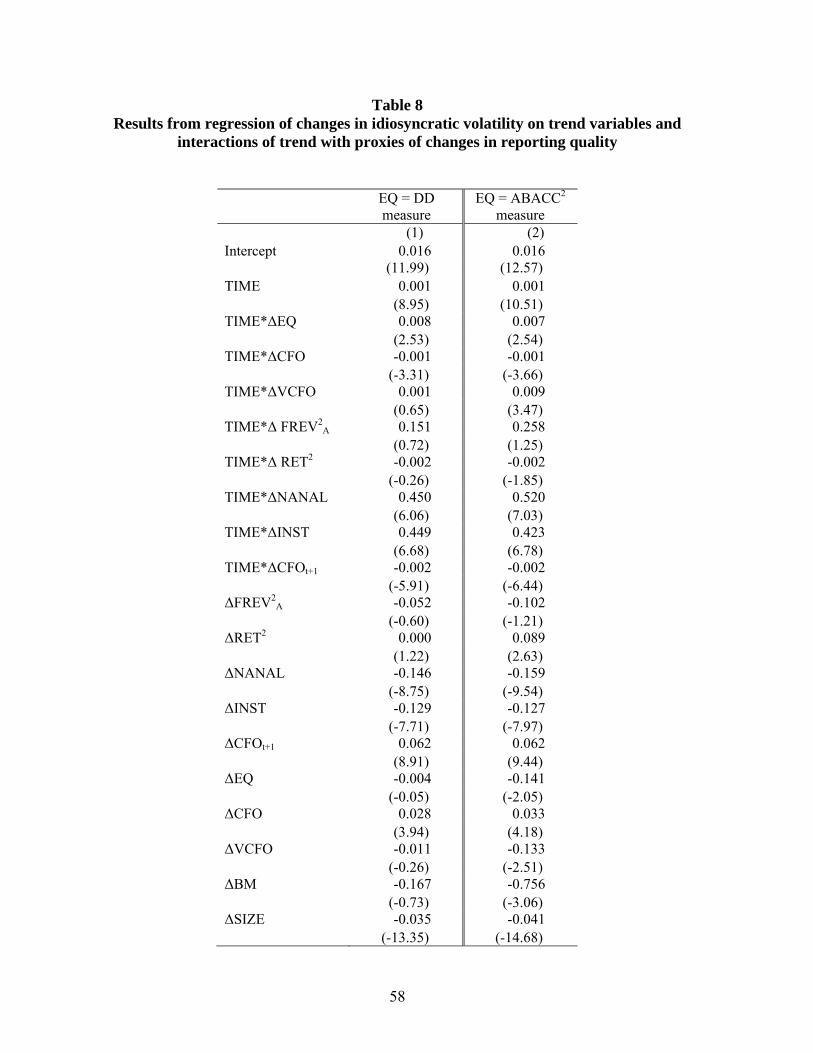
58

Table 8 Results from regression of changes in idiosyncratic volatility on trend variables and

interactions of trend with proxies of changes in reporting quality

EQ = DD measure

EQ = ABACC2 measure

(1) (2)Intercept 0.016 0.016 (11.99) (12.57)TIME 0.001 0.001 (8.95) (10.51)TIME*ΔEQ 0.008 0.007 (2.53) (2.54)TIME*ΔCFO -0.001 -0.001 (-3.31) (-3.66)TIME*ΔVCFO 0.001 0.009 (0.65) (3.47)TIME*Δ FREV2

A 0.151 0.258 (0.72) (1.25)TIME*Δ RET2 -0.002 -0.002 (-0.26) (-1.85)TIME*ΔNANAL 0.450 0.520 (6.06) (7.03)TIME*ΔINST 0.449 0.423 (6.68) (6.78)TIME*ΔCFOt+1 -0.002 -0.002 (-5.91) (-6.44)ΔFREV2

A -0.052 -0.102 (-0.60) (-1.21)ΔRET2 0.000 0.089 (1.22) (2.63)ΔNANAL -0.146 -0.159 (-8.75) (-9.54)ΔINST -0.129 -0.127 (-7.71) (-7.97)ΔCFOt+1 0.062 0.062 (8.91) (9.44)ΔEQ -0.004 -0.141 (-0.05) (-2.05)ΔCFO 0.028 0.033 (3.94) (4.18)ΔVCFO -0.011 -0.133 (-0.26) (-2.51)ΔBM -0.167 -0.756 (-0.73) (-3.06)ΔSIZE -0.035 -0.041 (-13.35) (-14.68)

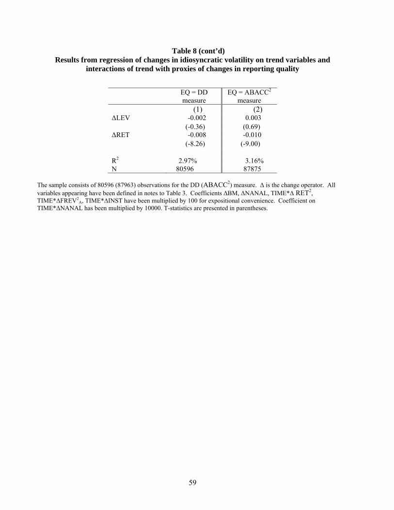
59

Table 8 (cont’d) Results from regression of changes in idiosyncratic volatility on trend variables and

interactions of trend with proxies of changes in reporting quality

EQ = DD measure

EQ = ABACC2 measure

(1) (2) ΔLEV -0.002 0.003 (-0.36) (0.69)ΔRET -0.008 -0.010 (-8.26) (-9.00) R2 2.97% 3.16%N 80596 87875

The sample consists of 80596 (87963) observations for the DD (ABACC2) measure. Δ is the change operator. All variables appearing have been defined in notes to Table 3. Coefficients ΔBM, ΔNANAL, TIME*Δ RET2, TIME*ΔFREV2

A, TIME*ΔINST have been multiplied by 100 for expositional convenience. Coefficient on TIME*ΔNANAL has been multiplied by 10000. T-statistics are presented in parentheses.