hw6: routing - solutions

HW6: Routing - SolutionsCOM-208: Computer Networks

Link-state routing

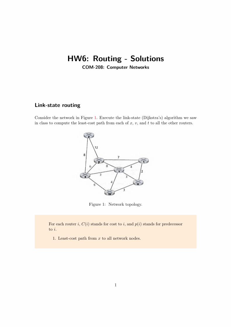
Consider the network in Figure 1. Execute the link-state (Dijkstra’s) algorithm we sawin class to compute the least-cost path from each of x, v, and t to all the other routers.

Figure 1: Network topology.

For each router i, C(i) stands for cost to i, and p(i) stands for predecessorto i.

1. Least-cost path from x to all network nodes.

1

step nodes visited C(t),p(t) C(u),p(u) C(v),p(v) C(w),p(w) C(y),p(y) C(z),p(z)0 x ∞ ∞ 3,x 6,x 6,x 8,x1 x,v 7,v 6,v 3,x 6,x 6,x 8,x2 x,v,u 7,v 6,v 3,x 6,x 6,x 8,x3 x,v,u,w 7,v 6,v 3,x 6,x 6,x 8,x4 x,v,u,w,y 7,v 6,v 3,x 6,x 6,x 8,x5 x,v,u,w,y,t 7,v 6,v 3,x 6,x 6,x 8,x6 x,v,u,w,y,t,z 7,v 6,v 3,x 6,x 6,x 8,x

2. Least-cost path from v to all network nodes.

step nodes visited C(t),p(t) C(u),p(u) C(w),p(w) C(x),p(x) C(y),p(y) C(z),p(z)0 v 4,v 3,v 4,v 3,v 8,v ∞1 v,x 4,v 3,v 4,v 3,v 8,v 11,x2 v,x,u 4,v 3,v 4,v 3,v 8,v 11,x3 v,x,u,t 4,v 3,v 4,v 3,v 8,v 11,x4 v,x,u,t,w 4,v 3,v 4,v 3,v 8,v 11,x5 v,x,u,t,w,y 4,v 3,v 4,v 3,v 8,v 11,x6 v,x,u,t,w,y,z 4,v 3,v 4,v 3,v 8,v 11,x

3. Least-cost path from t to all network nodes.

step nodes visited C(u),p(u) C(v),p(v) C(w),p(w) C(x),p(x) C(y),p(y) C(z),p(z)0 t 2,t 4,t ∞ ∞ 7,t ∞1 t,u 2,t 4,t 5,u ∞ 7,t ∞2 t,u,v 2,t 4,t 5,u 7,v 7,t ∞3 t,u,v,w 2,t 4,t 5,u 7,v 7,t ∞4 t,u,v,w,x 2,t 4,t 5,u 7,v 7,t 15,x5 t,u,v,w,x,y 2,t 4,t 5,u 7,v 7,t 15,x6 t,u,v,w,x,y,z 2,t 4,t 5,u 7,v 7,t 15,x

2

Distance-vector routing

Consider the network in Figure 2. Execute the distance-vector (Bellman-Ford) algorithmwe saw in class and show the information that router z knows after each iteration.


Each node in the topology has its own view of the network, which isupdated independently from other nodes at the end of each step. Therefore,for every step of the algorithm, you also need to update each of the othercost tables. Otherwise, your solution may be incorrect.

In our solution we only show the cost table for node z, as required bythe question. The cost table at node z consists of 5 columns (all possibledestinations) and 3 rows (all possible sources—one row for node z and onerow for each neighbor). Each entry of the table denotes the cost betweenthe associated source-destination nodes.

Initially (at step 0), node z has the following view of the network:

Tou v x y z

Fromv ∞ ∞ ∞ ∞ ∞x ∞ ∞ ∞ ∞ ∞z ∞ 6 2 ∞ 0

At step 1:

Tou v x y z

Fromv 1 0 3 ∞ 6x ∞ 3 0 3 2z 7 5 2 5 0

3

At step 2:

Tou v x y z

Fromv 1 0 3 3 5x 4 3 0 3 2z 6 5 2 5 0

At step 3:

Tou v x y z

Fromv 1 0 3 3 5x 4 3 0 3 2z 6 5 2 5 0

We see that from step 2 to step 3 the cost tables did not change, indicatingthat the algorithm has converged.

Convergence

What is the maximum number of iterations required for the distance-vector (Bellman-Ford) algorithm that we saw in class to converge (i.e., to finish, assuming no changeoccurs in the network graph and link costs)? Justify your answer.

At each iteration, a node exchanges cost tables with its neighbors. Thus,if you are node A, and your neighbor is B, all of B’s neighbors (which areall one or two hops from you) will know the least-cost path of one or twohops to you after one iteration (i.e., after B tells them its cost to you).

Let d be the “diameter” of the network, which is computed as follows:

• Find the least-cost path between each pair of nodes.

• The diameter is equal to the greatest length (in number of links) ofany of those least-cost paths.

Using the reasoning above, after d− 1 iterations, all nodes will know theleast-cost path of cost ≤ d hops to all other nodes. Since any path of cost> d hops is longer (and costlier) than any of the least-cost paths, thealgorithm converges in at most d− 1 iterations.

4

Poisoned reverse

Consider the network in Figure 3. The routers in the network run the distance-vector(Bellman-Ford) algorithm we saw in class, with poisoned reverse enabled. Suppose thealgorithm has run for some time and has converged to the correct least-cost paths.

Table 4 contains the reachability information from each router to router A (e.g., fromrouter D we can reach router A through router C with cost 3).

Now suppose that link A−B goes down.

1

1

1

1

2

A

C

B

E

D


Describe the next 6 steps of the algorithm. For each step, show the reachability informationfrom each router to router A (cost of the least-cost path and next hop).

See Figures 4 and 5.

To fill in the first table we use the second, auxiliary one: Figure 5 shows therouting announcements exchanged between routers and the computationsdone to update the routing tables. Only the information relevant to routesto router A is shown. At each step, each router sends to its neighbors thebest route to A known in the previous step, except if the route is via thatneighbor, in which case because of poisoned reverse, ∞ is sent; we marksuch messages with (pr). Then, each router uses all the announcementsit received from the neighbors to update its routing table.

Note that poisoned reverse does not help the algorithm converge.

5

from router B from router C from router D from router Erouteto

router

A step 0 1 via A 2 via B 3 via C 3 via Bstep 1 ∞ 2 via B 3 via C 3 via Bstep 2 ∞ ∞ 3 via C 4 via Dstep 3 6 via E ∞ ∞ 4 via Dstep 4 6 via E 7 via B ∞ ∞step 5 ∞ 7 via B 8 via C ∞step 6 ∞ ∞ 8 via C 9 via D

Figure 4: Reachability information from each router to router A.

6

router B router C router D router Estep

0

initial table 1 via A 2 via B 3 via C 3 via B

step

1

C → B :∞ (pr) B → C : 1 C → D : 2 B → E : 1announcements E → B :∞ (pr) D → C :∞ (pr) E → D : 3 D → E : 3

link to A downtable update ∞ 1 + 1 = 2 via B 2 + 1 = 3 via C 1 + 2 = 3 via B

step

2

C → B :∞ (pr) B → C :∞ C → D : 2 B → E :∞announcements E → B :∞ (pr) D → C :∞ (pr) E → D : 3 D → E : 3

link to A downtable update ∞ ∞ 2 + 1 = 3 via C 3 + 1 = 4 via D

step

3

C → B :∞ B → C :∞ C → D :∞ B → E :∞announcements E → B : 4 D → C :∞ (pr) E → D :∞ (pr) D → E : 3

link to A downtable update 4 + 2 = 6 via E ∞ ∞ 3 + 1 = 4 via D

step

4

C → B :∞ B → C : 6 C → D :∞ B → E :∞ (pr)announcements E → B : 4 D → C :∞ E → D :∞ (pr) D → E :∞

link to A downtable update 4 + 2 = 6 via E 6 + 1 = 7 via B ∞ ∞

step

5

C → B :∞ (pr) B → C : 6 C → D : 7 B → E :∞ (pr)announcements E → B :∞ D → C :∞ E → D :∞ D → E :∞

link to A downtable update ∞ 6 + 1 = 7 via B 7 + 1 = 8 via C ∞

step

6

C → B :∞ (pr) B → C :∞ C → D : 7 B → E :∞announcements E → B :∞ D → C :∞ (pr) E → D :∞ D → E : 8

link to A downtable update ∞ ∞ 7 + 1 = 8 via C 8 + 1 = 9 via D

Figure 5: Routing announcements exchanged between routers and routing tableupdates.

7

Will the algorithm converge to the correct least-cost path values? If yes, in how manysteps?

No, the algorithm does not converge (the algorithm takes an infinitenumber of steps to converge to the correct least-cost path values).

Propose a simple way to make the algorithm converge faster.

Potential solutions:

• Routers keep track of the entire route-path, not just the next hop(e.g., BGP)

• Routers use an upper limit for the cost of a path (e.g., 30). Thealgorithm converges slowly, but will eventually converge.

8

Put forwarding and routing together

Consider the network in Figure 6, consisting of:

• End-systems A, B and X, DNS server C, and web server D.

• IP routers R1, R2, R3, and R4.

• The link costs are noted in Figure 6.

• End-systems A, B and X use C as their local DNS server.

End-system A

End-system B

End-system XDNS Server C

Web Server Dwww.epfl.ch


IP prefix/address allocation

Allocate an IP prefix to each IP subnet and an IP address to each network interface thatneeds one, following these rules:

• All IP addresses must be allocated from 8.8.8.0/24.

• Each IP subnet must be allocated the smallest possible IP prefix and must haveone broadcast IP address.

• IP router interfaces have IP addresses.

9

Explain how you compute each IP prefix and fill in Table 7.

Subnet number IP prefix Interfaces and IP addresses Broadcast IP addressExample: 1 10.1.1.0/24 x: 10.1.1.0 10.1.1.255

y: 10.1.1.1z: 10.1.1.2

1 8.8.8.0/29 a : 8.8.8.0 8.8.8.7b : 8.8.8.1x : 8.8.8.2h : 8.8.8.3

2 8.8.8.8/30 c : 8.8.8.8 8.8.8.11d : 8.8.8.9s : 8.8.8.10

3 8.8.8.12/30 o : 8.8.8.12 8.8.8.15p : 8.8.8.13

4 8.8.8.16/30 q : 8.8.8.16 8.8.8.19r : 8.8.8.17

5 8.8.8.20/30 k : 8.8.8.20 8.8.8.23l : 8.8.8.21

6 8.8.8.24/30 i : 8.8.8.24 8.8.8.27j : 8.8.8.25

7 8.8.8.28/30 n : 8.8.8.28 8.8.8.31m : 8.8.8.29

Figure 7: Allocation of IP prefixes and IP addresses for the network in Figure 6.

10

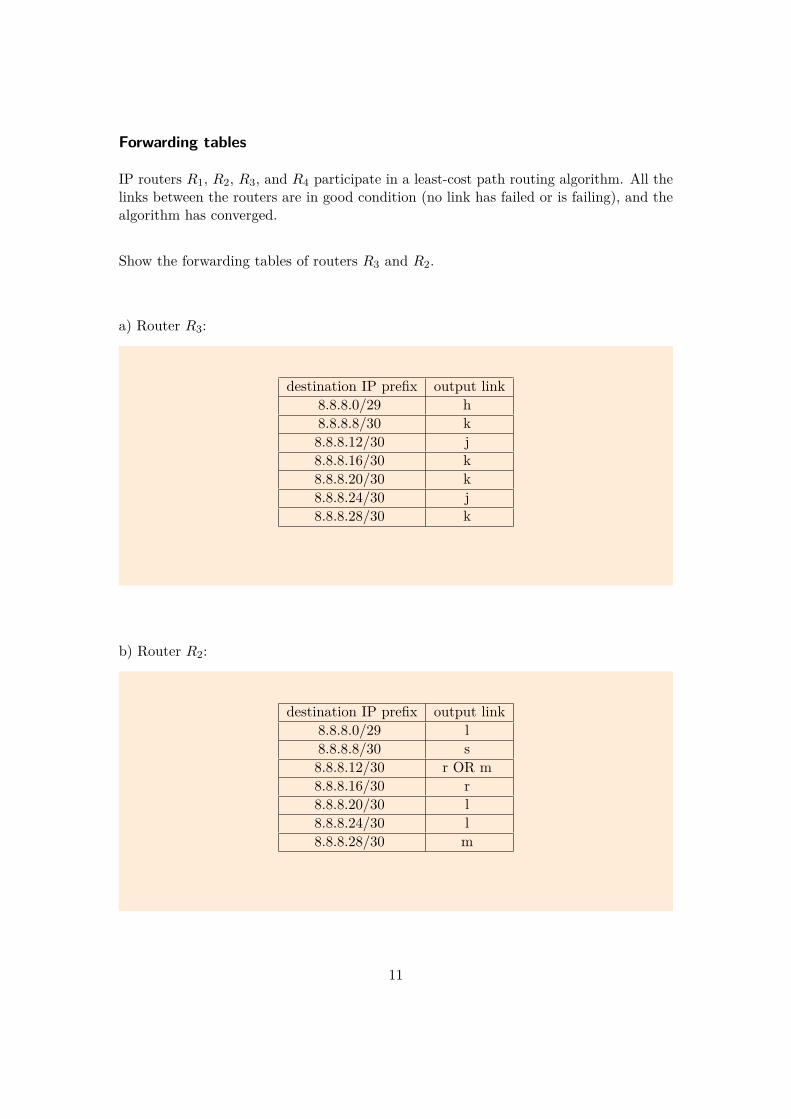
Forwarding tables

IP routers R1, R2, R3, and R4 participate in a least-cost path routing algorithm. All thelinks between the routers are in good condition (no link has failed or is failing), and thealgorithm has converged.

Show the forwarding tables of routers R3 and R2.

a) Router R3:

destination IP prefix output link8.8.8.0/29 h8.8.8.8/30 k8.8.8.12/30 j8.8.8.16/30 k8.8.8.20/30 k8.8.8.24/30 j8.8.8.28/30 k

b) Router R2:

destination IP prefix output link8.8.8.0/29 l8.8.8.8/30 s8.8.8.12/30 r OR m8.8.8.16/30 r8.8.8.20/30 l8.8.8.24/30 l8.8.8.28/30 m

11

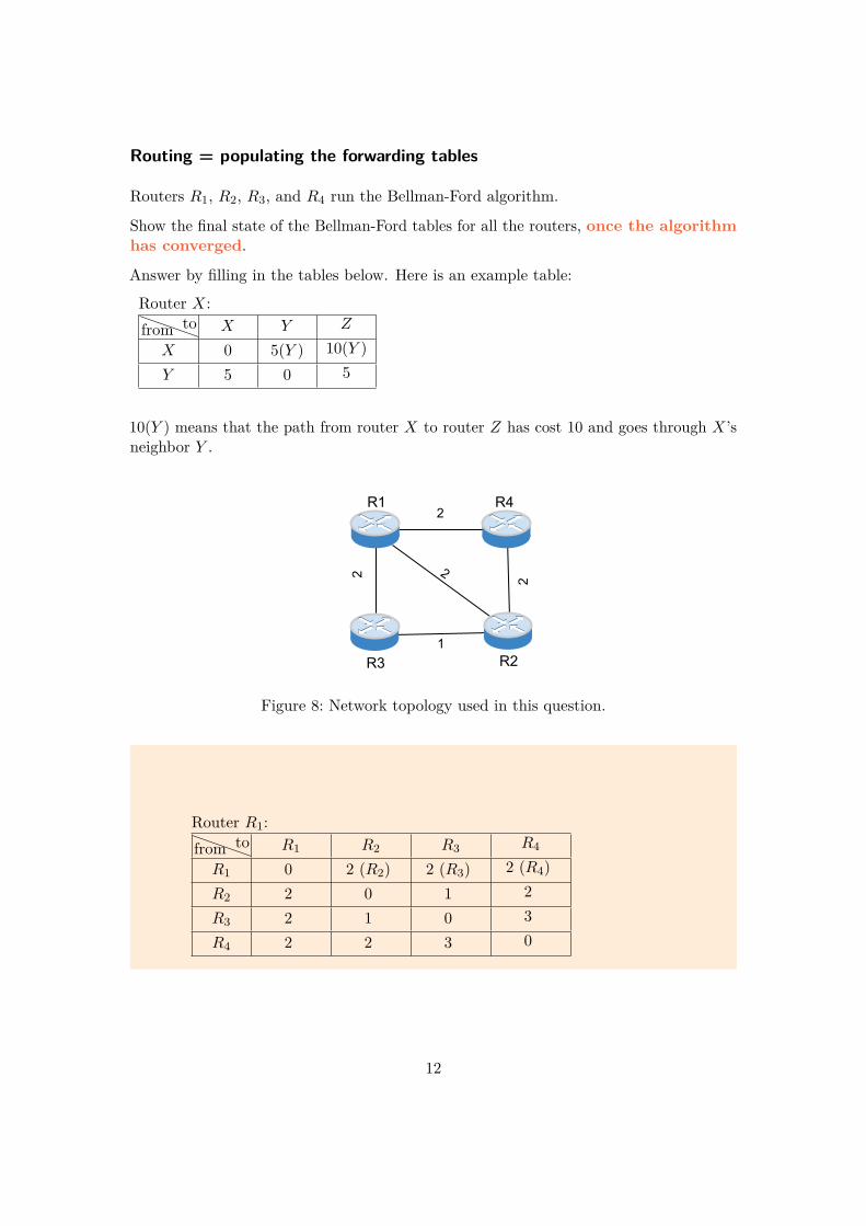
Routing = populating the forwarding tables

Routers R1, R2, R3, and R4 run the Bellman-Ford algorithm.

Show the final state of the Bellman-Ford tables for all the routers, once the algorithmhas converged.

Answer by filling in the tables below. Here is an example table:

Router X:from to X Y Z

X 0 5(Y ) 10(Y )Y 5 0 5

10(Y ) means that the path from router X to router Z has cost 10 and goes through X’sneighbor Y .

1

2

R3

R1

R2

R4 2

2

2

Figure 8: Network topology used in this question.

Router R1:from to R1 R2 R3 R4

R1 0 2 (R2) 2 (R3) 2 (R4)R2 2 0 1 2R3 2 1 0 3R4 2 2 3 0

12


R2 2 (R1) 0 1 (R3) 2 (R4)R1 0 2 2 2R3 2 1 0 ∞ (pr)R4 2 2 ∞ (pr) 0


R3 2 (R1) 1 (R2) 0 3 (R2)R1 0 2 2 2R2 2 0 1 2R4


R4 2 (R1) 2 (R2) 3 (R2) 0R1 0 2 2 2R2 2 0 1 2R3

13

Routing in the presence of link failures

The link between routers R1 and R2 fails.

Show the Bellman-Ford tables for all the routers from the moment the link fails anduntil the algorithm has re-converged. Write clearly after how many interactions(neighbor exchanges) the algorithm re-converges.

Answer by filling in the tables below. We have provided tables for two iterations, but thealgorithm may reconverge faster (in which case you just leave some tables empty).

1

2 R3

R1

R2

R4 2

2 ∞

Figure 9: Network topology after the link failure.

State after the link failure:


R1 0 3 (R3) 2 (R3) 2 (R4)R2

R3 2 1 0 3R4 2 2 3 0


R2 3 (R3) 0 1 (R3) 2 (R4)R1

R3 2 1 0 ∞ (pr)R4 2 2 ∞ (pr) 0

14

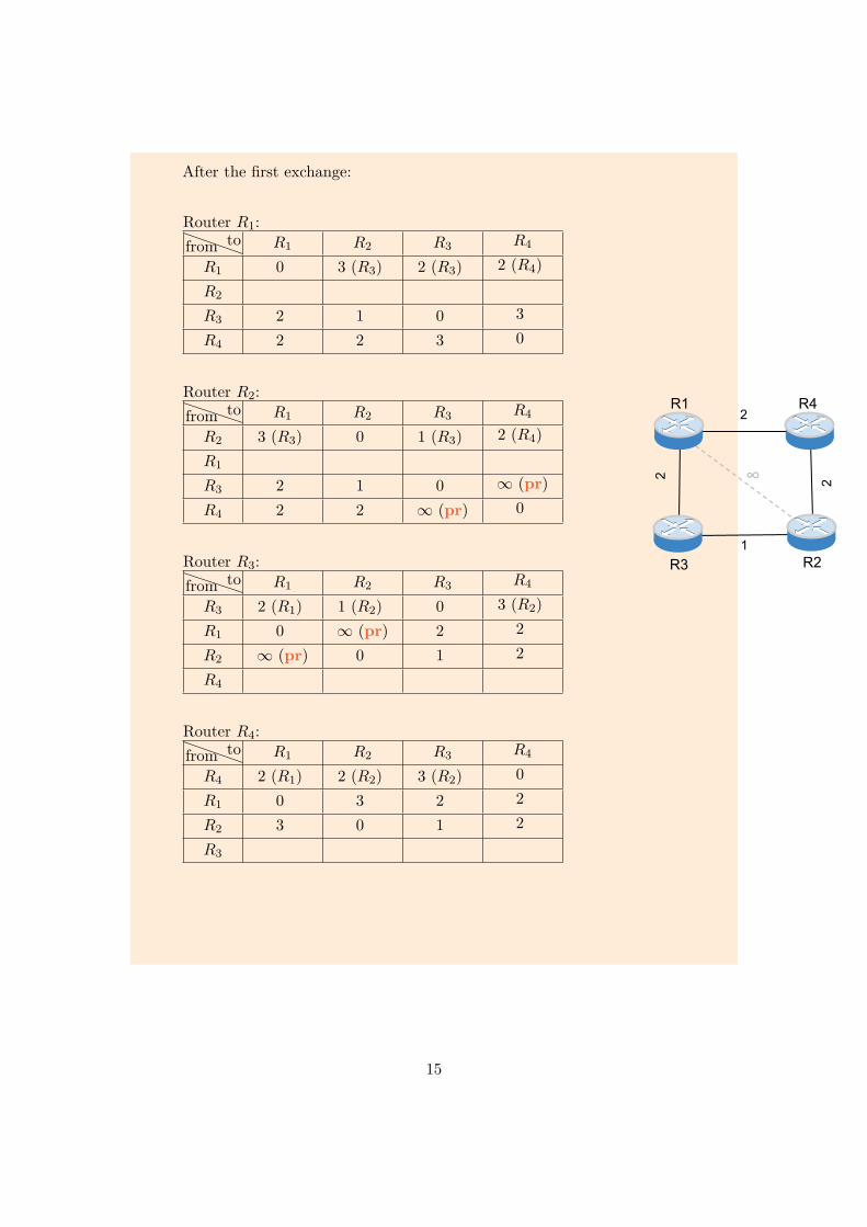
After the first exchange:


R1 0 3 (R3) 2 (R3) 2 (R4)R2

R3 2 1 0 3R4 2 2 3 0


R2 3 (R3) 0 1 (R3) 2 (R4)R1

R3 2 1 0 ∞ (pr)R4 2 2 ∞ (pr) 0


R3 2 (R1) 1 (R2) 0 3 (R2)R1 0 ∞ (pr) 2 2R2 ∞ (pr) 0 1 2R4


R4 2 (R1) 2 (R2) 3 (R2) 0R1 0 3 2 2R2 3 0 1 2R3

1

2

R3

R1

R2

R4 2

2 ∞

15

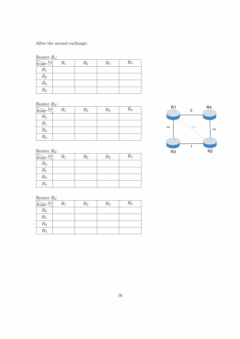
After the second exchange:


R1

R2

R3

R4


R2

R1

R3

R4


R3

R1

R2

R4


R4

R1

R2

R3

1

2

R3

R1

R2

R4 2

2 ∞

16

hw6: routing - solutions

Documents