DI

SC

US

SI

ON

P

AP

ER

S

ER

IE

S

Forschungsinstitut zur Zukunft der ArbeitInstitute for the Study of Labor

How Do Informal Agreements and RenegotiationShape Contractual Reference Points?

IZA DP No. 6095

October 2011

Ernst FehrOliver HartChristian Zehnder

How Do Informal Agreements and Renegotiation Shape Contractual

Reference Points?

Ernst Fehr University of Zurich

and IZA

Oliver Hart

Harvard University

Christian Zehnder

University of Lausanne

Discussion Paper No. 6095 October 2011

IZA

P.O. Box 7240 53072 Bonn

Germany

Phone: +49-228-3894-0 Fax: +49-228-3894-180

E-mail: iza@iza.org

Any opinions expressed here are those of the author(s) and not those of IZA. Research published in this series may include views on policy, but the institute itself takes no institutional policy positions. The Institute for the Study of Labor (IZA) in Bonn is a local and virtual international research center and a place of communication between science, politics and business. IZA is an independent nonprofit organization supported by Deutsche Post Foundation. The center is associated with the University of Bonn and offers a stimulating research environment through its international network, workshops and conferences, data service, project support, research visits and doctoral program. IZA engages in (i) original and internationally competitive research in all fields of labor economics, (ii) development of policy concepts, and (iii) dissemination of research results and concepts to the interested public. IZA Discussion Papers often represent preliminary work and are circulated to encourage discussion. Citation of such a paper should account for its provisional character. A revised version may be available directly from the author.

IZA Discussion Paper No. 6095 October 2011

ABSTRACT

How Do Informal Agreements and Renegotiation Shape Contractual Reference Points?*

Previous experimental work provides encouraging support for some of the central assumptions underlying Hart and Moore (2008)’s theory of contractual reference points. However, existing studies ignore realistic aspects of trading relationships such as informal agreements and ex post renegotiation. We investigate the relevance of these features experimentally. Our evidence indicates that the central behavioral mechanism underlying the concept of contractual reference points is robust to the presence of informal agreements and ex post renegotiation. However, our data also reveal new behavioral features that suggest refinements of the theory. In particular, we find that the availability of informal agreements and ex post renegotiation changes how trading parties evaluate ex post outcomes. Interestingly, the availability of these additional options affects ex post evaluations even in situations in which the parties do not use them. JEL Classification: C91, D03, D86, J41 Keywords: contracts, reference points, fairness, renegotiation, informal agreement Corresponding author: Ernst Fehr Department of Economics University of Zurich Blümlisalpstrasse 10 8006 Zürich E-mail: ernst.fehr@econ.uzh.ch

* We gratefully acknowledge financial support from the U.S. National Science Foundation through the National Bureau for Economic Research and the Research Priority Program of the University of Zurich on the “Foundations of Human Social Behavior”. We would like to thank Heski Bar-Isaac, Roland Benabou, Sylvain Chassang, Bob Gibbons, Wolfgang Pesendorfer, and Philipp Weinschenk for helpful comments.

1

I. Introduction

A series of recent theory papers develops the idea that ex ante contracts may serve as

reference points for ex post trade (see Hart and Moore 2008, Hart 2009, Hart and Holmström

2010). The theoretical work not only helps us to understand the role of long-term contracts in

the absence of non-contractible investments, but also sheds light on the internal organization

of the firm, and provides a new perspective on authority and delegation. However, the theory

rests on strong behavioral assumptions that deviate from standard contract theory. While

initial tests provide encouraging support for the new approach (see Fehr, Hart, and Zehnder

2009, 2011), these experiments also have limitations. Most important, the experimental setups

ignore real-life aspects of trading relationships such as informal agreements and renegotiation.

As there are plausible reasons for these features to be important, we carry out new

experiments to investigate their relevance. Our evidence suggests that the central behavioral

mechanism underlying the concept of contractual reference points is robust to the possibility

of informal agreements and renegotiation, although new behavioral features emerge.

To clarify our contribution and embed it in the existing literature, it is helpful to start

with some background and motivation. While standard incomplete contract models (see

Grossman and Hart 1986 and Hart and Moore 1990) are useful for studying the determinants

of asset ownership and the boundaries of firms, they do not help much for understanding the

internal organization of larger firms. The reason is that these models are based on the

assumption that Coasian bargaining ensures ex post efficiency, so that it is hard to see why the

internal structure of firms should matter. To move towards more general and compelling

theories of contracts and organizational form, Hart and Moore (2008) depart from the existing

literature and drop the assumption that ex post trade is perfectly contractible. In addition, they

introduce the behavioral concept that ex ante contracts, negotiated under (relatively)

competitive conditions, shape parties’ entitlements regarding ex post trade. If a party does not

get what he feels entitled to he is aggrieved and provides perfunctory rather than consummate

performance, causing deadweight losses. These new assumptions deliver a trade-off between

rigid and flexible contracts and have significant organizational implications: among other

things, they can explain employment contracts, which fix wages in advance and leave

discretion to the employer over the task. Hart (2009) reintroduces asset ownership and shows

that the presence of contractual reference points can explain the use of indexation in contracts

and the role of payoff uncertainty in determining vertical integration. Hart and Holmström

(2010) apply the idea of contractual reference points to firm scope, authority and delegation.

2

While these results are promising, they are convincing only if the strong behavioral

assumptions on which they rely are empirically valid. Fehr et al. (2011, henceforth FHZ)

provide initial tests of the Hart-Moore theory. They set up a controlled laboratory experiment

based on the payoff uncertainty model in Hart and Moore (2008). In line with the prediction

of the model the experiments show that there is an important trade-off between contractual

rigidity and flexibility. Flexible contracts are useful because they allow the trading parties to

adjust the terms of the contract to the realized state of the world. However, flexibility causes

significant shading in ex post performance as parties seem to have misaligned reference

points. Contractual rigidity is helpful to overcome the shading problem, because a

competitively determined fixed price aligns ex ante expectations and avoids ex post

aggrievement. But rigid contracts suffer from the problem that their fixed terms prevent

mutually beneficial exchanges from occurring in some states of the world. These results are

reassuring for the theory, given that the different implications of rigid and flexible contracts

for ex post performance are the basis for most organizational implications derived from the

models.2 It is also noteworthy that the behavior observed in these experiments cannot be

explained either by traditional contract theory or by standard behavioral models.3

However, while the experimental results reported in FHZ are supportive of the theory

of contractual reference points, there are some limitations. Two important caveats are that the

experimental setup does not allow either for informal agreements or for ex post renegotiation.

Both these features are relevant in many real-life trading relationships and there are plausible

reasons why each of them might change how ex ante contracts affect ex post behavior.

To understand why informal agreements may matter, note that the Hart-Moore model

assumes that states of the world are ex post observable but not verifiable. This assumption is

standard in the incomplete contracts literature and implies that the parties cannot rely (at least

directly) on state-contingent contracts. However, ex post observability suggests that the

trading parties could reach informal, state-contingent agreements. The standard economic

approach deems such informal agreements irrelevant cheap-talk. However, if contracts

constitute reference points they may matter. Contractual reference points imply that ex post

performance depends on ex ante expectations. If the parties can use informal agreements to

2 Erlei and Reinhold (2011) replicate the experiment of FHZ. Although they find higher shading levels in both types of contracts, they confirm the existence of the trade-off between contractual rigidity and flexibility. 3 In particular, existing theories of social preferences (Fehr and Schmidt 1999, Bolton and Axel Ockenfels 2000, Rabin 1993, Charness and Rabin 2002, Dufwenberg and Kirchsteiger 2004, Falk and Fischbacher 2006) cannot account for the observed trade-off between rigid and flexible contracts. See FHZ.

3

“manage” expectations, these agreements may have important consequences. Instead of

relying on rigid contracts, the trading parties could align reference points by combining

flexible contracts with informal agreements. Such enhanced flexible contracts would be

attractive as they would not only guarantee trade, but would also avoid inefficiencies caused

by aggrievement and shading. In this sense the presence of informal agreements might destroy

the trade-off between rigidity and flexibility. Hart and Moore (2008) abstract from informal

agreements, arguing that subjective interpretations of states and self-serving biases make it

unlikely that such agreements shape reference points. However, ultimately the role of

informal agreements remains an empirical question.

To see why ex post renegotiation might be important, suppose that a buyer and a seller

have agreed on a rigid ex ante contract. Ex post it turns out that the seller’s costs are higher

than the fixed price. Without renegotiation voluntary trade implies that the seller walks away

and realizes an outside option. In reality, however, it is unclear whether this is plausible. As

long as the buyer’s value is higher than the seller’s cost, what would prevent the parties from

renegotiating their contract and enjoying the gains from trade? Thus, the availability of

renegotiation would also seem to cast doubt on the trade-off between rigid and flexible

contracts: rigid contracts may achieve the best of both worlds by aligning expectations and

avoiding ex post inefficiency.

However, renegotiation raises a number of potential issues. First, even in the situation

described above it is not clear how profitable trade is after renegotiation. Although the

renegotiation is mutually beneficial, it reintroduces flexibility regarding the price choice and

may lead to misaligned expectations, aggrievement and shading. Second, renegotiation may

complicate situations in which trade would be feasible under the initial contract. A first

possibility is opportunistic renegotiation: a party may initiate renegotiation just to grab a

bigger share of the surplus. This may create bad feelings, shading, and significant

inefficiency. Another problem is that rigid contracts may no longer align reference points in

the first place. If renegotiation is always feasible, people may start to hope for outcomes

outside the contract. In this case performance may suffer from shading even if the parties

carry out the initially agreed upon contract.

In this paper we design new experiments that throw light on both informal agreements

and renegotiation. Our first experiment reveals that, although informal agreements have an

impact, they do not eliminate the trade-off between contractual rigidity and flexibility. If

buyers explicitly (by announcing low prices) or implicitly (by not making an announcement)

4

indicate that they are not willing to pay a high price, sellers are less aggrieved and less likely

to engage in shading in response to a low final price than in the baseline treatment where price

announcements are not feasible. However, shading is considerably higher if buyers choose

lower prices ex post than they announced ex ante. Thus buyers who attach an informal

message to a flexible contract are best off if they announce a low price and stick to it.

Somewhat surprisingly, we find that not making a price announcement at all is as good as

making a low price announcement. It seems that a flexible contract without a message is

evaluated differently by sellers depending on whether informal agreements are feasible or not:

sellers tend to interpret the lack of an explicit price announcement as an implicit message that

the buyer has no intention to pay a high price.

The overall lower shading in flexible contracts increases their attractiveness for buyers

relative to the baseline condition. However, the decrease in shading rates is only moderate and

not sufficient to eliminate the trade-off between contractual rigidity and flexibility. Even

when informal agreements are available, it is still true that lower prices trigger more shading

in flexible contracts than in rigid ones. As a result, buyers who choose rigid contracts realize

higher profits in the good state of the world than if they choose flexible contracts. This

advantage of rigid contracts is large enough to offset the disadvantage that rigid contracts do

not allow for trade in the bad state. The consequence is that on average flexible contracts are

no more profitable than rigid contracts.

We think that the finding that informal agreements do not eliminate the trade-off

between rigidity and flexibility is important, especially because the simplicity of our setup

(only two possible states, completely symmetric information) gives informal agreements a

very good chance to be effective. The effects of informal agreements are likely to be smaller

in more complicated situations.

Our findings contribute to the literature on pre-play communication. While it has been

well established that pre-play communication fosters cooperation (see, e.g., Sally 1995,

Ledyard 1995) and coordination (see, e.g., Crawford 1998), our data points out a very

different aspect: if market participants decide not to make use of available ex ante

communication opportunities, their ex post actions are evaluated differently than in a situation

in which communication has not been feasible. This resonates with earlier evidence indicating

that variations in the set of available but not chosen alternatives can importantly change how a

trading partner perceives a specific action (see e.g., Charness and Rabin 2002, Falk et al.

5

2003). Our findings suggest that these effects may apply not only to variations in the payoff-

relevant action space, but also to modifications of non-binding communication opportunities.

Our second experiment investigates the effects of ex post renegotiation. We implement

a rather extreme form of renegotiation. We allow the buyer unilaterally to replace the existing

contract with a new one: since the seller has no veto, this is actually closer to what lawyers

call a “repudiation”. We consciously chose this particular form of renegotiation, because the

fact that contracts can be abandoned at no cost gives renegotiation the best chance to

minimize the behavioral impact of contracts. In this sense our treatment is a powerful stress

test for the relevance of contractual reference points. We find that renegotiation opportunities

do not imply that contractual reference points are irrelevant. Although renegotiation is always

feasible, the trading parties do not seem to hope for outcomes outside the contract when trade

is feasible within the contract. Specifically, if the buyer in a rigid contract decides to stick to

the agreed upon price in the good state, the shading rate remains the same as in the baseline

treatment. Sellers still seem to accept the competitively negotiated fixed price as a reference

point and do not feel entitled to an upward renegotiation of the price as long as the price

allows for trade. This is a strong finding. As the buyer can unilaterally change the contract in

this treatment, the contract choice is ultimately a framing decision without consequences for

feasible outcomes. Nevertheless, we find that contracts serve as salient reference points. This

makes it likely that contractual reference points also remain important in more realistic

situations, where renegotiation may be more difficult and/or costly.

In addition, we find that the possibility of renegotiation increases the attractiveness of

rigid contracts in the bad state. In this situation renegotiation allows the buyers to transform a

rigid contract into a flexible one that permits them to increase the price to cover the seller’s

cost. While these mutually beneficial renegotiations of a rigid contract trigger some shading

activities on the seller side (probably as a consequence of the misaligned entitlements caused

by the newly introduced flexibility), the gains from trade are still substantial. Thus, overall,

buyers who choose rigid contracts manage to realize significantly higher profits in the

presence of renegotiation opportunities than in their absence.

However, renegotiation is problematic to the extent that buyers behave

opportunistically, i.e., they breach the contract to lower the price and grab a larger share of the

surplus. In this case most of the affected sellers seem to be aggrieved and there is a large and

significant increase in shading. It seems that most buyers anticipate the sellers’ reaction and

therefore opportunistic renegotiation occurs almost exclusively in the rare situations where the

6

competitive ex ante process yielded unfavorable terms for the buyer. Our finding that

opportunistic renegotiation triggers inefficient shading has important implications for the

hold-up literature. While the leading formal models ignore the possibility that renegotiation

may trigger counterproductive reactions (see, e.g., Grossman and Hart 1986 and Hart and

Moore 1990), recent theoretical work suggests that taking into account the psychological

aspects of renegotiation may have important implications. In particular, Hart (2009) shows

that such a behavioral model allows us to identify payoff uncertainty as a driving force of

organizational form, a result which resonates well with empirical findings on vertical

integration (see Lafontaine and Slade 2007, for a review).

Interestingly, and perhaps surprisingly, the availability of renegotiation also seems to

have an impact on sellers’ evaluations of outcomes in flexible contracts. While higher shading

rates still imply that buyers’ profits are significantly lower in non-renegotiated flexible

contracts than in non-renegotiated rigid contracts in the good state, this difference is

significantly smaller in the renegotiation treatment than in the baseline condition.

Renegotiation opportunities seem to render the choice of inequitable terms in non-

renegotiated contracts more acceptable, i.e., as long as the buyer adheres to the contract,

sellers are less likely to engage in shading when the buyer picks a low price as compared to

the baseline condition. While this behavior may be partly attributable to our assumption that

buyers can unilaterally change the contract (i.e., no veto for sellers), it also reinforces the view

that available but not chosen alternatives shape perceptions. The lower shading rates also

imply that flexible contracts are more attractive for buyers when renegotiation is available.

However, if buyers renegotiate optimally (i.e., no opportunistic renegotiations), rigid contracts

still yield higher overall profits for buyers than flexible contracts.

To summarize, both our experiments provide further evidence that contractual

reference points shape performance in relationships governed by incomplete contracts. In

addition, our evidence suggests interesting refinements regarding the theory. We find that the

trading parties’ evaluation of the ex post outcome is influenced by informal agreements and

ex post renegotiation and that the availability of these additional options affects ex post

evaluations even in situation in which the parties do not use them.

The remainder of the paper is organized as follows: In Section II, we describe the

design of our experiment and provide details of procedures. Section III contains the

behavioral predictions. We present and discuss our results in Section IV. Section V concludes.

7

II. Experimental Design

We present the market setup and the parameters in Section II.A. Section II.B describes the

interaction of buyers and sellers in the experiment. The details of the different experimental

conditions that we investigate are provided in Section II.C. We describe the laboratory

procedures in Section II.D.

II.A. Market Setup and Parameters

Each experimental session has an equal number of buyers and sellers. In every period of the

experiment buyers and sellers have the possibility to trade a product. Since each seller can sell

up to two units, but every buyer can buy at most one unit of the product per period, the supply

of the product is twice as large as the demand. Thus, sellers face competition for buyers.

When a buyer purchases a unit of the product from a seller, his payoff is equal to his valuation

for the product v minus the price p. The payoff of the seller is defined as the difference

between the price p and the production cost c. The buyer’s valuation for the product depends

only on the seller’s ex post quality choice q. The seller’s production cost, in contrast, also

depends on the realized state of the world . There are two states of nature: a good state ( =

g), in which the seller’s production costs are low, and a bad state ( = b), in which the

production costs are high. The good state occurs with probability wg = 0.8.

The payoffs of buyers and sellers can be summarized as follows:

Buyer’s payoff: B = v(q) – p.

Seller’s payoff: S = p – c(q, ).

When trade occurs sellers can choose between two quality levels: normal quality (q = qn) or

low quality (q = ql). The production costs for low quality are slightly higher than the

production costs for normal quality: c(ql, ) > c(qn, ). This reflects the idea that sellers can

minimize costs if they simply provide the product desired by the buyer. However, they can

sabotage output (at a small cost) if they want to.4 For each unit of the product which a seller

cannot sell – either because he did not manage to conclude a contract with a buyer or because

4 The quality choice of the seller in our experiment is similar to costly punishment technologies that have been used in many other cooperation experiments (see, e.g., Fehr and Gaechter (2000) for a typical example). However, it is important to notice that our experiment differs from the typical gift exchange experiments (see, e.g., Fehr et al. (2009) for a review of this literature). In gift-exchange games the pecuniary incentive for workers (i.e., sellers) is to provide the minimal effort (i.e., quality) level, whereas in our paper the normal quality level maximizes seller earnings.

8

his contract does not allow for a mutually beneficial trade – he realizes an outside option xS =

10. When a buyer is unable to trade, he also realizes an outside option xB = 10. Table 1

summarizes the cost and value parameters of the experiment:

In the experiment sellers and buyers interact in groups of four (two buyers and two sellers).

To minimize the role of reputational considerations, these groups are randomly reconstituted

at the beginning of every period. Thus, our protocol induces a series of one-shot interactions.

II.B. Interaction of Buyers and Sellers Within a Period of the Experiment

In the following we describe the different steps which characterize the interaction of buyers

and sellers in all our treatments. Particularities of the different experimental condition are

discussed in the next section:

Random formation of interaction groups:

At the beginning of every period a computerized random device defines the interaction

groups consisting of two buyers and two sellers.

Phase 1: Ex ante contracting:

Step 1: Buyers’ contract choice

Each transaction begins with the buyer’s choice of a contract type (t). The buyer has to

decide whether he wants to offer a rigid contract (t = r) or a flexible contract (t = f). Rigid

contracts already define a fixed transaction price pr ex ante. Flexible contracts, in contrast,

specify only a price range [pl, pu] from which the price can be chosen ex post. It is

important to note that the buyer can choose only the type of contract, but not the terms.

The terms (i.e., the fixed price or the price range, respectively) are determined in a

competitive auction among the sellers.

Step 2: Sellers’ contract auction

After both buyers in an interaction group have chosen their type of contract, the two

contracts are auctioned off to the sellers. The sequence of the auctions is randomly

determined within each group. If a rigid contract is auctioned off the auction directly

determines the fixed price pr [c(ql,g) + xS, 75] = [35, 75].5 In a flexible contract the

5 The minimum of 35 for the fixed price ensures that the seller cannot make losses relative to his outside option in the good state even if he provides low quality. This feature guarantees that sellers do not refrain from

9

auction determines the lower bound of the price range pl [35, 75]. The upper bound of

the price range is exogenously fixed and equal to the buyer’s valuation of the product

when the seller provides normal quality: pu = v(qh) = 140. Thus, in both cases the auction

starts off at 35 and then increases by one unit every half second. Each of the two sellers

has a button that allows him to accept the contract at any time during the auction. Thus,

the first seller who is willing to accept the displayed fixed price or the displayed lower

bound respectively gets the contract. The seller who loses the auction and does not get the

contract directly realizes the outside option xS.

Determination of the state of the world:

After the contract auctions the computer randomly determines the state of the world for

each contract independently. The state is common knowledge to the trading parties.

Phase 2: Ex post trading:

Step 3: Buyers’ choice of contract terms

Once the state has been revealed, the buyer determines the final terms of the contract.

How much flexibility he has in doing this depends on the experimental condition and the

ex ante chosen contract. To initiate a mutually beneficial trade the buyer needs to be able

to pick a price that covers the seller’s cost. The flexible contract always allows for such a

choice, but the fixed price contract does not: in the bad state the fixed price of a rigid

contract is lower than the seller’s cost (pr [c(ql,g) + xS, 75] < c(qn,g) = 80 < c(ql,g) = 85).

In the latter case trade is feasible only if the buyer can renegotiate the contract

(renegotiation is permitted in only one of our experimental conditions). If the buyer

cannot or does not want to renegotiate the contract, trade does not occur and both trading

parties realize their outside options. If the contract allows for trade the buyer either pays

the fixed price (rigid contract) or picks a price out of the available price range (flexible

contract, or if a contract has been renegotiated).6

choosing low quality, just because they want to avoid losses (loss aversion). The maximum of 75 for the fixed price ensures that the price is always below the seller’s cost in the bad state of the world. This guarantees that trade is infeasible within rigid contracts if the bad state is realized. However, in the experiment the competitive forces in the auction were strong enough so that the maximum was never binding. 6 In the bad state the buyer has to ensure that the price is such that the seller cannot make losses, i.e., he must choose a price p [c(ql,b) + xS, v(qh)] = [95, 140]. Again we do not allow prices to be such that the seller can make losses by choosing low quality, since we want to avoid the possibility that people refrain from shading because of loss aversion (see also Footnote 5).

10

Step 4: The seller’s quality choice

Sellers observe the price choice of their buyer and then determine their quality. The sellers

always have the choice between normal (qn) and low (ql) quality. Remember that choosing

low instead of normal quality increases the seller’s cost by 5 units irrespective of the

contract type and realized state of the world (see Table 1).

Payoffs and Market Information:

When all decisions have been made, profits are calculated and displayed on subjects’

screens. In addition, to their profit information buyers also get some aggregated

information about the market outcome.7

Subsequently. a new period begins and the participants are randomly reassigned to a new

interaction group.

II.C. Experimental Treatments

In the following we describe our two main treatment conditions. For completeness we also

provide the details of the baseline condition of FHZ, because we later use this condition as a

benchmark for our results.

The Informal Agreement Condition (IA):

In the informal agreement condition buyers who choose a flexible contract in Step 1 can

decide whether they want to combine the contract with a message of the following form:

“If costs are low, I plan to pay a price of pA(g). If costs are high, I plan to pay a price

of pA(b).”

The price announcements are in no way binding for the buyer, i.e., the message does not

affect the range of actual prices available to the buyer ex post. The buyer can always pick

prices which are higher or lower than the announced price if the competitively determined

price range of the contract allows for this. All market participants are informed about the

presence of the message opportunity in flexible contracts in the instructions of the experiment,

i.e., the availability of messages is common knowledge in the experiment.

7 The buyers are informed about average payoffs in rigid and flexible contracts of all buyers in all previous periods. In addition, they also learn how many buyers have chosen rigid and flexible contracts in the current period. The aim of the provision of this information is to make learning easier for buyers. Since our setup allows for many possible constellations (two contract types, two states of nature, two quality levels, many prices), learning from individual experience is rather difficult.

11

In the informal agreement condition renegotiation of contracts is not permitted.

Accordingly, rigid contracts allow for trade only if the good state of the world is realized. In

the bad state trading parties with a rigid contract have to realize their outside option.

The Renegotiation Condition (RG):

In the renegotiation condition, there are no informal agreements. However, buyers always

have the possibility to renegotiate the contract ex post (see Step 3 above). If a buyer decides

to renegotiate the contract, the original contract is no longer of relevance and the buyer can

choose any price that satisfies p [c(ql, ) + xs, 140]. The seller cannot veto the buyer’s

decision to renegotiate the terms.8 Renegotiation is available for rigid and flexible contracts in

both states of the world, i.e., the buyer can always decide whether he wants to stick to the

competitively concluded ex ante contract and accept the imposed restrictions (i.e., the fixed

price in rigid contracts and the lower bound of the price range in flexible contracts,

respectively) or whether he wants to abandon the contract and pick his price without

restrictions.

It is useful to distinguish three types of renegotiation which may occur in this

condition. First, the buyer may renegotiate a rigid contract in the bad state of the world. This

allows for a price increase and makes trade feasible. As both parties benefit (at least weakly)

from such a renegotiation, we call this a “mutually beneficial renegotiation”. Second, the

buyer may renegotiate a contract in the good state of the world in order to decrease the price

to a level below the ex ante agreed upon fixed price or lower bound of the price range,

respectively. We call this an “opportunistic renegotiation”, because the buyer intends to

increase his own profit at the expense of the seller. Finally, there is also the possibility that a

buyer voluntarily increases the fixed price of a rigid contract in the good state of the world.

As this is a costly attempt to increase the seller’s profit we call this an “altruistic

renegotiation”.

The Baseline Condition of FHZ (BL)

In the baseline condition of FHZ neither informal agreements nor ex post renegotiation are

available.

8 We discuss this feature of the experiment in detail in section III.C.

12

II.D. Subjects, Payments and Procedures

All subjects were students of the University of Zurich or the Swiss Federal Institute of

Technology Zurich (ETH). Economists and psychologists were excluded from the subject

pool. We used the recruitment system ORSEE (Greiner 2004). Each subject participated in

only one session. Subjects were randomly subdivided into two groups before the start of the

experiment; some were assigned the role of buyers and others the role of sellers. The subjects’

roles remained fixed for the whole session. All interactions were anonymous, i.e., the subjects

did not know the personal identities of their trading partners.

To make sure that subjects fully understood the procedures and the payoff

consequences of the available actions, each subject had to read a detailed set of instructions

before the session started. Participants then had to answer several questions about the feasible

actions and the payoff consequences of different actions. We started a session only after all

subjects had correctly answered all questions. The exchange rate between experimental

currency units (“points”) and real money was 15 Points = 1 Swiss Franc (~US $ 1, in

November and December 2010).

In order to make the sellers familiar with the auction procedure we implemented two

trial auctions – one with a rigid contract and one with a flexible contract – before we started

the actual experiment. In the trial phase each seller had his own auction, i.e., they did not

compete with another seller and no money could be earned.

The experiment was programmed and conducted with z-Tree (Fischbacher 2007). We

conducted 5 sessions of the informal agreement condition, and 5 sessions of the renegotiation

condition. We had 28 subjects (14 buyers and 14 sellers) in 5 of our 10 sessions and – owing

to no-shows – 24 subjects (12 buyers and 12 sellers) in 4 sessions, and 20 subjects (10 buyers

and 10 sellers) in 1 session. This yields a total number of 256 participants in the experiment.

A session lasted approximately two hours and subjects earned on average about 50 Swiss

Francs (including a show-up fee of 10 Swiss Francs).

III. Behavioral Predictions

In this section we derive a set of hypotheses for our experiment. In section III.A we present

the predictions that result from the assumption that people are purely self-interested money-

maximizers. While we do not believe that the self-interest hypothesis is an accurate

description of our participants’ behavior, we still feel that these predictions are a useful

13

benchmark, not least because much of the theoretical literature on incomplete contracts is

based on models that assume pure self-interest. In section III.B we discuss how the presence

of contractual reference points affects the predictions for our experiment. As there are always

different ways to design a particular experiment we use section III.C to discuss some features

of our design and their role for the interpretation of the results.

III.A. Predictions under Pure Self-Interest

The prediction of the self-interest model is straightforward. Buyers anticipate that selfish

sellers are never willing to engage in costly shading and therefore offer the lowest price

permitted by the contract. Competition in the contract auctions implies that the fixed price in

rigid contracts and the lower bound in flexible contracts are at the competitive level, i.e. pr =

35 and pl = 35.9 This implies that rigid and flexible contracts yield the same profit for buyers

in the good state of the world (B = v(qn) – p = 140 – 35 = 105). In the bad state payoffs

depend on whether renegotiation is available. If the buyer can renegotiate the contract, both

contracts yield the same profit for the buyer (B = v(qn) – p = 140 – 95 = 45) and the buyer is

indifferent between the two. If renegotiation is not possible, the rigid contract results in the

outside option (B = xB = 10) and therefore the buyer strictly prefers the flexible contract.

Whether or not informal agreements are available does not affect the predictions.

We summarize the prediction of the standard economic model as the

Standard Hypothesis:

a) Market forces imply that the fixed price in rigid contracts and the lower bound of the

price range in flexible contracts end up at the competitive level, i.e., pr = pl =35.

b) Sellers never choose low quality irrespective of the contract type and price level.

Buyers always choose the lowest price available in flexible contracts.

c) In the absence of renegotiation opportunities buyers’ profits are higher in flexible

contracts than in rigid contracts. Therefore, buyers prefer flexible contracts.

d) The presence of informal agreements does not affect outcomes.

9 Remember: Since p = 35 corresponds to p = c(ql,g) + xS and the seller must offer at least p = c(ql,b) + xS = 95 in the bad state of the world, a seller can never be worse off if he accepts a contract than if he accepts his outside option.

14

e) When ex post renegotiation is possible, both types of contracts yield identical payoffs

and buyers are indifferent between them (if they choose the rigid contract, they always

renegotiate the price from pr = 35 to p = 95 if the bad state is realized).

III.B. Predictions if Contracts are Reference Points

In this section we discuss how the Hart-Moore notion that competitively negotiated ex ante

contracts provide reference points for ex post trade affects the predictions for each of our

experimental conditions. In FHZ we provide a slightly modified version of the Hart-Moore

model and derive the following prediction for the baseline treatment: While contractual

reference points do not affect the prediction that the contract auctions yield competitive

outcomes (pr = pl =35), they change the consequences of the buyers’ contract choice. Of

particular importance is the fact that flexible contracts may induce sellers to hope for high

prices.10 If a buyer picks a price which is below the seller’s reference price, the seller may be

aggrieved and engage in shading. As sellers may have heterogeneous reference points the

frequency of shading is predicted to be decreasing in price. Thus, depending on the

distribution of sellers’ reference prices it can be optimal for the buyer either to increase the

price to avoid shading or to accept the risk of getting low quality. Rigid contracts should

avoid the shading problem, because they pin down the price from the outset and thereby fix

expectations. Thus, if the shading problem in flexible contracts is severe enough, rigid

contracts may be more profitable for buyers, even though they prevent the parties from

trading in the bad state of the world.

Next we discuss the predictions for our new experimental conditions in the light of

contractual reference points. We begin with the informal agreements condition. In FHZ we

assume that the reference price is a function of the type of contract (t) and the state (): pR(t,

). A rigid contract allows for only one price so that the reference price is equal to the fixed

price: pR(r, ) = pr. In flexible contracts we assume that the reference price can be any price

permitted by the contract (i.e., we allow for heterogeneity in sellers’ reference points): pR(f, )

10 Hart and Moore (2008) assume that each party compares the ex post outcome to the most favorable outcome permitted by the contract. In FHZ we extend the model to allow for the case where parties may have heterogeneous reference points, i.e., we take into account that some traders may feel entitled to an outcome other than the most favorable outcome. We show that the predictions of such an extended model remain very similar to those of the original model.

15

[pl, pu]. The role of the reference point for the seller’s utility is illustrated by the following

equation:

uS = S – max[(pR(t, ) – p), 0] I(q),

where 0 and I(q) is an indicator function, which is unity if q = qn and zero otherwise. The

second term captures the psychic costs of aggrievement, which become relevant if the realized

price p is smaller than the seller’s reference price pR. The parameter measures the intensity

of the seller’s aggrievement if he feels shortchanged. The indicator function I(q) captures the

idea that a seller can completely offset his aggrievement if he shades on performance and

thereby hurts the buyer by lowering his valuation for the delivered product. This formulation

implies that a seller engages in shading if the price is below the threshold price defined as:

pT() = pR(f, ) – [c(ql, ) – c(qn, ) / ].

We can now take up the idea that the trading parties may have the possibility to “manage” the

reference point in flexible contracts using informal agreements. To this end let pA() be an

informal (i.e., non-enforceable), state-contingent price announcement of the buyer. In our

experiment the price announcement is either a set of two prices (pA() = {pA(g), pA(b)}) or the

empty set (pA() = ). In accordance with the idea of managing expectations, we define the

reference price in a flexible contract when informal agreements are available as follows:

pR(f, , pA()) = pA() + (1 – ) pR(f, , ), where [0, 1].

This means we assume that the seller’s reference price in the presence of informal agreements

is a weighted average of the buyer’s price announcement pA() and the seller’s reference price

that he would have had in the absence of a price announcement. The weighting parameter

determines the importance of the price announcement for the reference price. If is equal to

one, this means that the buyer can fully control the seller’s reference point by informally

announcing a state-contingent price. If is equal to zero, this means that the buyer’s price

announcement is completely irrelevant, i.e., the seller feels entitled to the same price as in the

absence of a price announcement.

If is strictly positive, low price announcements reduce the reference price and

thereby the threshold price that ensures high quality (pR(f, )/ pA() = pT()/ pA() < 0).

We would therefore expect that buyers try to manage their seller’s reference points by

announcing low prices. Specifically, profit-maximization implies that buyers who choose a

16

flexible contract should combine the contract with a price announcement that informs the

seller that the buyer always plans to pay the lowest price possible:

pA() = {pA(g) = c(ql,g) + xs = 35, pA(b) = c(ql,b) + xS = 95}.

Such a price announcement shifts the distribution of sellers’ threshold prices to the left and

therewith maximizes the profitability of flexible contracts. If is equal to one, the optimal

price announcement above would allow the buyer to pay the competitive price while

completely avoiding shading in flexible contracts. If this is the case, the availability of

informal agreements would imply that buyers would strictly prefer the flexible contract,

because a flexible contract would not only generate the same profit as a rigid one in the good

state, but it would also make (shading-free) trade feasible in the bad state. However, if is

sufficiently small, the positive impact of low price announcements on the profitability of

flexible contracts may be small and rigid contracts may remain more attractive than flexible

ones.

We now turn to the role of renegotiation in our setup. Let {–1, 0, 1} be the buyer’s

renegotiation decision, where equal to zero signifies the absence of renegotiation, equal to

minus one stands for opportunistic renegotiation, and equal to one captures mutually

beneficial or altruistic renegotiation. The availability of renegotiation raises two important

questions regarding contractual reference points. The first one is: do contracts remain

reference points even when renegotiation is always feasible? And the second question is: how

is the reference point determined once renegotiation has been initiated?

We first consider the question of whether contracts remain reference points in the

presence of renegotiation. This question is of great interest for the cases where the parties

decide to stick to the ex ante agreed upon contract, i.e., it is important to determine the seller’s

reference point if the buyer decides not to renegotiate the contract. Basically, there are two

interesting possibilities. One possibility is that the parties continue to hope for their preferred

outcome within the limits of the contract, i.e., the contract remains the reference point even

though renegotiation would have been possible. In this case the definition of reference prices

is not affected by the presence of renegotiation opportunities: pR(r, , = 0) = pR(r, ) = pr

and pR(f, , = 0) = pR(f, ) [pl, pu]. The argument for this possibility would be that sellers

explicitly agree to the contract in the competitive bargaining process and therefore it is not

unreasonable to assume that the contract is a focal point and defines their expectations.

17

The alternative view would be that contracts completely lose their meaning in the

presence of renegotiation opportunities and parties simply hope for their preferred outcome

within the set of all feasible outcomes (including ones that can be reached only if the contract

is renegotiated). This would actually imply that the reference prices are independent of both

the contract type and the renegotiation decision: pR() [c(ql,g) + xs, v(qn)]. As a

consequence, the buyer’s contract choice would no longer make any difference for ex post

performance. Which of these two views is realistic can be determined only by the data.

We now turn to the definition of the reference point after renegotiation. It is obvious

that this question is important only if contracts continue to shape reference points when

renegotiation is not initiated (otherwise the parties just hope for their preferred outcome

pR(); see above). One possible view is that renegotiation simply turns the existing contract

(be it a flexible or a rigid contract) into a completely flexible contract with price range p

[c(ql,g) + xs, v(qn)]. Accordingly, the reference point after renegotiation would be pR(t, , ≠

0) = pR(f, ) [c(ql,g) + xs, v(qn)]. We think that this view is a plausible one when it comes to

mutually beneficial or altruistic renegotiation ( = 1). In our setup mutually beneficial

renegotiation occurs when the buyer renegotiates a rigid contract in order to be able to

increase the price in the bad state of the world. In this case the situation is indeed very similar

to the situation in a flexible contract: both renegotiated rigid contracts and flexible contracts

allow for prices p [c(ql,b) + xS, v(qn)] and there is no obvious reason why the seller should

respond differently in the two situations. The situation is similar if the buyer decides to

initiate an altruistic renegotiation (i.e., the buyer renegotiates a rigid contract in the good state

of the world and increases the price to a level above the ex ante agreed upon fixed price).11

However, we do not think that this view is accurate when it comes to opportunistic

renegotiation ( = –1). In our experiment opportunistic renegotiation can occur in two

situations: i) if a buyer renegotiates a rigid contract in the good state of the world and picks a

price below the competitively determined fixed price, and ii) if a buyer renegotiates a flexible

contract in the good state of the world and picks a price below the competitively determined

11 One might argue that altruistic renegotiations should always be perceived as generous, because the buyer renegotiates the contract and increases the price although this lower his own payoff. However, if the sellers' aggrievement level is shaped by a self-serving bias, the sellers may still be disappointed if the buyer does not increase the price as much as they would have liked.

18

lower bound of the price range.12 Since the buyer intentionally lowers the seller’s profit,

opportunistic renegotiation itself may be an important source of aggrievement on the seller

side. If the sellers see opportunistic renegotiation of the contract as a hostile act, it is likely

that the same deviation from their reference point produces much more aggrievement than in

a comparable situation in a flexible contract. To capture this aspect we assume that the

intensity of the seller’s aggrievement is a function of the renegotiation decision ():

(0) = (1) < (–1).13

As a higher intensity of the seller’s aggrievement implies a shift of the distribution of

threshold prices to the right (pT()/ > 0), we expect to see a particularly high shading rate

after opportunistic renegotiation.

Finally, we summarize all these considerations in the

Reference Point Hypothesis:

a) Market forces imply that the fixed price in rigid contracts and the lower bound of the

price range in flexible contracts end up at the competitive level, i.e., pr = pl =35.

b) In rigid contracts there is no shading irrespective of the price when renegotiation is not

possible. In flexible contracts heterogeneity in seller entitlements implies that the

shading rate is decreasing in the price. Depending on the distribution of sellers’

reference prices buyers may choose higher prices to lower the shading rate or pay low

prices and accept a certain amount of shading.

c) Buyers’ profits in flexible contracts are lower than predicted by the standard model. If

the impact of the reference dependent preferences is strong, rigid contracts may be

more profitable for buyers, even if renegotiation is not feasible and trade occurs only

in the good state.

d) Informal agreements may help buyers to manage sellers’ reference points in flexible

contracts. If low price announcements reduce the shading frequency, buyers should

12 It is important to mention that neither of these situations can occur in competitive equilibrium. If the fixed price or the lower bound of the price range is at the competitive level, the buyer cannot lower the price after renegotiation. However, since we expect that auction outcomes will often deviate from the competitive level (although they usually converge to the competitive level over time, see FHZ for details on the baseline condition), it is useful to consider these situations anyway. 13 This formulation resonates with Hart (2009)'s notion that (opportunistic) renegotiation turns a friendly relationship into a hostile one. See also Hoppe and Schmitz (2011) for related experimental evidence.

19

announce that they plan to pay the lowest price possible. Whether buyers prefer rigid

or flexible contracts depends on the base level of shading and on how much informal

agreements reduce shading in flexible contracts.

e) The consequences of the availability of renegotiation depend on how renegotiation

opportunities affect reference points. If contracts continue to provide reference points

in the presence of renegotiation opportunities, the following three results should be

observed: i) Buyers renegotiate rigid contracts if the bad state of the world is realized.

After such a mutually beneficial renegotiation, prices and the shading rate will be

similar to the ones in flexible contracts. ii) If buyers opportunistically renegotiate

contracts in the good state of the world, this will trigger a lot of shading. Accordingly,

only few buyers should engage in opportunistic renegotiation. iii) If buyers do not

renegotiate contracts in the good state, the same difference between rigid and flexible

contracts as in the absence of renegotiation should be realized. In particular, sellers

should not shade even if prices are low in rigid contracts (i.e., sellers do not hope for

outcomes outside the contract). However, if contracts no longer serve as reference

points, any difference between rigid and flexible contracts should disappear and the

parties should behave always as if the contract was completely flexible.

III.C. Discussion of Design Features

Our experiment modifies the baseline design of FHZ in two important ways.14 We first

discuss the informal agreement condition of our experiment. While Hart and Moore (2008)

admit that the idea of managing reference points through informal agreements has some force,

they argue that the presence of asymmetric information in combination with self-serving

biases may limit the impact of such agreements considerably. The reason is that each party

may be able to convince himself that the state is favorable to him, so that there are still

14 FHZ provide a detailed discussion of several important aspects of the baseline game. As our new experiments share some of these design features, we briefly summarize the three most important points here: i) We exclude lump sum transfers and consider only contracts in which the buyer chooses the ex post price. This greatly simplifies the experiment as it allows us to study the trade-off between rigidity and flexibility in a setup in which the buyer’s value is certain and only sellers can shade. ii) Contrary to the Hart-Moore model where parties are assumed to be indifferent between perfunctory and consummate performance, we implement costly shading. We do this to rule out equilibrium shading under standard economic assumptions in our setup. However, as shading costs are small relative to the damage imposed on the buyer, the setup is still in the spirit of the Hart-Moore model. iii) The relative attractiveness of rigid and flexible contracts depends on the probabilities with which the two states of the world occur. We pick a high probability for the good state, so that the rigid contract is potentially attractive if the Hart-Moore forces are at work.

20

conflicting entitlements that trigger shading. It is important to remember that there is no

asymmetric information at all in our experimental setup. Both parties are fully informed about

the cost level of the seller as soon as the computerized random device has determined the

state. Accordingly, it is hard to see how self-serving biases in the interpretation of the state

can play any role in the experiment. In addition, our setup is very simple, in the sense that

there is no uncertainty about buyer values and only two possible realizations of seller costs.

This makes state-contingent informal agreements easily feasible, because it is sufficient to

determine a price for each of the two cost levels. We think it is therefore fair to say that we

implement an environment in which informal agreements have a very good chance to have

large effects. So, if we find that the impact of informal agreements is weak in this situation, it

is likely that their effect is even weaker in more realistic situations where the number of

possible states is much larger and various sources of asymmetric information may give rise to

conflicting expectations.

Second, we would like to discuss some aspects of our renegotiation condition. We are

aware of the fact that we study an extreme form of renegotiation. In fact, in our experiment

the buyer always has the chance to ignore the contract completely and to come up with a new

suggestion at zero cost. Since the seller has no veto right this is in fact more a repudiation than

a renegotiation. The design of this treatment implies that there is no longer any formal

difference between rigid and flexible contracts. Since the range of feasible prices is identical

after the initiation of renegotiation of any contract (p [c(ql,) + xs, v(qn)]), renegotiated

contracts allow for exactly the same set of outcomes irrespective of whether the original

contract was rigid or flexible. In other words, the buyer’s contract choice is essentially just

framing. We do not think that this setup is realistic. It is easy to think of reasons why the

renegotiation of contracts may be costly in reality. However, we consciously chose this

particular form of renegotiation, because it provides a powerful stress test for the relevance of

contractual reference points. If we find that the ex ante contract still shapes ex post behavior

even though the contract can be abandoned at no cost, then this is a strong result. The easier a

contract is to overturn, the less likely it is that it serves as a reference point. In this sense any

findings that we identify in this treatment can be seen as lower bound estimate of the

importance of contractual reference points when renegotiation of contracts is costly.

Furthermore, we suppose that sellers are forced to trade with the buyer even if the

buyer has not respected the contract and has initiated renegotiation. However, it is important

to realize that the seller can never be worse off by trading than by realizing his outside

21

option.15 Had sellers had the opportunity to walk away after renegotiation, this would have

provided them with another, more powerful punishment device (in addition to shading). This

would have severely complicated clean comparison of outcomes without and with

renegotiation, without generating much additional insight.

One limitation of our design is that it allows only the buyer to initiate renegotiation.

We think that it would also be interesting to study situations in which two-sided renegotiation

is possible. However, in order to make such a treatment interesting, we would require that the

buyer has ways to harm the seller by shading on performance, and also that the buyer’s value

is uncertain. It is obvious that two-sided shading and uncertainty about values and costs would

considerably complicate the strategic considerations in the experiment. We leave this

interesting extension for future work.

IV. Results

In this part of the paper we present and discuss our results. First, we examine the outcomes in

the informal agreement treatment. In Section IV.A we present an analysis of outcomes in rigid

and flexible contracts at the aggregate level and we investigate how the availability of

informal agreements changes outcomes in both types of contracts relative to the baseline

condition. Section IV.B completes the results on informal agreements by showing in detail

how non-binding, state-contingent price announcements affect seller performance in flexible

contracts. Second we study the effects of renegotiation. In Section IV.C we analyze whether

ex ante contracts still affect ex post trade when renegotiation is available but not initiated.

This is important in order to determine whether contracts remain reference points. In addition,

we also provide a comparison to the baseline treatment. Section IV.D completes the analysis

by discussing the detailed effects of mutually beneficial and opportunistic renegotiations on

ex post outcomes in rigid and flexible contracts.

IV.A. Informal Agreements: Comparison of Rigid and Flexible Contracts

In this section we compare rigid and flexible contracts at the aggregate level and investigate

how the availability of informal agreements affects the trade-off between the two. Columns

(1) to (4) of Table 2 summarize the results in rigid and flexible contracts. The table indicates

average prices, relative frequencies of shading, auction outcomes, and profits of buyers and

15 As the price always satisfies p ≥ c(ql, ) + xs, the seller's payoff is never lower than the outside option xS.

22

sellers. We first consider the outcomes of the contract auctions. The table indicates that both

fixed prices in rigid contracts, and lower bounds of price ranges in flexible contracts are

slightly above the predicted competitive level of 35 (Fixed price: 39.8 / Lower Bound: 38.7).

However, if we consider the development over the periods of the experiment, we observe that

prices actually converge to the competitive level. While the first 5 periods yield average

auction outcomes of 44.1 (rigid contracts) and 44.4 (flexible contracts), the corresponding

values in the final 5 periods are 36.4 (rigid contracts) and 35.1 (flexible contracts). This

negative time trend is statistically significant.16 However, the auction outcomes are not

statistically different between contract types.17 This implies that, in principle, the price range

in flexible contracts would have allowed buyers to choose the same prices as in rigid contracts

when the good state of the world has been realized. If buyers successfully use informal

agreements to manage sellers’ reference points, we would therefore expect that prices and

shading rates are identical across contracts in the good state of the world. The table shows that

this is not what happens: we find that, on average, buyers with flexible contracts pay

substantially higher prices (47.8) than buyers who have chosen rigid contracts (39.8). Column

(1) of Table 3 investigates the statistical significance of this result. We regress prices in the

good state of the world on an indicator variable which is unity if the buyer has picked a

flexible contract. The regression reveals that the price in flexible contracts is significantly

higher (p-value = 0.037, OLS estimation, standard errors clustered at the session level).18

Interestingly, the higher prices in the flexible contract are not sufficient to prevent the sellers

from engaging in shading activities. While the shading rate is only about 5 percent in rigid

contracts, it amounts to 13 percent in flexible contracts. Columns (2) and (3) of Table 3 reveal

that this difference is significant irrespective of whether we control for the difference in prices

or not (p-value < 0.001 in both columns, Probit estimation (marginal effects reported),

standard errors clustered at the session level).19 The estimation in column (3) also reveals that

higher prices reduce the shading rate significantly (p = 0.033). Additional estimations in

which we regress the shading dummy on prices for each contract type separately (not included

16 OLS regressions of auction outcomes on period reveal significantly negative time trends for both types of contracts (p-value < 0.01, standard errors clustered at the session level). 17 An OLS regression of auction outcomes on a dummy for flexible contracts yields no significant effect (p-value = 0.276, standard errors clustered at the session level). A non-parametric signed-rank test with session averages as observations yields the same result (p-value = 0.312, two-sided). 18 A non-parametric signed-rank test with session averages as observations yields p-value = 0.031 (one-sided). 19 A non-parametric signed-rank test with session averages as observations yields p-value = 0.031 (one-sided).

23

in the table) reveal that this effect is entirely driven by flexible contracts (p-value = 0.072). In

rigid contracts prices do not significantly affect the quality choice of sellers (p-value = 0.237).

Table 2 also shows the impact of the lower prices and shading rates in rigid contracts

on buyer profits. In the good state of the world buyers who have chosen a rigid contract

realize an average payoff of about 98, while buyers with flexible contracts get, on average,

only about 87. Column (4) of Table 3 confirms that this difference is significant (p-value =

0.027, OLS estimation, standard errors adjusted for clustering at the session level).20 As rigid

contracts do not allow for trade when the seller’s costs are high, the higher profits of buyers

with rigid contracts in the good state are obviously counterbalanced by lower profits in the

bad state. Although flexible contracts also exhibit a considerable shading rate in the bad state

(sellers engage in shading in 21 percent of the cases), trade is still much more attractive

(average buyer profit = 33.9) than the low outside option in case of no trade (outside option =

10). However, it is interesting to notice that the difference in buyer profits in the good state of

the world is large enough to offset the disadvantage that rigid contracts do not allow for trade

in the bad state: overall buyer profits are slightly higher in rigid contracts (78.2) than in

flexible contracts (76.9) (see Table 2), but the difference is not statistically significant (p-

value = 0.759, see column (5) of Table 3).21

Overall, these results demonstrate that the availability of informal agreements does not

eliminate the trade-off between contractual flexibility and rigidity. Even if state-contingent

price announcements are available to the buyer, rigid contracts still have the advantage that

lower prices and lower shading rates generate higher profits when the good state of the world

has been realized. This advantage is large enough, so that flexible contracts do not lead to

higher overall profits, even though they allow for profitable trade in both states of the world.

Next we compare the results of our informal agreement treatment (IA) to the results of

the baseline condition (BL) in FHZ. As the only difference between these two setups is that

buyers in the informal agreement treatment have access to state-contingent price

announcements in flexible contracts, this comparison is informative. It will reveal how the

availability of the informal agreements affects the trade-off between rigidity and flexibility

relative to a situation in which informal agreements cannot play a role. A contrast of columns

20 A non-parametric signed-rank test with session averages as observations yields p-value = 0.031 (one-sided). 21 A non-parametric signed-rank test with session averages as observations yields p-value = 0.313 (one-sided).

24

(1) to (4) with columns (5) to (8) of Table 2 allows us to compare prices, shading rates,

auction outcomes, and buyer and seller profits across treatments and contracts.

With regard to rigid contracts the table shows that outcomes remain virtually

unaffected by the availability of informal state-contingent contracts. In the good state average

prices (IA: 39.8 / BL: 40.7) and shading rates (IA: 0.05 / BL: 0.06) are very similar and not

statistically different from each other.22 In the bad state trade remains infeasible in both

treatments. As prices and shading frequencies are not affected, there are also no substantial

differences in market participants’ profits. Overall, buyers succeed in making average profits

of 78.2 (IA) and 77.9 (BL), while sellers end up with average profits of 17.4 (IA) and 18.1

(BL). Neither difference is statistically significant.23

In flexible contracts, in contrast, the availability of informal state-contingent contracts

has an impact on outcomes. While price levels are not (or are at most marginally)

significantly different across treatments in both states of the world (Good state: IA: 47.8, BL:

51.1 / Bad state: IA: 97.9, BL 98.4)24, shading rates in flexible contracts decrease when

buyers have the possibility to combine flexible contracts with non-binding state-contingent

price announcements (Good state: IA: 0.12, BL: 0.25 / Bad state: IA: 0.21, BL 0.30).

However, only the effect in the good state is of statistical significance.25 As a consequence of

the lower shading frequencies, flexible contracts yield higher buyer profits in the informal

agreement treatment than in the baseline treatment in both states of the world (Good state: IA:

87.3, BL: 79.9 / Bad state: IA: 33.9, BL 29.7 / Overall: IA 76.9, BL: 68.9). The increase in the

good state and the overall increase in buyer profits are statistically significant.26 Accordingly,

22 Regressions of price and shading on a treatment dummy for the baseline condition yield insignificant effects (Price: p-value = 0.409 (OLS) / Shading: p-value = 0.574 (Probit), standard errors adjusted for clustering at the session level in both regressions). Non-parametric rank-sum tests with session averages as observations yield p-value = 0.421 (prices, two-sided) and p-value = 0.548 (shading, two-sided). In both treatments prices in rigid contracts converge to the competitive level over time. OLS regressions of price on period reveal significantly negative time trends in both treatments (p-value < 0.01). In the final period average prices are equal to 36.5 (IA) and 36.0 (BL), respectively. The shading rates, in contrast, do not exhibit significant time trends. 23 Buyers: p-value = 0.887 / Sellers: p-value = 0.381, OLS estimations, standard errors adjusted for clustering at the session level. Non-parametric rank-sum tests with session averages as observations yield p-value = 0.421 (buyers, two-sided) and p-value = 0.421 (sellers, two-sided). 24 Good state: p-value = 0.196 / Bad state: p-value = 0.610, OLS estimations, standard errors adjusted for clustering at the session level. Non-parametric rank-sum tests with session averages as observations yield p-value = 0.075 (good state, one-sided) and p-value = 0.421 (bad state, one-sided). 25 Good state: p-value = 0.006 / Bad state: p-value = 0.253, Probit estimations, standard errors adjusted for clustering at the session level. Non-parametric rank-sum tests with session averages as observations yield p-value = 0.016 (good state, one-sided) and p-value = 0.210 (bad state, one-sided). 26 Good state: p-value = 0.044 / Bad state: p-value = 0.224 / Overall: p-value = 0.021, OLS estimations, standard errors adjusted for clustering at the session level. Non-parametric rank-sum tests with session averages as

25

it is not surprising that buyers are less likely to choose the rigid contract in the informal

agreement treatment (28 percent) than in the baseline treatment (50 percent, see FHZ for more

details).27 As shading has only small monetary consequences for sellers (the cost difference

between normal and low quality is merely 5 points), the lower shading rates do not have a

statistically significant impact on seller profits (IA: 25.1 / BL: 27.2).28

We find these results interesting. Although the availability of informal agreements

does not eliminate the trade-off between rigid and flexible contracts, their presence increases

the attractiveness of flexible contracts by lowering the shading rate. To understand how

exactly informal agreements affect performance in flexible contracts, we will now turn to a

detailed analysis of how buyers use state-contingent price announcements and how they

influence sellers’ quality choice.

IV.B. Informal Agreements: Effects of Non-Binding State-Contingent Price Announcements

In this section we examine to what extent and in what way buyers make use of informal state-

contingent contracts and how these contracts affect seller performance. Figure 1 sheds some

light on the use of informal agreements by buyers. The labels on the horizontal axis categorize

the different types of flexible contracts that we observe in the experiment. While “No” stands

for flexible contracts in which the buyer has decided not to make a price announcement, the

remaining categories indicate the level of the price announcement in those contracts where the

buyer has attached an informal agreement (e.g., “40” means that the buyer has announced a

price in the range [35, 40], “50” stands for an announcement in the range [41,50] etc.). The

bars represent the relative frequencies of price announcements in the corresponding range.

Cases in which the informal agreement has been violated by the buyer (i.e., observations with

actual prices that are lower than the price announcement of the buyer) are displayed in light

grey, while cases in which informal agreements have been honored (i.e., observations with

actual prices that are equal to or higher than the price announcement of the buyer) are

displayed in dark grey. The dots represent averages of ex post prices paid by buyers for each

type of flexible contract.

observations yield p-value = 0.075 (good state, one-sided), p-value = 0.210 (bad state, one-sided), and p-value = 0.016 (overall, one-sided). 27 This difference is significant: p-value < 0.001, Probit regression of an indicator variable for rigid contracts on a treatment dummy for the baseline condition, standard errors adjusted for clustering at the session level. 28 p-value = 0.340, OLS estimations, standard errors adjusted for clustering at the session level. A non-parametric rank-sum test with session averages as observations yields p-value = 0.210 (one-sided).

26

The figure shows that the use of informal state-contingent contracts is not very intense.

More than 50 percent of the buyers who choose flexible contracts do not attach a price

announcement at all.29 One might suspect that the low overall use of informal agreements is a

consequence of a learning process in which buyers learn to use informal agreements only over

time. This does not seem to be the case. Regressing an indicator variable for using informal

agreements on period yields an insignificant coefficient close to zero (p-value = 0.445, Probit

estimation, standard errors clustered at the session level). Furthermore, among those buyers

who attach a price announcement to a flexible contract only relatively few make very low

price announcements. Among the price announcements for the good state of the world only

about 34 percent turn out to be in the range between 35 and 40, while the majority is higher

(about 32 percent of the announcements are in the range between 41 and 50, the remaining 34

percent are higher than 50). Price announcements for the bad state, in contrast, are more likely

to be low. About 74 percent of the announcements are in the range between 95 and 100 and

only about 11 percent of the announcements are higher than 110. In addition, only about 25

percent of buyers who attach informal agreements make low price announcements for both

states (i.e., between 35 and 40 for the good state and between 95 and 100 in the bad state).

Figure 1 also shows that buyers who make high price announcements are more likely

to pay high prices. This is true for both states of the world (Spearman’s Rho for the relation

between prices and price announcements is 0.33 in the good state and 0.53 in the bad state).

However, average prices exceed price announcements only as long as price announcements

are relatively low. When price announcements are high, average prices are below price

announcements and buyers are therefore more likely to violate their informal agreement with

the seller (see the increasing trend in the light grey bars in Figure 1). Regressions of an

indicator variable for violation of an informal agreement on the level of the price

announcement confirm that this effect is statistically significant in both states of the world

(Good state: p-value = 0.014 / Bad state: p < 0.001, Probit estimations, standard errors

clustered at the session level).

Next we explore how sellers react to informal agreements. The hypothesis that

informal state-contingent contracts allow buyers to manage sellers’ expectations suggests that

buyers might be able to reduce seller aggrievement and shading if they announce explicitly

29 For the figure we have separated observations by the ex post realized state of the world. If we consider ex ante decisions of buyers for all contracts, we observe that 53 percent of the buyers who choose a flexible contract do not make use of the possibility to attach a state-contingent price announcement.

27

that they plan to pay low prices. The idea is that sellers who agree to such a contract know

what to expect and do not feel aggrieved if the buyer sticks to his announcement. The first

column of Table 4 makes a first step to investigate the relevance of this hypothesis in our data

set. The column reports a regression of an indicator variable for shading on prices and price

announcements in the good state of the world. The regression includes only observations in

which the buyer has attached a price announcement to a flexible contract. The significantly

positive coefficient of price announcements confirms that when controlling for the final price

a lower price announcement significantly reduces the probability that the seller engages in

shading (p-value = 0.007, Probit estimation (marginal effects reported), standard errors

clustered at the session level). In addition, the coefficient of the price has a negative sign

indicating that sellers are less likely to engage in shading when buyers pay higher prices.

However, the price effect is not statistically significant (p-value = 0.273). Column (2)

performs the same analysis for the bad state of the world. The results are similar: again the

coefficient of the price has a negative sign, while price announcements have a positive sign.

However, this time the price effects are statistically significant (p-value = 0.007), while the

effects of price announcements are not (p-value = 0.218).

While the regressions of columns (1) and (2) of Table 4 are a useful starting point, we

find it important to dig a bit deeper. In particular, since we know that buyers who announce

higher prices are more likely to renege on their announcement (see Figure 1), it is interesting

to examine the role of violations of informal agreements for quality choices of sellers. A

simple comparison of shading rates in flexible contracts with informal agreements reveals that

in the good state the shading rate is about 0.09 in contracts in which the buyer complies with

his price announcement and about 0.25 in contracts in which the buyer violates the informal

agreement. In the bad state the corresponding numbers are 0.11 and 0.48. In columns (3) and

(4) of Table 4 we assess the statistical significance of these differences. To this end we regress

the shading dummy on prices and an indicator variable which is unity in case of underbidding

of a price announcement. As in columns (1) and (2) the regressions include only observations

in which a price announcement was attached to a flexible contract. Column (3) investigates

the good state of the world, while column (4) contains the analysis for the bad state. Both

regressions confirm that the increase in the shading rate is statistically significant (Good state:

p-value = 0.005, Bad state: p-value 0.028, Probit estimations (marginal effects reported),

standard errors clustered at the session level). These findings support the interpretation that

price announcements play a role for seller reference points. The same ex post price is

28

substantially more likely to trigger shading activities on the seller side if the buyer has

previously announced that he intends to pay a price above the finally chosen price. It seems

that the availability of informal state-contingent contracts induces many sellers to concentrate

on whether the buyer delivers on his promises when they assess the fairness of an outcome. If

they feel that the buyer does not live up to his promise, they feel aggrieved and engage in

shading.

In light of the finding that price announcements seem to constitute promises which

play an important role for reference points, it is now useful to compare seller behavior in

flexible contracts with and without informal agreements. In particular, it is interesting to see

how sellers respond to the lack of an explicit price announcement in flexible contracts in an

environment in which all market participants know that each buyer who chooses a flexible

contract always has the possibility to make an announcement. Columns (5) and (6) of Table 4

are helpful to address this question. In these regressions we include observations from all

flexible contracts (with and without informal agreements). We regress an indicator variable

for shading on an indicator variable which is unity if the buyer made a low price

announcement in both states (i.e., price announcement ≤ 40 in the good state, and a price

announcement ≤ 100 in the bad state) and an indicator variable which is unity if the buyer

made a high announcement (i.e., price announcement > 40 in the good state, or price

announcement > 100 in the bad state). These regressions show that when controlling for the

price level flexible contracts with low price announcements do not lead to different shading

levels than flexible contracts without price announcements. The coefficient in column (5)

which identifies the effect for the good state is essentially zero and not significant (p-value =

0.963, Probit estimation (marginal effects reported), standard errors clustered at the session

level), while the effect for the bad state in column (6) is insignificantly positive (p-value =

0.706). This result is compatible with the following interpretation: sellers do not expect

buyers who refrain from making explicit price announcements to pay higher prices than the

ones who explicitly say that they plan to pay low prices. In this sense sellers seem to interpret

the lack of an explicit price announcement as an implicit message that the buyer has no

intention to pay a high price.30 Not surprisingly and in line with our previous analysis we see

30 The finding that sellers seem to interpret the absence of an informal agreement as a signal that the buyer plans to pay a low price may partly be driven by our experimental procedures. In order to clarify the procedures of the decision making process for the participants our written instructions explain the presence of the opportunity to attach informal agreements to flexible contracts in great detail. In this sense, the availability of these agreements is very salient for the participants. As a consequence, the absence of an informal agreement may be interpreted

29

again that flexible contracts with high price announcements (which often lead to violations of

informal agreement) lead to substantially higher shading rates in both states of the world.

While this effect is highly significant in the good state (p-value = 0.005), it is not significant

in the bad state (p-value = 0.371).

Finally, Figure 2 and Table 5 allow us to compare outcomes in flexible contracts with

and without informal agreements, as well as in rigid contracts. Figure 2 displays shading

frequencies (grey bars), average prices (dots), average lower bounds (solid lines), and average

price announcements (dotted lines) for rigid contracts, flexible contracts without informal

agreements (NoIA), flexible contracts with low price announcements (LowIA), and flexible

contracts with high price announcements (HighIA). Table 5 provides the corresponding

numbers and adds a comparison of auction outcomes and buyer and seller profits across all

different kinds of observed contracts. The figure and the table show that when viewed from

the buyer perspective rigid contracts dominate all kinds of flexible contracts in the good state

of the world. Prices (39.8) and the shading rate (0.05) are lowest, so that buyer profits are

highest (98.2). Regressions of buyer profits on indicator variables for the different kinds of

flexible contracts (NoIA, LowIA, and HighIA) reveal that in the good state buyer profits in

rigid contracts are significantly higher than buyer profits in all kinds of flexible contracts

(NoIA: 90.1, p-value = 0.045, HighIA: 81.9, p-value = 0.007, LowIA: 91.2, p-value = 0.071,

OLS estimations, standard errors clustered at the session level).31 In the bad state, in contrast,

rigid contracts do not allow for trade (average buyer profit = outside option = 10) and

therefore flexible contracts are always more profitable for buyers (NoIA: 35.9, LowIA: 37.1,

HighIA: 21.2). However, the advantage of rigid contracts in the good state is large enough to

offset the disadvantage in the bad state, i.e., overall (across both states) buyer profits in rigid

contracts (78.2) are not significantly different from buyer profits in any type of flexible

contract (NoIA: 79.1, p-value = 0.824, LowIA: 81.6, p-value = 0.469, HighIA: 71.9, p-value =

0.199, OLS estimations, standard errors clustered at the session level).32

To summarize, it seems that the availability of informal state-contingent contracts

changes how sellers assess the fairness of outcomes. If buyers explicitly (by announcing low

somewhat differently in the experiment than in a situation outside of the lab in which the availability of such agreements would be less obvious. 31 Non parametric signed-rank tests using session averages as observations yield p-value = 0.031 (NoIA, one-sided), p-value = 0.063 (LowIA, one-sided), and p-value = 0.031 (HighIA, one-sided). 32 Non parametric signed-rank tests using session averages as observations yield p-value = 0.406 (NoIA, one-sided), p-value = 0.500 (LowIA, one-sided), and p-value = 0.156 (HighIA, one-sided).

30

prices) or implicitly (by not making an announcement) indicate that they are not willing to

pay a high price, sellers are less aggrieved and less likely to engage in shading in response to

a low final price than in the baseline treatment where price announcements are not feasible. A

possible interpretation of this behavior is that the opportunity to conclude informal

agreements induces sellers not only to concentrate on the price level, but also to take into

account whether the buyer made a “promise”. It seems that sellers are somewhat more likely

to perceive a given price as acceptable if it is in accordance with the buyer’s ex ante stated

announcement. But if sellers feel that the buyer did not deliver on his promise, they feel

shortchanged and engage in shading. The overall somewhat lower shading in flexible

contracts increases their attractiveness for buyers relative to the baseline condition. As a

consequence, buyers are less likely to choose rigid contracts when informal agreements are

available. However, it is important to emphasize that the decrease in shading rates in flexible

contracts is only moderate and not sufficient to eliminate the trade-off between contractual

rigidity and flexibility. Even when informal agreements are available, it is still true that lower

prices trigger more shading in flexible contracts than in rigid ones. As a result, buyers who

choose rigid contracts realize higher profits in the good state of the world than buyer who

choose flexible contracts. The advantage of rigid contracts in the good state is large enough to

offset the disadvantage that rigid contracts do not allow for trade in the bad state. The

consequence is that on average rigid contracts are as profitable as flexible contracts.

IV.C. Renegotiation: Effects of Ex ante Contracts When Renegotiation is Not Initiated

We now turn to the analysis of our renegotiation treatment. The discussion of the possible

behavioral effects of renegotiation in Section III.B has revealed that one of the central

questions in the context of contractual reference points is whether contracts still shape

expectations and entitlements even if the trading parties know that renegotiation is always

feasible. To shed light on this question we start the analysis of our renegotiation condition by

investigating the outcomes in non-renegotiated rigid and flexible contracts. If the availability

of renegotiation eliminates contractual reference points, we would expect that the buyer’s ex

ante contract choice becomes irrelevant and that the seller’s quality choice is solely

determined by the ex post realized price. However, if contracts continue to serve as reference

points when renegotiation is feasible, rigid and flexible contracts should lead to different ex

post outcomes in non-renegotiated contracts. In particular, we would expect to see that in the

good state of the world rigid contracts are more attractive for buyers as they allow them to

obtain normal quality at lower prices than in flexible contracts.

31

Columns (1) to (4) of Table 6 summarize the results in non-renegotiated rigid and

flexible contracts in the renegotiation treatment. The table indicates average prices, relative

frequencies of shading, auction outcomes, and profits of buyers and sellers. As in our other

treatments we find that in both types of contracts the auction outcomes are slightly above the

competitive prediction of 35 on average (Fixed price: 39.8 / Lower Bound: 38.7), but they

converge to the competitive level over time.33 In line with the hypothesis that contracts also

shape reference points when renegotiation is available we find that in the good state of the

world prices and shading rates are higher in flexible contracts (42.2 / 0.09) than in rigid

contracts (38.5 / 0.04). As a consequence, buyers make higher profits in rigid contracts (99.8)

than in flexible contracts (94.4). Table 7 reports regressions that assess the statistical

significance of these results. In column (1) we regress prices in the good state on an indicator

variable which is unity if the buyer has chosen a rigid contract. The regression reveals that the

price difference is significant (p-value = 0.016, OLS estimation, standard errors clustered at

the session level).34 Columns (2) and (3) show that the difference in shading rates across types

of contracts is not statistically significant (not controlled for prices: p-value = 0.239 /

controlled for prices: p-value = 0.250, Probit estimations, marginal effects reported, standard

errors clustered at the session level).35 Column (4), however, confirms that the difference in

buyer profits is significant (p = 0.049, OLS estimation, standard errors clustered at the session

level).36 Table 6 also reports outcomes for the bad state of the world. While non-renegotiated

rigid contracts do not allow for trade and yield the outside option of 10, flexible contracts

exhibit an average price of 96.1 and a shading rate of 11 percent, so that buyer profits amount

to 39.4. This higher profit in the bad state offsets the disadvantage of flexible contracts in the

good state, so that rigid and flexible contracts yield very similar expected overall profits for

buyers (Rigid: 81.8 / Flexible: 79.4).37 Sellers who succeed in accepting flexible contracts

33 While the first 5 periods yield average auction outcomes of 43.1 (rigid contracts) and 41.6 (flexible contracts), the corresponding values in the final 5 periods are 36.2 (rigid contracts) and 35.9 (flexible contracts). These negative time trends are statistically significant. OLS regressions of auction outcomes on period reveal significantly negative time trends for both types of contracts (p-value < 0.01, standard errors clustered at the session level). 34 A non-parametric signed-rank test with session averages as observations yields p-value = 0.031 (one-sided). 35 A non-parametric signed-rank test with session averages as observations yields p-value = 0.156 (one-sided). 36 A non-parametric signed-rank test with session averages as observations yields p-value = 0.063 (one-sided). 37 It does not make sense to compare observed overall profits. The reason is that renegotiation is not equally likely in the good and the bad state, so that the empirical weights of observations are distorted. The numbers for overall profits reported in Table 6 are therefore weighted averages of profits in the good and the bad state of the world.

32

realize higher profits (20.5) than sellers who obtain rigid contracts (26.5), because they

benefit from higher prices in the good state and trade opportunities in the bad state.

Our comparison of non-renegotiated rigid and flexible contracts illustrates that rigid

and flexible ex ante contracts also have different implications for ex post behavior even if all

market participants are aware that renegotiation is always feasible. This is interesting because

it suggests that the availability of renegotiation does not eliminate contractual reference

points. However, in order to get a more complete understanding of how the presence of

renegotiation opportunities affects trade in non-renegotiated contracts, it is also insightful to

compare these outcomes to the outcomes of the baseline treatment of FHZ, where the trading

parties do not have the possibility to renegotiate contracts. This is what we do next.

A comparison of columns (1) and (2) with columns (5) and (6) in Table 7 shows that

outcomes in non-renegotiated rigid contracts in the renegotiation treatment and outcomes in

rigid contracts of the baseline treatment are quite similar. In both treatments buyers get away

with low prices and low shading rates in the good state of the world. In fact, if anything, we

observe that lower prices (RG: 38.5 / BL: 40.7) and lower shading rates (RG: 0.04 / BL: 0.06)

lead to even higher buyer profits in the renegotiation treatment than in the baseline

condition.38 This reinforces our interpretation that the presence of renegotiation opportunities

does not induce sellers to hope for outcomes outside the contract. Even though sellers know

that the buyer can renegotiate the contract and increase the price at no cost, they do not seem

to expect him to do that and there is only very little shading if the buyer decides to stick to the

contract.

In flexible contracts, however, the availability of renegotiation affects outcomes

considerably. Comparing columns (3) and (4) to columns (7) and (8) in Table 7 allows us to

contrast outcomes in non-renegotiated flexible contracts in the renegotiation treatment with

outcomes in flexible contracts in the baseline treatment. In the good state we observe that

prices (RG: 42.2 / BL: 51.1) and shading rates (RG: 0.09 / BL: 0.25) in the renegotiation

treatment are substantially lower, so that buyer profits (RG: 94.4 / BL: 79.9) are much higher.

38 Regressions of prices (OLS), shading (Probit), and buyer profits (OLS) on a treatment dummy show that the differences in prices and profits are significant, while the difference in shading is not (Price: p-value = 0.067 / Shading: p-value = 0.349 / Buyer profits: p-value = 0.007, standard errors clustered at the session level). The difference in shading remains insignificant if we control for the price level in the corresponding regression (p-value = 0.426). Non-parametric rank-sum tests using session averages as observations yield p-value = 0.056 (prices, two-sided), p-value = 0.690 (shading, two-sided), and p-value = 0.016(buyer profits, two-sided).

33

All these differences are highly significant.39 The effects in the bad state are very similar.

Also here prices (RG: 96.1.2 / BL: 98.4) and shading rates (RG: 0.11 / BL: 0.30) are lower in

the renegotiation condition, and profits of buyers increase considerably (RG: 39.4 / BL: 29.7).

Again all differences are significant.40 These differences suggest that the availability of

renegotiation affects sellers’ perception of outcomes in non-renegotiated flexible contracts. It

seems that sellers are more willing to accept low prices in flexible contracts if they know that

the seller also has the possibility to renegotiate the contract. The fact that the price plays a less

significant role for sellers’ shading decision is further supported by the fact that higher prices

no longer reduce shading significantly (see the insignificant coefficient of price in column (3)

of Table 7). A possible explanation for this effect is that the presence of the renegotiation

possibility shifts part of the sellers’ focus away from prices to the renegotiation decision itself,

i.e., there may be sellers who find all outcomes acceptable as long as the buyer does not take

advantage of his possibility to renegotiate the contract in opportunistic ways.41 We will

further look into this possibility when we investigate the consequences of renegotiation

decisions in the following section.

To summarize, the data from non-renegotiated contracts suggest that rigid and flexible

contracts still have different implications for ex post performance in the presence of

renegotiation. In particular, it is still true that buyers who have picked a rigid contract realize

higher profits in the good state of the world because they can, on average, pay lower prices

without lowering quality. This implies that sellers apparently do not hope for outcomes which

would be feasible only if the buyer renegotiated the contract. We think that this is a strong

result. In this treatment the buyer’s contract choice has ultimately no consequence for the

39 Regressions of prices (OLS), shading (Probit), and buyer profits (OLS) on a treatment dummy show that the all differences are highly significant (Price: p-value < 0.001 / Shading: p-value < 0.001 / Buyer profits: p-value < 0.001, standard errors clustered at the session level). The difference in shading is, of course, also significant if we control for the price level in the corresponding regression (p-value < 0.001). Non-parametric rank-sum tests using session averages as observations yield p-value = 0.008 (prices, two-sided), p-value = 0.008 (shading, two-sided), and p-value = 0.008 (buyer profits, two-sided). 40 Regressions of prices (OLS), shading (Probit), and buyer profits (OLS) on a treatment dummy show that the all differences are significant (Price: p-value = 0.015 / Shading: p-value < 0.041 / Buyer profits: p-value < 0.014, standard errors clustered at the session level). The difference in shading is even more significant if we control for the price level in the corresponding regression (p-value < 0.002). Non-parametric rank-sum tests using session averages as observations yield p-value = 0.095 (prices, two-sided), p-value = 0.158 (shading, two-sided), and p-value = 0.056(buyer profits, two-sided). 41 The effect that sellers seem to focus away from prices to the renegotiation decision itself may be more accentuated in our laboratory setting than in real-world contexts. The reason is that the possibility of renegotiation is very salient in the experiment. The written instructions to the experiment explain the renegotiation opportunity and its consequences for the feasible outcomes in much detail. In many real-world settings the possibility of renegotiation may not be as prominent in trading parties’ mind and they may therefore concentrate more on the realized outcome within the bounds of the contract.

34

feasible outcomes (the buyer can always renegotiate for free and pick any price p [c(ql,) +

xs, v(qn)]). This implies that our design essentially turns the buyer’s contract choice into a

framing decision. Nevertheless, the contract still serves as a salient reference point. This

makes it likely that contractual reference points have also important implications in more

realistic situations, in which renegotiation of contracts is typically much more difficult and/or

costly.

IV.D. Renegotiation: Effects of Renegotiation on Ex post Performance

In this section we analyze the impact of renegotiation decisions on ex post performance. We

start with mutually beneficial renegotiations. In Section III.B we put forward the hypothesis

that mutually beneficial renegotiations (i.e., if the buyer renegotiated a rigid contract to make

trade feasible in the bad state of the world) turn rigid contracts into completely flexible

contracts. If this is true we should observe the same outcomes in renegotiated rigid contracts

and flexible contracts in the bad state of the world.

Figure 3 and Table 8 summarize outcomes in non-renegotiated and renegotiated rigid

and flexible contracts across both states of nature. Figure 3 displays shading frequencies (grey

bars), average prices (dots), and average lower bounds (solid lines). Table 8 provides the

corresponding numbers and adds information about auction outcomes and buyer and seller

profits for all different kinds of observed contracts. The figure and the table show that in the

bad state the average price (97.3), the shading rate (0.10), and average buyer profits (38.8) in

renegotiated rigid contracts are very similar to the corresponding values in flexible contracts

(96.1 / 0.11 / 39.4). The regression analysis in Table 9 confirms that neither of these

differences is statistically significant (Prices: p-value = 0.139 (OLS), Shading: p-value =

0.814 (Probit), Buyer profits: p-value = 0.871 (OLS), standard errors clustered at the session

level).42 These observations suggest that mutually beneficial renegotiations do not have

important psychological implications on their own. It rather seems that they just turn a rigid

contract into a flexible one and trigger the corresponding behavior on the seller side. It is

obvious that this makes mutually beneficial renegotiation a very attractive option for buyers

who have chosen rigid contracts. The realized buyer profit in trades permitted by renegotiated

rigid contracts (38.8) is much higher than the outside option of 10 that the buyer realizes if he

42 Non-parametric signed-rank tests with session averages as observations yield p-value = 0.625 (prices, two-sided), p-value = 0.438 (shading, two-sided), p-value = 0.438 (buyer profits, two-sided).

35

doesn’t renegotiate the contract. Accordingly, it is not a big surprise that the vast majority of

rigid contracts (78 percent) are renegotiated when it turns out that the state of the world is

bad.

We now turn to opportunistic renegotiation. In Section III.B we hypothesize that

opportunistic renegotiation may be seen as a hostile act. In contrast to the mutually beneficial

renegotiations that we have discussed above, opportunistic renegotiations are never necessary

to avoid inefficiency, i.e., their only purpose is that they allow the buyer to grab a bigger share

of the gains from trade. Our hypothesis implies that a given outcome should lead to more

shading if the outcome came about by an opportunistic renegotiation than if the outcome has

been realized within the bounds of an existing contract. Figure 3 and Table 8 provide support

for this view. In both types of contracts opportunistic renegotiations in the good state of the

world yield low prices (Rigid: 37.5 / Flexible: 37:3), very high shading rates (Rigid: 0.50 /

Flexible: 0.45), and rather low profits (Rigid: 82.5 / Flexible: 84.7). Table 10 investigates the

statistical significance of these effects. In column (1) we use the data from rigid contracts and

regress an indicator variable for shading on an indicator variable for opportunistic

renegotiation, while controlling for the price level.43 Column (2) reports the same regression

for flexible contracts. Both regressions show that shading rates for a given price are

significantly higher if the price is the result of an opportunistic renegotiation than if the price

has been determined within the bound of an existing contract (p-value < 0.001 for both

contract types, standard errors clustered at the session level). These findings reinforce our

earlier interpretation that the sellers put considerable weight on the buyer’s renegotiation

decision when they evaluate the fairness or acceptability of ex post outcomes.

In columns (3) and (4) we compare buyer profits in non-renegotiated and

opportunistically renegotiated contracts, while controlling for the final price. We find that

buyer profits are significantly lower if the price has been determined by opportunistic

renegotiation than if the price has been realized within the bounds of an ex-ante determined

contract. In rigid contracts opportunistic renegotiation reduces buyer profits by about 18

points, in flexible contracts the reduction amounts to about 14 points (Rigid: p-value = 0.058 /

Flexible: p-value < 0.001, OLS estimation, standard errors clustered at the session level).

43 The regression contains only observations in which there was either no renegotiation or an opportunistic renegotiation, i.e., we exclude observations in which buyers initiated renegotiation in the good state to increase the price voluntarily ("altruistic" renegotiations).

36

However, it seems that most buyers are aware of the negative consequences of

opportunistic renegotiation. Overall, only about 5 percent of the rigid contracts and about 7

percent of the flexible contracts in which the good state has been realized are subject to

opportunistic renegotiation (see also Table 8). Moreover, Figure 3 shows that contracts are

more likely to be opportunistically renegotiated if auction outcomes (i.e., fixed prices or lower

bounds of the price range) are high. A simple regression of an indicator variable for

opportunistic renegotiation on the auction outcome confirms that there is a significantly

positive impact of a higher auction outcome on the probability of opportunistic

renegotiation.44 This makes sense as high auction outcomes imply that sticking to the contract

results in a low buyer profit.

Finally, we also observe “altruistic” renegotiations in a small number of rigid contracts

(about 5 percent of the cases in which the good state has been realized in a rigid contract, see

Table 8). By “altruistic” renegotiation we mean cases in which the buyer renegotiated the

contract and increased the price although the good state had been realized and trade would

have been possible at the fixed price defined in the contract. Not surprisingly, the affected

sellers seem to perceive these choices as generous and do not engage in shading.

Summarizing, our renegotiation treatment produces the following results: The

presence of renegotiation opportunities does not seem to eliminate the role of contracts as

reference points. In non-renegotiated contracts in the good state of the world, we still see that

rigidity has the advantage that buyers make high profits as they get high quality at lower

prices. This suggests that sellers still accept the competitively negotiated fixed prices as a

reference point and do not hope for higher profits that would be obtainable only by

renegotiation. However, although contracts seem to remain reference points, our evidence

also suggests that the availability of renegotiation changes how the trading parties evaluate ex

post outcomes. In particular, we observe that sellers are more willing to accept low prices in

flexible contracts if renegotiation is feasible. There appears to be a shift in the sellers’ focus

away from the price choice within the contract to the renegotiation decision itself. This

interpretation is further reinforced by the fact that opportunistic renegotiations trigger a strong

increase in sellers’ shading rates. Finally, we find that mutually beneficial renegotiations are

relatively unproblematic. If a rigid contract does not allow for trade because the price is lower

44 Probit estimation, standard errors adjusted for clustering at the session level: p-value < 0.001. The effects remains significant if the regression is performed for each type of contract separately.

37

than the seller’s cost, the buyer can renegotiate the price upwards. While the newly introduced

flexibility in the ex post price choice leads to some shading, the profits from trade are still

much higher than the outside option.

V. Conclusions

In this paper we show experimentally that the central behavioral mechanism underlying the

concept of behavioral reference points is robust to the availability of informal agreements and

ex post renegotiation. Our first experiment reveals that the availability of informal, state-

contingent messages affects sellers’ ex post evaluations of outcomes in flexible contracts. If

buyers explicitly or implicitly (by not sending a message) indicate that they are not willing to

pay a high price in a flexible contract, sellers are less aggrieved and less likely to engage in

shading in response to a low final price than in the baseline treatment where price

announcements are not feasible. However, the reduction in shading rates is not sufficient to

eliminate the trade-off between rigid and flexible contracts. As we deliberately designed the

experiment in a way that gives informal agreements a good chance to have an effect, we

interpret these findings as strong evidence that informal, state-contingent agreements are not

sufficient to avoid the shading problem caused by misaligned expectations in flexible

contracts.

Our second experiment suggests that the feasibility of ex post renegotiation does not

imply that contractual reference points become irrelevant. As long as the contract permits

trade in the realized state of the world parties seem to accept the contract as a reference point

and do not hope for unilaterally better outcomes that could be achieved only through

renegotiation. However, as in our first experiment we again observe that the broader action

space changes how ex post outcomes are evaluated. It seems that the presence of the

renegotiation opportunity renders the choice of inequitable terms in non-renegotiated

contracts more acceptable, i.e., as long as the contract is honored the parties are less likely to

engage in shading even if the realized outcome is not very favorable to them. The

interpretation that the renegotiation decision itself plays an important role for the evaluation

of an outcome is further reinforced by the finding that opportunistic renegotiation triggers a

large increase in the shading rate.

Taken together, the two experiments reported in this paper provide further evidence in

line with the idea that contractual reference points importantly shape performance in trading

relationships governed by incomplete contracts. We think that the insight that the main

38

underlying mechanisms of the theory are robust to realistic features like informal agreements

and renegotiation helps to clarify the range of applicability of the theory. In addition, we find

it interesting that our evidence also suggests refinements regarding the theory. The

observation that the trading parties’ evaluation of the ex post outcome depends not only on the

terms of the ex ante contract and the ex post realized state of the world but also on the

availability of other features such as informal agreements and renegotiation (even if these

features are eventually not used) indicates that the ex post evaluation of outcomes is a more

nuanced process than the current version of the theory assumes.

One important limitation of our paper is that opportunistic renegotiation is not very

tempting in our setup. As the competitive auction implies that buyers typically have the

opportunity to pay a low price within the bounds of the contract, buyers usually cannot gain

much from opportunistic renegotiation. In this sense our current experiment may present a too

positive view of renegotiation. Our finding that opportunistic renegotiation triggers severe

levels of shading suggests that renegotiation may actually lead to much larger problems in a

setup in which opportunistic renegotiation is very attractive for one of the parties. We leave

this interesting possibility for future work.

39

References:

Bolton, Gary E., and Axel Ockenfels. 2000. “ERC - A Theory of Equity, Reciprocity and Competition.” American Economic Review, 90(1): 166-93.

Charness, Gary, and Matthew Rabin. 2002. “Understanding Social Preferences with Simple Tests.” Quarterly Journal of Economics, 117(3): 817–69.

Crawford, Vincent P. 1998. “A Survey of Experiments on Communication via Cheap Talk.”Journal of Economic Theory, 78(2): 286–298.

Dufwenberg, Martin, and Georg Kirchsteiger. 2004. “A Theory of Sequential Reciprocity.” Games and Economic Behavior, 47(2): 268-98.

Erlei, Mathias, and Christian Reinhold. 2011. “To Choose or Not to Choose: Contracts, Reference Points, Reciprocity, and Signaling.” Working Paper, Clausthal University of Technology.

Falk, Armin, and Urs Fischbacher. 2006. “A Theory of Reciprocity.” Games and Economic Behavior, 54(2): 293-315.

Falk, Armin, Ernst Fehr, and Urs Fischbacher. 2003. “On the Nature of Fair Behavior.” Economic Inquiry, 41(1): 20-26.

Fehr, Ernst, and Simon Gaechter. 2000. “Cooperation and Punishment in Public Goods Experiments. ” American Economic Review, 90(4): 980-994.

Fehr, Ernst, Lorenz Goette, and Christian Zehnder. 2009. “A Behavioral Account of the Labor Market: The Role of Fairness Concerns.” Annual Review of Economics, 1: 355-84.

Fehr, Ernst, Oliver Hart, and Christian Zehnder. 2009. “Contracts, Reference Points, and Competition – Behavioral Effects of the Fundamental Transformation.” Journal of the European Economic Association, 7(2-3): 561-72.

Fehr, Ernst, Oliver Hart, and Christian Zehnder. 2011. “Contracts as Reference Points - Experimental Evidence.” American Economic Review, 101(2): 493-525.

Fehr, Ernst, and Klaus M. Schmidt. 1999. “A Theory of Fairness, Competition and Cooperation.” Quarterly Journal of Economics, 114(3): 817-68.

Fischbacher Urs. 2007. “z-Tree: Zurich Toolbox for Ready-made Economic Experiments.” Experimental Economics, 10(2): 171-178.

Greiner, Ben. 2004. “An Online Recruiting System for Economic Experiments.” In Forschung und wissenschaftliches Rechnen 2003. GWDG Bericht 63, ed. Kurt Kremer and Volker Macho, 79-93. Göttingen: Ges. für Wiss. Datenverarbeitung.

Grossman, Sanford J., and Oliver D. Hart. 1986. “The Costs and Benefits of Ownership: A Theory of Vertical and Lateral Integration.” Journal of Political Economy, 94(4): 691-719.

Hart, Oliver. 2009. “Hold-Up, Asset Ownership, and Reference Points.” Quarterly Journal of Economics, 124(1): 267-300.

Hart, Oliver, and Bengt R. Holmstrom. 2010. “A Theory of Firm Scope.” Quarterly Journal of Economics , 125(2): 483-512.

Hart, Oliver, and John Moore. 1990. “Property Rights and the Nature of the Firm.” Journal of Political Economy, 98(6): 1119-58.

40

Hart, Oliver, and John Moore. 2008. “Contracts as Reference Points.” Quarterly Journal of Economics, 123(1): 1-48.

Hoppe, Eva, and Patrick Schmitz. 2011. “Can Contracts Solve the Hold-Up Problem? Experimental Evidence. ”, Games and Economic Behavior, 73(1), 186-199.

Ledyard, John O. 1995. “Public Goods: A Survey of Experimental Research.” In: Kagel, J., Roth, A. (Eds.), Handbook of Experimental Economics. Princeton University Press: 111–194.

Rabin, Matthew. 1993. “Incorporating Fairness into Game Theory and Economics.” American Economic Review, 83(5): 1281-1302.

Sally, David. 1995. “Conversation and Cooperation in Social Dilemmas: A Meta-Analysis of Experiments from 1958 to 1992.” Rationality and Society, 7(1): 58–92.

41

Figure 1 (Informal Agreements): Price Announcements and Actual Prices

Notes: The labels of the horizontal axis categorize informal agreements. “No” indicates that the buyer has not

made a price announcements. The numbers describe ranges of price announcements (e.g., “40” means 35-40,

“50” means 41-50 etc., and “80+” means 71 or higher). The bars represent relative frequencies of price

announcements in the corresponding range (left axis). Observations for which the actual price is smaller than the

announced price (violation of informal agreements) are displayed in light gray. Averages of actual prices per

range of price announcements are represented as dots (right axis).

30

40

50

60

70

80

90

0.00

0.10

0.20

0.30

0.40

0.50

0.60

No 40 50 60 70 80+Price Announcements

Good State

90

100

110

120

130

140

150

0.00

0.10

0.20

0.30

0.40

0.50

0.60

No 100 110 120 130 140Price Announcements

Bad State

Rel. Freq. of PA (l) Violation of IA Average Price (r)

42

Figure 2 (Informal Agreements): Shading Behavior in Rigid and Flexible Contracts

Notes: “NoPA” stands for “no price announcement”. “LowPA” represents contracts, in which the buyer

announced a low price (i.e., price announcement ≤ 40 in the good state, or price announcement ≤ 100 in the bad

state). “HighPA” contains contracts, in which the buyer announced a high price (i.e., price announcement > 40 in

the good state, or price announcement > 100 in the bad state). The bars represent relative shading frequencies

(left axis). The solid lines display the average lower bound of the price range, dotted lines show average price

announcements and dots represent average actual prices (right axis).

Rigid Flexible Flexible

Good State Bad State

0

20

40

60

80

100

120

140

0.00

0.05

0.10

0.15

0.20

0.25

0.30

0.35

NoPA NoPA LowPA HighPA NoPA LowPA HighPA

Rel. Frequency of Shading (r) Price (l)Lower Bound (l) Price Announcement (l)

43

Figure 3 (Renegotiation): Shading Behavior in Rigid and Flexible Contracts

Notes: “NoR” stands for contracts that have not been renegotiated. “AltR” represents cases of “altruistic”

renegotiations, i.e., rigid contracts in which the buyer has increased the price although the good state has been

realized. “OppR” contains contracts in which the buyer has initiated opportunistic renegotiation to lower the

price below the fixed price in rigid contracts or below the lower bound of the price range in flexible contracts.

“MuBR” stands for mutually beneficial renegotiations. These are rigid contracts in which the buyer has

increased the price to make trade feasible after the bad state has been realized. The bars represent relative

shading frequencies (left axis). The solid lines display the average fixed price in rigid contracts, dashed lines

show average lower bounds in flexible contracts and dots represent average actual prices (right axis).

Rigid Flexible Rigid Flexible

Good State Bad State

0

20

40

60

80

100

120

0.00

0.10

0.20

0.30

0.40

0.50

0.60

NoR AltR OppR NoR OppR MuBR NoR

Relative Frequency of Shading (l) Average Price (r)Fixed Price (l) Lower Bound (r)

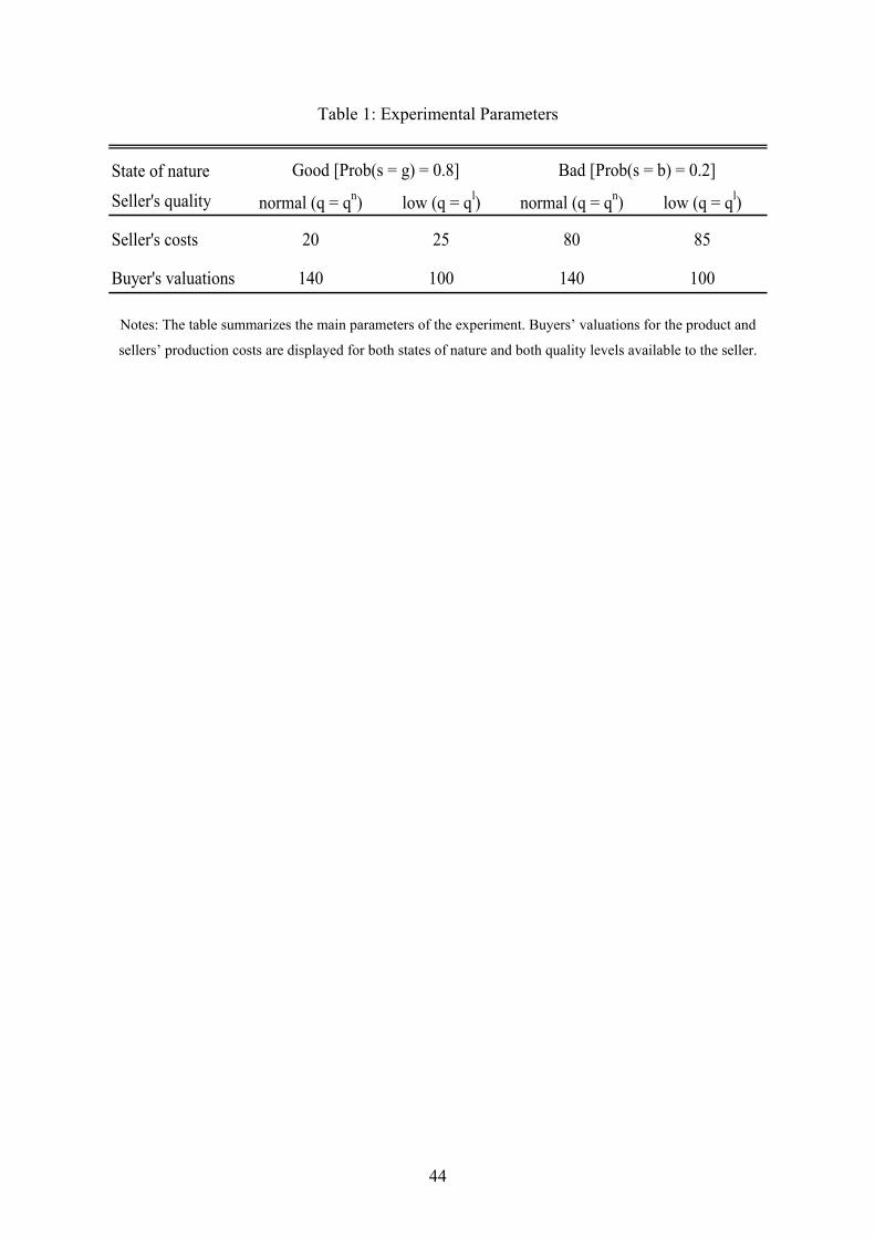
44

Table 1: Experimental Parameters

State of nature

Seller's quality normal (q = qn) low (q = ql) normal (q = qn) low (q = ql)

Seller's costs 20 25 80 85

Buyer's valuations 140 100 140 100

Good [Prob(s = g) = 0.8] Bad [Prob(s = b) = 0.2]

Notes: The table summarizes the main parameters of the experiment. Buyers’ valuations for the product and

sellers’ production costs are displayed for both states of nature and both quality levels available to the seller.

45

Table 2 (Informal Agreements / Baseline): Comparison of Contracts

Contract

State Good Bad Good Bad Good Bad Good Bad

Average Price 39.8 - 47.8 97.9 40.7 - 51.1 98.4

Rel. Freq. of Shading 0.05 - 0.13 0.21 0.06 - 0.25 0.30

Av. Auction Outcomce

Average Profit Buyer 98.2 10.0 87.3 33.9 96.8 10.0 79.9 29.7

Average Profit Seller 19.5 10.0 27.2 16.8 20.4 10.0 29.8 16.9

Number of Observations 201 59 539 131 398 111 407 104

76.9 77.9 68.9

Rigid

Informal Agreement Baseline

25.1 18.1 27.2

39.8

78.2

17.4

FlexibleRigidFlexible

38.7 40.7 40.2

Notes: The table summarizes the outcomes for rigid and flexible contracts in both states of nature. “Average

Price” is the average of the trading price and “Relative Frequency of Shading” measures how often the seller has

chosen the low quality. For rigid contracts this information is available only for the good state, because trade

does not occur in the bad state. “Average Auction Outcome” is the average of the fixed price in case of rigid

contracts and the lower bound of the price range in case of flexible contracts. “Average Profit Buyer (Seller)”

measures the average payoff of buyers (sellers) for each (state and) contract. In rigid contracts the payoffs in the

bad state of the world are the outside options of the market participants.

46

Table 3 (Informal Agreements): Trade-off Between Contractual Rigidity and Flexibility

Dependent Variable Price Shading Shading Profit ProfitState Good Good Good Good Good&Bad

OLS Probit Probit OLS OLS(1) (2) (3) (4) (5)

Flexible contract 7.993** 0.073*** 0.082*** -10.901** -1.326(2.608) (0.018) (0.025) (3.198) (4.033)

Price -0.002**(0.001)

Constant 39.771*** 98.239*** 78.215***(0.664) (0.877) (2.231)

Observation 740 740 740 740 930

R2 0.090 0.086 0.000

Notes: “Flexible contract” is an indicator variable which is unity if the contract is of the flexible type and

zero otherwise. Columns (1), (4) and (5) report coefficients of OLS estimations. Columns (2) and (3) report

marginal effects based on Probit estimations. Since observations within sessions may be dependent all

reported standard errors are adjusted for clustering at the session level. *** p<0.01, ** p<0.05, * p<0.1.

47

Table 4 (Informal Agreements): Effects of Informal Agreements

Dep. Variable Shading Shading Shading Shading Shading ShadingState Good Bad Good Bad Good Bad

Probit Probit Probit Probit Probit Probit(1) (2) (3) (4) (5) (6)

Price -0.004 -0.027*** -0.001 -0.017** -0.004* -0.017***(0.003) (0.008) (0.003) (0.010) (0.002) (0.008)

Price Announc. 0.003*** 0.008(0.001) (0.007)

Violation of IA 0.131*** 0.382**(0.077) (0.216)

Low PA 0.002 0.019(0.033) (0.046)

High PA 0.069*** 0.127(0.033) (0.150)

Observation 256 59 256 59 539 131

Notes: “Violation of IA” is an indicator variable which is unity if the buyer picks a final price which is below

his price announcement. “Low PA” is an indicator variable which is unity if the buyer announced low prices

for both states (i.e., price announcement ≤ 40 in the good state, and price announcement ≤ 100 in the bad

state). “High PA” is an indicator variable which is unity if the buyer announced a high price for at least one

state (i.e., price announcement > 40 in the good state, or price announcement > 100 in the bad state). All

columns report marginal effects based on Probit estimations. Since observations within sessions may be

dependent, all reported standard errors are adjusted for clustering at the session level. *** p<0.01, ** p<0.05,

* p<0.1.

48

Table 5 (Informal Agreements): Prices, Shading, and Buyer Profits Across Contracts

Contract

State Good Bad Good Bad Good Bad Good Bad

Average Price 39.8 - 45.7 96.8 44.5 97.9 52.0 99.5

Rel. Freq. of Shading 0.05 - 0.11 0.18 0.11 0.14 0.15 0.27

Av. Auction Outcome

Average Profit Buyer 98.2 10.0 90.1 35.9 91.2 36.4 81.9 29.8

Average Profit Seller 19.5 10.0 25.1 15.9 24.0 17.1 31.3 18.2

Number of Observations 201 59 283 72 66 14 190 45

23.3 22.8 28.8

39.8

78.2

Rigid

17.4

HighPALowPANoPA

Flexible

39.1 38.6 38.4

79.1 81.6 71.9

Notes: “NoPA” stands for “no price announcement”. “LowPA” represents contracts, in which the buyer

announced low prices for both states (i.e., price ≤ 40 in the good state, and price ≤ 100 in the bad state).

“HighPA” contains contracts, in which the buyer announced a high price for at least one state (i.e., price > 40 in

the good state, or price > 100 in the bad state). For descriptions of the variables please see the notes of Table 2.

49

Table 6 (Renegotiation / Baseline): Comparison of Non-Renegotiated Contracts

Contract

State Good Bad Good Bad Good Bad Good Bad

Average Price 38.5 - 42.2 96.1 40.7 - 51.1 98.4

Rel. Freq. of Shading 0.04 - 0.09 0.11 0.06 - 0.25 0.30

Av. Auction Outcomce

Average Profit Buyer 99.8 10.0 94.4 39.4 96.8 10.0 79.9 29.7

(weighted average)

Average Profit Seller 18.3 10.0 21.7 15.5 20.4 10.0 29.8 16.9

(weighted average)

Number of Observations 282 20 418 79 398 111 407 104

Rigid

Renegotiation Baseline

FlexibleRigidFlexible

20.5 18.3 27.2

38.6

81.8

16.6

37.3 40.7 40.2

83.4 79.4 69.9

Notes: See the notes of Table 2 for a detailed description of all variables. Since renegotiation is not equally

likely in the good and the bad state, we do not compare observed overall profits (the empirical weights are

distorted). Instead we provide weighted averages of profits in the good and the bad state of the world (using the

theoretical probabilities for the realization of each state).

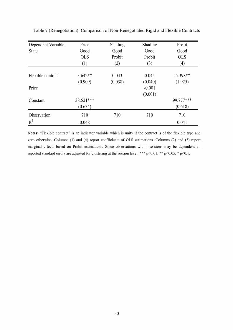
50

Table 7 (Renegotiation): Comparison of Non-Renegotiated Rigid and Flexible Contracts

Dependent Variable Price Shading Shading ProfitState Good Good Good Good

OLS Probit Probit OLS(1) (2) (3) (4)

Flexible contract 3.642** 0.043 0.045 -5.398**(0.909) (0.038) (0.040) (1.925)

Price -0.001(0.001)

Constant 38.521*** 99.777***(0.634) (0.618)

Observation 710 710 710 710

R2 0.048 0.041

Notes: “Flexible contract” is an indicator variable which is unity if the contract is of the flexible type and

zero otherwise. Columns (1) and (4) report coefficients of OLS estimations. Columns (2) and (3) report

marginal effects based on Probit estimations. Since observations within sessions may be dependent all

reported standard errors are adjusted for clustering at the session level. *** p<0.01, ** p<0.05, * p<0.1.

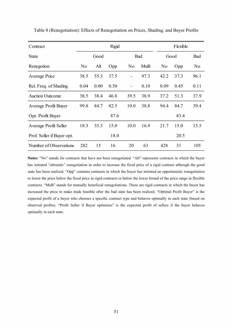
51

Table 8 (Renegotiation): Effects of Renegotiation on Prices, Shading, and Buyer Profits

Contract

State Bad

Renegotion No Alt Opp No MuB No Opp No

Average Price 38.5 55.3 37.5 - 97.3 42.2 37.3 96.1

Rel. Freq. of Shading 0.04 0.00 0.50 - 0.10 0.09 0.45 0.11

Auction Outcome 38.5 38.4 46.8 39.5 38.9 37.2 51.3 37.9

Average Profit Buyer 99.8 84.7 82.5 10.0 38.8 94.4 84.7 39.4

Opt. Profit Buyer

Average Profit Seller 18.3 35.3 15.0 10.0 16.9 21.7 15.0 15.5

Prof. Seller if Buyer opt.

Number of Observations 282 15 16 20 63 428 31 105

18.0 20.5

Good

Flexible

BadGood

Rigid

87.6 83.4

Notes: “No” stands for contracts that have not been renegotiated. “Alt” represents contracts in which the buyer

has initiated “altruistic” renegotiation in order to increase the fixed price of a rigid contract although the good

state has been realized. “Opp” contains contracts in which the buyer has initiated an opportunistic renegotiation

to lower the price below the fixed price in rigid contracts or below the lower bound of the price range in flexible

contracts. “MuB” stands for mutually beneficial renegotiations. These are rigid contracts in which the buyer has

increased the price to make trade feasible after the bad state has been realized. “Optimal Profit Buyer” is the

expected profit of a buyer who chooses a specific contract type and behaves optimally in each state (based on

observed profits). “Profit Seller if Buyer optimizes” is the expected profit of sellers if the buyer behaves

optimally in each state.

52

Table 9 (Renegotiation): Effects of Mutually Beneficial Renegotiations

Dependent Variable Price Shading Shading ProfitState Bad Bad Bad Bad

OLS Probit Probit OLS(1) (2) (3) (4)

Flexible contract -1.273 0.019 0.000 0.511(0.692) (0.079) (0.080) (2.956)

Price -0.015*(0.013)

Constant 97.349*** 38.841***(0.835) (3.512)

Observation 168 168 168 168

R2 0.039 0.000

Notes: “Flexible contract” is an indicator variable which is unity if the contract is of the flexible type and

zero otherwise. Columns (1) and (4) report coefficients of OLS estimations. Columns (2) and (3) report

marginal effects based on Probit estimations. Since observations within sessions may be dependent all

reported standard errors are adjusted for clustering at the session level. *** p<0.01, ** p<0.05, * p<0.1.

53

Table 10 (Renegotiation): Effects of Opportunistic Renegotiations

Dep. Variable Shading Shading Profit ProfitState Good Good Good GoodContract Rigid Flexible Rigid Flexible

Probit Probit OLS OLS(1) (2) (3) (4)

Price -0.002 -0.002 -1.114*** -0.951***(0.002) (0.002) (0.119) (0.057)

Opp. Reneg. 0.469*** 0.350*** -18.414* -14.368***(0.168) (0.029) (7.010) (1.031)

Auction Outc.

Constant 142.679*** 134.488***(4.093) (2.793)

Observations 298 459 298 459

R2 0.415 0.342

Notes: “Opportunistic Renegotiation” is an indicator variable which is unity if the buyer has initiated

renegotiation in the good state of the world to either lower the price to a level below the fixed price of a rigid

contract or the lower bound of the price range in a flexible contract. Columns (1) and (2) report marginal

effects based on Probit estimations. Columns (3) and (4) report coefficients of OLS estimations. Since

observations within sessions may be dependent, all reported standard errors are adjusted for clustering at the

session level. *** p<0.01, ** p<0.05, * p<0.1.