hermitian compact operators on the cubed-sphere -...
TRANSCRIPT
—
HERMITIAN COMPACT OPERATORS ONTHE CUBED-SPHERE
Jean-Pierre Croisille
Departement de mathematiques
Universite de Lorraine - Metz, France
National Center for Atmospheric Research
April 27, 2012
Jean-Pierre CROISILLE - Universite de Lorraine - Metz, France NCAR - April 27, 2012

Outline
1 The Cubed-Sphere Grid
2 Three-point Hermitian Derivative in one-dimension
3 Hermitian derivatives on great circles
4 Approximate high-order spherical gradient
5 The cosine-bell advection test-case
6 A high-order eigenvalue problem on the sphere.
Jean-Pierre CROISILLE - Universite de Lorraine - Metz, France NCAR - April 27, 2012
The Cubed-Sphere grid(1)
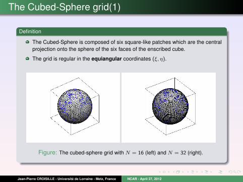
Definition
The Cubed-Sphere is composed of six square-like patches which are the centralprojection onto the sphere of the six faces of the enscribed cube.
The grid is regular in the equiangular coordinates (ξ, η).
Figure: The cubed-sphere grid with N = 16 (left) and N = 32 (right).
Jean-Pierre CROISILLE - Universite de Lorraine - Metz, France NCAR - April 27, 2012
The Cubed-Sphere grid(2)
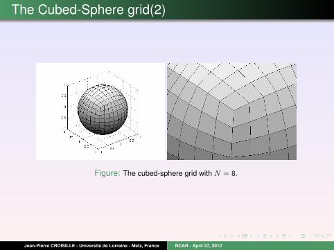
Figure: The cubed-sphere grid with N = 8.
Jean-Pierre CROISILLE - Universite de Lorraine - Metz, France NCAR - April 27, 2012
The Cubed-Sphere grid(3)
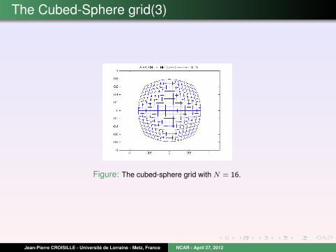
Figure: The cubed-sphere grid with N = 16.
Jean-Pierre CROISILLE - Universite de Lorraine - Metz, France NCAR - April 27, 2012
The Cubed-Sphere grid(4)
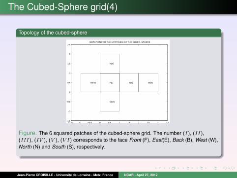
Topology of the cubed-sphere
−1.5 −1 −0.5 0 0.5 1 1.5 2 2.5 3 3.5−1.5
−1
−0.5
0
0.5
1
1.5
2
2.5
F(I) E(II) B(III)W(IV)
N(V)
S(VI)
NOTATION FOR THE 6 PATCHES OF THE CUBED−SPHERE
Figure: The 6 squared patches of the cubed-sphere grid. The number (I), (II),(III), (IV ), (V ), (V I) corresponds to the face Front (F), East(E), Back (B), West (W),North (N) and South (S), respectively.
Jean-Pierre CROISILLE - Universite de Lorraine - Metz, France NCAR - April 27, 2012
Coordinate systems on the cubed-sphere grid
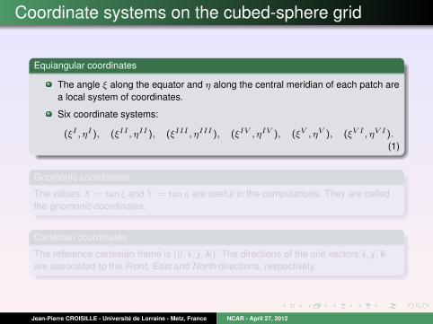
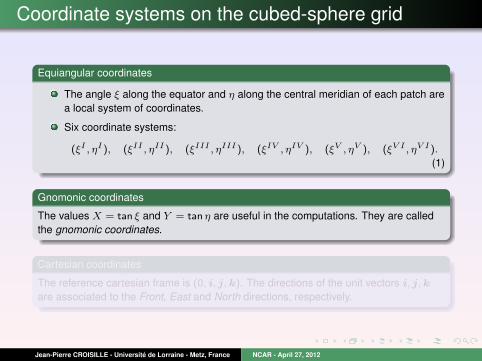
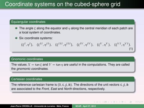
Equiangular coordinates
The angle ξ along the equator and η along the central meridian of each patch area local system of coordinates.
Six coordinate systems:
(ξI , ηI), (ξII , ηII), (ξIII , ηIII), (ξIV , ηIV ), (ξV , ηV ), (ξV I , ηV I).
(1)
Gnomonic coordinates
The values X = tan ξ and Y = tan η are useful in the computations. They are calledthe gnomonic coordinates.
Cartesian coordinates
The reference cartesian frame is (0, i, j, k). The directions of the unit vectors i, j, k
are associated to the Front, East and North directions, respectively.
Jean-Pierre CROISILLE - Universite de Lorraine - Metz, France NCAR - April 27, 2012
Coordinate systems on the cubed-sphere grid
Equiangular coordinates
The angle ξ along the equator and η along the central meridian of each patch area local system of coordinates.
Six coordinate systems:
(ξI , ηI), (ξII , ηII), (ξIII , ηIII), (ξIV , ηIV ), (ξV , ηV ), (ξV I , ηV I).
(1)
Gnomonic coordinates
The values X = tan ξ and Y = tan η are useful in the computations. They are calledthe gnomonic coordinates.
Cartesian coordinates
The reference cartesian frame is (0, i, j, k). The directions of the unit vectors i, j, k
are associated to the Front, East and North directions, respectively.
Jean-Pierre CROISILLE - Universite de Lorraine - Metz, France NCAR - April 27, 2012
Grid functions on the cubed-sphere
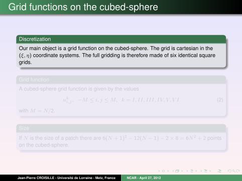
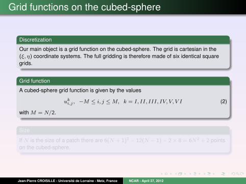
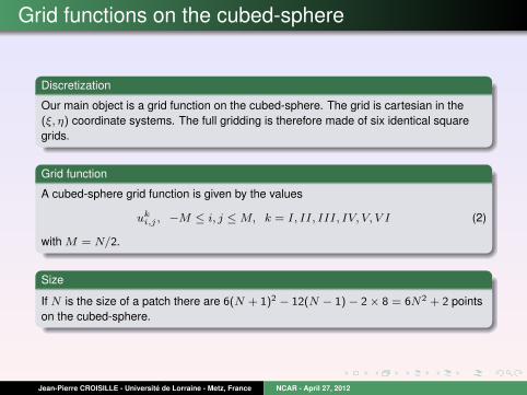
Discretization
Our main object is a grid function on the cubed-sphere. The grid is cartesian in the(ξ, η) coordinate systems. The full gridding is therefore made of six identical squaregrids.
Grid function
A cubed-sphere grid function is given by the values
uki,j , −M ≤ i, j ≤ M, k = I, II, III, IV, V, V I (2)
with M = N/2.
Size
If N is the size of a patch there are 6(N + 1)2 − 12(N − 1)− 2× 8 = 6N2 + 2 pointson the cubed-sphere.
Jean-Pierre CROISILLE - Universite de Lorraine - Metz, France NCAR - April 27, 2012
Grid functions on the cubed-sphere
Discretization
Our main object is a grid function on the cubed-sphere. The grid is cartesian in the(ξ, η) coordinate systems. The full gridding is therefore made of six identical squaregrids.
Grid function
A cubed-sphere grid function is given by the values
uki,j , −M ≤ i, j ≤ M, k = I, II, III, IV, V, V I (2)
with M = N/2.
Size
If N is the size of a patch there are 6(N + 1)2 − 12(N − 1)− 2× 8 = 6N2 + 2 pointson the cubed-sphere.
Jean-Pierre CROISILLE - Universite de Lorraine - Metz, France NCAR - April 27, 2012
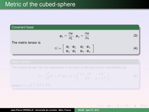
Metric of the cubed-sphere
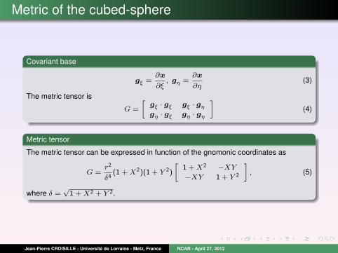
Covariant base
gξ =∂x
∂ξ, gη =
∂x
∂η(3)
The metric tensor is
G =
»gξ · gξ gξ · gη
gη · gξ gη · gη
–(4)
Metric tensor
The metric tensor can be expressed in function of the gnomonic coordinates as
G =r2
δ4(1 + X2)(1 + Y 2)
»1 + X2 −XY
−XY 1 + Y 2
–, (5)
where δ =√
1 + X2 + Y 2.
Jean-Pierre CROISILLE - Universite de Lorraine - Metz, France NCAR - April 27, 2012
Metric of the cubed-sphere
Covariant base
gξ =∂x
∂ξ, gη =
∂x
∂η(3)
The metric tensor is
G =
»gξ · gξ gξ · gη
gη · gξ gη · gη
–(4)
Metric tensor
The metric tensor can be expressed in function of the gnomonic coordinates as
G =r2
δ4(1 + X2)(1 + Y 2)
»1 + X2 −XY
−XY 1 + Y 2
–, (5)
where δ =√
1 + X2 + Y 2.
Jean-Pierre CROISILLE - Universite de Lorraine - Metz, France NCAR - April 27, 2012
Metric of the cubed-sphere (2)
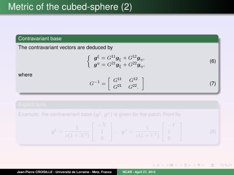
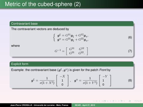
Contravariant base
The contravariant vectors are deduced bygξ = G11gξ + G12gη ,
gη = G21gξ + G22gη ,(6)
where
G−1 =
»G11 G12
G21 G22.
–(7)
Explicit form
Example: the contravariant base (gξ, gη) is given for the patch Front by
gξ =1
x(1 + X2)
24 −X
1
0
35 , gη =1
x(1 + Y 2)
24 −Y
1
0
35 (8)
Jean-Pierre CROISILLE - Universite de Lorraine - Metz, France NCAR - April 27, 2012
Metric of the cubed-sphere (2)
Contravariant base
The contravariant vectors are deduced bygξ = G11gξ + G12gη ,
gη = G21gξ + G22gη ,(6)
where
G−1 =
»G11 G12
G21 G22.
–(7)
Explicit form
Example: the contravariant base (gξ, gη) is given for the patch Front by
gξ =1
x(1 + X2)
24 −X
1
0
35 , gη =1
x(1 + Y 2)
24 −Y
1
0
35 (8)
Jean-Pierre CROISILLE - Universite de Lorraine - Metz, France NCAR - April 27, 2012
Three-point Hermitian Derivative Operator
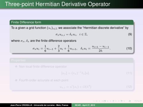
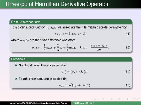
Finite Difference form
To a given a grid function (ui)i∈Z we associate the “Hermitian discrete derivative” by
σxux,i = δxui, i ∈ Z, (9)
where σx, δx are the finite difference operators
σxui =1
6ui−1 +
2
3ui +
1
6ui+1, δxui =
ui+1 − ui−1
2h. (10)
Properties
Non local finite difference operator
[ux] = (σx)−1δx[u]. (11)
Fourth-order accurate at each point
ux,i = u′(xi) + O(h4) (12)
Jean-Pierre CROISILLE - Universite de Lorraine - Metz, France NCAR - April 27, 2012
Three-point Hermitian Derivative Operator
Finite Difference form
To a given a grid function (ui)i∈Z we associate the “Hermitian discrete derivative” by
σxux,i = δxui, i ∈ Z, (9)
where σx, δx are the finite difference operators
σxui =1
6ui−1 +
2
3ui +
1
6ui+1, δxui =
ui+1 − ui−1
2h. (10)
Properties
Non local finite difference operator
[ux] = (σx)−1δx[u]. (11)
Fourth-order accurate at each point
ux,i = u′(xi) + O(h4) (12)
Jean-Pierre CROISILLE - Universite de Lorraine - Metz, France NCAR - April 27, 2012
Hermitian Derivative Operator on an irregular periodicgrid
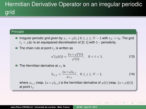
Principle
Irregular periodic grid given by xj = ϕ(tj) 0 ≤ j ≤ N − 1 with tN = t0. The gridtj = j∆t is an equispaced discretisation of [0, 1] with 1− periodicity.
The chain rule at point tj is written as
u′(ϕ(t)) =(u ◦ ϕ)′(t)
ϕ′(t), 0 < t < 1. (13)
The Hermitian derivative at xj is
ux,j =(u ◦ ϕ)t,j
ϕt,j, 0 ≤ j ≤ N − 1, (14)
where ϕt,j (resp. (u ◦ ϕ)t,j ) is the hermitian derivative of ϕ(t) (resp. (u ◦ ϕ)(t))
at point tj .
Jean-Pierre CROISILLE - Universite de Lorraine - Metz, France NCAR - April 27, 2012
Coordinate great circles
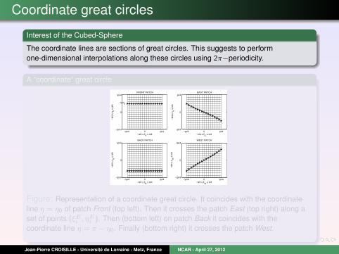
Interest of the Cubed-Sphere
The coordinate lines are sections of great circles. This suggests to performone-dimensional interpolations along these circles using 2π−periodicity.
A “coordinate” great circle
−pi/4 0 pi/4−\pi/4
0
\pi/4
−π/4 ≤ ξF ≤ π/4
−π/
4 ≤
η F ≤
π/4
FRONT PATCH
η=η0
−pi/4 0 pi/4−pi/4
0
pi/4
−π/4 ≤ ξE ≤ π/4
−π/
4 ≤
η E ≤
π/4
EAST PATCH
−\pi/4 0 \pi/4−\pi/4
0
\pi/4
−π/4 ≤ ξB ≤ π/4
−π/
4 ≤
η B ≤
π/4
BACK PATCH
−\pi/4 0 \pi/4−\pi/4
0
\pi/4
−π/4 ≤ ξW
≤ π/4
−π/
4 ≤
η W ≤
π/4
WEST PATCH
Figure: Representation of a coordinate great circle. It coincides with the coordinateline η = η0 of patch Front (top left). Then it crosses the patch East (top right) along aset of points (ξE
i , ηEi ). Then (bottom left) on patch Back it coincides with the
coordinate line η = π − η0. Finally (bottom right) it crosses the patch West.
Jean-Pierre CROISILLE - Universite de Lorraine - Metz, France NCAR - April 27, 2012
Coordinate great circles
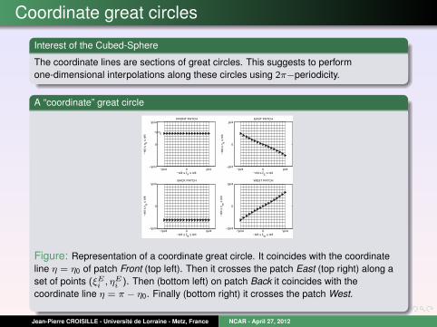
Interest of the Cubed-Sphere
The coordinate lines are sections of great circles. This suggests to performone-dimensional interpolations along these circles using 2π−periodicity.
A “coordinate” great circle
−pi/4 0 pi/4−\pi/4
0
\pi/4
−π/4 ≤ ξF ≤ π/4
−π/
4 ≤
η F ≤
π/4
FRONT PATCH
η=η0
−pi/4 0 pi/4−pi/4
0
pi/4
−π/4 ≤ ξE ≤ π/4
−π/
4 ≤
η E ≤
π/4
EAST PATCH
−\pi/4 0 \pi/4−\pi/4
0
\pi/4
−π/4 ≤ ξB ≤ π/4
−π/
4 ≤
η B ≤
π/4
BACK PATCH
−\pi/4 0 \pi/4−\pi/4
0
\pi/4
−π/4 ≤ ξW
≤ π/4
−π/
4 ≤
η W ≤
π/4
WEST PATCH
Figure: Representation of a coordinate great circle. It coincides with the coordinateline η = η0 of patch Front (top left). Then it crosses the patch East (top right) along aset of points (ξE
i , ηEi ). Then (bottom left) on patch Back it coincides with the
coordinate line η = π − η0. Finally (bottom right) it crosses the patch West.
Jean-Pierre CROISILLE - Universite de Lorraine - Metz, France NCAR - April 27, 2012
Networks of great circles on the cubed-sphere
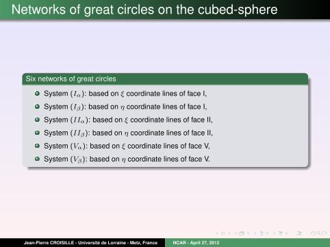
Six networks of great circles
System (Iα): based on ξ coordinate lines of face I,
System (Iβ): based on η coordinate lines of face I,
System (IIα): based on ξ coordinate lines of face II,
System (IIβ): based on η coordinate lines of face II,
System (Vα): based on ξ coordinate lines of face V,
System (Vβ): based on η coordinate lines of face V.
Jean-Pierre CROISILLE - Universite de Lorraine - Metz, France NCAR - April 27, 2012
Networks of great circles on the cubed-sphere
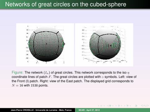
Figure: The network (Iα) of great circles. This network corresponds to the iso η
coordinate lines of patch F . The great circles are plotted with o symbols. Left: view ofthe Front (I) patch. Right: view of the East patch. The displayed grid corresponds toN = 16 with 1538 points.
Jean-Pierre CROISILLE - Universite de Lorraine - Metz, France NCAR - April 27, 2012
Computing the spherical gradient
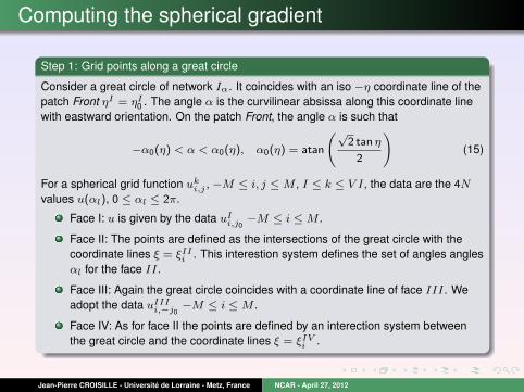
Step 1: Grid points along a great circle
Consider a great circle of network Iα. It coincides with an iso −η coordinate line of thepatch Front ηI = ηI
0 . The angle α is the curvilinear absissa along this coordinate linewith eastward orientation. On the patch Front, the angle α is such that
−α0(η) < α < α0(η), α0(η) = atan
√2 tan η
2
!(15)
For a spherical grid function uki,j , −M ≤ i, j ≤ M , I ≤ k ≤ V I, the data are the 4N
values u(αl), 0 ≤ αl ≤ 2π.
Face I: u is given by the data uIi,j0
−M ≤ i ≤ M .
Face II: The points are defined as the intersections of the great circle with thecoordinate lines ξ = ξII
i . This interestion system defines the set of angles anglesαl for the face II.
Face III: Again the great circle coincides with a coordinate line of face III. Weadopt the data uIII
i,−j0−M ≤ i ≤ M .
Face IV: As for face II the points are defined by an interection system betweenthe great circle and the coordinate lines ξ = ξIV
i .
Jean-Pierre CROISILLE - Universite de Lorraine - Metz, France NCAR - April 27, 2012
Computing the spherical gradient (2)
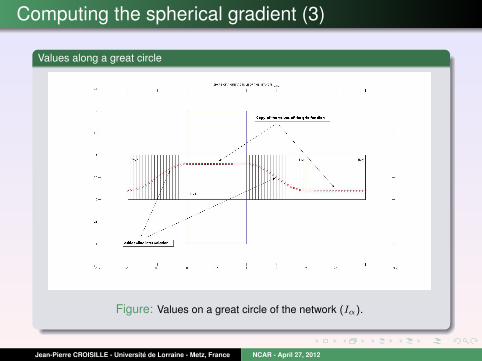
Step 2: Assembling values along a great circle
On faces II (East) and IV (West), the values at the points of the great circle are given byan interpolation. Along each “vertical” coordinate lines ξ = ξII
i , −M ≤ i ≤ M , weadopt a cubic spline interpolation. End values are specified (for example) by the “not aknot” condition.
Jean-Pierre CROISILLE - Universite de Lorraine - Metz, France NCAR - April 27, 2012
Computing the spherical gradient (3)
Values along a great circle
Figure: Values on a great circle of the network (Iα).
Jean-Pierre CROISILLE - Universite de Lorraine - Metz, France NCAR - April 27, 2012
Computing the spherical gradient (4)
Step3: Hermitian derivatives along a great circle
Using discrete one-dimensional periodic data along the great circle, allows to evaluatethe hermitian gradient. This gives a “fourth order” accurate approximation of thederivative along the circle.
Hermitian derivatives for six networks of great circles
As a result we obtain on each patch I, II, III, IV, V, V I approximations of thederivatives 8>><>>:
∂u(α, η)
∂α |η,
∂u(ξ, β)
∂β |ξ
(16)
Jean-Pierre CROISILLE - Universite de Lorraine - Metz, France NCAR - April 27, 2012
Computing the spherical gradient(5)
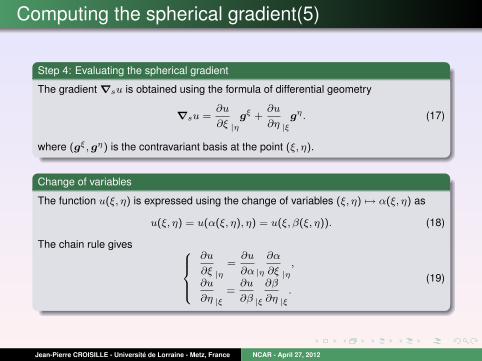
Step 4: Evaluating the spherical gradient
The gradient ∇su is obtained using the formula of differential geometry
∇su =∂u
∂ξ |ηgξ +
∂u
∂η |ξgη . (17)
where (gξ, gη) is the contravariant basis at the point (ξ, η).
Change of variables
The function u(ξ, η) is expressed using the change of variables (ξ, η) 7→ α(ξ, η) as
u(ξ, η) = u(α(ξ, η), η) = u(ξ, β(ξ, η)). (18)
The chain rule gives 8>><>>:∂u
∂ξ |η=
∂u
∂α |η
∂α
∂ξ |η,
∂u
∂η |ξ=
∂u
∂β |ξ
∂β
∂η |ξ.
(19)
Jean-Pierre CROISILLE - Universite de Lorraine - Metz, France NCAR - April 27, 2012
Computing the spherical gradient(5)
Step 4: Evaluating the spherical gradient
The gradient ∇su is obtained using the formula of differential geometry
∇su =∂u
∂ξ |ηgξ +
∂u
∂η |ξgη . (17)
where (gξ, gη) is the contravariant basis at the point (ξ, η).
Change of variables
The function u(ξ, η) is expressed using the change of variables (ξ, η) 7→ α(ξ, η) as
u(ξ, η) = u(α(ξ, η), η) = u(ξ, β(ξ, η)). (18)
The chain rule gives 8>><>>:∂u
∂ξ |η=
∂u
∂α |η
∂α
∂ξ |η,
∂u
∂η |ξ=
∂u
∂β |ξ
∂β
∂η |ξ.
(19)
Jean-Pierre CROISILLE - Universite de Lorraine - Metz, France NCAR - April 27, 2012
Computing the spherical gradient(6)
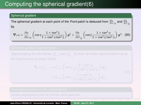
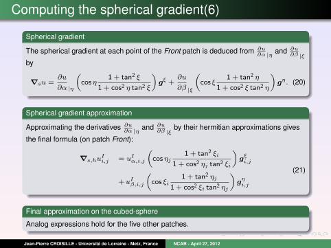
Spherical gradient
The spherical gradient at each point of the Front patch is deduced from ∂u∂α |η and ∂u
∂β |ξby
∇su =∂u
∂α |η
„cos η
1 + tan2 ξ
1 + cos2 η tan2 ξ
«gξ +
∂u
∂β |ξ
„cos ξ
1 + tan2 η
1 + cos2 ξ tan2 η
«gη . (20)
Spherical gradient approximation
Approximating the derivatives ∂u∂α |η and ∂u
∂β |ξby their hermitian approximations gives
the final formula (on patch Front):
∇s,huIi,j = uI
α,i,j
„cos ηj
1 + tan2 ξi
1 + cos2 ηj tan2 ξi
«gξ
i,j
+ uIβ,i,j
„cos ξi
1 + tan2 ηj
1 + cos2 ξi tan2 ηj
«gη
i,j
(21)
Final approximation on the cubed-sphere
Analog expressions hold for the five other patches.
Jean-Pierre CROISILLE - Universite de Lorraine - Metz, France NCAR - April 27, 2012
Computing the spherical gradient(6)
Spherical gradient
The spherical gradient at each point of the Front patch is deduced from ∂u∂α |η and ∂u
∂β |ξby
∇su =∂u
∂α |η
„cos η
1 + tan2 ξ
1 + cos2 η tan2 ξ
«gξ +
∂u
∂β |ξ
„cos ξ
1 + tan2 η
1 + cos2 ξ tan2 η
«gη . (20)
Spherical gradient approximation
Approximating the derivatives ∂u∂α |η and ∂u
∂β |ξby their hermitian approximations gives
the final formula (on patch Front):
∇s,huIi,j = uI
α,i,j
„cos ηj
1 + tan2 ξi
1 + cos2 ηj tan2 ξi
«gξ
i,j
+ uIβ,i,j
„cos ξi
1 + tan2 ηj
1 + cos2 ξi tan2 ηj
«gη
i,j
(21)
Final approximation on the cubed-sphere
Analog expressions hold for the five other patches.
Jean-Pierre CROISILLE - Universite de Lorraine - Metz, France NCAR - April 27, 2012
Accuracy of the calculated gradient
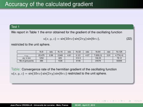
Test 1
We report in Table 1 the error obtained for the gradient of the oscillating function
u(x, y, z) = sin(10πx) sin(2πy) sin(6πz), (22)
restricted to the unit sphere.
N=8 rate N=16 rate N=32 rate N=64 rate N=128
e∞ 23.475 2.99 2.949 4.61 0.121 4.07 7.205(-3) 3.91 4.774(-4)∆ξ in km 1250 625 312.5 156.25 78.12
Nb of grid points 386 1538 6146 24578 93306
Table: Convergence rate of the hermitian gradient of the oscillating functionu(x, y, z) = sin(10πx) sin(2πy) sin(6πz) restricted to the unit sphere.
Jean-Pierre CROISILLE - Universite de Lorraine - Metz, France NCAR - April 27, 2012
Accuracy of the calculated gradient (2)
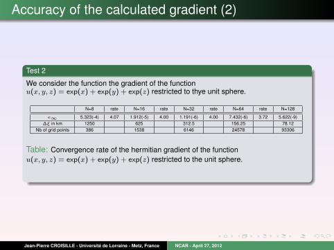
Test 2
We consider the function the gradient of the functionu(x, y, z) = exp(x) + exp(y) + exp(z) restricted to thye unit sphere.
N=8 rate N=16 rate N=32 rate N=64 rate N=128
e∞ 5.323(-4) 4.07 1.912(-5) 4.00 1.191(-6) 4.00 7.432(-6) 3.72 5.622(-9)∆ξ in km 1250 625 312.5 156.25 78.12
Nb of grid points 386 1538 6146 24578 93306
Table: Convergence rate of the hermitian gradient of the functionu(x, y, z) = exp(x) + exp(y) + exp(z) restricted to the unit sphere.
Jean-Pierre CROISILLE - Universite de Lorraine - Metz, France NCAR - April 27, 2012
Cosine-bell test case (D. Williamson et al.)
Advection equation on the sphere
Test problem : propagation of a cosine-bell at constant solide spherical velocityaround the earth.
Serves as a preliminary test to evaluate the accuracy of numerical methods forthe shallow water system
Reference results widely reported in the literature by various kinds of spatialapproximations: spectral, FV MUSCL, SE, DG, etc, on various grids:longitude/latitude, icosahedral, cubed-sphere, etc.
Setting of the problem
h(x, t)=height of the bell. ∂th(x, t) + c · ∇sh(x, t) = 0
h(x, 0) = h0(x)(23)
The velocity is a “constant” solid velocity.
Jean-Pierre CROISILLE - Universite de Lorraine - Metz, France NCAR - April 27, 2012
The Cosine-Bell at initial position
−5
0
5
x 106
−6−4
−20
24
6
x 106
−6
−4
−2
0
2
4
6
x 106
F
W
S
N
E
B
0
100
200
300
400
500
600
700
800
900
1000
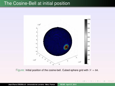
Figure: Initial position of the cosine-bell. Cubed-sphere grid with N = 64.
Jean-Pierre CROISILLE - Universite de Lorraine - Metz, France NCAR - April 27, 2012
Spatial approximation
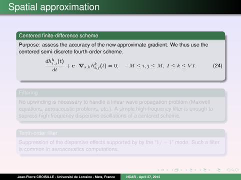
Centered finite-difference scheme
Purpose: assess the accuracy of the new approximate gradient. We thus use thecentered semi-discrete fourth-order scheme.
dhki,j(t)
dt+ c ·∇s,hhk
i,j(t) = 0, −M ≤ i, j ≤ M, I ≤ k ≤ V I. (24)
Filtering
No upwinding is necessary to handle a linear wave propagation problem (Maxwellequations, aeroacoustic problems, etc.). A simple high-frequency filter is enough tosupress high-frequency dispersive oscillations of a centered scheme.
Tenth-order filter
Suppression of the dispersive effects supported by by the “1/− 1” mode. Such a filteris common in aeroacoustics computations.
Jean-Pierre CROISILLE - Universite de Lorraine - Metz, France NCAR - April 27, 2012

Spatial approximation
Centered finite-difference scheme
Purpose: assess the accuracy of the new approximate gradient. We thus use thecentered semi-discrete fourth-order scheme.
dhki,j(t)
dt+ c ·∇s,hhk
i,j(t) = 0, −M ≤ i, j ≤ M, I ≤ k ≤ V I. (24)
Filtering
No upwinding is necessary to handle a linear wave propagation problem (Maxwellequations, aeroacoustic problems, etc.). A simple high-frequency filter is enough tosupress high-frequency dispersive oscillations of a centered scheme.
Tenth-order filter
Suppression of the dispersive effects supported by by the “1/− 1” mode. Such a filteris common in aeroacoustics computations.
Jean-Pierre CROISILLE - Universite de Lorraine - Metz, France NCAR - April 27, 2012
Filtering the 1/− 1 mode
Filtering of a grid function
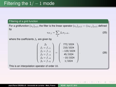
For a gridfunction (uj)j∈Z the filter is the linear operator (uj)j∈Z 7→ (uF,j)j∈Z definedby
uF,j =X
k
fkuj+k, (25)
where the coefficients fk are given by0BBBBBBB@
f0
f1 = f−1
f2 = f−2
f3 = f−3
f4 = f−4
f5 = f−5
1CCCCCCCA=
0BBBBBBB@
772/1024
210/1024
−120/1024
45/1024
−10/1024
1/1024
1CCCCCCCA. (26)
This is an interpolation operator of order 10.
Jean-Pierre CROISILLE - Universite de Lorraine - Metz, France NCAR - April 27, 2012
Fourth-order time-stepping scheme
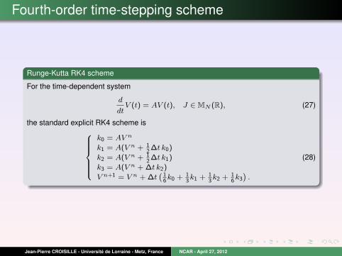
Runge-Kutta RK4 scheme
For the time-dependent system
d
dtV (t) = AV (t), J ∈ MN (R), (27)
the standard explicit RK4 scheme is8>>>><>>>>:k0 = AV n
k1 = A(V n + 12∆t k0)
k2 = A(V n + 12∆t k1)
k3 = A(V n + ∆t k2)
V n+1 = V n + ∆t`
16k0 + 1
3k1 + 1
3k2 + 1
6k3
´.
(28)
Jean-Pierre CROISILLE - Universite de Lorraine - Metz, France NCAR - April 27, 2012
Cosine-bell test case: numerical results (1)
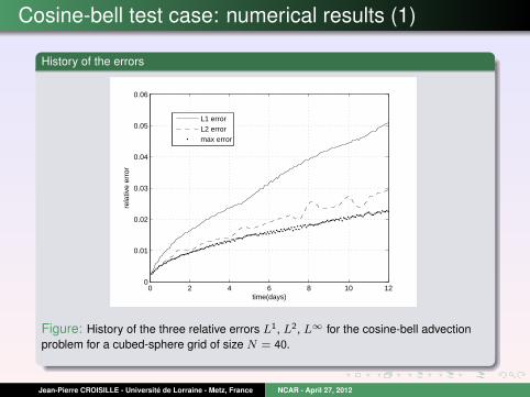
History of the errors
0 2 4 6 8 10 120
0.01
0.02
0.03
0.04
0.05
0.06
time(days)
rela
tive
erro
r
L1 errorL2 errormax error
Figure: History of the three relative errors L1, L2, L∞ for the cosine-bell advectionproblem for a cubed-sphere grid of size N = 40.
Jean-Pierre CROISILLE - Universite de Lorraine - Metz, France NCAR - April 27, 2012
Cosine-bell test case: numerical results (2)
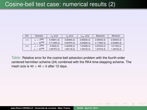
CFL Direction L1 error L2 error L∞ error Maximum Minimum
1.0 α = 0deg 5.43601(-2) 3.26394(-2) 2.65404(-2) 2.50503(-2) -2.65404(-2)α = 45deg 5.11205(-2) 2.93375(-2) 2.24284(-2) 2.11063(-2) -2.24284(-2)
0.5 α = 0deg 4.0020(-2) 2.25259(-2) 1.91928(-2) 2.87524(-2) 1.91193(-2)α = 45deg 3.45757(-2) 1.86116(-2) 1.43016(-2) 1.27016(-2) -1.43016(-2)
Table: Relative error for the cosine-bell advection problem with the fourth-ordercentered hermitian scheme (24) combined with the RK4 time-stepping scheme. Themesh size is 40× 40× 6 after 12 days.
Jean-Pierre CROISILLE - Universite de Lorraine - Metz, France NCAR - April 27, 2012
Cosine-bell test case: numerical results (3)
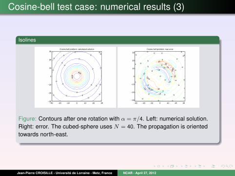
Isolines
0
0
0
0
00
0
00
00
0
0
0 0
0
0
00
0
0
0
0
800
800
Cosine bell problem: calculated solution
−30 −20 −10 0 10 20 30−30
−20
−10
0
10
20
30
−20−10
−10
−10
−10
−10−10
−10
0
0
0
0
0
0
00
0
0
0
0
0
0
0
0
0
0
0
0
0 0
0
0
0
0
0
0
00
0
00
00
10
10
1010
10
10
10
2020
Cosine bell problem: max error
−30 −20 −10 0 10 20 30
−30
−20
−10
0
10
20
30
Figure: Contours after one rotation with α = π/4. Left: numerical solution.Right: error. The cubed-sphere uses N = 40. The propagation is orientedtowards north-east.
Jean-Pierre CROISILLE - Universite de Lorraine - Metz, France NCAR - April 27, 2012
Compact Laplacian on the cubed-sphere
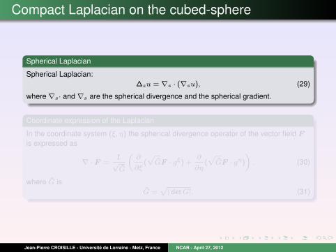
Spherical Laplacian
Spherical Laplacian:∆su = ∇s · (∇su), (29)
where ∇s· and ∇s are the spherical divergence and the spherical gradient.
Coordinate expression of the Laplacian
In the coordinate system (ξ, η) the spherical divergence operator of the vector field F
is expressed as
∇ · F =1√
G
„∂
∂ξ(p
GF · gξ) +∂
∂η(p
GF · gη)
«. (30)
where G isG =
p| det G|. (31)
Jean-Pierre CROISILLE - Universite de Lorraine - Metz, France NCAR - April 27, 2012
Compact Laplacian on the cubed-sphere
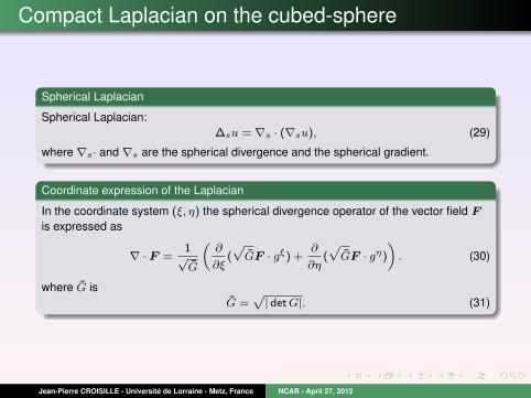
Spherical Laplacian
Spherical Laplacian:∆su = ∇s · (∇su), (29)
where ∇s· and ∇s are the spherical divergence and the spherical gradient.
Coordinate expression of the Laplacian
In the coordinate system (ξ, η) the spherical divergence operator of the vector field F
is expressed as
∇ · F =1√
G
„∂
∂ξ(p
GF · gξ) +∂
∂η(p
GF · gη)
«. (30)
where G isG =
p| det G|. (31)
Jean-Pierre CROISILLE - Universite de Lorraine - Metz, France NCAR - April 27, 2012
Laplacian on the cubed-sphere (2)
Compact Laplacian on each patch
From the gradient ∇su, we deduce on each patch the grid functions u1(ξ, η) andu2(ξ, η),
u1(ξ, η) =p
G∇su · gξ, u2(ξ, η) =p
G∇su · gη (32)
Using the discrete gradient above an approximation of the two functions u1 and u2 oneach patch is
(u1,h)ki,j =
pG“∇s,huk
i,j
”· gξ
i,j , (u2,h)ki,j =
pG“∇s,huk
i,j
”· gη
i,j . (33)
for −M ≤ i, j ≤ M and I ≤ k ≤ V I.
Jean-Pierre CROISILLE - Universite de Lorraine - Metz, France NCAR - April 27, 2012
Laplacian on the cubed-sphere (3)
Boundary conditions
Here there is no use of periodicity around great circles. Instead the discrete hermitianLaplacian is coordinate dependent. Thus we need boundary conditions along the fouredges of each patch to define local hermitian derivatives. We adopt the one-sidedapproximate derivative
u′(x) = δ+x uj −
1
2(δ+
x )2uj +1
3(δ+
x )3uj −1
4(δ+
x )4uj + O(h4), (34)
where the forward difference operator δ+x is
δ+x uj =
uj+1 − uj
h. (35)
The fourth-order approximate derivative is
ux,i =1
12h(−25ui + 48ui+1 − 36ui+2 + 16ui+3 − 3ui+4) (36)
Jean-Pierre CROISILLE - Universite de Lorraine - Metz, France NCAR - April 27, 2012
Laplacian on the cubed-sphere (4)
Discrete hermitian Laplacian
The discrete Laplacian is
∆huki,j =
1√
G
“(u1,h)k
ξ,i,j + (u2,h)kη,i,j
”. (37)
This is a formula dependent on the coordinate system (ξ, η) on each patch.
Jean-Pierre CROISILLE - Universite de Lorraine - Metz, France NCAR - April 27, 2012
Numerical test for the Laplacian
Spherical harmonics
The spherical harmonic with index (n, m), −n ≤ m ≤ n, 0 ≤ n is defined in sphericalcoordinates (θ, λ) by
fmn (x) = P
|m|n (sin θ)eimλ. (38)
The function P|m|n (z) is the associated Legendre polynomial of order n, m with
standard normalization given by Z 1
−1P|m|n (x)2dx = 1. (39)
Main property: the spherical harmonics are the eigenfunctions of the sphericalLaplacian.
Jean-Pierre CROISILLE - Universite de Lorraine - Metz, France NCAR - April 27, 2012
Numerical test for the Laplacian (2)
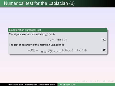
Eigenfunction numerical test
The eigenvalue associated with fmn (x) is
λn = −n(n + 1). (40)
The test of accuracy of the hermitian Laplacian is
e(fnm) = max
−M≤i,j≤M,I≤k≤V I|`∆h,sfn
m − λnfnm
´|, (41)
Jean-Pierre CROISILLE - Universite de Lorraine - Metz, France NCAR - April 27, 2012
Numerical results
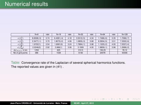
N=8 rate N=16 rate N=32 rate N=64 rate N=128
e(f11 ) 8.6508(-3) 3.74 6.4381(-4) 4.18 3.5512(-5) 4.34 1.7496(-6) 3.35 1.7066(-7)
e(f23 ) 2.3477(-1) 3.70 1.8073(-2) 4.06 1.0805(-3) 3.68 8.3954(-5) 3.51 7.3302(-6)
e(f48 ) 1.9702(1) 3.54 1.6991(0) 3.24 1.7884(-1) 3.98 1.1325(-2) 4.00 7.0537(-4)
e(f914) 2.0246(2) 2.92 2.666(1) 3.06 3.1909 4.00 1.9809(-1) 3.96 1.2696(-2)
∆ξmax in km 1250 625 312.5 156.25 78.12Nb of grid points 386 1538 6146 24578 93306
Table: Convergence rate of the Laplacian of several spherical harmonics functions.The reported values are given in (41) .
Jean-Pierre CROISILLE - Universite de Lorraine - Metz, France NCAR - April 27, 2012
Conclusion
Interest of the great circles approach
Uniformly high-order treatment of the sphere.
Avoids complex boundary treatment (ghost points, etc) at the inter patchboundaries.
High-order accuracy relies on purely one-dimensional periodic computations.
Only a (large) series of one-dimensional periodic “tridiagonal” systems to solve.
Implementation so far
Code in matlab so far.
Fourth-order Hermitian gradient is implemented.
Simple test-cases (linear advection) are tractable for N = 40.
Jean-Pierre CROISILLE - Universite de Lorraine - Metz, France NCAR - April 27, 2012
Ongoing work
Compact hermitian operators
Intrinsic design of higher-order differential operators such as spherical Laplacian,divergence or Biharmonic using great circles methodology.
No inter-patch boundary treatment depending of the differential operators to beapproximated.
Higher-order accuracy easy to obtain using very high-order hermitian derivatives(6-th order, 8-th order or higher.)
Implementation of the Laplace Tidal Equations.
MUSCL finite-volume schemes
High-order gradients are important for a stable, accurate MUSCL finite-volumemethod.
Various settings for the MUSCL are possible: cell-center or vertex-center.
Jean-Pierre CROISILLE - Universite de Lorraine - Metz, France NCAR - April 27, 2012

Some perspectives
Models
Investigation of complex linear wave problems on the sphere (atmosphere andocean).
Numerical computation of eigenmodes of linear operators of interest inclimatology/oceanography.
Scientific computing
Essential issue in climatology: local grid refinement on the cubed-sphere.
Parallel implementation of the great circles approach seems attractive.
Numerical analysis
Prove some convergence results of the great circles approach to compute thespherical gradient.
Jean-Pierre CROISILLE - Universite de Lorraine - Metz, France NCAR - April 27, 2012