finite-volume transport on various cubed-sphere grids · regarding grid uniformity, although far...

Available online at www.sciencedirect.com

Journal of Computational Physics 227 (2007) 55–78

www.elsevier.com/locate/jcp

Finite-volume transport on various cubed-sphere grids

William M. Putman a,*, Shian-Jiann Lin b

a NASA – GSFC Software Integration and Visualization Office – SIVO, Mail Stop 610.3, Greenbelt, MD 20771, United Statesb NOAA Geophysical Fluid Dynamics Laboratory, 201 Forrestal Road, Princeton, NJ 08540-6649, United States

Received 19 December 2006; received in revised form 6 July 2007; accepted 11 July 2007Available online 7 August 2007

Abstract

The performance of a multidimensional finite-volume transport scheme is evaluated on the cubed-sphere geometry.Advection tests with prescribed winds are used to evaluate a variety of cubed-sphere projections and grid modificationsincluding the gnomonic and conformal mappings, as well as two numerically generated grids by an elliptic solver and springdynamics. We explore the impact of grid non-orthogonality on advection tests over the corner singularities of the cubed-sphere grids, using some variations of the transport scheme, including the piecewise parabolic method with alternativemonotonicity constraints. The advection tests revealed comparable or better accuracy to those of the original latitudi-nal–longitudinal grid implementation. It is found that slight deviations from orthogonality on the modified cubed-sphere(quasi-orthogonal) grids do not negatively impact the accuracy. In fact, the more uniform version of the quasi-orthogonalcubed-sphere grids provided better overall accuracy than the most orthogonal (and therefore, much less uniform) confor-mal grid. It is also shown that a simple non-orthogonal extension to the transport equation enables the use of the highlynon-orthogonal and computationally more efficient gnomonic grid with acceptable accuracy.Published by Elsevier Inc.

Keywords: Cubed-sphere; Finite-volume; Advection; Transport schemes; Monotonicity

1. Introduction

The finite-volume dynamical core (FV core hereafter; [1]) has been generalized for quasi-uniform cubed-sphere grids in general non-orthogonal curvilinear coordinates using the National Oceanic and AtmosphericAdministration (NOAA) Geophysical Fluid Dynamics Laboratory’s (GFDL) Flexible Modeling System(FMS), with the final goal of being a shared modular component within various global modeling efforts.The original FV core ([1]; L04 hereafter) on the latitudinal–longitudinal grid is already an integral componentwithin the National Aeronautics and Space Administration (NASA) Goddard Earth Observing System(GEOS) modeling suite (e.g. [2–4]), the climate modeling efforts at NOAA/GFDL [5], and the CommunityAtmosphere Model at the National Center for Atmospheric Research (NCAR) [6,7]. The main objectives of

0021-9991/$ - see front matter Published by Elsevier Inc.

doi:10.1016/j.jcp.2007.07.022

* Corresponding author. Tel.: +1 301 286 2599; fax: +1 301 286 1775.E-mail address: [email protected] (W.M. Putman).

mailto:[email protected]

56 W.M. Putman, S.-J. Lin / Journal of Computational Physics 227 (2007) 55–78

the cubed-sphere development are to avoid the numerical difficulties of the spherical poles, explore a new levelof parallelism (two-dimensional X–Y domain decomposition) that is not practical within the current latitude–longitude grid construct [8], and to facilitate the development of a unified regional–global modeling system forboth weather and climate applications. In addition, the cubed-sphere geometry is ideally suited for adaptivemesh refinement [9–11], which could be effectively used for tropical cyclone predictions and simulations.

The cubed-sphere grid is a projection of a cube onto the surface of a sphere represented as six adjoining gridfaces which seamlessly cover the whole globe [12–15]. The cubed-sphere thus provides a quasi-uniform reso-lution over the whole globe, which offers several significant computational advantages over the existing lati-tude–longitude grid implementation. In particular, the quasi-uniform nature of the cubed-sphere grideliminates the parallelization difficulties associated with the poles, allowing a far more efficient implementationof the horizontal 2D domain decomposition, a feature that will be required of a truly scalable ultra-highresolution global cloud-resolving model. Furthermore, the convergence of meridians near the poles on the lat-itude–longitude grid requires the ‘‘Flux-Form Semi-Lagrangian’’ (FFSL) extension for stability if a large-time-step is to be used ([16]; LR96 hereafter). Due to the extreme grid aspect ratio, the FFSL extension onthe latitude–longitude grid creates a difficult load balancing issue due to a much larger halo region in the zonaldirection near the poles. In the full primitive-equation implementation, a polar filter is also required to stabi-lize the high frequency gravity waves that are being over-resolved at high latitudes. The pole-less and quasi-uniform nature of the cubed-sphere grid eliminates all of these issues.

For atmospheric modeling purposes, the cubed-sphere is not to be regarded as the perfect solution for grid-ding the whole sphere, nor is any other known grid. But it is an excellent compromise when considering griduniformity, orthogonality, and ease of applying existing high-order finite-volume transport algorithms.Regarding grid uniformity, although far superior than the latitude–longitude grid, the cubed-sphere is notas uniform as the Geodesic grid (e.g. [17–19]). But it is relatively easier to apply higher order transport algo-rithms due to its logically rectangular construct. It is also more natural for the implementation of a self-con-sistent nesting or mesh refinement capability within a regional–global modeling framework.

The original cubed-sphere grids (the gnomonic grids) are highly non-orthogonal, which impacts the accu-racy of the multidimensional algorithm of LR96 used in the FV core. This is because the LR96 algorithm for-mally requires an orthogonal grid. To overcome the limitations on the use of the gnomonic grids, we haveextended the LR96 algorithm for implementation on a general non-orthogonal curvilinear coordinate system.Alternatively, the cube can be projected onto the sphere to produce highly orthogonal conformal mappings[14]. We note, however, the conformal mapping is only orthogonal in the interior, with coordinate lines stillintersecting at the 8 corners at a 120-degree angle. Therefore, some modifications to the algorithm still need tobe made to counter the non-orthogonality near the corners. It would then seem advantageous to further relaxthe orthogonality requirement in order to allow for more uniformity, which not only enables a larger time-step, but potentially better overall accuracy.

Starting from the highly non-orthogonal gnomonic grids, one can trade some grid uniformity for improvedorthogonality by various numerical grid generation techniques. One of the objectives of this paper is to studythe best compromise between grid uniformity and orthogonality for the overall better accuracy and compu-tational efficiency (size of allowable time-step) versus the extension of the LR96 algorithm on the non-orthog-onal gnomonic grids.

We investigate modifications to the original gnomonic mappings of [12] by the elliptic solver grid generators(e.g. [20]) and the spring dynamics technique (e.g. [21]) to produce quasi-orthogonal mappings which preserveuniformity to a greater degree than the conformal mappings. The extent to which the improved orthogonalityof the numerically modified grids improves accuracy over the original gnomonic mappings will be evaluatedthrough standard two-dimensional advection test cases.

The organization of this paper is as follows. In Section 2, a modified form of the LR96 transport algorithmfor the general non-orthogonal curvilinear coordinate on the sphere is presented. In Section 3, the gnomonicgrid, the conformal grid, and the two numerically generated grids, the elliptic grid and the spring dynamicsgrid are inter-compared. We study, in Section 4, the sensitivity of the generalized LR96 flux-form transportscheme on the various cubed-sphere grids via a standard solid body rotation test case. The generalizedLR96 algorithm is further explored on the gnomonic grid through a deformational flow experiment and arecently introduced moving vortices experiment. Summary and conclusions are provided in Section 5.

W.M. Putman, S.-J. Lin / Journal of Computational Physics 227 (2007) 55–78 57

2. The multidimensional flux-form transport scheme on the general curvilinear coordinate system

The continuous differential form of the conservation law for a density-like field q in a general 2D curvilinearcoordinate system ðx; yÞ is

oqotþr � ðV!� qÞ ¼ 0 ð1Þ

where V!

is the horizontal vector velocity. Following L04, the finite-volume mean of the continuous q field isdefined as ~q

~qðtÞ � 1

DA

Z Zqðt; x; yÞdxdy ð2Þ

where the surface (double) integral covers the finite-volume under consideration, and DA ¼R R

dxdy is thearea of that finite-volume. Utilizing the divergence theorem, (1) can be integrated analytically in time (fromtime-step ‘‘n’’ to ‘‘n + 1’’) and in space (for the finite-volume):

~qnþ1 ¼ ~qn � 1

DA

Z tþDt

t

Iqðt; x; yÞ~V �~ndl

� �dt ð3Þ

where n! is the normal outward vector and dl is the elemental length along the cell wall. The contour integral(around the finite-volume) in (3) can be approximated by decomposing the flux integral into two 1D compo-nents using 1D flux-form operators along the two independent coordinate directions. The 1D operators rep-resent updates for one time-step to the predicted field due to the transport process from the two independentspatial directions ðx; yÞ. Defining ð~u;~vÞ as the contra-variant and ðu; vÞ as the covariant components of the vec-tor wind

V!¼ ~ue1

!þ ~ve2! ð4Þ

u ¼ V!� e1!; v ¼ V

!� e2! ð5Þ

and ð eu� ; ev�Þ as the corresponding time-averaged (from t to t + Dt), where ðe1!; e2!Þ are the local unit vectors of

the curvilinear coordinate system, the 1D finite-volume flux-form operator F in the x-direction can be writtenas

F ð eu� ;Dt; ~qnÞ ¼ � DtDA

dx½vDy sinðaÞ� ð6Þ

¼ � DtDA

dx½ eu�q�ð eu� ;Dt; ~qnÞDy sinðaÞ� ð7Þ

where v is the time-averaged mass flux across the cell wall

v ¼ 1

Dt

Z tþDt

tq~udt � eu�q�ð eu� ;Dt; ~qnÞ ð8Þ

In the above derivation, q* is interpreted as the time mean density value of all material passing through thecell edge from the upwind direction:

q�ð eu� ;Dt; ~qnÞ � 1

Dt

Z tþDt

tqdt ð9Þ

and the following definitions are used: Dy the local curvilinear grid length along the cell edge in the y-direction,a the ‘‘angle’’ between the two local unit vectors ðe1

!; e2!Þ of the curvilinear coordinate system

cosðaÞ ¼ e1!� e2! ð10Þ

and the difference operator is defined as

dxq ¼ q xþ Dx2

� �� q x� Dx

2

� �ð11Þ


Similarly, the 1D flux-form operator in the y-direction, G, can be written as

Gð ev� ;Dt; ~qnÞ ¼ � DtDA

dy ½Y Dx sinðaÞ� ð12Þ

¼ � DtDA

dy ½ ev�q�ð ev� ;Dt; ~qnÞDx sinðaÞ� ð13Þ

Note, in (7) and (13), the local metric factor due to grid non-orthogonality, sin(a), which originated fromthe inner vector product in (3), reduces to unity for orthogonal grids. Following LR96, to achieve higher orderaccuracy, the 1D flux-form operators are applied in a directionally symmetric fashion by averaging two anti-symmetrical schemes, formally resulting in the use of four 1D flux-form operators (for two-dimensionalschemes). To avoid the flow deformation induced directional splitting error, the ‘‘inner operators’’ arereplaced by their 1D advective-form counterparts (f and g, in the x- and y-directions, respectively). Definingthe following short hand notation:

qx ¼ ~qn þ 1

2f ½ eu� ;Dt; ~qn� ð14Þ

qy ¼ ~qn þ 1

2g½ ev� ;Dt; ~qn� ð15Þ

The 2D transport algorithm can be written as

~qnþ1 ¼ ~qn þ F ½ eu� ;Dt; qy � þ G½ ev� ;Dt; qx� ð16Þ
In principle, the inner operators can be different schemes and/or having lower order accuracy than the
‘‘outer’’ flux-form operators. For economical reason, one may choose a lower order scheme for the inner oper-ator. However, it was found, on modern parallel computers with substantial inter-processor communicationrequirement, using the same higher order schemes (e.g. PPM vs. the second-order van Leer scheme) as ‘‘inner’’operators improved the accuracy with only minimal additional computational cost. L04 derived the inner‘‘advective-form’’ operators used in (14) and (15) using the same flux-form operators with an explicit diver-gence correction term (see Eqs. (7) and (8) in L04). To better preserve the monotonicity within the samenumerical framework as in L04, the divergence correction term can be made time implicit (with no additionalcost) as follows:

qx ¼ 1

2~qn þ ~qn þ F

1þ F ðq� ¼ 1Þ

� �ð17Þ

qy ¼ 1

2~qn þ ~qn þ G

1þ Gðq� ¼ 1Þ

� �ð18Þ

where

F ðq� ¼ 1Þ ¼ � DtDA

dx½ eu�Dy sinðaÞ�

and

Gðq� ¼ 1Þ ¼ � DtDA

dy ½ ev�Dx sinðaÞ�

Eq. (16) together with (17) and (18) form the general 2D transport scheme that will be evaluated in subse-quent sections. Practically any 1D forward-in-time finite-volume scheme can be used. LR96 and L04 arguedthat the PPM scheme achieves an excellent balance between accuracy and computational efficiency, and assuch is our method of choice for the 1D operators. The use of the same inner and outer operator withinthe LR96 algorithm also avoided a potential stability issue [22]. Alternative monotonicity constraints forlarge-time-step has been studied in [23].

In Section 4, the performance of several schemes for determining the subgrid distributions on the cubed-sphere are investigated. These include, (i) the optimized PPM operator used within the latitude–longitudeFV core, labeled as ORD = 4 (see B3 and B4 in L04), (ii) a quasi-monotonic scheme, using the base PPM with


Huynh’s second constraint [24] is labeled as ORD = 5, (iii) a non-monotonic quasi-fifth-order scheme, labeledas ORD = 6 (described in full details in Appendix B), and, (iv) an extension of the ORD = 5 scheme with spe-cial treatment of edge discontinuities on the cubed-sphere grid labeled as ORD = 7 (describe in details inAppendix C).

3. The cubed-sphere grids

In our implementation, the cubed-sphere grid geometry is completely defined by the locations of the vertices(of the finite-volumes). The cell areas ðDAÞ, grid lengths in the two cartesian directions ðDx;DyÞ, and a non-orthogonal metric factor (sina), where a is the angle formed at the intersection of the coordinates connectingthe finite-volume vertices, are derived quantities. The cell vertices can be generated in several ways: the originalgnomonic mapping based on the equidistant [12] or equiangular projections [13], the highly orthogonal con-formal mapping [14], or numerical modifications to these analytical mappings by an elliptic solver (see [25] fordetails) or the spring dynamics generator [21]. Grid resolutions are defined in this paper as cM where M rep-resents the number of grid cells along each of the edges of a cubed-sphere face thus the total number of cellsfor a given resolution is M · M · 6.

Cell areas ðDAÞ are computed by the spherical excess formula (Eq. (19) as in [26]) given the 4-sided spher-ical quadrilateral for each finite-volume with internal angles ða1; a2; a3; a4Þ and the radius of the sphere R

DA ¼ R2½a1 þ a2 þ a3 þ a4 � 2p� ð19Þ
The cell edges for all grids are prescribed to be great circle arcs and thus this formula for the cell area is
exact and only degenerates on a perfectly orthogonal grid where [a1 + a2 + a3 + a4 � 2p] = 0. The grid lengthsðDx;DyÞ are thus computed by great circle distances. Given the latitude–longitude coordinate of two points onthe sphere ðk1; h1Þ and ðk2; h2Þ the great circle distance dh can be computed as

dh ¼ R cos�1½cos h1 cos h2 cosðk1 � k2Þ þ sin h1 sin h2� ð20Þ
An alternative form, which is less sensitive to rounding errors for small angles can be used based on the
angle s between two vectors ~V 1; ~V 2 connecting from the center of the sphere to the two points

~V i ¼ R cos hi cos ki; cos hi sin ki; sin hið Þ ð21Þ

s ¼ cos�1~V 1 � ~V 2

R2

!ð22Þ

dh ¼ sins2

� �¼ 2 arcsin

ffiffiffiffiffiffiffiffiffiffiffiffiffiffiffiffiffiffiffiffiffiffiffiffiffiffiffiffiffiffiffiffiffiffiffiffiffiffiffiffiffiffiffiffiffiffiffiffiffiffiffiffiffiffiffiffiffiffiffiffiffiffiffiffiffiffiffiffiffiffiffiffiffiffiffiffiffiffiffiffiffiffiffiffiffiffiffiffiffiffisin2 h2 � h1

2

� �þ cos h1 cos h2 sin2 k2 � k1

2

� �s !ð23Þ

3.1. Gnomonic projection

The gnomonic mapping of the cubed-sphere is obtained by inscribing a cube within a sphere and expandingto the surface of the sphere [14]. A local cartesian coordinate system is determined for each of the six faces ofthe cube, and a transformation is applied to connect each point on the cube to the spherical surface. There aretwo choices for the local coordinates on the faces of the cube. The mapping between local coordinates ðx; yÞf ,ranging from ½�a;þa� for cube faces f 2 1, 6 where a ¼

ffiffi3p

3R and spherical coordinates ðX ; Y ; ZÞ for the local

face centered in the �Y direction with an equidistant gnomonic mapping on a sphere of radius R takes theform

ðX ; Y ; ZÞ ¼ Rrðx;�a; yÞ

r ¼ffiffiffiffiffiffiffiffiffiffiffiffiffiffiffiffiffiffiffiffiffiffiffiffia2 þ x2 þ y2

p:

Alternatively, a gnomonic mapping can be defined based on an equiangular projection where local coordi-nates are defined as

Fig. 1.one co(d) the


x ¼ a tan x0

y ¼ a tan y0

where the coordinates ðx0; y0Þ range from ð�p=4;þp=4Þ. The equiangular projection at 2-degree resolution isdisplayed in Fig. 1c. The equiangular projection leads to a more uniform distribution of grid cells on the spherethan the equidistant projection and an ideal scaling of the minimum grid length with increasing resolution(Fig. 2). Either choice of gnomonic projection produces a cubed-sphere mapping which is highly non-orthog-onal and non-conformal. A conformal mapping is one in which the angles are preserved between intersectingsmooth curves [14]. The gnomonic mapping produces a sharp angular discontinuity across the edges of the cubefaces. The conformal mapping maintains a smooth transition across these edges and produces the optimalorthogonality for the cubed-sphere grid.

The cubed-sphere grids at 2� (c44) resolution displaying cells on the sphere, the image focuses on the distribution of grid cells nearrner of the grid; (a) conformal mapping, (b) the gnomonic grid modified by elliptic solver, (c) equiangular gnomonic mapping andgnomonic grid modified by spring dynamics.

Scaling of the Shortest Grid Lengthfor Various Cubed-Sphere Grids

0.0001

0.001

0.01

0.1

1

1 10 100 1000

Number of Cells on Tile Edge

Min

Dx

/ [2

* A

TA

N(1

/SQ

RT

(2))

]Gnomonic Conformal Elliptic Solver 4/3 Scaling

Fig. 2. Scaling of the minimum grid length with increasing resolution for the gnomonic, conformal and elliptic cubed-sphere gridmappings.


3.2. Conformal projection

A conformal projection preserves the angles between intersecting curves on adjoining faces of the cubed-sphere and is differentiable to any order at all points except the eight singularities. The conformal mappingis obtained as described in [14] via a reversible sequence of transformations between a plane and the sphereusing a stereographic projection and a Taylor series to complete the transformation from the intermediate ste-reographic plane. The conformal projection (Fig. 1a) produces a grid with exceptional orthogonality traits and

a near uniform aspect ratio DxDy ¼ 1� �

throughout the sphere. The corner singularities remain non-orthogonal

with angular deviation from 90� fixed at 30�, the vertices surrounding the corner also remain slightlynon-orthogonal with the first grid point off the corner maintaining a deviation from orthogonality near8.5� regardless of grid resolution. The strict orthogonality constraints on the conformal mapping lead to aconvergence of grid cells near the eight singularities of the grid. While this convergence is far less severe thanthat of the latitude–longitude grid at the spherical poles, the scaling of minimum grid length with resolution isfar from ideal. Stretching factors can be used to rescale the conformal mapping [26], or elliptic solvers orspring dynamics techniques may be applied to reduce this convergence near the corners while maintainingstrong orthogonality constraints. Stretching does not compromise the conformal attributes of the grid, northe superior orthogonality traits of the conformal mapping. However, stretching leads to severe aspect ratiodistortion along the edges of each face as resolution increases, distortion so severe that it prevents effectivestretching of the conformal mapping for producing efficient high resolution grids.

3.3. Elliptic solvers

Elliptic grid generation is the iterative relaxation of a first-guess grid (via successive over-relaxation) to sat-isfy a quasi-linear elliptic system of partial differential equations (PDEs) while imposing smoothness andorthogonality constraints [20]. In the case of the cubed-sphere, the initial grid is the original equiangular


gnomonic projection of the cubed-sphere. Each face of the physical grid in spherical coordinates is mapped toa two-dimensional u-v parametric space (scaled from 0 to 1 in the X–Y direction). The elliptic solver solves thesystem of PDEs in parametric space while imposing the desired physical constraints; orthogonality and uni-form grid spacing are the most important constraints for this application. The symmetry of the cubed-spherecan be exploited to reduce the number of points that actually need to be run through the elliptic solver; cal-culations can be performed on 1

8-th of a single face and the solution can be mapped symmetrically to the rest of

the cubed-sphere.There are two options for imposing orthogonality constraints: the Neumann constraint that allows the grid

points to slide along the boundary of each face, and the Dirichlet constraint that holds the edge points fixedwhile adjusting the interior points and maintaining a quasi-uniform grid cell spacing. The Neumann approachcomputes a shift for each grid point along the boundary of the grid by forcing the dot product of u Æ v to beequal to zero; this approach will produce a convergence of grid cells near the corners. To limit this conver-gence, a weighting function can be applied to the first n grid points off the corner along each boundary ofthe grid (Eq. (24)). The weight, rwgt, and n become tunable parameters to enforce a significant amount ofdependence on the orthogonality constraint while limiting the minimum grid length at the corners by thedesired amount (this implementation limits convergence to grid lengths to 60% of the representative resolu-tion or greater.) The rwgt ranges from 0.0 to 1.0, with typical values between 0.7 and 1.0

wt ¼MIN 1:0; LOGi

n

� �rwgt 1:0� inð Þ !

ð24Þ

Orthogonality may also be imposed through the use of orthogonal control functions, the Dirichletapproach. These functions are evaluated at the boundary to impose orthogonality, while maintaining the ori-ginal grid spacing along the boundaries. Transfinite interpolation is applied to interpolate the control func-tions from the boundary to the interior of the grid. In addition, a blending function can be applied toforce the interior points to remain close to the original grid spacing. The blended control function can be usedto impose orthogonality and smoothing constraints within the elliptic solver.

A combination of these techniques allows the boundary points to slide a little to force orthogonality withthe Neumann constraint while blending uniformity and orthogonality functions throughout the domain withthe Dirichlet constraint. This leads to the quasi-orthogonal elliptic cubed-sphere grid with constraints onorthogonality while maintaining a reasonable minimum to maximum grid cell length ratio. The elliptic solveris initially run to convergence with the Neumann constraint and a given weight (rwgt) which varies with res-olution to limit convergence to 0.6 of the representative resolution. Typical weights for each resolution aredetermined via experimentation to be (1.00, 0.925, 0.875, 0.800, and 0.775 for the resolutions 4� (c22), 2� (c44),1� (c90), 0.5� (c180), and 0.25� (c360) respectively with a value of n = 0.25 * npts). The resulting grid is thenrun to convergence with a smoothed Dirichlet constraint to enforce orthogonality/uniformity throughout theremainder of the grid while keeping the edge lengths fixed. The result is a set of cubed-sphere grids (a c44example is presented in Fig. 1b) with smoothly varying coordinate lines at cell edges and mean orthogonalitysimilar to the conformal grid, while restricting quasi-orthogonality to the immediate vicinity of the singular-ities. As resolution increases, the aspect ratio grows along the edges of each face due to a stretching of gridlines away from the face edges, however the maximum grid length remains much less 2 times the represen-tative resolution.

3.4. Spring dynamics

The spring dynamics modifications [21] to the cubed-sphere are formulated on a 3D cartesian coordinatesystem. Two types of springs are used; the compression type and the torsion type (our modification to thespring dynamics technique). The compression springs mostly made the grid more spatially uniform whereasthe torsion springs are for enforcing orthogonality by nudging the vertices in the direction that reduces thelocal deviation from orthogonality. With the spring dynamics generator, one can tune the strength of thesprings to obtain grids that are (i) more orthogonal, (ii) more uniform, (iii) have a larger minimum grid length(to allow larger time-step), or (iv) a compromise of the above. The spring tensions can be tuned to produce

Table 1Grid length (in kilometers) characteristics for the conformal, elliptic and spring cubed-sphere grids for increasing resolution from 4� (c44)to 0.25� (c360)

Resolution Conformal Elliptic Spring

Min Max Min/Mean Min Max Min/Mean Min Max Min/Mean

c22 166 471 0.43 281 522 0.67 262 567 0.63c44 66 235 0.33 140 288 0.67 134 289 0.64c90 25 115 0.26 69 152 0.67 59 149 0.57c180 10 58 0.20 33 80 0.63 29 73 0.57c360 4 29 0.16 15 44 0.60 – – –


quasi-orthogonal mappings in a similar way as the Neumann and Dirichlet constraints in the elliptic solver.Grids generated by the spring dynamics (a c44 example is presented in Fig. 1d) tend to have smoother solu-tions and fewer numerical artifacts than the elliptic solver grids. However, both techniques suffer from slowconvergence rates (for the generation), especially at fine resolutions c360 and finer. However for typical globalclimate/weather applications this is a one-time procedure for a given resolution. Numerically modified grids(such as the spring and elliptic grids) are not ideal for adaptive mesh refinement applications since refinementsto the grid would require further iterations and is thus not suitable for dynamic refinement. The gnomonicgrids, particularly at high resolutions, would seem to be ideal from the mesh refinement perspective.

3.5. Grid characteristics summary

We examine the characteristics of the gnomonic, conformal, elliptic and spring grids with an emphasis onminimum grid length, orthogonality, and uniformity. Sample grids of the conformal mapping, modified ellip-tic, and spring-dynamics grids are presented in Fig. 1. The minimum grid length for the conformal grid reducesdramatically with increasing resolution, making the conformal mapping an inefficient choice for high resolu-tion global modeling. The grids modified by the elliptic solver or spring dynamics have been tuned to over-come this convergence problem (Table 1) by limiting the convergence to between 0.5 and 0.6 ratio ofshortest to mean grid lengths. Closer examination of the convergence of the minimum grid length with increas-ing resolution (Fig. 2) reveals that the elliptic grids are converging at a much slower rate than the conformalmapping and on a similar slope to the ideal gnomonic mapping (this is also the case for the spring grids, notshown).

The numerically modified grids have also been tuned to prevent severe distortion in aspect ratio along faceedges (Table 3). The distribution of resolution across the sphere (uniformity, as represented by the cell area)remains unchanged for the conformal and elliptic grids, while slight variations exists in the spring grids. Slightnon-orthogonality is present in the immediate vicinity of the corners, even with the conformal mapping. Thenon-orthogonality converges with resolution for the conformal and elliptic grids as evidenced by the maxi-mum and mean angle deviation from orthogonality (Table 2). The spring dynamics are producing smoothgrids with efficient uniformity and minimum/maximum grid length characteristics, but are not producingthe most efficient grids in terms of orthogonality. With further tuning it is expected that the spring dynamicsmodified grids can produce orthogonality convergence characteristics similar to the elliptic grids.

Table 2As in Table 1 but for angle deviation from orthogonality


Max Mean Max Mean Max Mean

c22 8.52 1.13 13.87 1.89 9.36 0.99c44 8.53 0.65 12.79 1.13 11.97 0.84c90 8.53 0.34 11.97 0.69 10.93 0.51c180 8.53 0.17 11.64 0.43 14.20 0.52c360 8.53 0.09 11.43 0.24 – –

Table 3As in Table 1 but for aspect ratio (Dx:Dy)


Max Mean Max Mean Max Mean

c22 1.09 1.07 1.33 1.10 1.50 1.20c44 1.09 1.04 1.50 1.14 1.54 1.20c90 1.09 1.02 1.77 1.16 1.67 1.24c180 1.09 1.01 1.97 1.17 1.50 1.14c360 1.09 1.00 2.25 1.17 – –


4. Numerical experiments

The coordinates at the 12 interfaces between any two adjoining faces of the cubed-sphere are discontinuous,except the conformal grid where all edges are continuously differentiable excluding the eight corners. We eval-uated four different variations (ORD = 4–7) to subgrid piecewise parabolic reconstruction. Except theORD = 7 scheme, all schemes treated the interfaces as if they were continuous. The ORD = 4 scheme isthe optimized monotonic PPM described in L04, which behaves nearly the same as the original PPM exceptthat total operation count has been reduced. The ORD = 5 scheme is the same as ORD = 4 but with themonotonicity constraint replaced by Hunyh’s second constraint. The ORD = 6 scheme uses instead a fifth-order interpolation for obtaining the edge values that are left unlimited (Appendix B). The ORD = 7 scheme(Appendix C) is a further modification to ORD = 5 scheme with the face edges treated more accurately as dis-continuities. For all schemes tested on all grids, mass is conserved to machine precision. Three types of theprescribed advective winds are used: solid body rotation, deformational flow, and a combination of these pro-ducing moving vortices, as described below.

4.1. Solid body rotation of a cosine bell

The 2D advection test case of [27] (a solid body rotation of a cosine bell) is used to evaluate the transportalgorithm derived in Section 2 on the gnomonic, conformal, elliptic and spring cubed-sphere grids. The fol-lowing parameters for the radius of the earth (R), the rotation rate (X) and the acceleration due to gravity (g)

R ¼ 6:37122 106 m; X ¼ 7:292 10�5 s�1; g ¼ 9:80616 ms�2

are used for this test. The initial height field is a cosine hill given by

hðk; hÞ ¼h0

2

1þ cos pr

R0

� ��; if r < R0

0; if r P R0

(ð25Þ

where h0 = 1000 m, R0 = R/3 and r is the great circle distance between ðk; hÞ and the center, initially given atðkc; hcÞ ¼ 3p

2; 0

.

The wind components normal to the cell walls can be explicitly defined on the C-Grid by taking the deriv-ative of the prescribed streamfunction, Eq. (26)

w ¼ �Ru0ðsin h cos b� cos k cos hsinbÞ; ð26Þ

u ¼ � owoy; ð27Þ

v ¼ owox; ð28Þ

or computing directly in component form on a latitude–longitude orientation ðukh; vkhÞ using the analytic form,Eq. (29) and (30), as in [27] and re-orienting to the cubed-sphere geometry ðu; vÞ as in Appendix A

ukh ¼ u0ðcos h cos bþ sin h cos k sin bÞ ð29Þvkh ¼ �u0 sin k sin b ð30Þ

Fig. 3. Time traces of normalized l1, l2 and l1 errors for the cosine bell advection test with southeastward flow oriented over the corners ofthe cubed-sphere with the ORD = 4 advection scheme on multiple cubed-sphere grids at c90 (1�) resolution.



where b is the angle between the axis of solid body rotation and the polar axis of the spherical coordinate sys-tem, and u0 = (2pR)/(12 days). The corresponding contra-variant components are simply

Fig. 4.the cu

~u ¼ usinðaÞ ; ~v ¼ v

sinðaÞ ð31Þ

where a is the ‘‘local’’ angle of the coordinate system, (as defined by Eq. (10)). Solid body rotation experimentsreveal the choice of methods for defining the initial winds to be insignificant and all experiments herein usewinds defined in component form and re-oriented to the cubed-sphere geometry.

Time traces of normalized l1, l2 and l1 errors for the cosine bell advection test with southeastward flow oriented over the corners ofbed-sphere for the gnomonic mapping using advection schemes top) ORD = 5, middle) ORD = 6 and bottom) ORD = 7.

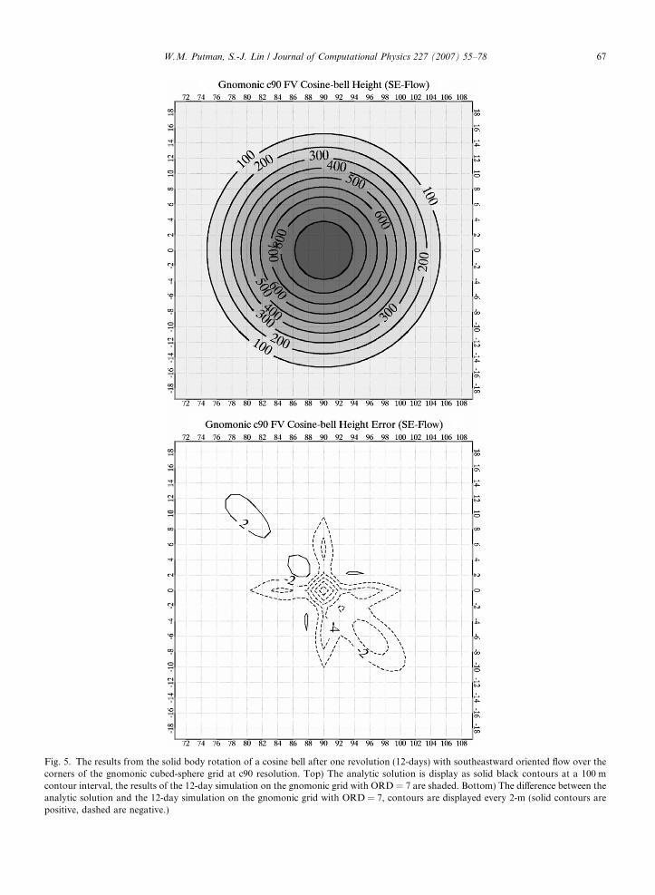
Fig. 5. The results from the solid body rotation of a cosine bell after one revolution (12-days) with southeastward oriented flow over thecorners of the gnomonic cubed-sphere grid at c90 resolution. Top) The analytic solution is display as solid black contours at a 100 mcontour interval, the results of the 12-day simulation on the gnomonic grid with ORD = 7 are shaded. Bottom) The difference between theanalytic solution and the 12-day simulation on the gnomonic grid with ORD = 7, contours are displayed every 2-m (solid contours arepositive, dashed are negative.)



4.2. Deformational flow

A deformational flow test in spherical geometry (a detailed description of this test is available in the follow-ing references [28–30]) is used to further evaluate the generalized FV advection scheme on the gnomoniccubed-sphere. This test is an idealized cyclogenesis problem where two steady vortices are generated, centeredover two corners of the cubed-sphere geometry in a rotated spherical coordinate system where the north pole islocated at ðk0; h0Þ ¼ ðp� 0:8; p=4:8Þ.

4.3. Moving vortices

The moving vortices experiment is an extension of the deformational flow test combined with a solid bodyrotation to form two moving vortices over the surface of the sphere (details can be found in [31].) The hori-zontal velocity components become time-dependent and are updated at every time-step based on the locationof the vortex centers along a pre-determined great-circle trajectory. In our case, the trajectory is chosen suchthat the vortex centers pass over four corners and along two edges of the cubed-sphere.

4.4. Results

We first evaluated the conformal, gnomonic, elliptic and spring grids at varying resolutions increasing fromc12 (8�) to c192 (0.5�) for the solid body rotation test case. While varying grid resolutions and flow orienta-tions were studied, results are presented for each scheme with southeasterly flow b ¼ p

4

oriented over four

corners and 2 face edges of the cubed-sphere at the c90 (1�) resolution. To maintain stability, the conformalgrid is tested with a time-step of 900 s, while all other grid types use a time-step of 1800 s. The standard l1, l2,and l1 normalized errors as in [27] are evaluated at each time-step throughout one full revolution of the cosinebell.

Gnomonic FV Convergence (Cosine-Bell : SE-flow)

1.0E-04

1.0E-03

1.0E-02

1.0E-01

1.0E+00

c12 c24 c48 c96 c192

Cubed-Sphere Resolution

Nor

mal

ized

Err

ors

l_infl_1l_2

Fig. 6. Convergence of normalized l1, l2 and l1 errors for the solid body rotation of a cosine bell test after one revolution (12-days) withsoutheastward oriented flow over the corners of the gnomonic cubed-sphere grid with the ORD = 7 advection scheme at resolutions ofc12, c24, c48, c96, and c192.


For the ORD = 4 scheme, time-traces of the normalized errors are presented in Fig. 3. The elliptic andspring grids produce the smallest errors as they have been tuned to obtain a compromise between orthogonal-ity, grid uniformity and smoothness. Even though the 12 face edges were naively treated as continuous, there isno evidence of spurious spikes in the standard errors as the cosine bell passes smoothly over the corners on thegrid and along the face edges exhibiting no signs of discontinuity. While the elliptic and spring grids do pro-duce the smallest errors, the gnomonic grid is slightly outperforming the conformal grid, and it is evident thatthe gnomonic grid provides sufficiently accurate results. Since it allows the largest possible time-step, all fur-ther tests presented in this paper will use the gnomonic grid projection.

Fig. 4 shows the time-traces of the normalized errors for the same cosine bell solid body rotation test on thegnomonic grid for the other three finite-volume subgrid distribution schemes (ORD = 5, ORD = 6, andORD = 7). The non-monotonic ORD = 6 scheme produces significantly smaller l1 errors, while the globalerrors are increased, relative to ORD = 5 and ORD = 7 schemes. The ORD = 5 and ORD = 7 schemes applyHunyh’s second constraint thus limiting the undershoots to near machine precision while the ORD = 6 is non-monotonic leading to much larger negative values (�10�3). With the ORD = 7 scheme, all errors are slightly

Table 4Normalized errors for the solid body rotation of a cosine bell on a c32 gnomonic cubed-sphere grid with southeasterly oriented flow for theORD = 4, ORD = 5, ORD = 6 and ORD = 7 advection schemes

Grid Scheme DT Min l1 l2 l1

Gnomonic FV ORD = 4 5400 3.369E�67 0.072 0.079 0.140Gnomonic FV ORD = 5 5400 �7.813E�26 0.048 0.045 0.072Gnomonic FV ORD = 6 5400 �1.271E�02 0.089 0.054 0.048Gnomonic FV ORD = 7 5400 1.308E�70 0.047 0.045 0.074

Fig. 7. The initial square block (heavy contour) and the final height field (shaded, values >15 – red, >35 – orange, >55 – yellow, >75 –green, >95 – blue) after one revolution (12-days) with southeastward oriented flow over the corners of the gnomonic cubed-sphere grid atc90 resolution with the ORD = 7 advection scheme. (For interpretation of the references to colour in this figure legend, the reader isreferred to the web version of this article.)


reduced with the special edge treatment at the 12 discontinuous interfaces of the cubed-sphere. Due to this andits monotonicity characteristics results presented from this point use exclusively the ORD = 7 scheme.

The spatial distribution of the height field after one 12-day revolution and the difference from the exactsolution is presented in Fig. 5. There is no clear distinction between the exact solution and the simulated heightfield (top panel). Bottom panel reveals the largest error (about 1% of the exact) to be centered at the peak ofthe cosine bell structure, which is due to the expected clipping effect from the monotonicity constraint.

The convergence of the ORD = 7 scheme is displayed for the solid body rotation test case (Fig. 6). Theseresults compare directly to Fig. 8b of [30] for the convergence of the discontinuous Galerkin (DG) scheme onthe cubed-sphere. Error levels with the FV scheme on the gnomonic cubed-sphere grid are consistent with thehigher order DG scheme. The FV convergence rates for the solid body rotation are 1.97, 2.54 and 2.68 for thel1, l2, and l1 errors respectively. Due to the more uniform cubed-sphere geometry and the improved inner

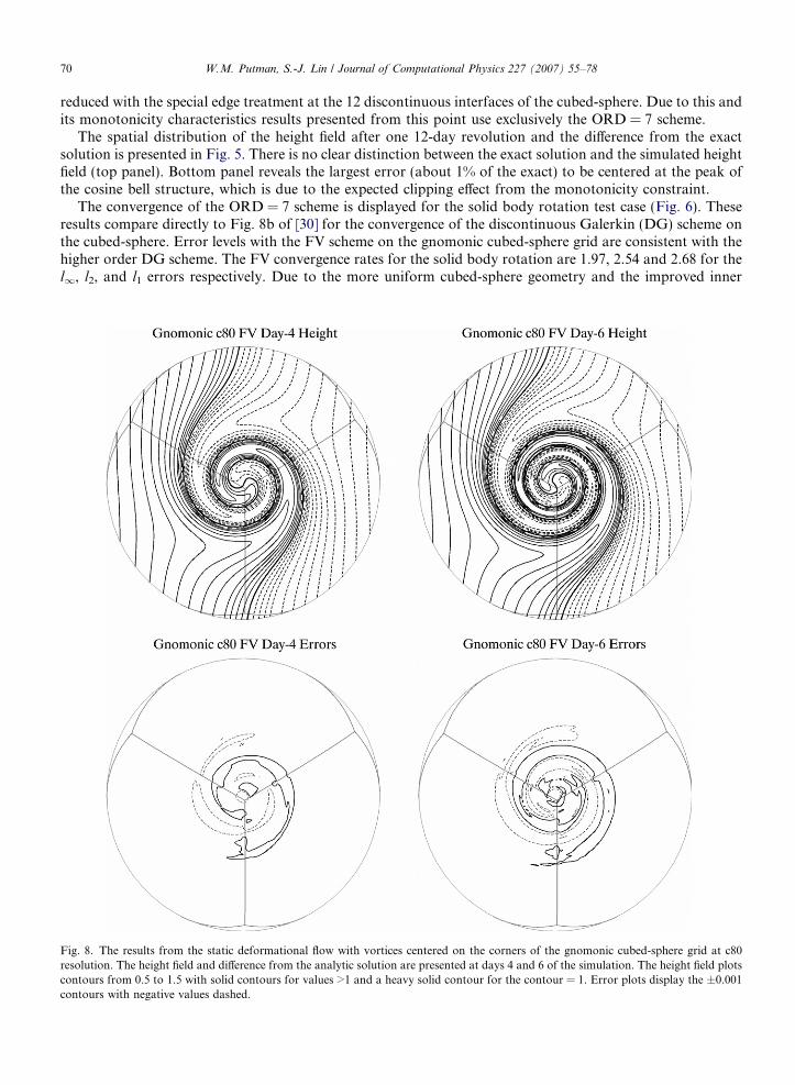
Fig. 8. The results from the static deformational flow with vortices centered on the corners of the gnomonic cubed-sphere grid at c80resolution. The height field and difference from the analytic solution are presented at days 4 and 6 of the simulation. The height field plotscontours from 0.5 to 1.5 with solid contours for values >1 and a heavy solid contour for the contour = 1. Error plots display the ±0.001contours with negative values dashed.


operators given by (17) and (18), these results are more accurate than the original LR96 algorithms on thelatitude–longitude grid at similar resolutions.

The results from each subgrid distribution scheme on the gnomonic grid are summarized in Table 4 at thec32 resolution, comparable to the 128 · 64 resolution used for the latitude–longitude grid in LR96 and theresults presented in Table 3 of [32] summarizing the results of various schemes (including the Semi-Lagrangianinherently conserving and efficient (SLICE), the cell-integrated Semi-Lagrangian (CISL), conservative cascadescheme (CCS) and a 2D forward-in-time upwind-biased flux-form scheme extended to the ‘reduced sphericalgrid’ (RG2.8)) for rotation over the spherical poles. The FV gnomonic cubed-sphere results for the l1 and l2errors for the ORD = 5 and ORD = 7 schemes over the corner singularities produce the smallest errors, betterthan any scheme presented with flow over the spherical poles, while the l1 errors are comparable to theSLICE, CISL, and FFSL-4/FFSL-5 schemes.

A similar test case to that of [27] is designed to demonstrate the shape-preserving nature of the monotonic-ity constraints within the finite-volume transport schemes. A square block with h0 = 100 m is advected overthe corners with the ORD = 7 scheme on the gnomonic c90 grid with a time-step of 1800 s. Fig. 7 displaysthe final height field after one full rotation over the corners. Overshoots and undershoots are clearly controlledby the monotonic constraint, as there are no significant negative values. The edges of the block are smoothed,however the peak value of the block is maintained and the general structure is preserved. Normalized errorsfor this case are l1 = 6.39e�1, l1 = 1.32e�1, and l2 = 1.99e�1.

Results from the deformational flow test on the c80 gnomonic cubed-sphere grid with the FV ORD = 7scheme and a 3600 s time-step are presented in Fig. 8. The top panels show the simulated vortices at days4 and 6, and the bottom panels display the difference from the exact solution. The vortices (simulated at dia-metrically opposite vertices on the cubed-sphere as in [30]) are well resolved and differences from the numericalsolution by day 6 are on the order of ±1e�3. Further, there are no noticeable impacts of discontinuities alongthe face edges, the errors reveal only a slight diffusion in the simulation as compared with the exact solution.

Gnomonic FV Convergence (Deformational Flow)

1.0E-06

1.0E-05

1.0E-04

1.0E-03

1.0E-02

1.0E-01

c12 c24 c48 c96 c192 c384 c768


Nor

mal

ized

Err

ors

l_infl_1l_2

Fig. 9. Convergence of normalized l1, l2 and l1 errors for the static deformational flow with vortices centered on the corners of thegnomonic cubed-sphere grid with the ORD = 7 advection scheme at resolutions ranging from c12 to c768.

Fig. 10. The results from the moving vortices test case with flow oriented over the corners of the gnomonic cubed-sphere grid at c80resolution. The height field is presented at days 6, 9 and 12 of the simulation. Contours range from 0.5 to 1.5 with solid contours for values>1 and a heavy solid contour for the contour = 1.



The convergence of the standard l1, l2, and l1 normalized errors at day-6 are presented in Fig. 9 and they com-pare favorably with results presented in [30] for the DG scheme on the cubed-sphere.

Results from the recently developed moving vortices test case of [31] are presented in Fig. 10 and the dif-ference from the exact solution is presented in Fig. 11. The flow of the solid body rotation aspect of this case isoriented southeasterly advecting the simulated vortices over four corners and two face edges of the c80 gno-monic cubed-sphere. The FV ORD = 7 scheme is used for this simulation with an 1800 s time-step. The vor-tices are again well resolved throughout the 12-day simulation, errors grow (isolated in the vicinity of thegenerated vortices) on the order of three percent of the value of the exact height field. The time-traces ofthe normalized l1, l2, and l1 errors are presented in Fig. 12 and can be compared directly to results presentedin Fig. 7 of [31] for the FV scheme on the latitude–longitude grid. While the l1 normalized error is slightlylarger than results presented in [31], the l1 and l2 errors produce comparable results and there is no evidenceof degradation in the simulation as the vortices pass over the corners and along face edges of the cubed-sphere.The convergence of the l1, l2, and l1 errors with increasing resolution from c48 (2�) to c768 (0.125�) is pre-sented in Fig. 13. The convergence rates are 1.52, 1.67 and 1.54 for the l1, l2, and l1 errors respectively.

Fig. 11. Error plots from the moving vortices test case with flow oriented over the corners of the gnomonic cubed-sphere grid at c80resolution. Errors are plotted as the difference between the simulation and the analytic solution at days 6, 9 and 12. Contours range from�0.05 to 0.05 at a 0.02 contour interval.

Fig. 12. Time traces of normalized l1, l2 and l1 errors for the moving vortices test case with flow oriented over the corners of the cubed-sphere for the gnomonic mapping at c80 resolution using the ORD = 7 advection scheme.

Gnomonic FV Convergence (Moving Vortices : SE-flow)

1.0E-04

1.0E-03

1.0E-02

1.0E-01

c48 c96 c192 c384 c768


Nor

mal

ized

Err

ors

l_infl_1l_2

Fig. 13. Convergence of normalized l1, l2 and l1 errors for the moving vortices test case with flow oriented over the corners of thegnomonic cubed-sphere grid with the ORD = 7 advection scheme at resolutions ranging from c48 to c768.


The much sharper gradients in this test case and the increased activation of the monotonicity constraint con-tribute to these lower convergence rates than that of the cosine bell solid body rotation test case.

5. Summary and conclusions

The conservative multidimensional flux-form transport scheme of LR96 has been extended to the cubed-sphere geometry. Standard solid body rotation advection tests have been used to evaluate a variety of map-pings for the cubed-sphere including the gnomonic, conformal, and grids modified by spring dynamics andelliptic solvers. The gnomonic cubed-sphere grid has been shown to provide a suitable framework for thediscritization of the FV scheme on the cubed-sphere. A square block advection test with the monotonic


constraint demonstrated the scheme’s ability to handle strong discontinuities/shocks, a feature unique tofinite-volume (flux-form) schemes, and we believe it would prove to be increasingly important as resolutionincreases toward global cloud-resolving scales. Further evaluation via deformational flow and moving vorticestest cases reveal the generalized FV scheme on the gnomonic cubed-sphere grid to be performing adequately incomparison with the original latitude–longitude implementation and a discontinuous Galerkin scheme on thecubed-sphere.

The original transport scheme of LR96 assumed an orthogonal coordinate system; as such the conformalmapping would appear to be the most ideal configuration for the finite-volume transport scheme. The con-vergence of minimum grid lengths on the conformal grid with increasing resolution proves to be a severelimitation on numerical stability as we approach cloud-resolving resolutions of 10 km and finer. Elliptic solv-ers and spring dynamics techniques have been utilized to improve the numerical efficiency of the cubed-sphere implementation by limiting the convergence of minimum grid lengths near the corner singularities.Both grid modification techniques have been tuned to effectively reduce the impact of the minimum gridlength on numerical stability. The elliptic solver has been shown to scale the minimum grid length at thesame rate as the ideal gnomonic grid, without compromising accuracy due to non-orthogonality andsmoothness within the grid.

A non-orthogonal extension has been developed for the LR96 finite-volume transport scheme to allow theuse of the highly non-orthogonal, but more uniform, gnomonic mapping. Advection results over the non-orthogonal regions near the corners of the cubed-sphere grid reveal the gnomonic grid with the non-orthogonalextension to the flux-form transport scheme to become competitive with the conformal and quasi-orthogonalelliptic and spring grids. Due to the improved uniformity of the gnomonic grid and the results presented forthese advection test cases the use of the gnomonic grid is preferred for all further FV cubed-sphere developmentand implementation.

Alternatives to the traditional PPM schemes of [33] have been presented, including quasi-monotonicschemes using PPM with Huynh’s second constraint with and without special edge treatment for thecubed-sphere, and a non-monotonic quasi-fifth-order scheme. The quasi-monotonic scheme has been shownto reduce errors in the standard advection tests for all normalized errors, while still effectively limiting overand undershoots from the numerical solution. The non-monotonic scheme leads to a dramatic decrease inthe point-based infinity-norm error, while producing significant negative values on the order of (�10�3).The quasi-monotonic scheme using PPM with Huynh’s second constraint with special edge treatment forthe cubed-sphere (ORD = 7) proves to be overall the most accurate scheme.

The convergence properties for the FV ORD = 7 scheme on the gnomonic cubed-sphere demonstrates goodconvergence rates, within an accepted range of the second order accuracy of the multidimensional scheme, forresolutions as coarse as 8� down to mesoscale resolutions of 0.125�. A full shallow water model on the gno-monic cubed-sphere grid has been developed and will be the subject of a future manuscript.

Acknowledgements

This work was completed as part of the PhD dissertation for William Putman at the Florida State Univer-sity. The Authors would like to thank Dr. J.J. O’Brien, Mr. Putman’s dissertation advisor, for his supportthroughout this work. This work has been funded in part through the NASA Modeling Analysis and Predic-tion (MAP) program managed by Don Anderson at NASA headquarters, and a special thanks is extended tothe NASA/GSFC Software Integration and Visualization office staff and management for their support of thiswork. The comments of two anonymous reviewers were of significant value and their time is greatlyappreciated.

Appendix A. Vectors in the general curvilinear coordinate system on the cubed-sphere

In Section 2 the flux-form multidimensional transport scheme is discretized in general non-orthogonal cur-vilinear coordinates. The covariant and contra-variant wind vector components are presented in Eqs. (4) and(5) based on the local unit vectors ðe1

!; e2!Þ of the coordinate system. Given the angle (a) between the two unit

vectors


cos a ¼ e1!� e2!; ð32Þ

the covariant and contravariant components are related by the following relationships:

u ¼ ~uþ ~v cos a; ð33Þv ¼ ~vþ ~u cos a; ð34Þ

or (solving for the contravaraint components)

~u ¼ 1

sin2 a½u� v cos a�; ð35Þ

~v ¼ 1

sin2 a½v� u cos a�; ð36Þ

The winds on the cubed-sphere can be oriented to/from local coordinate orientation to a spherical latitude–longitude component form using the local unit vectors of the curvilinear coordinate system ðe1

!; e2!Þ and the

unit vector from the center of the sphere to the surface at the point of the vector location ðek!; eh!Þ. Eqs.

(37) and (38) represent the transformation from the spherical orientation ðukh; vkhÞ to the local cubed-sphereform ðu; vÞ, and the reverse transformation is presented in Eqs. (39) and (40).

u ¼ ðe1!� ek!Þukh þ ðe1

!� eh!Þvkh ð37Þ

v ¼ ðe2!� ek!Þukh þ ðe2

!� eh!Þvkh ð38Þ

ukh ¼ðe2!� eh!Þu� ðe1

!� eh!Þv

ðe1!� ek!Þðe2!� eh!Þ � ðe2

!� ek!Þðe1!� eh!Þ

ð39Þ

vkh ¼ðe2!� ek!Þu� ðe1

!� ek!Þv

ðe1!� ek!Þðe2!� eh!Þ � ðe2

!� ek!Þðe1!� eh!Þ

ð40Þ

Appendix B. A quasi-fifth-order finite-volume scheme

The scheme is a hybrid form of [34] and the original PPM of [33], using the ‘‘fifth-order’’ interpolation ofSuresh and Huynh (their Eq (2.1)) to obtain the edge values as needed by the PPM methodology. Given thecell mean values as qn

i , the ‘‘right’’ edge (departure from cell mean) is computed as

qþi ¼ a1qni�2 þ a2qn

i�1 þ a3qni þ a4qn

iþ1 þ a5qniþ2 ð41Þ

and the ‘‘left’’ edge (departure from cell mean) is a mirror reflection of the right edge, computed as

q�i ¼ a5qni�2 þ a4qn

i�1 þ a3qni þ a2qn

iþ1 þ a1qniþ2 ð42Þ

where a1 = 1/30, a2 = �13/60, a3 = �13/60, a4 = 0.45, and a5 = �0.05.The final 1D scheme (optimized for reduced floating point operations) is as follows:

qnþ1i ¼ qn

i þ ci�1=2q�i�1=2 � ciþ1=2q�iþ1=2 ð43Þ

for ci�1/2 > 0

q�i�1=2 ¼ qni�1 þ ð1� ci�1=2Þ qþi�1 � ci�1=2ðq�i�1 þ qþi�1Þ

� �ð44Þ

and for ci�1/2 < 0

q�i�1=2 ¼ qni þ ð1þ ci�1=2Þ q�i þ ci�1=2ðq�i þ qþi Þ

� �ð45Þ

where we defined the ‘‘upwind’’ CFL number as

ci�1=2 ¼Dtui�1=2

Dxi�1; for ui�1=2 > 0

Dtui�1=2

Dxi; for ui�1=2 < 0

8<: ð46Þ

and u is the local wind speed.


Appendix C. Discontinuous treatment of the 12 face edges on the cubed-sphere

There are 12 interfacing edges between the 6 faces on the cubed-sphere. Regardless of the projection meth-ods (Gnomonic, conformal, elliptic, and the spring dynamics grids), these edges where two locally continuouscoordinate systems intersect are discontinuous, at least at the 8 corners of the cubed-sphere. A straightforwardimplementation of the PPM methodology for the construction of the subgrid distribution would potentiallylead to large error. This problem is most severe with the Gnomonic projection, as it is the most discontinuousat the edges. To address this problem, we shall treat the 12 face edges as true discontinuities.

We only need to modify the subgrid reconstruction scheme for the two cells (i.e., finite-volumes) nearest tothe face edges. Given the volume means on the ‘‘left’’ and ‘‘right’’ sides of the edges as ql

i ði ¼ 0;�1;�2; . . .Þand qr

i ði ¼ 1; 2; 3; . . .Þ, respectively, the first guess (before the application of the monotonicity constraint) atthe edge (for the construction of the piecewise parabolic subgrid distribution) is computed as the averageof the two one-sided second order extrapolations (extrapolations from left and right sides independently)

qe ¼1

2

3

2qr

1 þ ql0

� 1

2qr

2 þ ql�1

� �ð47Þ

Note, the averaging process results in the form of a fourth order interpolation (as in standard PPM), onlythe coefficients are different.

To ensure positivity for tracers, one can, at this stage, optionally apply the following simple positive definiteconstraint:

qe maxð0; qeÞ ð48Þ
The value computed as above is shared by the two adjoining faces. Therefore, the subgrid profile is still
continuous (before monotonicity constraint).Focusing on the right face (the left face follows exactly the same procedure), the remaining task is to com-

pute the first guess value at the other end of the cell, which is determined by fitting a cubic polynomial thatmeets the following four conditions: (1) vanishing second derivative at the edge discontinuity, (2) local areamean equals the given cell means at the first cell qr

1, (3) local area mean equals the given cell means at the sec-ond (to the right of the face edge) cell qr

2, (4) mean slope at the second cell equals that of the locally computedvalue from the standard PPM algorithm (for the interior), mr

2. The resulting formula is

qreþ ¼

1

143qr

1 þ 11qr2 � 2mr

2

ð49Þ

The subgrid piecewise parabolic profile is completely described using qr1, qe, and qr

eþ.

References

[1] S.-J. Lin, A ‘‘vertically Lagrangian’’ finite-volume dynamical core for global models, Monthly Weather Review 132 (2004) 2293–2307.[2] S.-J. Lin, R. Atlas, K.-S. Yeh, Global weather prediction and high-end computing at NASA, Computing in Science and Engineering 6

(1) (2004) 29–35.[3] R. Atlas, O. Oreste, B.-W. Shen, S.-J. Lin, J.-D. Chern, W. Putman, T. Lee, K.-S. Yeh, M. Bosilovich, J. Radakovich, Hurricane

forecasting with the high-resolution NASA finite-volume general circulation model, Geophysical Research Letters 32 (L03807) (2006).[4] B.-W. Shen, R. Atlas, J.-D. Chern, O. Reste, S.-J. Lin, T. Lee, J. Chang, The 0.125 degree finite-volume general circulation model on

the NASA columbia supercomputer: Preliminary simulations of mesoscale vortices, Geophysical Research Letters 33 (L05801) (2006).[5] T.L. Delworth et al., GFDL’s CM2 global coupled climate models – Part I: Formulation and simulation characteristics, Journal of

Climate 19 (5) (2006) 643–674.[6] W.D. Collins, P.J. Rasch, B.A. Boville, J.J. Hack, J.R. McCaa, D.L. Williamson, B. Briegleb, C. Bitz, S.-J. Lin, M. Zhang, The

formulation and atmospheric simulation of the community atmosphere model: CAM3, Journal of Climate 19 (11) (2006) 2144–2161.[7] P.J. Rasch, D.B. Coleman, N. Mahowald, D.L. Williamson, S.-J. Lin, B.A. Boville, P. Hess, Characteristics of atmospheric transport

using three numerical formulations for atmospheric dynamics in a single GCM framework, Journal of Climate 19 (11) (2006) 2243–2266.

[8] W. Putman, S.-J. Lin, B.-W. Shen, Cross-platform performance of a portable communications module the nasa finite volume generalcirculation model, International Journal of High Performance Computing Applications 19 (3) (2005) 213–223.

[9] R. Oehmke, Q. Stout, Parallel adaptive blocks on a sphere, in: 11th SIAM Conference on Parallel Processing for ScientificComputing, 2001.


[10] M. Herzog, C. Jablonowski, R.C. Oehmke, J.E. Penner, Q.F. Stout, B. van Leer, Adaptive grids in climate modeling: Concept andfirst results, Eos Trans. AGU, 84(46), Fall Meet. Suppl., Abstract A11D-01, 2003.

[11] C. Jablonowski, Adaptive grids in weather and climate modeling, Ph.D. thesis, University of Michigan (2004).[12] R. Sadourny, Conservative finite-difference approximations of the primitive equations on quasi-uniform spherical grids, Monthly

Weather Review 144 (1972) 136–144.[13] C. Ronchi, R. Iacono, P. Paolucci, The ‘‘Cubed-Sphere:’’ a new method for the solution of partial differential equations in spherical

geometry, Journal of Computational Physics 124 (1996) 93–114.[14] M. Rancic, J. Purser, F. Messinger, A global shallow water model using an expanded spherical cube: Gnomonic versus conformal

coordinates, Quarterly Journal of the Royal Meteorological Society 122 (1996) 959–982.[15] J. Purser, M. Rancic, Smooth quasi-homogeneous gridding of the sphere, Quarterly Journal of the Royal Meteorological Society 124

(1998) 637–647.[16] S.-J. Lin, R. Rood, Multidimensional flux form semi-Lagrangian transport schemes, Monthly Weather Review 124 (1996) 2046–2070.[17] R. Sadourny, A. Arakawa, Y. Mintz, Integration of the nondivergent barotropic vorticity equation with an icosahedal-hexagonal grid

for the sphere, Monthly Weather Review 96 (1968) 351–356.[18] D. Williamson, Integration of the barotropic vorticity equation on a spherical geodesic grid, Tellus 20 (1968) 642–653.[19] T. Ringler, R. Heikes, D. Randall, Modeling the atmospheric general circulation using a spherical geodesic grid: A new class of

dynamical cores, Monthly Weather Review 128 (2000) 2471–2490.[20] A. Khamayseh, C. Mastin, Surface grid generation based on elliptic PDE models, Applied Mathematics and Computation 65 (1994)

253–264.[21] H. Tomita, M. Tsugawa, M. Satoh, K. Goto, Shallow water model on a modified icosahedral geodesic grid by using spring dynamics,

Journal of Computational Physics 174 (2001) 579–613.[22] P. Lauritzen, A stability analysis of finite-volume advection schemes permitting long time steps, Monthly Weather Review 135 (7)

(2007) 2658–2673.[23] W.C. Skamarock, Positive-definite and montonic limiters for unrestricted-timestep transport schemes, Monthly Weather Review 134

(2006) 2241–2250.[24] H. Huynh, Schemes and constraints for advection, in: Fifth International Conference on Numerical Methods in Fluid Dynamics,

1996.[25] A. Khamayseh, C. Mastin, Computational conformal mapping for surface grid generation, Journal of Computational Physics 123

(1996) 394–401.[26] A. Adcroft, J.-M. Campin, C. Hill, J. Marshall, Implementation of an atmosphere–ocean general circulation model on the expanded

spherical cube, Monthly Weather Review 132 (2004) 2845–2863.[27] D. Williamson, J. Drake, J. Hack, R. Jakob, P. Swarztrauber, A standard test set for numerical approximations to the shallow water

equations in spherical geometry, Journal of Computational Physics 102 (1992) 211–224.[28] R. Nair, J. Cote, A. Staniforth, Cascade interpolation for semi-Lagrangian advection over the sphere, Quarterly Journal of the Royal

Meteorological Society 125 (1999) 1445–1468.[29] R. Nair, B. Machenhauer, The mass-conservative cell-integrated semi-Lagrangian advection scheme on the sphere, Monthly Weather

Review 130 (2002) 649–667.[30] R. Nair, S. Thomas, R. Loft, A discontinuous Galerkin transport scheme on the cubed sphere, Monthly Weather Review 133 (2005)

814–828.[31] R. Nair, C. Jablonowski, Moving vortices on the sphere: A test case for horizontal advection problems, Monthly Weather Review, in

press.[32] M. Zerroukat, N. Wood, A. Staniforth, A monotonic and positive definite filter for a semi-Lagrangian Inherently Conserving and

Efficient (SLICE) scheme, Quarterly Journal of the Royal Meteorological Society 131 (2005) 2923–2936.[33] P. Collela, P. Woodward, The piecewise parabolic method (PPM) for gasdynamical simulations, Journal of Computational Physics 54

(1984) 174–201.[34] A. Suresh, H.T. Huynh, Accurate monotonicity-preserving schemes with Runge–Kutta time stepping, Journal of Computational

Physics 136 (1997) 83–99.

finite-volume transport on various cubed-sphere grids · regarding grid uniformity, although far...

Documents