(Preprint) AAS 09-137

A CUBED SPHERE GRAVITY MODEL FOR FAST ORBITPROPAGATION

Brandon A. Jones, George H. Born∗, and Gregory Beylkin†

The cubed sphere model of the gravity field maps the primary body to the surfaceof a segmented cube, with a basis defined on the cube surface for interpolation pur-poses. As a result, the model decreases orbit propagation time and provides a lo-calized gravity model. This paper provides a brief description of the cubed spheremodel, which is currently derived from the spherical harmonics. Early tests of theintegration constant did not meet requirements, thus the model was reconfiguredto improve accuracy. A detailed characterization of the model was then performedto profile agreement with the base model. The new model closely approximatesthe spherical harmonics with orbits deviating by a fraction of a millimeter at orabove feasible Earth-centered altitudes.

INTRODUCTION

Conceptually, a sphere is a rather basic geometrical object. It is simply the collection of all pointsin a three dimensional space that are some distance r from the center. However, defining a basison the surface of the sphere has not proven as simple. The method most commonly used for suchobjects is the spherical harmonics. In the case of geopotential, the model is

U (r, φ, λ) =µ

r

(1 +

∞∑n=2

n∑m=0

(R

r

)nPn,m [sinφ] (Cn,m cos (mλ) + Sn,m sin (mλ))

)(1)

where ∇U is the resulting gravitational acceleration. The gravity model itself is described by thecoefficients Cn,m and Sn,m.

When using the spherical harmonics, model accuracy improves by increasing the model degreeand order. Unfortunately, an increase in the degree and order of the model by a factor of 10 results incomputation time increasing by a factor of 100.1 Interpolation models have been developed to makeevaluation faster. These models have ranged from preserving the spherical coordinate system,2, 3

to models that more drastically reformulate the evaluation of the gravity field.4, 5 As demand forimproved gravity model accuracy increases, so do the computational resources required for modelevaluation. Additionally, orbits about bodies with irregular mass distributions, such as the moon,require a high degree model to properly propagate an orbit.6

With the spherical harmonics, deviations from the sphere at a single point are modeled by accu-mulating the deviation generated by panels defined over the complete sphere. Hence each term ispart of a global model. Unfortunately, the spherical harmonics model is unable to meet the demandsfor regional representations.7 Several alternative methods have been explored to localize the gravityfield for these scientific applications.8, 9

∗Colorado Center for Astrodynamics Research, University of Colorado Boulder, 431 UCB, Boulder, CO, 80309†Department of Applied Mathematics, University of Colorado Boulder, 526 UCB, Boulder, CO, 80309

1

A new model, the cubed sphere, was developed to localize the gravity field and decrease themodel evaluation time.1 At its core, the cubed sphere is an interpolation model that relies on alocalized basis defined on the surface of a segmented cube. This cube is mapped to a sphere torepresent spherical objects. This paper explores applications of this cubed sphere model to orbitpropagation, particularly how it compares to the spherical harmonics model solutions.

THE CUBED SPHERE MODEL

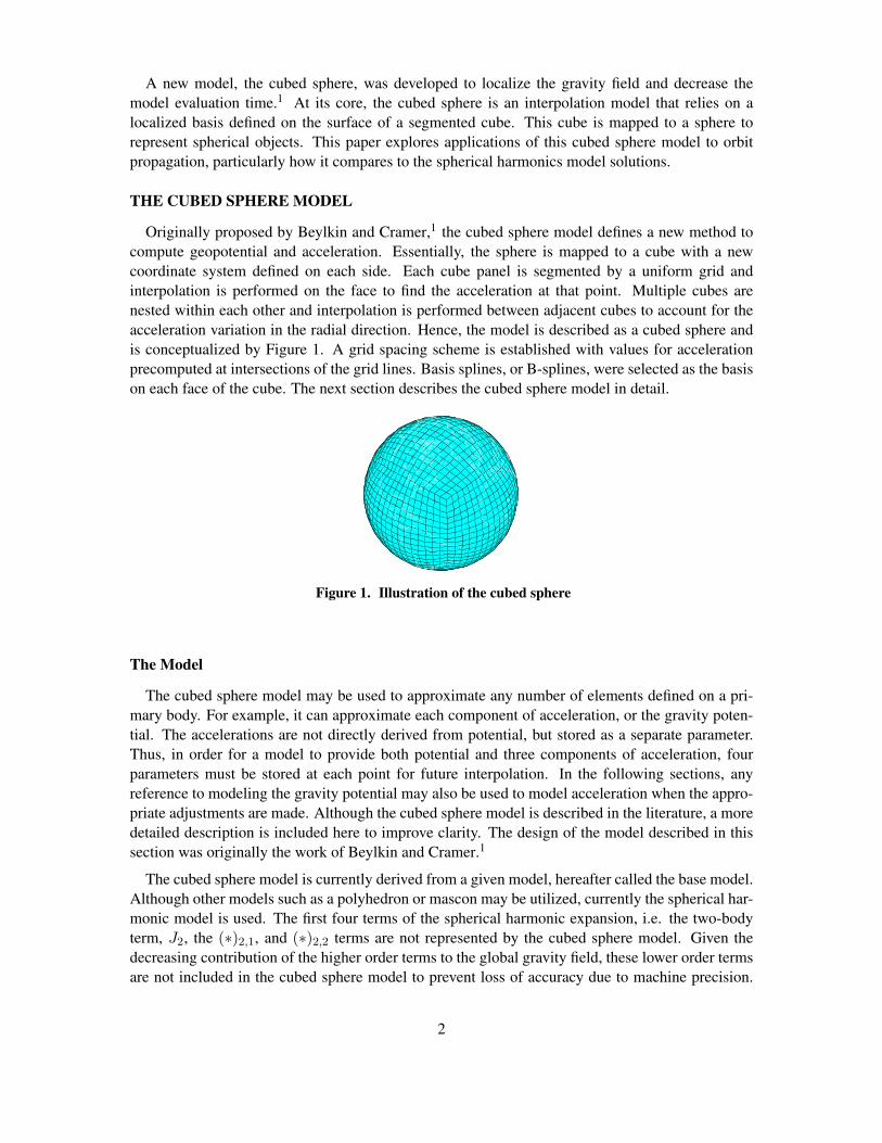
Originally proposed by Beylkin and Cramer,1 the cubed sphere model defines a new method tocompute geopotential and acceleration. Essentially, the sphere is mapped to a cube with a newcoordinate system defined on each side. Each cube panel is segmented by a uniform grid andinterpolation is performed on the face to find the acceleration at that point. Multiple cubes arenested within each other and interpolation is performed between adjacent cubes to account for theacceleration variation in the radial direction. Hence, the model is described as a cubed sphere andis conceptualized by Figure 1. A grid spacing scheme is established with values for accelerationprecomputed at intersections of the grid lines. Basis splines, or B-splines, were selected as the basison each face of the cube. The next section describes the cubed sphere model in detail.

Figure 1. Illustration of the cubed sphere

The Model

The cubed sphere model may be used to approximate any number of elements defined on a pri-mary body. For example, it can approximate each component of acceleration, or the gravity poten-tial. The accelerations are not directly derived from potential, but stored as a separate parameter.Thus, in order for a model to provide both potential and three components of acceleration, fourparameters must be stored at each point for future interpolation. In the following sections, anyreference to modeling the gravity potential may also be used to model acceleration when the appro-priate adjustments are made. Although the cubed sphere model is described in the literature, a moredetailed description is included here to improve clarity. The design of the model described in thissection was originally the work of Beylkin and Cramer.1

The cubed sphere model is currently derived from a given model, hereafter called the base model.Although other models such as a polyhedron or mascon may be utilized, currently the spherical har-monic model is used. The first four terms of the spherical harmonic expansion, i.e. the two-bodyterm, J2, the (∗)2,1, and (∗)2,2 terms are not represented by the cubed sphere model. Given thedecreasing contribution of the higher order terms to the global gravity field, these lower order termsare not included in the cubed sphere model to prevent loss of accuracy due to machine precision.

2

The geopotential values computed by the remaining base model are then used to define the ba-sis functions on the surface of the cube. Although other formulations are possible, B-splines arecurrently used. The method for deriving the cubed sphere will now be defined.

A major property of the cubed sphere model that must be defined is the grid size, N . Similar tothe degree and order of the spherical harmonic model, the grid size is a measure of model fidelityand defines the density of the grid on each cube panel. For a given altitude, the values of latitudeand longitude are segmented such that

θ = 2πx, φ = 2πy (2)

where x and y are discrete values in the range [0, 1) with spacing N−1. It may not be readilyapparent why the latitude, φ, is in the range [0, 2π), but this will be understood in a moment.

Latitude and longitude have been mapped to a two dimensional grid specified by x and y to solvefor the B-spline interpolation scheme. As described in the appendix, the interpolation coefficientsare easily derived in the Fourier domain for a periodic, two dimensional plane. If the grid variables xand y are 1-periodic, then the two-dimensional FFT algorithm may be used. The values of potentialat grid intersection points are used as data values. Hence, given a cube is comprised of six planes,the FFT algorithm provides a simplified method for representing the potential on the surface of acube.

If φ only varies from −π/2 to π/2, or 0 to π, then y is not 1-periodic. Thus, the formulation ofthe Earth’s geopotential must be duplicated to complete the period. The mathematical formulationof the new geopotential, Up, is then

Up(r, φ, θ) =

U(r, φ, θ) if 0 ≤ φ < φ,

U(r, 2π − φ, θ + π) if π ≤ φ < 2π(3)

and φ is now a value in the range [0, 2π) and 2π-periodic. Thus, y is now 1-periodic and theFFT algorithm is used to generate the B-spline interpolation coefficients. Note the doubling of thegeopotential model is only used to generate these coefficients.

To prevent grid distortion given the ambiguity of longitude at the poles, the Earth is rotated sothat the poles lie along the equator. This is equivalent to the transverse mercator map projection. Asecond x-y plane is generated after this rotation, with the FFT algorithm applied and a second set ofB-spline coefficients determined. This rotation is performed in the formulation of the base model.

B-spline coefficients have been defined over the flat surface of the two x-y grids. The gridsare then broken into appropriate segments to generate the faces of a cube. Each face, or panel,of the cube has a new x-y grid with axes defined over the range [−1, 1]. Four panels along themiddle latitudes are selected from the first plane, while the two remaining panels along the polesare selected from the second plane. Grid spacing is preserved along the face of the cube, howeverthe new panels are a quarter of the size. Thus, the size of the grid on each panel is N /4 by N /4.This property is used in the naming convention defined for a given model. A CS-X model is acubed sphere model where X corresponds to the grid size on a cube face , or N/4. Finally, thegeopotential model for the given shell has now been defined and is represented as a cube.

Additionally, a user specified number of nested, concentric shells is defined for interpolation inthe radial direction. Shell spacing is determined by defining a set number of points (hj) equally

3

spaced in the interval [0, 1]. Shell locations are then

R

rj= 1− h2

j (4)

where rj is the radial distance of the shell. These ratios, which represent a distance above theplanet’s surface in the range (0, 1], define shell locations. As the ratio approaches zero, the orbitradius approaches infinity. Shell density increases as altitude decreases, corresponding to the inversesquare relationship between geopotential and radius. The final shell at a radius of infinity is notcomputed. The model assumes eventual decay to zero of the spherical harmonic terms, thus thetwo-body equation will govern satellite dynamics.

These primary shells are modeled with each consisting of subshells for polynomial interpolationof a prescribed degree in the radial direction. For a fifth degree interpolation scheme, six subshellsare required. The spacing between subshells is mapped to the range [−1, 1] where zero correspondsto the midpoint between primary shells. The subshells are then located at the Chebyshev nodesbased on the degree of the polynomial. Chebyshev nodes were selected to minimize interpolationerror due to node selection. Each primary and subshell is independent of all others, thus there isno coupling in model generation. B-spline coefficients for each shell are generated as previouslydescribed using the applicable altitude for the evaluation of Eq. 3. A total of (l + 1) ×M shellsare computed where l is the degree of the interpolating polynomial and M is the number of primaryshells. It is important to note the mapping to the cube is simply used for data storage and solvingfor the spline coefficients. All parameters described by the model, more specifically components ofacceleration, are still represented in the spherical coordinate system. The cube provides a uniformgrid for B-spline coefficient determination and a data structure for faster computation.

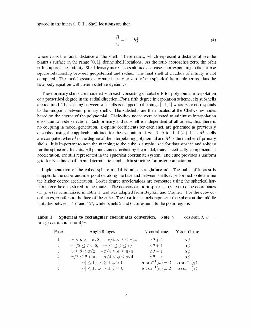
Implementation of the cubed sphere model is rather straightforward. The point of interest ismapped to the cube, and interpolation along the face and between shells is performed to determinethe higher degree acceleration. Lower degree accelerations are computed using the spherical har-monic coefficients stored in the model. The conversion from spherical (φ, λ) to cube coordinates(x, y, n) is summarized in Table 1, and was adapted from Beylkin and Cramer.1 For the cube co-ordinates, n refers to the face of the cube. The first four panels represent the sphere at the middlelatitudes between -45 and 45, while panels 5 and 6 correspond to the polar regions.

Table 1 Spherical to rectangular coordinates conversion. Note γ = cosφ sin θ, ω =tanφ/ cos θ, and α = 4/π.

Face Angle Ranges X-coordinate Y-coordinate

1 −π ≤ θ < −π/2, −π/4 ≤ φ ≤ π/4 αθ + 3 αφ2 −π/2 ≤ θ < 0, −π/4 ≤ φ ≤ π/4 αθ + 1 αφ3 0 ≤ θ < π/2, −π/4 ≤ φ ≤ π/4 αθ − 1 αφ4 π/2 ≤ θ < π, −π/4 ≤ φ ≤ π/4 αθ − 3 αφ

5 |γ| ≤ 1, |ω| ≥ 1, φ > 0 α tan−1(ω)± 2 α sin−1(γ)6 |γ| ≤ 1, |ω| ≥ 1, φ < 0 α tan−1(ω)± 2 α sin−1(γ)

4

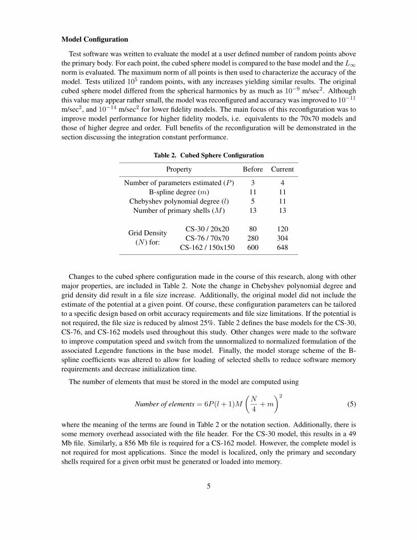
Model Configuration

Test software was written to evaluate the model at a user defined number of random points abovethe primary body. For each point, the cubed sphere model is compared to the base model and theL∞norm is evaluated. The maximum norm of all points is then used to characterize the accuracy of themodel. Tests utilized 105 random points, with any increases yielding similar results. The originalcubed sphere model differed from the spherical harmonics by as much as 10−9 m/sec2. Althoughthis value may appear rather small, the model was reconfigured and accuracy was improved to 10−11

m/sec2, and 10−14 m/sec2 for lower fidelity models. The main focus of this reconfiguration was toimprove model performance for higher fidelity models, i.e. equivalents to the 70x70 models andthose of higher degree and order. Full benefits of the reconfiguration will be demonstrated in thesection discussing the integration constant performance.

Table 2. Cubed Sphere Configuration

Property Before Current

Number of parameters estimated (P ) 3 4B-spline degree (m) 11 11

Chebyshev polynomial degree (l) 5 11Number of primary shells (M ) 13 13

Grid Density(N ) for:

CS-30 / 20x20 80 120CS-76 / 70x70 280 304

CS-162 / 150x150 600 648

Changes to the cubed sphere configuration made in the course of this research, along with othermajor properties, are included in Table 2. Note the change in Chebyshev polynomial degree andgrid density did result in a file size increase. Additionally, the original model did not include theestimate of the potential at a given point. Of course, these configuration parameters can be tailoredto a specific design based on orbit accuracy requirements and file size limitations. If the potential isnot required, the file size is reduced by almost 25%. Table 2 defines the base models for the CS-30,CS-76, and CS-162 models used throughout this study. Other changes were made to the softwareto improve computation speed and switch from the unnormalized to normalized formulation of theassociated Legendre functions in the base model. Finally, the model storage scheme of the B-spline coefficients was altered to allow for loading of selected shells to reduce software memoryrequirements and decrease initialization time.

The number of elements that must be stored in the model are computed using

Number of elements = 6P (l + 1)M(N

4+m

)2

(5)

where the meaning of the terms are found in Table 2 or the notation section. Additionally, there issome memory overhead associated with the file header. For the CS-30 model, this results in a 49Mb file. Similarly, a 856 Mb file is required for a CS-162 model. However, the complete model isnot required for most applications. Since the model is localized, only the primary and secondaryshells required for a given orbit must be generated or loaded into memory.

5

Experimental results demonstrate the evaluation time of the cubed sphere model is slightly morethan the 20x20 spherical harmonics. As the model grid density is increased, corresponding to anincrease in model fidelity, evaluation time does not increase. The B-spline coefficients are organizedsuch that no search is necessary. If the degree of the interpolating functions remains constant foreach grid size, model evaluation time remains constant. Thus, speed-up factors compared to thespherical harmonics increases with model fidelity.

COMPARISONS TO THE SPHERICAL HARMONICS MODEL

After the cubed sphere was fully developed, it was compared to the spherical harmonics model.The GGM02C10 model was selected as both the base model of the cubed sphere and the basis ofcomparison for the following tests. Evaluations included a comparison of the integration constant,spatial comparisons of the models in the form of gravity anomaly plots, and finally the propagatedorbits themselves.

The TurboProp orbit integration package11 was used to minimize software development time.This software provides integration tools implemented in C that are compatible with MATLAB.Unreleased versions are also compatible with Python. The cubed sphere model, along with the nec-essary interface code, was implemented within the TurboProp framework. However, the softwarecan be easily ported to other packages. For the following tests requiring orbit propagation, the Tur-boProp Runge Kutta 7(8) integrator was used to simplify integrator setup with automated executionfor a variety of initial conditions. Other integrators were tested, including symplectic Runge Kuttaalgorithms, but yielded similar results. The absolute integration tolerance was set to 10−12.

Orbits were propagated for 24 hours with a variety of initial conditions and states output every20 seconds. The initial orbit altitude was varied between 100 and 1,000 km at 50 km intervals.Model accuracy relative to the spherical harmonics decreases with reductions in altitude, howevermost satellites orbit at or above 300 km. Thus, altitude specific results in the following sections areprovided at 300 km. The right ascension of the ascending node (Ω) ranged from 0 to 180 in 5

increments, while the inclination varied from and 0 to 85 in 2.5 intervals. All other orbit elementswere initially set to zero. The inclination was intentionally kept below 85 to avoid the singularityat the poles in the classical formulation of the spherical harmonics. Thus, for each altitude, 1,295orbits were tested. The Greenwich sidereal time was set to 0 at the epoch time, with an Earthrotation rate of 360 per solar day. The planetary radius and gravitation parameter were set to theappropriate value as determined by the base model. Each set of initial conditions was propagatedusing the cubed sphere and the corresponding base model. The trajectories were differenced and3D RMS differences were calculated and stored. Any reference to an orbit propagation “error” isdefined as the difference between the cubed sphere and the spherical harmonic model orbits. Thethree models described in Table 2 were tested.

Integration (Jacobi) Constant Comparisons

A given geopotential model must satisfy the Laplace equation,

∇2U =∂2U

∂x2+∂2U

∂y2+∂2U

∂z2= 0 (6)

Unfortunately, there is no direct method to calculate the second derivatives of the cubed sphere.Parameters could be added to the model to estimate these values, similar to the those modeling

6

the geopotential and the gravity accelerations. However, this will drastically increase file size.Additionally, finite differencing would only be an approximation.

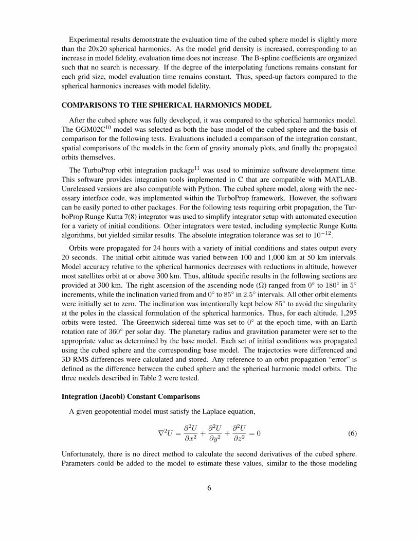
Instead of testing the cubed sphere under the Laplace criterion, another technique using theJacobi-like integration constant,12

K =~r · ~r

2−[µr− U(~r, t)

]− ~ω · (~r × ~r) (7)

is used. This constant assumes the geopotential is a time varying potential, which is valid due toEarth rotation. Here, ~ω is the angular velocity of the primary body. For a valid gravity model anda propagated orbit, K must remain constant over time, or K − K equals zero. In practice, theconstant fluctuates due to the numerical integration process and errors in the estimate of the gravityfield.

0 5 10 15 20 25−20

−10

0

10

20

Ch

ang

e (m

m2 /s

2 )

Integration Constant Change for Old Cubed Sphere Model

Sph. Harm.

Cub. Sph.

0 5 10 15 20 25−1

−0.5

0

0.5

Hours Since Epoch

Ch

ang

e (m

m2 /s

2 )

Integration Constant Change for New Cubed Sphere Model

Figure 2 Changes in integration constant with the new CS-162 model configurationfor an orbit with an inclination of 15 and right ascension of 50 at a 300 km altitude.

As mentioned previously, the cubed sphere was reconfigured to improve accuracy. The prin-ciple motivation for this alteration was improving the integration constant performance. Figure 2illustrates the extent of the improvement. Previously, the cubed sphere integration constant wasconsistently 1-3 orders of magnitude greater. This result would reduce the validity of the model forapplications requiring long term orbit propagation, thus the model was reconfigured. In some cases,such as this example, the integration constant performs better than the spherical harmonics with thenew configuration.

Table 3. Fraction of runs where O(K-K) is less than the other model.

Model Cubed Sphere Spherical Harmonics

CS-30 0.024% 0.020%CS-76 0.012% 0.008%CS-162 0.264% 0.272%

A major concern when comparing the variations in the integration constant for the cubed sphereand the spherical harmonics models is the relative magnitude of the fluctuations. In some cases, the

7

magnitude of the variations of the cubed sphere were as much as an order of magnitude less thanthe spherical harmonics, and vice versa. Table 3 provides the percentage of the 24,605 runs for eachmodel that exhibited this behavior. In most cases, the order of magnitude of the fluctuations wasthe same. However, a small percentage of the tests yielded integration constant changes an order ofmagnitude less for one model when compared to the other. In the case of the CS-162 model, wherethe percentage of runs sharply increased, tests at altitudes at or below 250 km exhibited the largerfluctuations.

−0.6

−0.4

−0.2

0.0

0.2

0.4

0.6

0.8Max(mm^2/s^2)

Max K-Kand Trend Differences

200 400 600 800 1000

Orbit Altitude (km)

−0.04

−0.03

−0.02

−0.01

0.00

0.01

0.02

0.03

0.04

Trend(mm^2/s^2/hr.)

Mean

Median

Min

Max

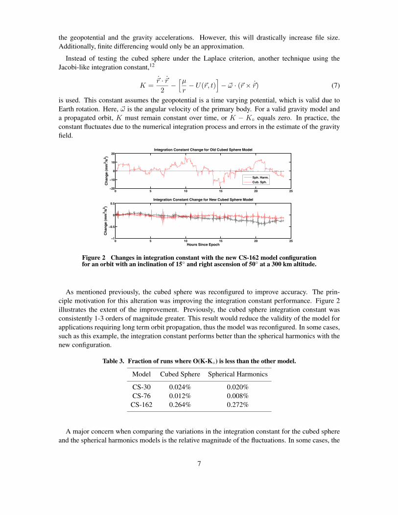
Figure 3 Comparison of the integration constant variations for the CS-30 model withthe spherical harmonics base model. Error bars are 1-σ.

In addition to the magnitude of the variations, any trends in the integration constant variationsshould be considered. For a given orbit, the maximum of the absolute values of the fluctuations forthe cubed sphere and the spherical harmonics were differenced. Similarly, a linear fit was performedon the integration constant change for a single orbit and the differences in the absolute values of theslopes for the models were calculated. Statistics were assembled on the model performance foreach altitude, with the results provided in Figure 3 for the CS-30 model. In both cases, a negativenumber means the cubed sphere model exhibited smaller variations or trends in the integrationconstant. For the slope in the trend line, units are designated as mm2/sec2/hour. Since the units ofthe integration constant are mm2/sec2, the mixture of seconds and hours is intended to preserve thechange of the integration constant over a given time period. For altitudes below 400 km, the meanand median magnitude differences indicate the spherical harmonics model slightly outperforms thecubed sphere. However, the average difference drops to nearly zero above 400 km. The maximumand minimum differences remain consistent. Given the mean and median differences in the trendline slope are around zero with 1-σ values within 0.01 mm2/sec2/hour, the two models typicallyhave the same long term trend.

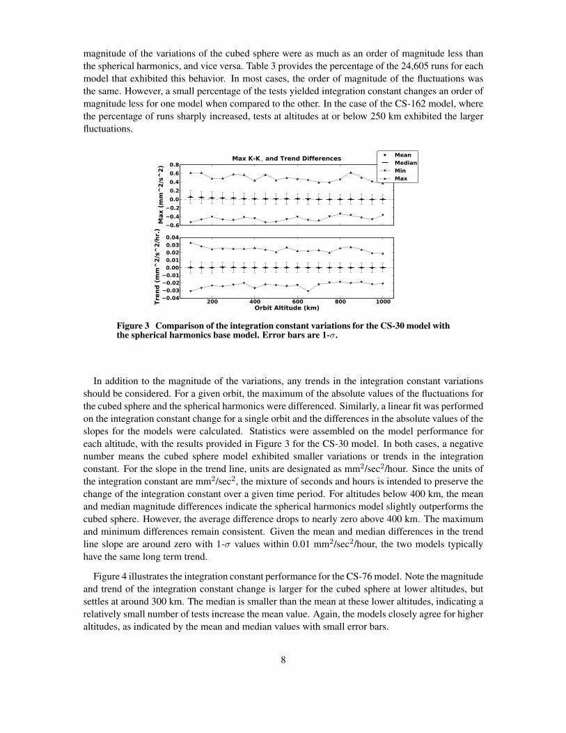
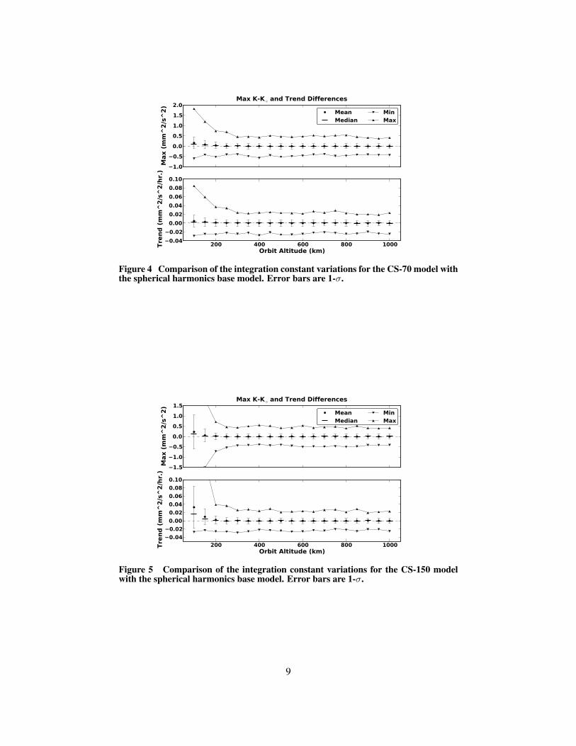
Figure 4 illustrates the integration constant performance for the CS-76 model. Note the magnitudeand trend of the integration constant change is larger for the cubed sphere at lower altitudes, butsettles at around 300 km. The median is smaller than the mean at these lower altitudes, indicating arelatively small number of tests increase the mean value. Again, the models closely agree for higheraltitudes, as indicated by the mean and median values with small error bars.

8

−1.0

−0.5

0.0

0.5

1.0

1.5

2.0

Max(mm^2/s^2)

Max K-Kand Trend Differences

Mean

Median

Min

Max

200 400 600 800 1000

Orbit Altitude (km)

−0.04

−0.02

0.00

0.02

0.04

0.06

0.08

0.10

Trend(mm^2/s^2/hr.)

Figure 4 Comparison of the integration constant variations for the CS-70 model withthe spherical harmonics base model. Error bars are 1-σ.

−1.5

−1.0

−0.5

0.0

0.5

1.0

1.5

Max(mm^2/s^2)

Max K-Kand Trend Differences

Mean

Median

Min

Max

200 400 600 800 1000

Orbit Altitude (km)

−0.04

−0.02

0.00

0.02

0.04

0.06

0.08

0.10

Trend(mm^2/s^2/hr.)

Figure 5 Comparison of the integration constant variations for the CS-150 modelwith the spherical harmonics base model. Error bars are 1-σ.

9

Results for the CS-162 model are provided in Figure 5. Note some extreme values have beentruncated to improve visibility of performance statistics at higher altitudes. In the case of the dif-ferences in the magnitude differences, the minimum values for the 100 and 150 km orbits are -3.39and -1.51 mm2/sec2, respectively. The maximum values are 5.20 and 1.79 mm2/sec2. In the caseof the trend slope differences, the missing maximums are 0.44 and 0.14 mm2/sec2/hour. Like theCS-76 model, differences between the cubed sphere and spherical harmonics models are greater atlower altitudes. This trend remains consistent through the remaining tests, and is attributed to thegreater differences in the gravity anomalies at lower altitudes seen in the next section. In this case,the differences in the models settles around 250 km.

Gravity Anomaly Comparisons

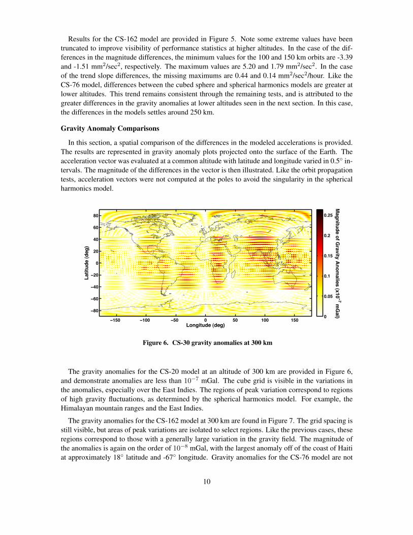
In this section, a spatial comparison of the differences in the modeled accelerations is provided.The results are represented in gravity anomaly plots projected onto the surface of the Earth. Theacceleration vector was evaluated at a common altitude with latitude and longitude varied in 0.5 in-tervals. The magnitude of the differences in the vector is then illustrated. Like the orbit propagationtests, acceleration vectors were not computed at the poles to avoid the singularity in the sphericalharmonics model.

Longitude (deg)

Lat

itu

de

(deg

)

−150 −100 −50 0 50 100 150

−80

−60

−40

−20

0

20

40

60

80

Mag

nitu

de o

f Gravity A

no

malies (x10

−7 mG

al)0

0.05

0.1

0.15

0.2

0.25

Figure 6. CS-30 gravity anomalies at 300 km

The gravity anomalies for the CS-20 model at an altitude of 300 km are provided in Figure 6,and demonstrate anomalies are less than 10−7 mGal. The cube grid is visible in the variations inthe anomalies, especially over the East Indies. The regions of peak variation correspond to regionsof high gravity fluctuations, as determined by the spherical harmonics model. For example, theHimalayan mountain ranges and the East Indies.

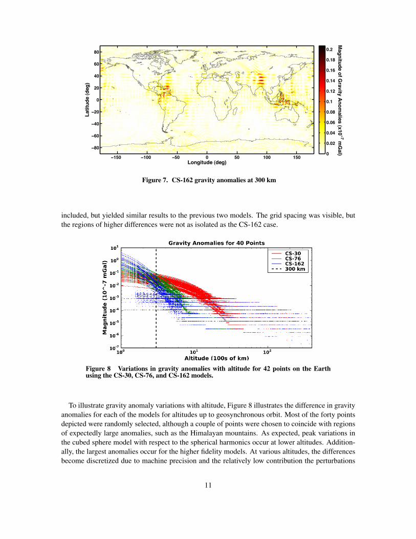
The gravity anomalies for the CS-162 model at 300 km are found in Figure 7. The grid spacing isstill visible, but areas of peak variations are isolated to select regions. Like the previous cases, theseregions correspond to those with a generally large variation in the gravity field. The magnitude ofthe anomalies is again on the order of 10−8 mGal, with the largest anomaly off of the coast of Haitiat approximately 18 latitude and -67 longitude. Gravity anomalies for the CS-76 model are not

10

Longitude (deg)

Lat

itu

de

(deg

)

−150 −100 −50 0 50 100 150

−80

−60

−40

−20

0

20

40

60

80

Mag

nitu

de o

f Gravity A

no

malies (x10

−7 mG

al)0

0.02

0.04

0.06

0.08

0.1

0.12

0.14

0.16

0.18

0.2

Figure 7. CS-162 gravity anomalies at 300 km

included, but yielded similar results to the previous two models. The grid spacing was visible, butthe regions of higher differences were not as isolated as the CS-162 case.

Figure 8 Variations in gravity anomalies with altitude for 42 points on the Earthusing the CS-30, CS-76, and CS-162 models.

To illustrate gravity anomaly variations with altitude, Figure 8 illustrates the difference in gravityanomalies for each of the models for altitudes up to geosynchronous orbit. Most of the forty pointsdepicted were randomly selected, although a couple of points were chosen to coincide with regionsof expectedly large anomalies, such as the Himalayan mountains. As expected, peak variations inthe cubed sphere model with respect to the spherical harmonics occur at lower altitudes. Addition-ally, the largest anomalies occur for the higher fidelity models. At various altitudes, the differencesbecome discretized due to machine precision and the relatively low contribution the perturbations

11

modeled by the cubed sphere have on the overall gravity acceleration.

For the CS-162 model, there is a region below 300 km and around 10−10 mGal where the varia-tions are periodic. In this case, the difference is close to the machine precision and is not determinedby the grid spacing. Given the Chebyshev interpolation between shells, approximation error willvary based on proximity to the nearby shells. Thus, as the altitude increases for this point in Figure8, the error periodically increases and decreases.

Orbit Propagation Comparisons

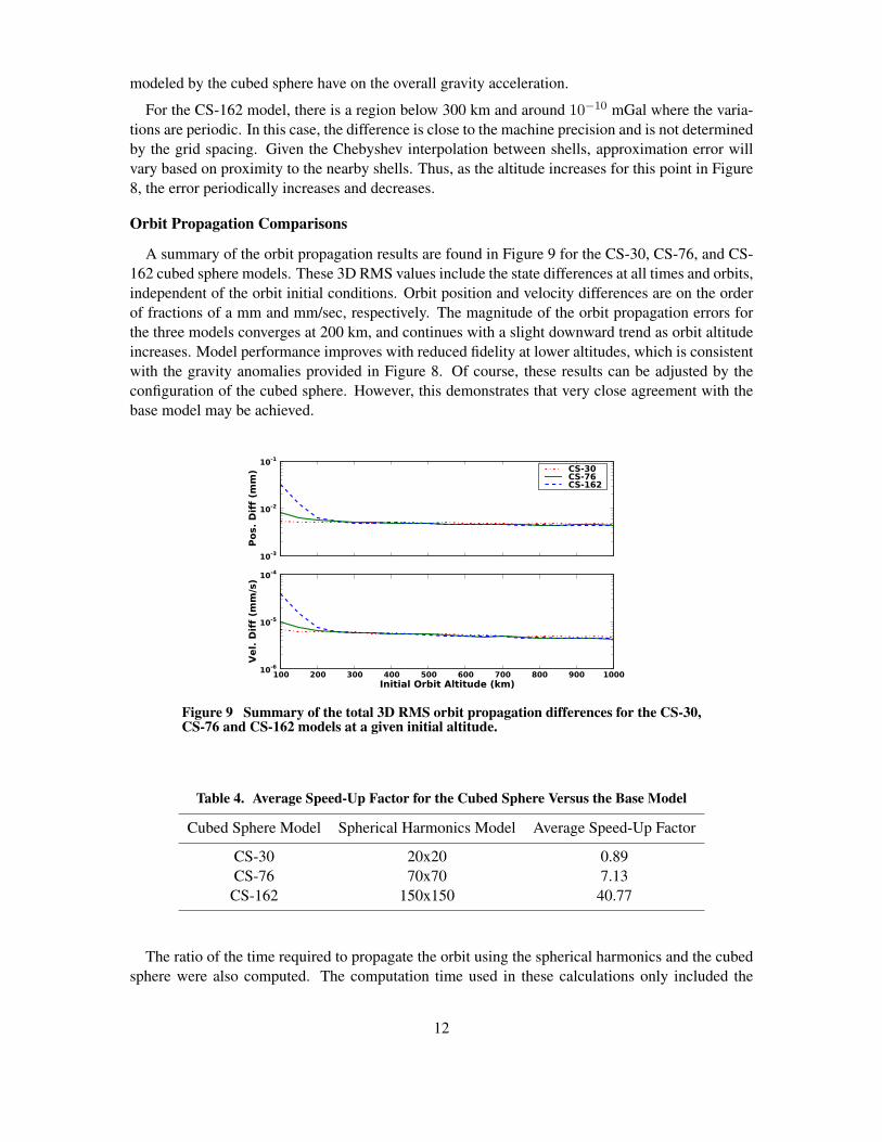
A summary of the orbit propagation results are found in Figure 9 for the CS-30, CS-76, and CS-162 cubed sphere models. These 3D RMS values include the state differences at all times and orbits,independent of the orbit initial conditions. Orbit position and velocity differences are on the orderof fractions of a mm and mm/sec, respectively. The magnitude of the orbit propagation errors forthe three models converges at 200 km, and continues with a slight downward trend as orbit altitudeincreases. Model performance improves with reduced fidelity at lower altitudes, which is consistentwith the gravity anomalies provided in Figure 8. Of course, these results can be adjusted by theconfiguration of the cubed sphere. However, this demonstrates that very close agreement with thebase model may be achieved.

10-3

10-2

10-1

Pos.Diff(mm) CS-30

CS-76CS-162

100 200 300 400 500 600 700 800 900 1000

Initial Orbit Altitude (km)

10-6

10-5

10-4

Vel.Diff(mm/s)

Figure 9 Summary of the total 3D RMS orbit propagation differences for the CS-30,CS-76 and CS-162 models at a given initial altitude.

Table 4. Average Speed-Up Factor for the Cubed Sphere Versus the Base Model

Cubed Sphere Model Spherical Harmonics Model Average Speed-Up Factor

CS-30 20x20 0.89CS-76 70x70 7.13CS-162 150x150 40.77

The ratio of the time required to propagate the orbit using the spherical harmonics and the cubedsphere were also computed. The computation time used in these calculations only included the

12

execution of the RK78 algorithm, and did not include file load times or software initialization. Asexpected, the file load time for the cubed sphere is longer than the spherical harmonics, howeverthis can be mitigated through implementation. The speed-up factors are given in Table 4. Afterthe model reconfiguration, specifically the increase in the degree of the polynomial interpolationbetween shells, the evaluation time of the model increased. Hence, the spherical harmonics isslightly faster for models of degree 20 and lower. Thus, research into altering the configuration ofthe lower fidelity models, specifically reducing the polynomial degree to reduce computation time,is planned.

0 10 20 30 40 50 60 70 80

Inclination (deg)

0

20

40

60

80

100

120

140

160

180

RightAscension(deg)

0.00

0.25

0.50

0.75

1.00

1.25

1.50

1.75

2.00

3DRMSPositio

nError(10^-2

mm)

0.0 0.2 0.4 0.6 0.8 1.0 1.2 1.4 1.6 1.8

3D RMS Position Error (10^-2 mm)

0

20

40

60

80

100

120

NumberofRuns

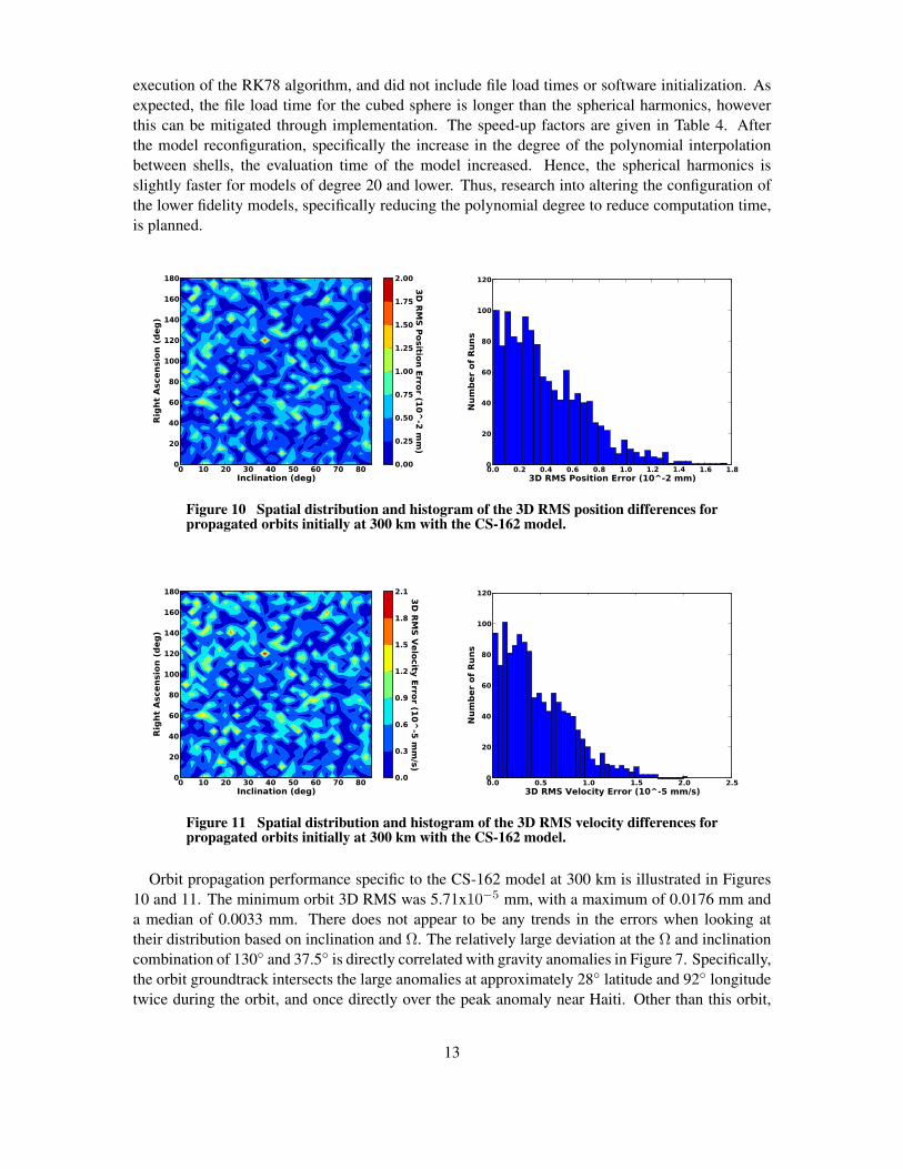
Figure 10 Spatial distribution and histogram of the 3D RMS position differences forpropagated orbits initially at 300 km with the CS-162 model.

0 10 20 30 40 50 60 70 80

Inclination (deg)

0

20

40

60

80

100

120

140

160

180

RightAscension(deg)

0.0

0.3

0.6

0.9

1.2

1.5

1.8

2.1

3DRMSVelocity

Error(10^-5

mm/s)

0.0 0.5 1.0 1.5 2.0 2.5

3D RMS Velocity Error (10^-5 mm/s)

0

20

40

60

80

100

120

NumberofRuns

Figure 11 Spatial distribution and histogram of the 3D RMS velocity differences forpropagated orbits initially at 300 km with the CS-162 model.

Orbit propagation performance specific to the CS-162 model at 300 km is illustrated in Figures10 and 11. The minimum orbit 3D RMS was 5.71x10−5 mm, with a maximum of 0.0176 mm anda median of 0.0033 mm. There does not appear to be any trends in the errors when looking attheir distribution based on inclination and Ω. The relatively large deviation at the Ω and inclinationcombination of 130 and 37.5 is directly correlated with gravity anomalies in Figure 7. Specifically,the orbit groundtrack intersects the large anomalies at approximately 28 latitude and 92 longitudetwice during the orbit, and once directly over the peak anomaly near Haiti. Other than this orbit,

13

all others are within 0.015 mm of the spherical harmonics. The spatial distribution of the velocityerrors roughly corresponds to the position errors, with a minimum of 2.503x10−8 mm/sec and amaximum of 2.037x10−5 mm/sec. The median 3D RMS velocity error was 3.80x10−6 mm/sec.

0.0 0.5 1.0 1.5 2.0

3D RMS Position Error (10^-2 mm)

0

20

40

60

80

100

120

NumberofRuns

0.0 0.5 1.0 1.5 2.0 2.5

3D RMS Velocity Error (10^-5 mm/s)

0

20

40

60

80

100

120

NumberofRuns

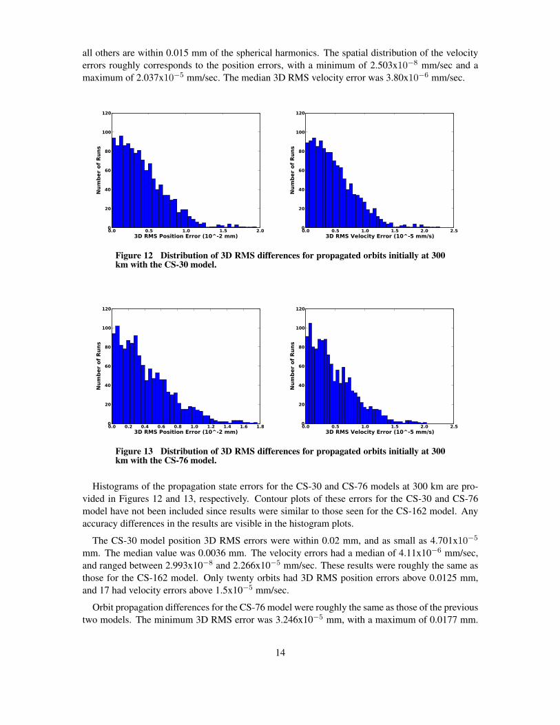
Figure 12 Distribution of 3D RMS differences for propagated orbits initially at 300km with the CS-30 model.

0.0 0.2 0.4 0.6 0.8 1.0 1.2 1.4 1.6 1.8

3D RMS Position Error (10^-2 mm)

0

20

40

60

80

100

120

NumberofRuns

0.0 0.5 1.0 1.5 2.0 2.5

3D RMS Velocity Error (10^-5 mm/s)

0

20

40

60

80

100

120

NumberofRuns

Figure 13 Distribution of 3D RMS differences for propagated orbits initially at 300km with the CS-76 model.

Histograms of the propagation state errors for the CS-30 and CS-76 models at 300 km are pro-vided in Figures 12 and 13, respectively. Contour plots of these errors for the CS-30 and CS-76model have not been included since results were similar to those seen for the CS-162 model. Anyaccuracy differences in the results are visible in the histogram plots.

The CS-30 model position 3D RMS errors were within 0.02 mm, and as small as 4.701x10−5

mm. The median value was 0.0036 mm. The velocity errors had a median of 4.11x10−6 mm/sec,and ranged between 2.993x10−8 and 2.266x10−5 mm/sec. These results were roughly the same asthose for the CS-162 model. Only twenty orbits had 3D RMS position errors above 0.0125 mm,and 17 had velocity errors above 1.5x10−5 mm/sec.

Orbit propagation differences for the CS-76 model were roughly the same as those of the previoustwo models. The minimum 3D RMS error was 3.246x10−5 mm, with a maximum of 0.0177 mm.

14

The median was 0.0033 mm. The velocity errors were less than 2.042x10−5 mm/sec, with a medianof 3.788x10−6 mm/sec. The minimum error was 2.042x10−8 mm/sec.

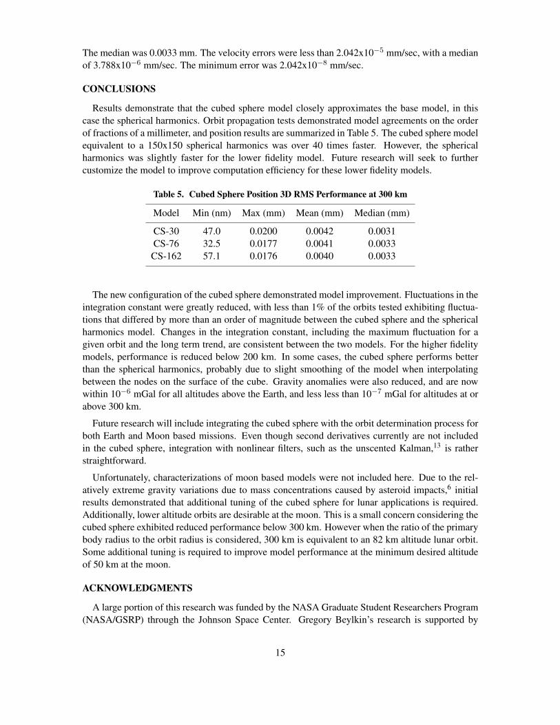
CONCLUSIONS

Results demonstrate that the cubed sphere model closely approximates the base model, in thiscase the spherical harmonics. Orbit propagation tests demonstrated model agreements on the orderof fractions of a millimeter, and position results are summarized in Table 5. The cubed sphere modelequivalent to a 150x150 spherical harmonics was over 40 times faster. However, the sphericalharmonics was slightly faster for the lower fidelity model. Future research will seek to furthercustomize the model to improve computation efficiency for these lower fidelity models.

Table 5. Cubed Sphere Position 3D RMS Performance at 300 km

Model Min (nm) Max (mm) Mean (mm) Median (mm)

CS-30 47.0 0.0200 0.0042 0.0031CS-76 32.5 0.0177 0.0041 0.0033CS-162 57.1 0.0176 0.0040 0.0033

The new configuration of the cubed sphere demonstrated model improvement. Fluctuations in theintegration constant were greatly reduced, with less than 1% of the orbits tested exhibiting fluctua-tions that differed by more than an order of magnitude between the cubed sphere and the sphericalharmonics model. Changes in the integration constant, including the maximum fluctuation for agiven orbit and the long term trend, are consistent between the two models. For the higher fidelitymodels, performance is reduced below 200 km. In some cases, the cubed sphere performs betterthan the spherical harmonics, probably due to slight smoothing of the model when interpolatingbetween the nodes on the surface of the cube. Gravity anomalies were also reduced, and are nowwithin 10−6 mGal for all altitudes above the Earth, and less less than 10−7 mGal for altitudes at orabove 300 km.

Future research will include integrating the cubed sphere with the orbit determination process forboth Earth and Moon based missions. Even though second derivatives currently are not includedin the cubed sphere, integration with nonlinear filters, such as the unscented Kalman,13 is ratherstraightforward.

Unfortunately, characterizations of moon based models were not included here. Due to the rel-atively extreme gravity variations due to mass concentrations caused by asteroid impacts,6 initialresults demonstrated that additional tuning of the cubed sphere for lunar applications is required.Additionally, lower altitude orbits are desirable at the moon. This is a small concern considering thecubed sphere exhibited reduced performance below 300 km. However when the ratio of the primarybody radius to the orbit radius is considered, 300 km is equivalent to an 82 km altitude lunar orbit.Some additional tuning is required to improve model performance at the minimum desired altitudeof 50 km at the moon.

ACKNOWLEDGMENTS

A large portion of this research was funded by the NASA Graduate Student Researchers Program(NASA/GSRP) through the Johnson Space Center. Gregory Beylkin’s research is supported by

15

AFOSR grant FA9550-07-1-0135. The authors would like to thank Keric Hill, formerly of theColorado Center for Astrodynamics Research, who wrote the early versions of TurboProp.

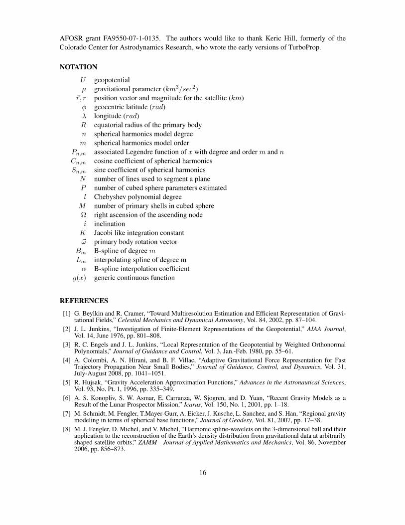
NOTATION

U geopotentialµ gravitational parameter (km3/sec2)

~r, r position vector and magnitude for the satellite (km)φ geocentric latitude (rad)λ longitude (rad)R equatorial radius of the primary bodyn spherical harmonics model degreem spherical harmonics model order

Pn,m associated Legendre function of x with degree and order m and nCn,m cosine coefficient of spherical harmonicsSn,m sine coefficient of spherical harmonicsN number of lines used to segment a planeP number of cubed sphere parameters estimatedl Chebyshev polynomial degree

M number of primary shells in cubed sphereΩ right ascension of the ascending nodei inclinationK Jacobi like integration constant~ω primary body rotation vector

Bm B-spline of degree mLm interpolating spline of degree mα B-spline interpolation coefficient

g(x) generic continuous function

REFERENCES

[1] G. Beylkin and R. Cramer, “Toward Multiresolution Estimation and Efficient Representation of Gravi-tational Fields,” Celestial Mechanics and Dynamical Astronomy, Vol. 84, 2002, pp. 87–104.

[2] J. L. Junkins, “Investigation of Finite-Element Representations of the Geopotential,” AIAA Journal,Vol. 14, June 1976, pp. 801–808.

[3] R. C. Engels and J. L. Junkins, “Local Representation of the Geopotential by Weighted OrthonormalPolynomials,” Journal of Guidance and Control, Vol. 3, Jan.-Feb. 1980, pp. 55–61.

[4] A. Colombi, A. N. Hirani, and B. F. Villac, “Adaptive Gravitational Force Representation for FastTrajectory Propagation Near Small Bodies,” Journal of Guidance, Control, and Dynamics, Vol. 31,July-August 2008, pp. 1041–1051.

[5] R. Hujsak, “Gravity Acceleration Approximation Functions,” Advances in the Astronautical Sciences,Vol. 93, No. Pt. 1, 1996, pp. 335–349.

[6] A. S. Konopliv, S. W. Asmar, E. Carranza, W. Sjogren, and D. Yuan, “Recent Gravity Models as aResult of the Lunar Prospector Mission,” Icarus, Vol. 150, No. 1, 2001, pp. 1–18.

[7] M. Schmidt, M. Fengler, T.Mayer-Gurr, A. Eicker, J. Kusche, L. Sanchez, and S. Han, “Regional gravitymodeling in terms of spherical base functions,” Journal of Geodesy, Vol. 81, 2007, pp. 17–38.

[8] M. J. Fengler, D. Michel, and V. Michel, “Harmonic spline-wavelets on the 3-dimensional ball and theirapplication to the reconstruction of the Earth’s density distribution from gravitational data at arbitrarilyshaped satellite orbits,” ZAMM - Journal of Applied Mathematics and Mechanics, Vol. 86, November2006, pp. 856–873.

16

[9] R. Mautz, B. Schaffrin, C. K. Shum, and S.-C. Han, Earth observation with CHAMP, results from threeyears in orbit, ch. Regional Geoid Undulations from CHAMP, Represented by Locally Supported BasisFunctions, pp. 230–236. Berlin Heidelberg New York: Springer, 2004.

[10] B. Tapley, J. Ries, S. Bettadpur, D. Chambers, M. Cheng, F. Condi, B. Gunter, Z. Kang, P. Nagel,R. Pastor, T. Pekker, S. Poole, and F. Wang, “GGM02 - An Improved Earth Gravity Field Model fromGRACE,” Journal of Geodesy, DOI 10.1007/s00190-005-0480-z, 2005.

[11] K. Hill and B. A. Jones, TurboProp Version 3.3. Colorado Center for Astrodynamics Research,http://ccar.colorado.edu/geryon/software.html, September 2008.

[12] V. R. Bond and M. C. Allman, Modern Astrodynamics. Princeton, New Jersey: Princeton UniversityPress, 1996.

[13] S. J. Julier and J. K. Uhlmann, “A New Extension of the Kalman Filter to Nonlinear Systems,” Proceed-ings of SPIE, Vol. 3068, 1997, pp. 182–193.

[14] C. K. Chui, An Introduction to Wavelets, Vol. One of Wavelet Analysis and Its Applications. Boston:Academic Press, Inc., first ed., 1992.

APPENDIX: BASIS SPLINES

A simple way to introduce basis splines (or B-splines) is to define them as

Bm(x) = (Bm−1 ∗B0)(x), (8)

where

B0(x) =

1, |x| ≤ 1

2

0, otherwise.(9)

Thus, Bm is a piecewise polynomial of degree m. On taking the Fourier transform of B0,∫ +∞

−∞B0(x)e−2πixξdx =

sinπξπξ

, (10)

we obtain ∫ +∞

∞Bm(x)e−2πixξdx =

(sinπξπξ

)m+1

. (11)

We only consider B-splines of odd degree and note that in such case the mth degree B-spline isnonzero only in the interval [−(m + 1)/2, (m + 1)/2]. For our purposes, we use a periodizedversion of B-splines on the interval [0, 1]. Subdividing [0, 1] into N = 2k subintervals, whereN ≥ m+ 1 (in practice N m+ 1), we consider the basis of B-splines on this subdivision,

Bm(Nx− j)j=0,1,...,2k−1 .

Let us consider a function g(x) that may be written as

g(x) =N−1∑j=0

αjBm(Nx− j). (12)

Instead of using the basis of B-splines, we may also write the same function as

g(x) =N−1∑j=0

γjLm(Nx− j) (13)

17

where Lm are interpolating splines, i.e.

Lm(l) = δl,0, (14)

where l is an integer. The definition of interpolating splines implies that the coefficients in Eq. 13are, in fact, the values of the function g(x) on the lattice,

g(l/N) = γl. (15)

In our problem, we are given the values γl = g(l/N) and need to find the coefficients αj in Eq.12. We have ∫ 1

0Bm(Nx− j)e−2πixndx =

1NBm

( nN

)e−2πijn/N , (16)

and computing the Fourier coefficients of g in Eq. 12, we obtain

gn =

1N

N−1∑j=0

αje−2πijn/N

Bm

( nN

)= αnBm

( nN

). (17)

Similarly, we compute the Fourier coefficients of g in terms of interpolating splines,

gn =

1N

N−1∑j=0

γje−2πijn/N

Lm

( nN

)= γnLm

( nN

). (18)

The B-splines and the interpolating splines are related by (see e.g. Chui14)

Lm

( nN

)=Bm

(nN

)a(nN

) (19)

wherea(ω) =

∑j∈Z

∣∣∣Bm(ω + j)∣∣∣2 . (20)

It may be shown that that a is a trigonometric polynomial (see e.g. Chui14)∑j∈Z

∣∣∣Bm(ω + j)∣∣∣2 =

m∑l=−m

B2m+1(l)e−2πilω, (21)

thus simplifying the evaluation of a. Finally, substituting Eq. 19 into Eq. 18, we get

gn = γnBm

(nN

)a(nN

) , (22)

which implies

αn =γn

a(nN

) . (23)

In other words, applying the discrete Fourier transform to the data values g(l/N) = γl, scaling bythe factor 1/a

(nN

)and applying the inverse discrete Fourier transform, we obtain the coefficients

αj in Eq. 12. The two dimensional case is a straightforward extension, where

αk,l =γk,l

a(kN

)a(lN

) . (24)

18