AAS 10-237

ORBIT DETERMINATION WITH THE CUBED-SPHERE GRAVITYMODEL

Brandon A. Jones, George H. Born∗, and Gregory Beylkin†

The cubed-sphere model provides rapid evaluation of the gravity acceleration forastrodynamics applications. We selected a different formulation of the sphericalharmonics model as the base model, from which the cubed sphere is currentlyderived. This different formulation removes the polar singularity, and thus im-proves model reliability. This paper also discusses orbit determination improve-ments when utilizing this model. This orbit determination study utilized orbitscomparable to the GRACE, Jason-1, and GPS satellites, with various data-typecombinations simulated. Results demonstrate reduced computation requirementswhen compared to the spherical-harmonics-based navigation solution. The re-duced evaluation time allows for minimizing filter error due to gravity field trun-cation with little change in filter execution time.

INTRODUCTION

The basic two-body equation of satellite dynamics assumes the primary body is a point mass. Itcan be demonstrated that a sphere of uniform density yields the same model. However, the Earth isnot a point mass or a perfect sphere with uniform density. The spherical harmonics gravity model iscommonly used to model perturbations in the gravity field due to the violation of these assumptions.The full gravity potential, U , is determined by

U (r, φ, λ) =µ

r

(1 +

∞∑n=2

n∑m=0

(R

r

)nPn,m [sinφ]

(Cn,m cos (mλ) + Sn,m sin (mλ)

)), (1)

where r, φ, and λ are the radius, geocentric latitude, and longitude, respectively, of the point ofinterest, µ is the gravitation parameter, R is the radius of the primary body, Pn,m is the normalizedassociated Legendre polynomial of degree and order n and m, and the normalized Stokes coeffi-cients, Cn,m and Sn,m, describe the potential model. The gravity acceleration vector, in Cartesiancoordinates, is found by evaluating

~a = OU (r, φ, λ) =∂U

∂rur +

1r

∂U

∂φuφ +

1r cosφ

∂U

∂λuλ, (2)

where the unit vectors ur, uφ, and uλ are the spherical coodinate basis vectors expressed in theCartesian frame. The acceleration model represented by Eqs. 1 and 2 has two immediate drawbacks:(1) the increase in degree and order required to increase accuracy, and (2) the singularity at the poleswhere φ is ±π/2.

∗Colorado Center for Astrodynamics Research, University of Colorado Boulder, 431 UCB, Boulder, CO, 80309†Department of Applied Mathematics, University of Colorado Boulder, 526 UCB, Boulder, CO, 80309

1

The increased execution time of higher degree gravity models becomes computationally expen-sive. Satellite missions requiring autonomy must generate a navigation solution in realtime, whichlimits the accuracy of gravity models due to computation time constraints. Missions such as COS-MIC1 require reduced orbit determination evaluation times to provide near realtime observationsof space and terrestrial weather. Some systems observe and generate orbit determination solutionsof multiple satellites. For example, the United States Space Surveillance Network (SSN) currentlytracks approximately 19,000 satellites.2 Missions such as these require computationally efficientmodels of the satellite dynamics to improve orbit determination accuracy. Unfortunately, limita-tions are placed on these systems based on the computation resources available.

Increased model accuracy is required to improve orbit determination accuracy. As radial er-rors in precise orbit determination fall to 1 cm,3 oceanographers still attribute a 1 mm/yr error inglobal mean sea level rise to orbit determination error.4 Given estimated sea level rise is 3 mm/yr,significant improvements on the accuracy available today are required. Improved gravity modelsencompass one component of the solution to improving orbit determination accuracy.

The cubed-sphere model5 of the gravity field reduces computation time without a loss of accu-racy.6 The model uses interpolation on the face of a cube, and shares some similarities with dis-cretized models studied in the past.7, 8, 9, 10 Unlike the spherical harmonics, evaluation time of higherfidelity cubed-sphere models remains roughly constant with increased accuracy. Thus, when usingthe cubed-sphere model, improved gravity models may be integrated with the orbit determinationprocess with little change in computation time.

This paper presents initial characterization of the orbit determination accuracy and execution timeimprovements when using the cubed-sphere gravity model. Previous studies of the cubed-spheremodel utilized a formulation with a singularity at the poles. First, a description of the removalof this singularity is included, followed by a presentation of the orbit determination methods andcomputation cost improvements with higher-fidelity gravity models.

OVERVIEW OF GRAVITY MODELS

We use several different gravity models for this research. This section provides a brief descriptionof each.

Cubed-Sphere Gravity Model

Originally proposed by Beylkin and Cramer,5 the cubed-sphere model defines a new method tocompute geopotential and acceleration. The sphere is mapped to a cube with a new coordinatesystem defined on each face. As seen in Fig. 1, the mapping to a cube removes the singularity atthe poles and creates a more uniform distribution of points on the surface. Each face is segmentedby an uniform grid and interpolation is performed between grid points to find the acceleration.Multiple spheres, each mapped to a cube, are nested within each other with interpolation betweenadjacent shells accounting for the acceleration variation in the radial direction. A grid spacingscheme is established with representations of acceleration precomputed at intersections of the gridlines. Basis splines, or B-splines, were selected to represent functions on each face of the cube. Likethe degree and order of the spherical harmonics model, the fidelity of the cubed sphere is determinedby the grid size (N ), the degree of the B-spline interpolation on the cube face (b), and the degree ofthe Chebyshev interpolation between concentric shells (l). For this study, we use eleventh degreeB-splines. A more detailed description of the cubed-sphere model may be found in the literature.5, 6

2

Figure 1. Illustration of the cubed sphere model.

The accuracy of the cubed-sphere model in orbit propagation has already been characterized.6 Wederive the cubed-sphere model from another base model. It is precomputed, and saved for futureuse in orbit propagation. Experimental results demonstrate close agreement between the cubed-sphere model and the base model can be achieved with proper selection of the model parameters.Propagated orbits differ by a fraction of a millimeter after 24 hours. The parameters N , b, and l areadjusted to achieve the required precision with the base model.

Variations on the Spherical Harmonics Model

We considered three formulations of the spherical harmonics model as potential base models forthe cubed-sphere model. This section presents the different formulations. In the interest of brevity,detailed descriptions are not included here but are available in the indicated literature.

The classic model refers to the model derived from evaluation of Eqs. 1 and 2, specifically theformulation of Deprit.11 This model has been discussed extensively in the literature.11, 12, 13, 14 Notethat after combining Eqs. 1 and 2, three separate partial sums of the infinite series in the sphericalharmonics model must be evaluated. These sums are contained within the partials of Eq. 1 withrespect to the three state variables.

A second formulation represents the gravity field without the presence of a singularity at thepoles.15 This Pines model operates on the direction cosines of the coordinates, i.e. the satelliteposition represented as a unit vector (representing direction) and a magnitude. The addition of afourth term adds the evaluation of a fourth partial sum.

This paper uses the implementation of the Pines model presented by Spencer,16 plus minor varia-tions to improve computational efficiency. Specifically, we reorganize terms and use the normalizedform of the derived Legendre functions.17 When evaluating the model, the derived Legendre func-tions of degree n+1 are required. As illustrated later, this impacts the computational performanceof the model. The Pines model has since been improved,18 but this new implementation was notavailable at the time of these tests.

The Cartesian model19 (sometimes referred to as the Gottlieb model) is a reformulation of thePines model to operate directly on the planet-centered, planet-fixed Cartesian coordinates. Likethe Pines model, a fourth sum is introduced to prevent ambiguity at the poles. However, only thederived Legendre functions up to degree n are required.

3

Point Mass Model

The point mass model refers to a gravity field resulting from a collection of point masses withina given volume of a prescribed radius (Rp). Each point mass is described by the values ηi and ~Ri,which represent the mass and position of the i-th mass, respectively. Assume∑

i

ηi = M (3)

where M is the total mass of the system. We use

G = 6.67428× 10−20 km3/(kg · sec2) (4)

for the gravity constant.20 The total gravitation acceleration (~rp) is

~rp = −G∑i

ηi

(~r − ~Ri

)∣∣∣~r − ~Ri

∣∣∣3 (5)

and the gravity potential isU(~r) = −G

∑i

ηi∣∣∣~r − ~Ri

∣∣∣ . (6)

For a given set of point masses,

Cn,m =1

M(2n+ 1)

∑i

(riRp

)nPn,m[sin(φi)] cos(mλi)ηi (7)

Sn,m =1

M(2n+ 1)

∑i

(riRp

)nPn,m[sin(φi)] sin(mλi)ηi, (8)

where (Ri, φi, λi) is the location of the i-th point mass in spherical coordinates, and Pn,m is theassociated Legendre function of degree n and order m. This expression is presented in Thompson,et al,21 with alterations to yield the normalized Stokes coefficients.

CUBED-SPHERE MODEL UPDATES

In this section, we outline several improvements made to the cubed-sphere gravity model. Theseimprovements include a change in the base model, and customized configurations based on the basemodel degree and order.

Base Model Selection

As mentioned previously, the cubed-sphere model is derived from a given base model. Previousversions used the classic formulation of the spherical harmonics, which contains the singularity atthe poles. Thus, the cubed-sphere model also contained the same singularities. To remove theseanomalies in preparation of integration with the orbit determination process, we now consider thePines model and the Cartesian models as potential base models. In this section, the three formu-lations of the spherical harmonics are compared to asses their potential use in the cubed-spheremodel.

4

Although the classical and the Pines model have been compared,22, 23, 18 any comparisons withthe cartesian model have not been found beyond initial comparisons by Gottlieb.19 Gottlieb onlyverified the model using a small selection of low-degree analytic solutions and compared the com-putation times to those of the Pines model.

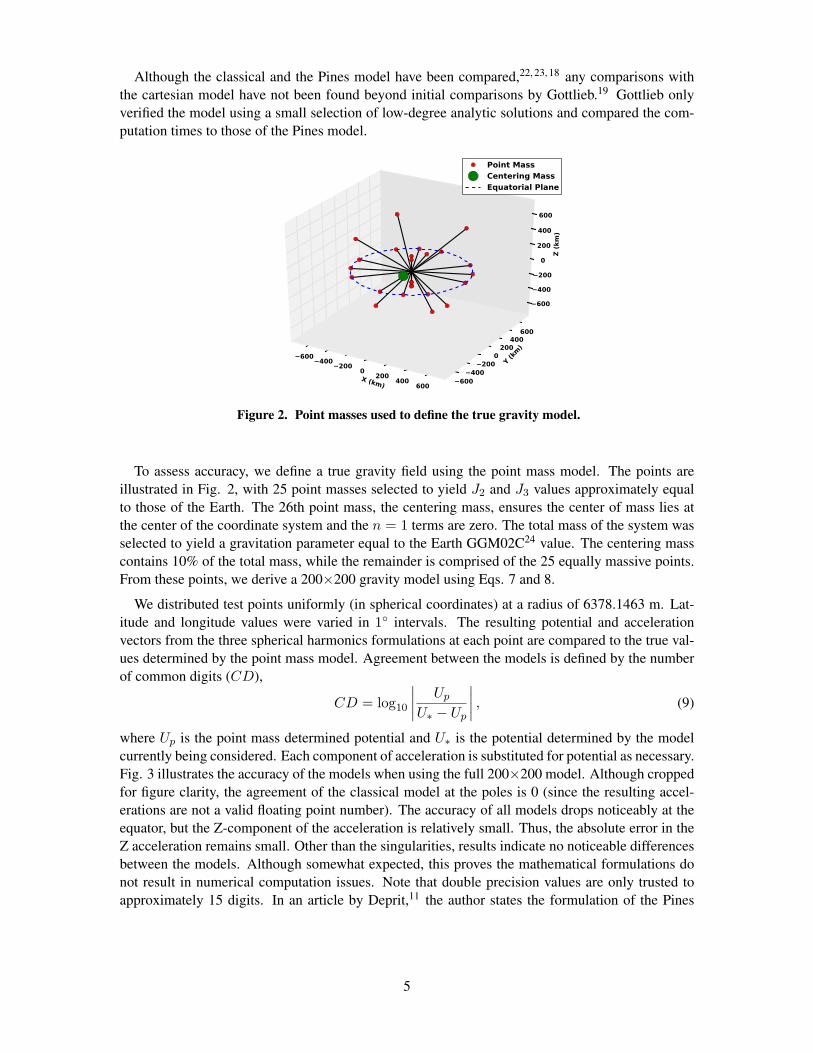
Figure 2. Point masses used to define the true gravity model.

To assess accuracy, we define a true gravity field using the point mass model. The points areillustrated in Fig. 2, with 25 point masses selected to yield J2 and J3 values approximately equalto those of the Earth. The 26th point mass, the centering mass, ensures the center of mass lies atthe center of the coordinate system and the n = 1 terms are zero. The total mass of the system wasselected to yield a gravitation parameter equal to the Earth GGM02C24 value. The centering masscontains 10% of the total mass, while the remainder is comprised of the 25 equally massive points.From these points, we derive a 200×200 gravity model using Eqs. 7 and 8.

We distributed test points uniformly (in spherical coordinates) at a radius of 6378.1463 m. Lat-itude and longitude values were varied in 1◦ intervals. The resulting potential and accelerationvectors from the three spherical harmonics formulations at each point are compared to the true val-ues determined by the point mass model. Agreement between the models is defined by the numberof common digits (CD),

CD = log10

∣∣∣∣ UpU∗ − Up

∣∣∣∣ , (9)

where Up is the point mass determined potential and U∗ is the potential determined by the modelcurrently being considered. Each component of acceleration is substituted for potential as necessary.Fig. 3 illustrates the accuracy of the models when using the full 200×200 model. Although croppedfor figure clarity, the agreement of the classical model at the poles is 0 (since the resulting accel-erations are not a valid floating point number). The accuracy of all models drops noticeably at theequator, but the Z-component of the acceleration is relatively small. Thus, the absolute error in theZ acceleration remains small. Other than the singularities, results indicate no noticeable differencesbetween the models. Although somewhat expected, this proves the mathematical formulations donot result in numerical computation issues. Note that double precision values are only trusted toapproximately 15 digits. In an article by Deprit,11 the author states the formulation of the Pines

5

Figure 3. Average numerical precision, represented as CD, of the potential (U ) andthe components of acceleration for the different formulations of the spherical har-monics model when compared to the true gravity field. Note that the Pines model andClassic model values have been offset by +1 and -1, respectively.

model includes an error for computations at the poles. However, it is unclear if this statement onlyapplies to the variational equations, thus this analysis was further required to clarify the accuracyof the model. We did not consider second derivatives in this study because they are not used in thecubed-shere model.6

0 50 100 150 200Model Degree/Order

0.0

0.2

0.4

0.6

0.8

1.0

1.2

AverageTim

e(m

s)

Average Evaluation Time for 100,000 Executions

Classic

Pines

Cartesian

Cubed Sphere

Figure 4. The figure on the left profiles the average execution time of the cubed sphereand the three spherical harmonics formulations considered as base models. The figureon the right demonstrates the execution time, normalized by the execution time of theclassic model.

A comparison of the average execution time is included in Fig. 4. For lower degree and ordermodels, the classic formulation is slower than the other formulations. We believe this is due to theinitial evaluation of the trigonometric functions used in the recursive formulation of sin(mλ) and

6

cos(mλ). Both the Pines and cartesian models are slower than the classic model for larger degreeand order due to the addition of the fourth partial sum. The cartesian model is faster than the Pinesmodel because the derived Legendre functions of degree n+1 are not evaluated.

Based on these results, we selected the cartesian model as the new base model for the cubed-sphere gravity model. Aside from the polar singularity, there is little difference in the accuracy ofthe mathematical models. Although less computationally efficient than the classical formulationfor degree 20 or greater, the cartesian model eliminates the singularity at the poles. The additionalcomputational burden only impacts the model generation time, which is a one-time cost.

Model Configurations

After the selection of the new base model, we generated new cubed-sphere models. Extendingon previous studies,6 each model generated was optimized to minimize the file size while closelyagreeing with the base model. Specifically, each cubed-sphere model was tuned to exhibit fluctu-ations in the Jacobi-like integration constant25 similar to those of the base model. Cubed-spheremodels based on the 20×20 through 200×200 spherical harmonics models were generated. Theselected values for the grid density and degree of the radial interpolation are provided in Table 1.Note that the naming convention for the cubed-sphere model is CSX where X is the grid densityon the face of the cube, or N/4.

Table 1. Cubed sphere gravity model configurations.

Model Name Base Model Degree/Order Grid Density (N ) Chebyshev Polynomial Degree

CS34 20×20 136 7CS48 30×30 192 8CS62 40×40 248 9CS76 50×50 304 9CS94 60×60 376 9

CS100 70×70 400 10CS112 80×80 448 10CS122 90×90 488 10CS136 100×100 544 10CS148 110×110 592 11CS150 120×120 600 11CS156 130×130 624 11CS164 140×140 656 11CS174 150×150 696 12CS184 160×160 736 12CS192 170×170 768 12

CS198A 180×180 792 12CS198B 190×190 792 12CS198C 200×200 792 12

The speed advantage of the cubed-sphere model, when compared to the spherical harmonics,varies with model degree and order. As seen in Fig. 4, the cubed-sphere model is considerably

7

faster than the spherical harmonics model for high fidelity orbit propagation.

ORBIT DETERMINATION PERFORMANCE

The cubed-sphere model has been integrated with the orbit determination process, although withsome limitations. Most orbit determination methods estimate the error of the expected satellitemotion when compared to the observed motion, which is represented by a deviation vector. Acorrection to the a priori state is then generated based on this deviation vector to more closelymatch the observed motion. Linearized filters, such as the batch least-squares or the Kalman filter,require a state transition matrix (Φ(ti, ti−1)) to map the deviation vector and the estimated filtererror (covariance matrix) through time. Using

Φ = A(X∗, t)Φ, (10)

where A(X∗, t) is the Jacobian of the system dynamics, Φ is numerically integrated along with thereference trajectory. To achieve full accuracy, this Jacobian requires the second derivatives of thegravity potential. These second derivatives are often called the variational equations. Calculationof the variational equations using the cubed-sphere model results in a loss of accuracy.6 Thus,higher degree variations in the gravity field cannot be added to a linearized filter requiring Φ. Twooptions are available for adding the cubed-sphere model to the estimation process: (1) ignore higherdegree perturbations in the Jacobian, or (2) use a non-linear filter. This paper provides results forboth cases. All filter estimated state vectors include the six-component satellite state vector and thecoefficient of drag (CD).

Cubed-Sphere Model Estimation

The number of B-spline interpolation coefficients used to represent the complete cubed-spheremodel my be found using

Number of coefficients = 6p(l + 1)(z − 1)(N

4+ b

)2

, (11)

where p is the number of parameters estimated by the cubed-sphere model, z is the number ofconcentric shells, and other terms have been defined previously. Assuming the model approxi-mates three components of acceleration and has 14 shells, the CS34 model contains 3,790,800coefficients. Estimation of these coefficients via the orbit determination process is an intractableproblem. Current research considers a new model that is formulated for the estimation process.26, 27

Thus, estimation of the gravity field is beyond the scope of this paper.

Filter Implementation

Although considered a non-linear filter, the extended Kalman filter (EKF) requires a linearizedapproximation of the reference trajectory propagation. For implementation of the cubed-spheremodel in the EKF, we propagate the satellite reference trajectory using the full gravity field, butthe variational equations are truncated. Since a small subset of lower degree terms are modeled asspherical harmonics in the cubed-sphere model, implementation in a linearized filter may include thelower degree terms in the evaluation of the Jacobian. This study includes the gravity perturbationdue to J2 in the state transition matrix. For the orbit altitudes considered here, the contributions

8

of the gravity terms of degree three and higher to Φ are small, but are necessary for applicationsdemanding high accuracy.

The cubed sphere has been integrated with a scaled, unscented Kalman filter (UKF);28, 29 a non-linear filter which does not require a Jacobian. Let L equal the number of estimated values inthe filter. Instead of generating Φ, 2L + 1 σ-points are created using the filter covariance matrix.These σ-points are each numerically integrated using the cubed-sphere model, and combined usingthe unscented transformation (UT) to generate a new covariance matrix at the new time. The UTprovides at least a second order propagation of the filter covariance matrix. The scaled UT alwaysyields a positive-definite matrix, which is required of a proper filter algorithm. Thus, the Jacobianof the system is not evaluated, and the variational equations of the gravity field are not required.This also means there are 2L more gravity field evaluations in the integration process at each pointin time.

The UKF computes a weighted average of the observation residuals for each of the filter σ-points,which is then used in the filter measurement update. Given there are 2L+1 state vectors to evaluate,as opposed to one, the UKF requires additional computational resources for each observation.

Filter process noise of the form

Q =

∆t4

4 σ2X

0 0 ∆t3

2 σ2X

0 0

0 ∆t4

4 σ2Y

0 0 ∆t3

2 σ2Y

0

0 0 ∆t4

4 σ2Z

0 0 ∆t3

2 σ2Z

∆t3

2 σ2X

0 0 ∆t2σ2X

0 0

0 ∆t3

2 σ2Y

0 0 ∆t2σ2Y

0

0 0 ∆t3

2 σ2Z

0 0 ∆t2σ2Z

, (12)

where ∆t is the time between measurements, is added to the filter time update of the state-errorcovariance matrix in the UKF. This equation assumes a constant acceleration in each componentdirection for small ∆t and can be derived using Eqs. 4.9.47 and 4.9.50 of Tapley, et al.30 In thisUKF implementation, no process noise is added when ∆t is large. The values of σX , σY , and σZwere determined such that approximately 97.1% of all estimated state errors are within the 3-σ filtercovariance ellipsoid. A single value was determine for each gravity model degree using the filterconfiguration with all errors present. Except where specified, both filters used the same values.

During the coarse of research, we observed the propagation of the estimated state covariancematrix using Φ did not increase the magnitude of the matrix enough to prevent filter saturation.Thus, a phasing factor is applied to the covariance matrix during an observation gap. This phasefactor doubles the estimated state standard deviation every 15 minutes when observations are notavailable. The inclusion of second-order effects when propagating the covariance matrix with theUT appeared to negate the problem in the UKF.

Test Description

We generated “truth” orbits using highly-accurate models of the conservative and nonconserva-tive forces affecting satellite motion. For gravity, the full GGM02C24 200×200 spherical harmonicgravity model is used. The Jacchia-Bowman 2008 (JB2008)31 model provides the most realisticrepresentation of atmospheric density available. Using these models and a prescribed initial state,we propagated the true trajectory of the satellite for observation simulation and filter performance

9

characterization. Numerical integration for both the true trajectories and the filter reference trajec-tories was performed using the TurboProp software package.32 The simulation epoch time of July14, 2000 00:00:00 UTC was selected to correspond with the solar maximum, and thus a higher dragperturbation.

Measurement types considered include Earth-based laser range observations, Earth-based doppler,and satellite-based range. These systems approximate observations from the Satellite Laser Ranging(SLR),33 Doppler Orbitography and Radiopositioning Integrated by Satellite (DORIS),34 and GlobalPositioning System (GPS)35 services, respectively. The locations of the SLR∗ and DORIS† groundstations are based on the actual network. The simulated GPS satellite constellation used the opti-mal 24 satellite design.36 We generated simulated observations using the relative states of the truesatellite trajectory and the measurement reference point, and added Gaussian noise. More accuratemeasurement types are available, such as GPS carrier phase, but they require additional processing.Additionally, the measurement accuracy of the carrier phase measurements tend to yield a reduceddynamic orbit determination system, which reduces the dependency on high-fidelity force models.The goal of this research is to characterize navigation improvements for systems requiring fast orbitdetermination algorithms. Thus, measurement types requiring additional computational resourcesare not considered.

Table 2. Summary of filter error sources. Truth+σ means true value plus zero mean, 1-σ Gaussiannoise. Sigma values are provided where appropriate.

Element Truth Value Filter Value

Initial Position True Position Truth + σ = 1 km errorInitial Velocity True Velocity Truth + σ = 0.5 km/s error

Initial CD 2.3 2.0Gravity Estimate GGM02C 1-σ clone

Gravity Truncation 200×200 Test dependentAtmospheric Density JB2008 NRLMSISE-00

GPS Satellite True Position Truth + periodic error (σ = 5.8 cm)SLR/DORIS Station True Position Truth + σ = 2 cm

A priori and modeling errors were included in the filter to approximate real-world errors seenin the orbit determination problem. These errors are summarized in Table 2. The filter uses theNRLMSISE-00 atmospheric density model,37 which does not incorporate the latest advancementsin space weather modeling. Gaussian noise with zero mean and a standard deviation of 2 cm wasadded to the filter modeled ground station location at filter initialization. The filter modeled GPSsatellite position included a 5.8 cm 1-σ error in each component direction. This corresponds to theestimated 10 cm 3D position prediction error of the IGS ultra-rapid ephemeris.38 To model the 15minute sampling period provided by the IGS solution, the GPS position error is periodic with a2π/15-minute frequency and a random phase offset. The maximum possible measurement bias is10 cm, but the bias never drops to 0 cm.

Gravity errors were introduced to the simulation through model truncation and gravity clones.

∗http://ilrs.gsfc.nasa.gov/stations/index.html, Retrieved August 7, 2008†http://ids.cls.fr/html/doris/network.html, Retrieved August 7, 2008

10

Model truncation varies with the filter test executed. Given

PCSnm= STS, (13)

where S is upper triangular and computed via the Cholesky decomposition, a gravity clone is gen-erated by

Clone = CSnm + S~e (14)

where CSnm is a vector of the Stokes coefficients describing the spherical harmonics gravity model,PCSnm is the full estimation error covariance matrix of the Stokes coefficients, and ~e is a vector ofrandom numbers with zero mean and unit variance. Unfortunately, the GGM02C covariance matrixis not publicly available, so only the diagonal terms could be used in generating the clones. Thus,these are not true clones and are likely a pessimistic representation of the gravity errors. We used fiveof these clones and the original gravity model. Corresponding cubed-sphere models were generatedfor each clone using the configuration of Table 1. Presented results that include gravity clone errorsare an average error for the five clones used in separate filter executions.

Table 3. Observation Noise Properties

Measurement Gaussian Measurement Noise Filter Observation σ

GPS Pseudorange 1 m 1.01 mSLR Range 5 mm 4 cm

DORIS Doppler 2 mm/s 1 cm/s

Observation properties are included in Table 3. The filter observation σ value accounts for errorsin the locations of the GPS satellites and ground stations. Since the measurement reference locationsare not included in the estimated state, the filter must compensate for the station location error. Thefilter observation σ value was selected to yield a normal distribution of prefit-residual errors infilter processing, i.e. the differences between the filter predicted observations and the providedobservations were normally distributed with zero mean and a σ value that is roughly equal to thefilter observation σ value.

Three satellites are simulated for this study: (1) the Gravity Recovery and Climate Experiment(GRACE), (2) Jason-1, and (3) a GPS satellite. The simulated GRACE satellite orbit is nearlycircular at an altitude of 500 km and an inclination of 89◦. The Jason-1 orbit is also circular, but atan altitude of 1336 km and an inclination of 66◦. Finally, the selected GPS satellite orbit is nearlycircular at an altitude of 26,559.8 km, an inclination of 55◦, a right ascension of the ascending nodeof 272.85◦, and an initial true anomaly of 11.68◦. To prevent confusion with the simulated GPSobservation system, we refer to this GPS satellite as the Semi-Synchronous, or SemiSync, satellite.Initial orbital elements not specified here are selected randomly.

Multiple filter configurations were tested for this study. A configuration is defined by the filtererrors present when processing that data. First, the data were processed with all filter error sourcespresent. The error sources were then removed one at a time until only measurement noise wasincluded. For each configuration, the orbit determination performance was characterized for cubed-sphere gravity models of degree 20 through 200. Filter accuracy results are truncated at degree 150since performance for higher degree models match those included. A cubed-sphere model of degree20 indicates a cubed-sphere model derived from a 20×20 spherical harmonics model.

11

Filter Execution Time Results

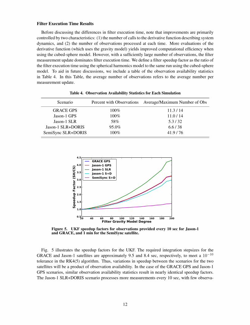
Before discussing the differences in filter execution time, note that improvements are primarilycontrolled by two characteristics: (1) the number of calls to the derivative function describing systemdynamics, and (2) the number of observations processed at each time. More evaluations of thederivative function (which uses the gravity model) yields improved computational efficiency whenusing the cubed-sphere model. However, with a sufficiently large number of observations, the filtermeasurement update dominates filter execution time. We define a filter speedup factor as the ratio ofthe filter execution time using the spherical harmonics model to the same run using the cubed-spheremodel. To aid in future discussions, we include a table of the observation availability statisticsin Table 4. In this Table, the average number of observations refers to the average number permeasurement update.

Table 4. Observation Availability Statistics for Each Simulation

Scenario Percent with Observations Average/Maximum Number of Obs

GRACE GPS 100% 11.3 / 14Jason-1 GPS 100% 11.0 / 14Jason-1 SLR 58% 5.3 / 32

Jason-1 SLR+DORIS 95.0% 6.6 / 38SemiSync SLR+DORIS 100% 41.9 / 76

20 40 60 80 100 120 140 160 180 200Filter Gravity Model Degree

0.5

1.0

1.5

2.0

2.5

3.0

3.5

4.0

4.5

Sp

eed

up

Facto

r (S

H/C

S)

GRACE GPSJason-1 GPSJason-1 SLRJason-1 S+DSemiSync S+D

Figure 5. UKF speedup factors for observations provided every 10 sec for Jason-1and GRACE, and 1 min for the SemiSync satellite.

Fig. 5 illustrates the speedup factors for the UKF. The required integration stepsizes for theGRACE and Jason-1 satellites are approximately 9.5 and 8.4 sec, respectively, to meet a 10−10

tolerance in the RK4(5) algorithm. Thus, variations in speedup between the scenarios for the twosatellites will be a product of observation availability. In the case of the GRACE GPS and Jason-1GPS scenarios, similar observation availability statistics result in nearly identical speedup factors.The Jason-1 SLR+DORIS scenario processes more measurements every 10 sec, with few observa-

12

tion gaps, thus decreasing the speedup factor. In the case of the SLR only scenario for Jason-1, theobservation gaps cause the computation time of the integrator relative to the measurement updateto increase. The contribution of integration to the total execution time increases, and the speedupfactor increases. In the case of the SemiSync scenario, the large number of observations dominatethe speedup factor. Hence, little improvement is attained for this case. Models of degree 190 exhibita larger than expected speedup factor, when considering the dominating trend. Although somewhatanomalous, this event was repeatable and consistent between tests.

1.00

1.01

1.02

1.03

1.04

1.05

Cu

bed

Sp

here

GRACE GPSJason-1 GPSJason-1 SLR

Jason-1 S+DSemiSync S+D

20 40 60 80 100 120 140 160 180 200Filter Gravity Model Degree

1.0

1.5

2.0

2.5

3.0

3.5

4.0

4.5

5.0

Sp

h.

Harm

on

ic

Figure 6. UKF Normalized Execution Time.

We provide the filter execution time, normalized to the execution time of the 20×20 model, inFig. 6. For the cubed-sphere model, eleventh degree B-splines are used for all models. Thus, themain parameter causing an increase in computation time is the degree of the Chebyshev interpola-tion in the radial direction, which increases with base model degree. The increased file size alsoincreases evaluation time when accessing the model in memory. The cubed-sphere-model-filterexecution time only increases by 4%, whereas the spherical-harmonic-model filter increases by asmuch as 350%. Fig. 6 indicates the anomaly in the speedup factors, as seen in Fig. 5, is causedby the evaluation time of the 190x190 spherical harmonic gravity model. The cause for this is notknown at this time.

In Fig. 7, we provide the speedup factors for the EKF. The cubed-sphere model EKF run iscompared to a similar run with the spherical harmonics to propagate the reference trajectory and onthe J2 term included in the Jacobian. The EKF only propagates one estimated state vector. Thus,the speedup factors decrease with the reduced number of gravity model evaluations. The reductionin the time required for measurement processing partially offsets this decrease. The observationgaps present in the SLR+DORIS scenario increase the impact of the integration time on the execu-tion time, thus this scenario is faster than the GPS observation simulations. Otherwise, results areconsistent with those of Fig. 5.

13

20 40 60 80 100 120 140 160 180 200Filter Gravity Model Degree

0.5

1.0

1.5

2.0

2.5

3.0

3.5

4.0

4.5

Sp

eed

up

Facto

r (S

H/C

S)

GRACE GPSJason-1 GPSJason-1 SLRJason-1 S+DSemiSync S+D

Figure 7. EKF speedup factors (ratio of spherical harmonics model execution time tothe cubed-sphere model).

20 40 60 80 100 120 140 160 180 200Filter Gravity Model Degree

0

2

4

6

8

10

12

14

16

Sp

eed

up

Facto

r (S

H/C

S)

1 sec10 sec30 sec5 minutes

20 40 60 80 100 120 140 160 180 200Filter Gravity Model Degree

1.0

1.5

2.0

2.5

3.0

Sp

eed

up

Facto

r (S

H/C

S)

1 sec10 sec30 sec5 minutes

Figure 8. Speedup factors for the Jason-1 satellite using GPS observations providedat different intervals. The plot on the right has a reduced scale to see small differencesbetween the 1 s and 10 s scenarios.

14

The Jason-1 navigation team processes GPS normal points every 5 minutes∗. However, they areconsidering a switch to every 30 sec. Fig. 8 compares the speedup factor for the Jason-1 satellite,using GPS observations, at these longer measurement intervals. Additionally, as a comparison,we process the observations at a 1 sec interval. With the increased integration time for the longerintervals, the speedup factor increases up to 15. When processing observations at 1 sec, there islittle change in the speedup factor when compared to the 10 sec scenario. For a 1 sec observationinterval, the observation frequency drives the number of calls to the derivative function. Since therequired integration stepsize is approximately 10 sec, the number of calls to the derivative functionper time update remains constant at or below a 10 sec measurement interval. Since the ratio ofintegration time and measurements processed does not change, the speedup factor only increasesfor observation intervals greater than 10 sec.

Filter Accuracy Results

This section presents accuracy performance of the tests previously described when using thecubed-sphere gravity model. We do not include comparisons of the filter solutions using the cubed-sphere model to those using the spherical harmonics. Since the cubed-sphere model is tuned toclosely agree with the spherical harmonics model, filter estimated states are nearly identical. Addi-tionally, accuracy improvements for the SemiSync satellites are not included here. Given the largealtitude, no improvement is exhibited for higher degree models.

We verified the proper tuning of the filter process noise by comparing the filter estimated 1-σ error to the actual filter 1-σ error for the scenarios including all model discrepancies. Valueswere approximately equal, implying measurement noise accounts for the demonstrated filter errors.Further changes in process noise will not necessarily improve filter accuracy.

Figure 9. 3D RMS filter performance for the GRACE orbit using GPS pseudorange measurements.

Fig. 9 illustrates the results for the GRACE satellite orbit using pseudorange measurements. Notethat errors decrease with increased gravity model degree until around degree 80. This indicates theprinciple source of estimation error using the low-degree models is gravity truncation. In position,

∗Personal communciation with Shailen Desai of the NASA Jet Propulsion Laboratory

15

the filter performance improves by as much as a factor of 2 when using a cubed-sphere model ofdegree 80 or higher. Velocity errors are reduced by an order of magnitude. Differences in errorbetween the scenarios would be visible with increased measurement accuracy.

GPS pseudorange filter performance for the Jason-1 satellite is provided in Fig. 10. Using gravitymodels of degree higher than 50 do not improve filter performance, and degree 50 is only a slightimprovement over degree 40. The reduced threshold for filter improvement with increased gravitymodel degree is a result of attenuation of the higher-degree gravity terms at the higher Jason-1 orbitaltitude.

Figure 10. 3D RMS filter performance for the Jason-1 orbit using GPS pseudorange measurements.

In Fig. 10, the measurement noise only case did not necessarily exhibit the best performance. Weremind the reader that process noise values were selected based on the scenarios with all modelingerrors present, and the same process noise σ values were used for all filter configurations. Processnoise compensates for unknown modeling errors, but the measurement only scenario did not containany modeling errors other than gravity model truncation. When process noise is applied to a filterwith small modeling errors, it causes the filter to weight the observations higher than the predictedsatellite motion, which can adversely affect filter performance. These results are an example of thisfact.

Filter results using ground-based observations, both SLR and DORIS, are included in Fig. 11.Like the Jason-1 GPS results, the filter continues to improve as the gravity model degree is increasedup to 40. In order to prevent filter saturation for the EKF, we increased the process noise σ values,which slightly reduced performance. Otherwise, the EKF diverged or took an excessively longtime to converge on an accurate solution. The UKF did not require this larger σ value because theunscented transformation provides second (and possibly third) order propagation of the covariancematrix.

For each scenario, we processed three configurations of the EKF. The first configuration used thecubed-sphere gravity model with only J2 in the Jacobian. The second configuration substituted thespherical harmonics model for the cubed-sphere model. The third configuration used the sphericalharmonics model with the full variational equations (up to the filter specified filter gravity modeldegree). We compared the filter performance of the EKF for all three configurations, with little

16

Figure 11. 3D RMS filter performance for the Jason-1 orbit using SLR and DORIS measurements.

difference exhibited. Since the truncated terms are only a small contribution to the Jacobian, filterperformances are nearly identical. Results are not included here in the interest of brevity. Differ-ences in the filters should be increased with more accurate measurements.

CONCLUSIONS

This paper describes initial studies to characterize potential filter improvements using the cubed-sphere gravity model. For the scenarios tested, results demonstrate a higher degree gravity modelmay be integrated with the orbit determination process with little increase in execution time. Thisresults in increased accuracy by reducing gravity truncation error. Based on the satellite orbit alti-tude, benefits are reduced above a given gravity model degree.

Results indicate the largest execution time improvements occur for scenarios with longer obser-vation gaps and fewer observations. Although the filter execution time required when using thecubed-sphere gravity model increases for higher degree models, the increase is less than 5% for a200×200 versus a 20×20 model.

Several future studies are required to fully characterize the filter improvements. This paper de-scribed tests for two satellites at roughly 500 and 1300 km in altitude. A more detailed profile of theorbit altitudes from 250 km up to 1400 km is required. A study of filter prediction accuracy whenusing a higher degree gravity model may also be interesting for autonomous navigation during orwhen reacquiring a satellite after an observation gap.

It would also be interesting to characterize changes in filter performance when there are largergaps between observation passes. For example, SLR monitoring of a low-Earth orbiter. Given therelatively small number of ground stations, a satellite at lower altitudes will quickly pass over a laserground station, with larger delays between passes. Although such a test would not benefit real-timenavigation, it would benefit space surveillance systems where measurements are limited and manyobjects are tracked.

The execution time of the cubed-sphere gravity model may be slightly decreased when multires-olution techniques are used. Such techniques result in a coarser grid on the surface of the cube, and

17

decrease the precision of the cubed sphere with the base model. In the case of a spherical harmonicsbase model, this process is analagous to smoothing the higher degree terms. Previous studies soughtto create models that closely agree with the spherical harmonics model, given the gravity knowl-edge of the Earth is relatively mature. However, this study demonstrates the higher degree terms donot influence the estimated filter state, and multiresolution techniques may further reduce the filterprocessing time without affecting filter accuracy.

ACKNOWLEDGMENTS

A majority of this research was funded by the NASA Graduate Student Researchers Program(NASA/GSRP) through the Johnson Space Center. Gregory Beylkin’s research is supported byAFOSR grant FA9550-07-1-0135.

NOTATION

U geopotentialr instantaneous orbit radiusφ geocentric latitudeλ longitudeµ gravitation parametern spherical harmonic degreem spherical harmonic order

Pn,m normalized associated Legendre polynomial of degree n and order mCn,m, Sn,m normalized Stokes coefficients

~a acceleration vectorux unit vector in the x directionN cubed-sphere model grid sizeb B-spline interpolation degreel Chebyshev interpolation degreez Number of cubed sphere concentric shellsp Number of values estimated by the cubed sphere

Rp point mass model radiusUp point mass determined gravity potentialηi mass of i-th point mass~Rp point mass positionM total mass of point mass systemG gravitation constant~rr point mass model acceleration

CD number of common digitsσx standard deviation of variable x

CSnm Stokes coefficients, arranged as a vectorPCSN,m

variance-covariance matrix of the estimated Stokes coefficients~e vector of random numbersΦ filter state transition matrixA Jacobian matrix of filter dynamical equationsL number of filter estimated states

18

REFERENCES[1] C. Rocken, Y.-H. Kuo, W. S. Schreiner, D. Hunt, S. Sokolovskiy, and C. McCormick, “COSMIC System

Description,” Terrestrial, Atmospheric and Oceanic Science, Vol. 11, March 2000, pp. 21–52.[2] L. D. James, “Keeping the Space Environment Safe for Civil and Commercial Users,” Testimony to

the Subcommittee on Space and Aeronautics, House Committee on Science and Technology, 28 April2009.

[3] B. Haines, W. I. Bertiger, S. Desai, D. Kuang, T. Munson, L. Young, and P. Willis, “Initial OrbitDetermination Results for Jason-1: Towards a 1 cm Orbit,” Navigation: Journal of the Institute ofNavigation, Vol. 50, Fall 2003.

[4] M. Ablain, A. Cazenave, G. Valladeau, and S. Guinehut, “A New Assessment of the Error Budget ofGlobal Mean Sea Level Rate Estimated by Satellite Altimetry Over 1993-2008,” Ocean Science, Vol. 5,June 2009, pp. 193–201.

[5] G. Beylkin and R. Cramer, “Toward Multiresolution Estimation and Efficient Representation of Gravi-tational Fields,” Celestial Mechanics and Dynamical Astronomy, Vol. 84, 2002, pp. 87–104.

[6] B. A. Jones, G. H. Born, and G. Beylkin, “Comparisons of the Cubed-Sphere Gravity Model with theSpherical Harmonics,” Journal of Guidance, Control, and Dynamics, Vol. 33, March-April 2010.

[7] J. L. Junkins, “Investigation of Finite-Element Representations of the Geopotential,” AIAA Journal,Vol. 14, June 1976, pp. 803–808.

[8] R. C. Engels and J. L. Junkins, “Local Representation of the Geopotential by Weighted OrthonormalPolynomials,” Journal of Guidance and Control, Vol. 3, Jan.-Feb. 1980, pp. 55–61.

[9] A. Colombi, A. N. Hirani, and B. F. Villac, “Adaptive Gravitational Force Representation for FastTrajectory Propagation Near Small Bodies,” Journal of Guidance, Control, and Dynamics, Vol. 31,July-August 2008, pp. 1041–1051.

[10] A. Colombi, A. N. Hirani, and B. F. Villac, “Structure Preserving Approximations of ConservativeForces for Application to Small Body Dynamics,” Journal of Guidance, Control, and Dynamics, Vol. 32,November - December 2009, pp. 1847–1858.

[11] A. Deprit, “Note on the Summation of Legendre Series,” Celestial Mechanics, Vol. 20, No. 4, 1979,pp. 319–323.

[12] L. E. Cunningham, “On the Computation of the Spherical Harmonic Terms Needed During the Numeri-cal Integration of the Orbital Motion of an Artificial Satellite,” Celestial Mechanics, Vol. 2, No. 2, 1970,pp. 207–216.

[13] C. C. Tscherning, R. H. Rapp, and C. Goad, “A Comparison of Methods for Computing GravimetricQuantities from High Degree Spherical Harmonic Expansions,” Manuscripta Geodectica, Vol. 8, 1983,pp. 249–272.

[14] P. J. Melvin, “Comments on the Summations of Spherical Harmonics in the Geopotential EvaluationTheories of Deprit and Others,” Celestial Mechanics and Dynamical Astronomy, Vol. 35, April 1985,pp. 345–355.

[15] S. Pines, “Uniform Representation of the Gravitational Potential and its Derivatives,” AIAA Journal,Vol. 11, Nov. 1973, pp. 1508–1511.

[16] J. L. Spencer, “Pines’ Nonsingular Gravitational Potential Derivation, Description and Implementation,”Tech. Rep. NASA Contractor Report 147478, NASA Lyndon B. Johnson Space Center, Houston, TX,February 1976.

[17] J. B. Lundberg and B. E. Schutz, “Recursion Formulas of Legendre Functions for Use with NonsingularGeopotential Models,” Journal of Guidance, Vol. 11, Jan.-Feb. 1988, pp. 31–38.

[18] E. Fantino and S. Casotto, “Methods of Harmonic Synthesis for Global Geopotential Models and TheirFirst-, Second-, and Third-order Gradients,” Journal of Geodesy, Vol. 83, November 2009, pp. 595–619.

[19] R. G. Gottlieb, “Fast Gravity, Gravity Partials, Normalized Gravity, Gravity Gradient Torque and Mag-netic Field: Derivation, Code and Data,” Tech. Rep. NASA Contractor Report 188243, NASA LyndonB. Johnson Space Center, Houston, TX, February 1993.

[20] P. J. Mohr, B. N. Taylor, and D. B. Newell, “CODATA Recommended Values of the FundamentalPhysical Constants: 2006,” tech. rep., National Institute of Standards and Technology, Gaithersburg,Maryland, 20899, USA, December 2007.

[21] B. F. Thompson, D. G. Hammen, A. A. Jackson, and E. Z. Crues, “Validation of Gravity Accelerationand Torque Algorithms for Astrodynamics,” 18th Annual AAS/AIAA Spaceflight Mechanics Meeting,Galveston, Texas, January 28 - 31 2008.

[22] S. V. Bettadpur, “Hotine’s Geopotential Formulation: Revisited,” Bulletin Geodesique, Vol. 69, Septem-ber 1995, pp. 135–142.

19

[23] S. Casotto and E. Fantino, “Evaluation of methods for spherical harmonic synthesis of the gravitationalpotential and its gradients,” Advances in Space Research, Vol. 40, 2007, pp. 69–75.

[24] B. Tapley, J. Ries, S. Bettadpur, D. Chambers, M. Cheng, F. Condi, B. Gunter, Z. Kang, P. Nagel,R. Pastor, T. Pekker, S. Poole, and F. Wang, “GGM02 - An Improved Earth Gravity Field Model fromGRACE,” Journal of Geodesy, Vol. 79, 2005, pp. 467–478.

[25] V. R. Bond and M. C. Allman, Modern Astrodynamics. Princeton, New Jersey: Princeton UniversityPress, 1996.

[26] C. Ahrens and G. Beylkin, “Rotationally Invariant Quadratures for the Sphere,” Proceedings of theRoyal Society A, Vol. 465, October 2009, pp. 3103–3125.

[27] G. Beylkin and L. Monzon, “Approximation by Exponential Sums Revisited,” Applied ComputationalHarmonic Analysis, Accepted, http://ds.doi.org/10.1016/j.acha.2009.08.011, 2009.

[28] S. J. Julier and J. K. Uhlmann, “A New Extension of the Kalman Filter to Nonlinear Systems,” Proceed-ings of SPIE, Vol. 3068, 1997, pp. 182–193.

[29] S. J. Julier, “The Scaled Unscented Transformation,” Proceedings of the IEEE American Control Con-ference, Anchorage, Alaska, IEEE, May 8-10, 2002 2002, pp. 4555–4559.

[30] B. D. Tapley, B. E. Schutz, and G. H. Born, Statistical Orbit Determination. Burlington, MA: ElsevierAcademic Press, first ed., 2004.

[31] B. R. Bowman, W. K. Tobiska, F. A. Marcos, C. Y. Huang, C. S. Lin, and W. J. Burke, “A New Em-pirical Thermospheric Density Model JB2008 Using New Solar and Geomagnetic Indices,” AIAA/AASAstrodynamics Specialist Conference, Honolulu, Hawaii, August 18-21 2008.

[32] K. Hill and B. A. Jones, TurboProp Version 4.0. Colorado Center for Astrodynamics Research, May2009.

[33] M. R. Pearlman, J. J. Degnan, and J. M. Bosworth, “The International Laser Ranging Service,” Advancesin Space Research, Vol. 30, July 2002, pp. 135–143.

[34] G. Tavernier, H. Fagard, M. Feissel-Vernier, K. LeBail, F. G. Lemoine, C. Noll, R. Noomen, J. C.Ries, L. Soudarin, J.-J. Valette, and P. Willis, “The International DORIS Service: Genesis and EarlyAchievements,” Journal of Geodesy, Vol. 80, November 2006, pp. 403–417.

[35] Navstar GPS Joint Program Office, Navstar GPS Space Segment/Navigation User Interfaces (IS-GPS-200D), revision d ed., December 7 2004.

[36] P. Massatt and M. Zeitzew, “The GPS Constallation Design - Current and Projected,” Proceedings ofthe National Techincal Meeting, Institute of Navigation, January 21-23 1998, pp. 435–445.

[37] J. M. Picone, A. E. Hedin, and D. P. Drob, “NRLMSISE-00 Empirical Model of the Atmosphere:Statistical Comparisons and Scientific Issues,” Journal of Geophysical Research, Vol. 107, No. A12,2002, pp. 1–16.

[38] J. M. Dow, R. E. Neilan, and C. Rizos, “The International GNSS Service In a Changing Landscape ofGlobal Navigation Satellite Systems,” Journal of Geodesy, Vol. 83, 2009, pp. 191–198.

20