general background on computing
TRANSCRIPT
General Background on Computing
Mika Hirvensalo
Department of Mathematics and StatisticsUniversity of Turku
Thessaloniki, May 2016
Mika Hirvensalo General Background on Computing 1 of 68

About Turku
Established 13rd century, capital of Finland until 1812Population 186 000 (city area) 320 000 (subregion area)
Mika Hirvensalo General Background on Computing 2 of 68

About Turku
Established 13rd century
, capital of Finland until 1812Population 186 000 (city area) 320 000 (subregion area)
Mika Hirvensalo General Background on Computing 2 of 68

About Turku
Established 13rd century, capital of Finland until 1812
Population 186 000 (city area) 320 000 (subregion area)
Mika Hirvensalo General Background on Computing 2 of 68

About Turku
Established 13rd century, capital of Finland until 1812Population 186 000 (city area) 320 000 (subregion area)
Mika Hirvensalo General Background on Computing 2 of 68

About Turku
Mika Hirvensalo General Background on Computing 3 of 68

About Turku
Mika Hirvensalo General Background on Computing 3 of 68

About Turku
Mika Hirvensalo General Background on Computing 3 of 68

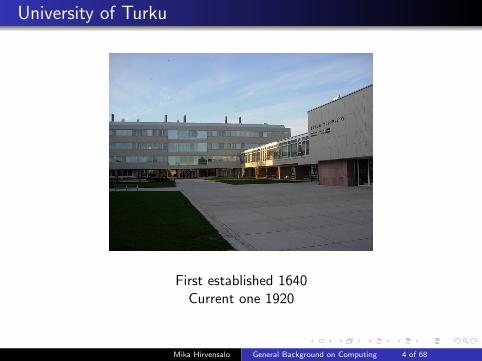
University of Turku
First established 1640
Current one 192020 000 students in seven faculties
Mika Hirvensalo General Background on Computing 4 of 68
University of Turku
First established 1640Current one 1920
20 000 students in seven faculties
Mika Hirvensalo General Background on Computing 4 of 68

University of Turku
First established 1640Current one 1920
20 000 students in seven faculties
Mika Hirvensalo General Background on Computing 4 of 68

Department of Mathematics and Statistics
Discrete mathematics:
Coding Theory and CryptographyComplex Systems and ComputingNumber TheoryWords and Automata
Analysis
Functional analysisGeometric complex analysis
Applied Mathematics
BiomathematicsOptimization
Statistics
Analysis methods for e.g. cancer cell data
Mika Hirvensalo General Background on Computing 5 of 68
Terminology
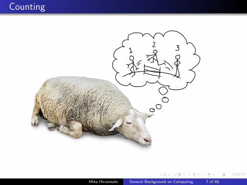
Counting: Recognizing, estimating or determining the number ofobjects
Computing: Rewriting data represented with finitely manysymbols, using a set of finitely specified local rules
Elementary computational step: One application of a local rule.
Mika Hirvensalo General Background on Computing 6 of 68

Terminology
Counting: Recognizing, estimating or determining the number ofobjects
Computing: Rewriting data represented with finitely manysymbols, using a set of finitely specified local rules
Elementary computational step: One application of a local rule.
Mika Hirvensalo General Background on Computing 6 of 68
Counting
Mika Hirvensalo General Background on Computing 7 of 68
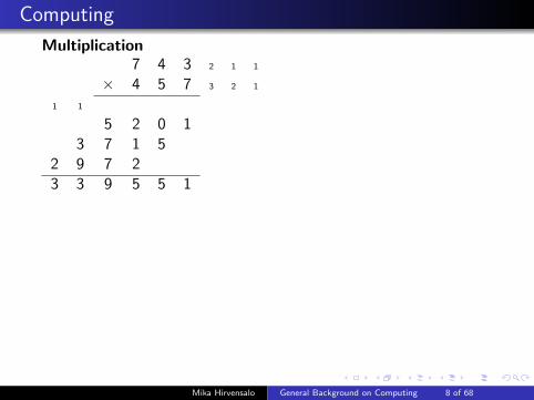
Computing
Multiplication7 4 3 2 1 1
× 4 5 7 3 2 1
1 1
5 2 0 13 7 1 5
2 9 7 23 3 9 5 5 1
Addition1 1
2 9 9+ 1
3 0 0
Elementary steps: Eg. Single-digit multiplication and addition
Mika Hirvensalo General Background on Computing 8 of 68

Computing
Multiplication7 4 3 2 1 1
× 4 5 7 3 2 1
1 1
5 2 0 13 7 1 5
2 9 7 23 3 9 5 5 1
Addition1 1
2 9 9+ 1
3 0 0
Elementary steps: Eg. Single-digit multiplication and addition
Mika Hirvensalo General Background on Computing 8 of 68

Computing
Multiplication7 4 3 2 1 1
× 4 5 7 3 2 1
1 1
5 2 0 13 7 1 5
2 9 7 23 3 9 5 5 1
Addition1 1
2 9 9+ 1
3 0 0
Elementary steps: Eg. Single-digit multiplication and addition
Mika Hirvensalo General Background on Computing 8 of 68

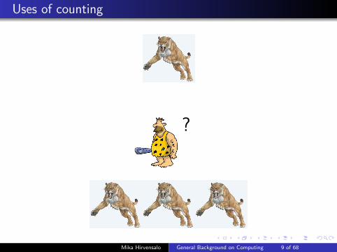
Uses of counting
?
Mika Hirvensalo General Background on Computing 9 of 68
Uses of counting
?
Mika Hirvensalo General Background on Computing 9 of 68
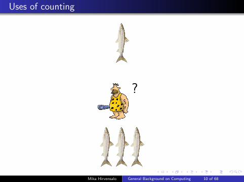
Uses of counting
?
Mika Hirvensalo General Background on Computing 10 of 68
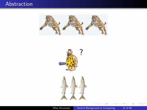
Abstraction
?
Mika Hirvensalo General Background on Computing 11 of 68

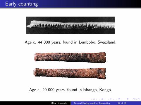
Early counting
Age c. 44 000 years, found in Lembobo, Swaziland.
Age c. 20 000 years, found in Ishango, Kongo.
Mika Hirvensalo General Background on Computing 12 of 68
Early counting
Age c. 44 000 years, found in Lembobo, Swaziland.
Age c. 20 000 years, found in Ishango, Kongo.
Mika Hirvensalo General Background on Computing 12 of 68

From counting to computing
Babylonian multiplication table, approx. 3700–3900 years ago.
Mika Hirvensalo General Background on Computing 13 of 68

Uses of computing: Trading
=
+ ?
Mika Hirvensalo General Background on Computing 14 of 68

Beyond counting and computing
Mika Hirvensalo General Background on Computing 15 of 68

Beyond counting and computing
Rhind papyrus, approx. 3600 years ago.
Mika Hirvensalo General Background on Computing 16 of 68

Mechanical computing
Antikythera machine, approx. 2200 years ago.
Mika Hirvensalo General Background on Computing 17 of 68

Mechanical computing
Antikythera machine, approx. 2200 years ago.
Mika Hirvensalo General Background on Computing 17 of 68

Mechanical computing
A modern reconstruction of the Antikythera machine: Solar systemcalender
Mika Hirvensalo General Background on Computing 18 of 68

Mechanical computing
Roman abacus (replica), approx. 1800 years ago.
Mika Hirvensalo General Background on Computing 19 of 68

Mechanical computing: bibliography
Oxford University Press (2013)
Mika Hirvensalo General Background on Computing 20 of 68

Mechanical computing with electronic aid
Friden calculator (1949 –1966)
Mika Hirvensalo General Background on Computing 21 of 68
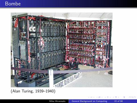
Bombe
(Alan Turing, 1939–1940)
Mika Hirvensalo General Background on Computing 22 of 68

Electronic computing
Colossus Mark 2 (1944) (to analyze the Lorenz chiper)
Mika Hirvensalo General Background on Computing 23 of 68

Semiconductor technology
Commodore 64 (1982–1993) 1 MHz, 64 kB RAM
Mika Hirvensalo General Background on Computing 24 of 68

Semiconductor technology
ASUS ZenBook UX305FA (2015–) 0.8–2 GHz Dual core, 8 GBRAM + 256 GB SSD
Mika Hirvensalo General Background on Computing 25 of 68

Moore’s law
Mika Hirvensalo General Background on Computing 26 of 68

Programmable computers
Hardware + software
Hardware provides a physical platform for processing data(“body”)
Software encodes the rules of data processing (“soul”)
Mika Hirvensalo General Background on Computing 27 of 68
Programmable computers
Hardware + software
Hardware provides a physical platform for processing data(“body”)
Software encodes the rules of data processing (“soul”)
Mika Hirvensalo General Background on Computing 27 of 68
Programmable computers
Hardware + software
Hardware provides a physical platform for processing data(“body”)
Software encodes the rules of data processing (“soul”)
Mika Hirvensalo General Background on Computing 27 of 68
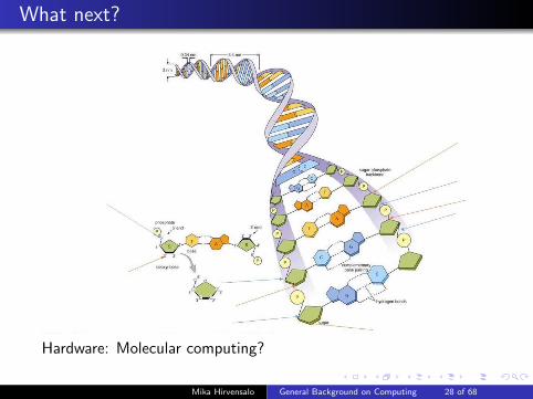
What next?
Hardware: Molecular computing?
Mika Hirvensalo General Background on Computing 28 of 68

What next?
Software: Intelligence?
Mika Hirvensalo General Background on Computing 29 of 68
What next?
Awareness, human intelligence?
Mika Hirvensalo General Background on Computing 30 of 68
What next?
Superhuman intelligence?
Mika Hirvensalo General Background on Computing 31 of 68
Encyclopædia Britannica:
Computer, device for processing, storing, and displayinginformation.Computer once meant a person who did computations, but now theterm almost universally refers to automated electronic machinery.
Mika Hirvensalo General Background on Computing 32 of 68
Computational problems
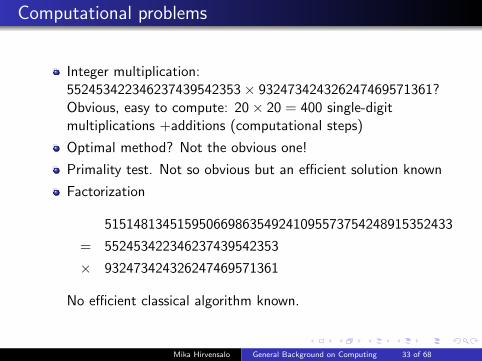
Integer multiplication:552453422346237439542353× 932473424326247469571361?
Obvious, easy to compute: 20× 20 = 400 single-digitmultiplications +additions (computational steps)
Optimal method? Not the obvious one!
Primality test. Not so obvious but an efficient solution known
Factorization
515148134515950669863549241095573754248915352433
= 552453422346237439542353
× 932473424326247469571361
No efficient classical algorithm known.
Mika Hirvensalo General Background on Computing 33 of 68

Computational problems
Integer multiplication:552453422346237439542353× 932473424326247469571361?Obvious, easy to compute: 20× 20 = 400 single-digitmultiplications +additions (computational steps)
Optimal method?
Not the obvious one!
Primality test. Not so obvious but an efficient solution known
Factorization
515148134515950669863549241095573754248915352433
= 552453422346237439542353
× 932473424326247469571361
No efficient classical algorithm known.
Mika Hirvensalo General Background on Computing 33 of 68

Computational problems
Integer multiplication:552453422346237439542353× 932473424326247469571361?Obvious, easy to compute: 20× 20 = 400 single-digitmultiplications +additions (computational steps)
Optimal method? Not the obvious one!
Primality test. Not so obvious but an efficient solution known
Factorization
515148134515950669863549241095573754248915352433
= 552453422346237439542353
× 932473424326247469571361
No efficient classical algorithm known.
Mika Hirvensalo General Background on Computing 33 of 68

Computational problems
Integer multiplication:552453422346237439542353× 932473424326247469571361?Obvious, easy to compute: 20× 20 = 400 single-digitmultiplications +additions (computational steps)
Optimal method? Not the obvious one!
Primality test. Not so obvious but an efficient solution known
Factorization
515148134515950669863549241095573754248915352433
= 552453422346237439542353
× 932473424326247469571361
No efficient classical algorithm known.
Mika Hirvensalo General Background on Computing 33 of 68

Computational problems
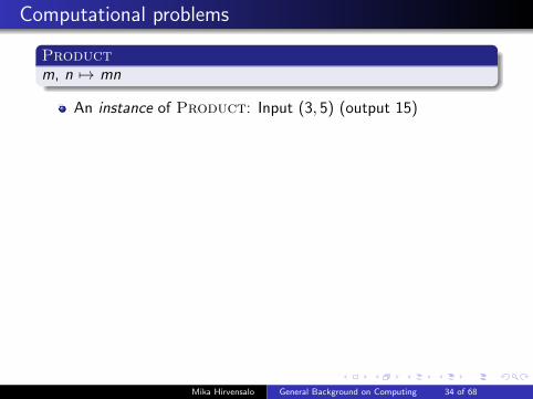
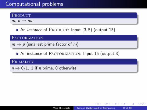
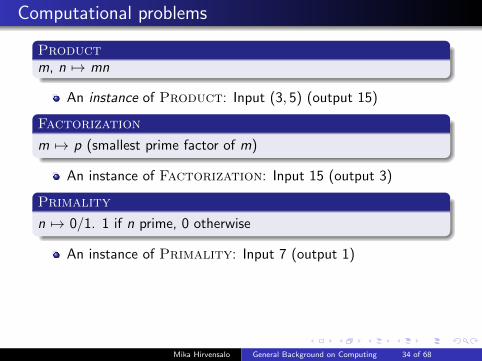
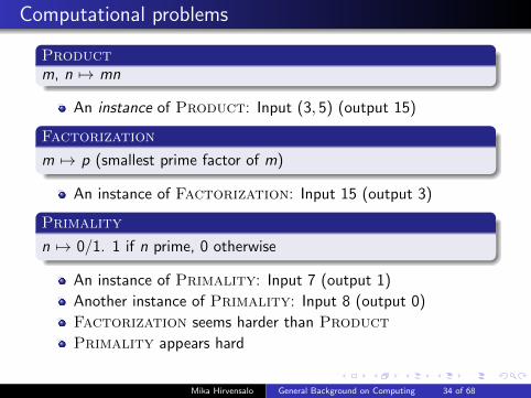
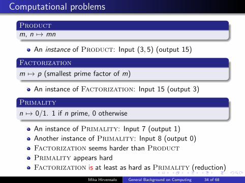
Productm, n 7→ mn
An instance of Product: Input (3, 5) (output 15)
Factorization
m 7→ p (smallest prime factor of m)
An instance of Factorization: Input 15 (output 3)
Primality
n 7→ 0/1. 1 if n prime, 0 otherwise
An instance of Primality: Input 7 (output 1)
Another instance of Primality: Input 8 (output 0)
Factorization seems harder than Product
Primality appears hard
Factorization is at least as hard as Primality (reduction)
Mika Hirvensalo General Background on Computing 34 of 68

Computational problems
Productm, n 7→ mn
An instance of Product: Input (3, 5) (output 15)
Factorization
m 7→ p (smallest prime factor of m)
An instance of Factorization: Input 15 (output 3)
Primality
n 7→ 0/1. 1 if n prime, 0 otherwise
An instance of Primality: Input 7 (output 1)
Another instance of Primality: Input 8 (output 0)
Factorization seems harder than Product
Primality appears hard
Factorization is at least as hard as Primality (reduction)
Mika Hirvensalo General Background on Computing 34 of 68
Computational problems
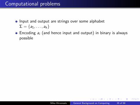
Input and output are strings over some alphabetΣ = {a1, . . . , ak}
Encoding ai (and hence input and output) in binary is alwayspossible
Decision problems: Output ∈ {0, 1}
A general problem can be presented as a sequence of decisionproblems: 1:st bit of the output? 2:nd bit of the output? etc.
Computation: InputA−→ Output
What does it take to compute A? How much time? Howmuch space?
Mika Hirvensalo General Background on Computing 35 of 68
Computational problems
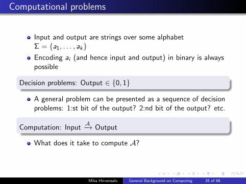
Input and output are strings over some alphabetΣ = {a1, . . . , ak}Encoding ai (and hence input and output) in binary is alwayspossible
Decision problems: Output ∈ {0, 1}
A general problem can be presented as a sequence of decisionproblems: 1:st bit of the output? 2:nd bit of the output? etc.
Computation: InputA−→ Output
What does it take to compute A? How much time? Howmuch space?
Mika Hirvensalo General Background on Computing 35 of 68

Computational problems
Input and output are strings over some alphabetΣ = {a1, . . . , ak}Encoding ai (and hence input and output) in binary is alwayspossible
Decision problems: Output ∈ {0, 1}
A general problem can be presented as a sequence of decisionproblems: 1:st bit of the output? 2:nd bit of the output? etc.
Computation: InputA−→ Output
What does it take to compute A? How much time? Howmuch space?
Mika Hirvensalo General Background on Computing 35 of 68
Computational problems
Input and output are strings over some alphabetΣ = {a1, . . . , ak}Encoding ai (and hence input and output) in binary is alwayspossible
Decision problems: Output ∈ {0, 1}
A general problem can be presented as a sequence of decisionproblems: 1:st bit of the output? 2:nd bit of the output? etc.
Computation: InputA−→ Output
What does it take to compute A?
How much time? Howmuch space?
Mika Hirvensalo General Background on Computing 35 of 68
Computational problems
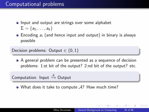
Input and output are strings over some alphabetΣ = {a1, . . . , ak}Encoding ai (and hence input and output) in binary is alwayspossible
Decision problems: Output ∈ {0, 1}
A general problem can be presented as a sequence of decisionproblems: 1:st bit of the output? 2:nd bit of the output? etc.
Computation: InputA−→ Output
What does it take to compute A? How much time?
Howmuch space?
Mika Hirvensalo General Background on Computing 35 of 68
Computational problems
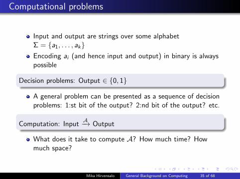
Input and output are strings over some alphabetΣ = {a1, . . . , ak}Encoding ai (and hence input and output) in binary is alwayspossible
Decision problems: Output ∈ {0, 1}
A general problem can be presented as a sequence of decisionproblems: 1:st bit of the output? 2:nd bit of the output? etc.
Computation: InputA−→ Output
What does it take to compute A? How much time? Howmuch space?
Mika Hirvensalo General Background on Computing 35 of 68

Computational Complexity – Preliminaries
What is computation?
How to measure the complexity of computation?
Time / Space ? Physical time (in seconds) not useful
Mika Hirvensalo General Background on Computing 36 of 68
Computational Complexity – Preliminaries
What is computation?
How to measure the complexity of computation?
Time / Space ? Physical time (in seconds) not useful
Mika Hirvensalo General Background on Computing 36 of 68

Computational Complexity – Preliminaries
What is computation?
How to measure the complexity of computation?
Time / Space ?
Physical time (in seconds) not useful
Mika Hirvensalo General Background on Computing 36 of 68

Computational Complexity – Preliminaries
What is computation?
How to measure the complexity of computation?
Time / Space ? Physical time (in seconds) not useful
Mika Hirvensalo General Background on Computing 36 of 68

What is computation?
Gottfried Wilhelm Leibniz (1646–1716)
Scientia Universalis:
Characteristica universalis
Calculus ratiocinator
”I think that some selected men could finish the matter in fiveyears”
Mika Hirvensalo General Background on Computing 37 of 68

What is computation?
Gottfried Wilhelm Leibniz (1646–1716)
Scientia Universalis:
Characteristica universalis
Calculus ratiocinator
”I think that some selected men could finish the matter in fiveyears”
Mika Hirvensalo General Background on Computing 37 of 68

What is computation?
Gottfried Wilhelm Leibniz (1646–1716)
Scientia Universalis:
Characteristica universalis
Calculus ratiocinator
”I think that some selected men could finish the matter in fiveyears”
Mika Hirvensalo General Background on Computing 37 of 68

What is computation?
Gottfried Wilhelm Leibniz (1646–1716)
Scientia Universalis:
Characteristica universalis
Calculus ratiocinator
”I think that some selected men could finish the matter in fiveyears”
Mika Hirvensalo General Background on Computing 37 of 68

What is computation?
Gottfried Wilhelm Leibniz (1646–1716)
Scientia Universalis:
Characteristica universalis
Calculus ratiocinator
”I think that some selected men could finish the matter in fiveyears”
Mika Hirvensalo General Background on Computing 37 of 68

What is computation?
Gottfried Wilhelm Leibniz (1646–1716)
Scientia Universalis:
Characteristica universalis
Calculus ratiocinator
”I think that some selected men could finish the matter in fiveyears”
Mika Hirvensalo General Background on Computing 37 of 68

What is computation?
Kurt Godel (1906–1978)
Incompleteness theorems⇔ Algorithmic undecidability
Mika Hirvensalo General Background on Computing 38 of 68

What is computation?
Kurt Godel (1906–1978)
Incompleteness theorems
⇔ Algorithmic undecidability
Mika Hirvensalo General Background on Computing 38 of 68

What is computation?
Kurt Godel (1906–1978)
Incompleteness theorems⇔ Algorithmic undecidability
Mika Hirvensalo General Background on Computing 38 of 68

Recommended reading
Christos H. Papadimitriou: Computational Complexity
(Addison-Wesley 1994)
Mika Hirvensalo General Background on Computing 39 of 68

Recommended reading
S. Barry Cooper & Jan van Leeuwen: Alan Turing: His Work andImpact
(Elsevier 2013)
Mika Hirvensalo General Background on Computing 40 of 68

Recommended reading
Scott Aaronson: Quantum Computing since Democritus
(Cambride University Press 2013)
Mika Hirvensalo General Background on Computing 41 of 68
Alan Turing (1912–1954)
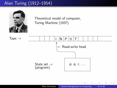
Theoretical model of computer,Turing Machine (1937)
Tape → I N P U T
6← Read-write head� �
p, q, r , . . .State set →(program)
Mika Hirvensalo General Background on Computing 42 of 68

Turing Machine
Tape → I N P U T
6← Read-write head� �
p, q, r , . . .State set →(program)
State p:
Reading a, write b (b depends on p and a)
More read-write head (direction depends on p and a)
Move to state q (q depends on p and a)
Transition function δ(p, a) = (q, b,D) (computational step)
Mika Hirvensalo General Background on Computing 43 of 68
Turing Machine
INPUTT−→ OUTPUT
Turing machine has a starting state q0 and final state(s) qf
In the beginning, INPUT is written on the tape, read-writehead set to read the first symbol, and the state is q0
Computation is carried on by applying the transition functionδ again and again until a final state is reached
When qf is reached, the computation stops and the tapecontent is interpreted as OUTPUT
On decision problems, it is enough to have two ending statesqy (yes) and qn (no), and tape content can be ignored
Notation: T (INPUT ) = OUTPUT
Mika Hirvensalo General Background on Computing 44 of 68

Church-Turing Thesis
Church-Turing Thesis:
Turing machine is the exact mathematical counterpart of theintuitive notion of algorithm
Not provable
Not seriously challenged
All known algorithms can be converted into Turing machineformalism
Mika Hirvensalo General Background on Computing 45 of 68

Church-Turing Thesis
Church-Turing Thesis:
Turing machine is the exact mathematical counterpart of theintuitive notion of algorithm
Not provable
Not seriously challenged
All known algorithms can be converted into Turing machineformalism
Mika Hirvensalo General Background on Computing 45 of 68

Church-Turing Thesis
Church-Turing Thesis:
Turing machine is the exact mathematical counterpart of theintuitive notion of algorithm
Not provable
Not seriously challenged
All known algorithms can be converted into Turing machineformalism
Mika Hirvensalo General Background on Computing 45 of 68
Church-Turing Thesis
Church-Turing Thesis:
Turing machine is the exact mathematical counterpart of theintuitive notion of algorithm
Not provable
Not seriously challenged
All known algorithms can be converted into Turing machineformalism
Mika Hirvensalo General Background on Computing 45 of 68
Turing machines
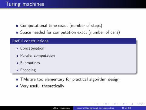
Computational time exact (number of steps)
Space needed for computation exact (number of cells)
Useful constructions
Concatenation
Parallel computation
Subroutines
Encoding
TMs are too elementary for practical algorithm design
Very useful theoretically
Mika Hirvensalo General Background on Computing 46 of 68
Turing machines
Computational time exact (number of steps)
Space needed for computation exact (number of cells)
Useful constructions
Concatenation
Parallel computation
Subroutines
Encoding
TMs are too elementary for practical algorithm design
Very useful theoretically
Mika Hirvensalo General Background on Computing 46 of 68

Programmability
A description of a Turing machine is a finite table oftransitions ⇒ finite string.
The state set describes the program
Part of the input can be interpreted as program
Universal Turing Machine UOn input (T ,w), U simulates the computation of T on input w .
The input w of T must be encoded into the alphabet of UQuite small universal Turing machines exists:
15 states, 2-element alphabet9 states, 3-element alphabet2 states, 18-element alphabet
Mika Hirvensalo General Background on Computing 47 of 68

Programmability
A description of a Turing machine is a finite table oftransitions ⇒ finite string.
The state set describes the program
Part of the input can be interpreted as program
Universal Turing Machine UOn input (T ,w), U simulates the computation of T on input w .
The input w of T must be encoded into the alphabet of U
Quite small universal Turing machines exists:
15 states, 2-element alphabet9 states, 3-element alphabet2 states, 18-element alphabet
Mika Hirvensalo General Background on Computing 47 of 68

Programmability
A description of a Turing machine is a finite table oftransitions ⇒ finite string.
The state set describes the program
Part of the input can be interpreted as program
Universal Turing Machine UOn input (T ,w), U simulates the computation of T on input w .
The input w of T must be encoded into the alphabet of UQuite small universal Turing machines exists:
15 states, 2-element alphabet9 states, 3-element alphabet2 states, 18-element alphabet
Mika Hirvensalo General Background on Computing 47 of 68

Algorithmic undecidability
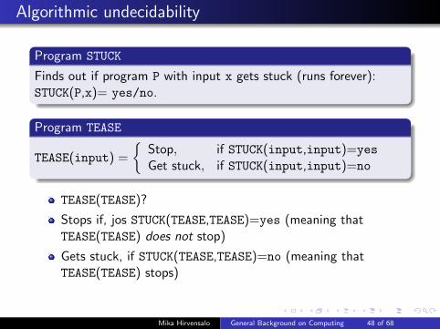
Program STUCK
Finds out if program P with input x gets stuck (runs forever):STUCK(P,x)= yes/no.
Program TEASE
TEASE(input) =
{Stop, if STUCK(input,input)=yes
Get stuck, if STUCK(input,input)=no
TEASE(TEASE)?
Stops if, jos STUCK(TEASE,TEASE)=yes (meaning thatTEASE(TEASE) does not stop)
Gets stuck, if STUCK(TEASE,TEASE)=no (meaning thatTEASE(TEASE) stops) Contradiction! ⇒ no program STUCK
exists
Mika Hirvensalo General Background on Computing 48 of 68

Algorithmic undecidability
Program STUCK
Finds out if program P with input x gets stuck (runs forever):STUCK(P,x)= yes/no.
Program TEASE
TEASE(input) =
{Stop, if STUCK(input,input)=yes
Get stuck, if STUCK(input,input)=no
TEASE(TEASE)?
Stops if, jos STUCK(TEASE,TEASE)=yes (meaning thatTEASE(TEASE) does not stop)
Gets stuck, if STUCK(TEASE,TEASE)=no (meaning thatTEASE(TEASE) stops) Contradiction! ⇒ no program STUCK
exists
Mika Hirvensalo General Background on Computing 48 of 68
Algorithmic undecidability
Program STUCK
Finds out if program P with input x gets stuck (runs forever):STUCK(P,x)= yes/no.
Program TEASE
TEASE(input) =
{Stop, if STUCK(input,input)=yes
Get stuck, if STUCK(input,input)=no
TEASE(TEASE)?
Stops if, jos STUCK(TEASE,TEASE)=yes (meaning thatTEASE(TEASE) does not stop)
Gets stuck, if STUCK(TEASE,TEASE)=no (meaning thatTEASE(TEASE) stops)
Contradiction! ⇒ no program STUCK
exists
Mika Hirvensalo General Background on Computing 48 of 68

Algorithmic undecidability
Program STUCK
Finds out if program P with input x gets stuck (runs forever):STUCK(P,x)= yes/no.
Program TEASE
TEASE(input) =
{Stop, if STUCK(input,input)=yes
Get stuck, if STUCK(input,input)=no
TEASE(TEASE)?
Stops if, jos STUCK(TEASE,TEASE)=yes (meaning thatTEASE(TEASE) does not stop)
Gets stuck, if STUCK(TEASE,TEASE)=no (meaning thatTEASE(TEASE) stops) Contradiction! ⇒ no program STUCK
exists
Mika Hirvensalo General Background on Computing 48 of 68
Algorithmic undecidability
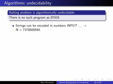
Halting problem is algorithmically undecidable
There is no such program as STUCK
Strings can be encoded in numbers INPUT . . . →N = 7378808584.
Turing Machine operations are interpreted as calculations:N1 = 73 78 808584 → N2 = 72 79 808584
Implies algorithmic undecidability for many mathematicalproblems
Hilbert’s 10th problem
Given an polynomial p(x1, x2, . . . , xn) over integers, does it haveany integer zero? (Undecidable: Yury Matiyasevich 1970)
Matrix problems: Given set {M1, . . . ,Mk} of integer matrices,can we get the zero matrix multiplicatetively?
Mika Hirvensalo General Background on Computing 49 of 68

Algorithmic undecidability
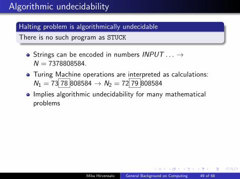
Halting problem is algorithmically undecidable
There is no such program as STUCK
Strings can be encoded in numbers INPUT . . . →N = 7378808584.
Turing Machine operations are interpreted as calculations:N1 = 73 78 808584 → N2 = 72 79 808584
Implies algorithmic undecidability for many mathematicalproblems
Hilbert’s 10th problem
Given an polynomial p(x1, x2, . . . , xn) over integers, does it haveany integer zero? (Undecidable: Yury Matiyasevich 1970)
Matrix problems: Given set {M1, . . . ,Mk} of integer matrices,can we get the zero matrix multiplicatetively?
Mika Hirvensalo General Background on Computing 49 of 68
Algorithmic undecidability
Halting problem is algorithmically undecidable
There is no such program as STUCK
Strings can be encoded in numbers INPUT . . . →N = 7378808584.
Turing Machine operations are interpreted as calculations:N1 = 73 78 808584 → N2 = 72 79 808584
Implies algorithmic undecidability for many mathematicalproblems
Hilbert’s 10th problem
Given an polynomial p(x1, x2, . . . , xn) over integers, does it haveany integer zero? (Undecidable: Yury Matiyasevich 1970)
Matrix problems: Given set {M1, . . . ,Mk} of integer matrices,can we get the zero matrix multiplicatetively?
Mika Hirvensalo General Background on Computing 49 of 68

Measuring time/space
Gluing alphabet symbols together results in a bigger alphabetand more δ-rules, but smaller computations time (constantimprovement)
“Increasing hardware makes computation faster”(constant improvement)
Time / Space -resources should be measured only up tomultiplicative constant.
Mika Hirvensalo General Background on Computing 50 of 68

Ordo-notation
Measuring computational resources
Computational resources (time/space) should be measuredignoring the multiplicative constants
Example
Algorithms A1, A2, A3, and A4 consume respectively 2n6, 600n3,40000n, and 2n
1010 steps to accomplish their tasks. Ignoring themultiplicative constants, their running times are around n6, n3, n,and 2n. Hence A3 is the fastest and A4 the slowest.
Mika Hirvensalo General Background on Computing 51 of 68

Ordo-notation
Definition
f (x) = O(g(x)), if there are constants K > 0 and M > 0 so that
|f (x)| ≤ K |g(x)| ,
whenever x ≥ M.
Example
x5 − 20x4 − 9x3 − 6x2 − 12x − 4 = O(x5)
Example
xn = O(mx)
for each n ∈ N and m > 1.
Mika Hirvensalo General Background on Computing 52 of 68

Ordo-notation
Definition
f (x) = O(g(x)), if there are constants K > 0 and M > 0 so that
|f (x)| ≤ K |g(x)| ,
whenever x ≥ M.
Example
x5 − 20x4 − 9x3 − 6x2 − 12x − 4 = O(x5)
Example
xn = O(mx)
for each n ∈ N and m > 1.
Mika Hirvensalo General Background on Computing 52 of 68

Ordo-notation
Definition
f (x) = O(g(x)), if there are constants K > 0 and M > 0 so that
|f (x)| ≤ K |g(x)| ,
whenever x ≥ M.
Example
x5 − 20x4 − 9x3 − 6x2 − 12x − 4 = O(x5)
Example
xn = O(mx)
for each n ∈ N and m > 1.
Mika Hirvensalo General Background on Computing 52 of 68

Ordo-notation
Definition
f (x) = O(g(x)), if there are constants K > 0 and M > 0 so that
|f (x)| ≤ K |g(x)| ,
whenever x ≥ M.
Example
x5 − 20x4 − 9x3 − 6x2 − 12x − 4 = O(x5)
Example
xn = O(mx)
for each n ∈ N and m > 1.
Mika Hirvensalo General Background on Computing 52 of 68

Notations
Definition
A finite set Σ = {a1, . . . , an} is called an alphabet. The set of allstrings (words) over alphabet Σ is denoted by Σ∗. A formallanguage over alphabet Σ is a subset of Σ∗.
Example
Any Turing machine T defines a formal languageL(T ) = {w ∈ Σ∗ | The computation of T on input w stops}
Definition
A formal language L ⊆ Σ∗ is recursively enumerable if it can beaccepted by a Turing machine, meaning that w ∈ L ⇐⇒ T haltson input w . The set of recursively enumerable languages isdenoted by RE.
Mika Hirvensalo General Background on Computing 53 of 68

Notations
Definition
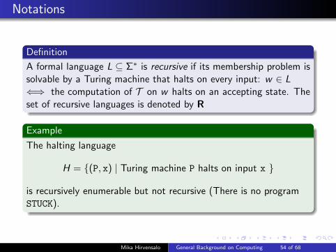
A formal language L ⊆ Σ∗ is recursive if its membership problem issolvable by a Turing machine that halts on every input: w ∈ L⇐⇒ the computation of T on w halts on an accepting state. Theset of recursive languages is denoted by R
Example
The halting language
H = {(P, x) | Turing machine P halts on input x }
is recursively enumerable but not recursive (There is no programSTUCK).
Mika Hirvensalo General Background on Computing 54 of 68

Notations
Definition
A formal language L ⊆ Σ∗ is recursive if its membership problem issolvable by a Turing machine that halts on every input: w ∈ L⇐⇒ the computation of T on w halts on an accepting state. Theset of recursive languages is denoted by R
Example
The halting language
H = {(P, x) | Turing machine P halts on input x }
is recursively enumerable but not recursive (There is no programSTUCK).
Mika Hirvensalo General Background on Computing 54 of 68

Polynomial Time Computation
Straightforward to design: On input w = a1 . . . an (denoten = |w |), machine counts nk steps and then stops.
Can run in parallel with any other TM
Polynomial Time Turing Machines
On any input w , the machine stops in at most nk steps.
The decision (yes/no) depends on the halting state:
If machine stops because the “time” is up, the answer is “no”(reject)If machine finishes its computation in time bound, the answercan be yes (accept) or (no) depending on the input
k is a parameter that can be chosen freely
Mika Hirvensalo General Background on Computing 55 of 68
Polynomial Time Computation
Example
Product is solvable in O(n2) steps (normal multiplication)
Example
Primality is solvable in O(n6+ε) steps (highly nontrivial)
Definition
P is the set of formal languages accepted by polynomial-timeTuring Machines (Practical computation with no errors)
Mika Hirvensalo General Background on Computing 56 of 68

Turing Machine generalizations
Nondeterministic
Instead of single transition δ(p, a) = (q, b,D) the machine canchoose its action from a finite set (p, a) −→ (qi , bi ,Di ) (transitionrelation).
A nondeterministic Turing machine does not define a function
but a relation INPUTT−→ OUTPUT
Probabilistic
Same as nondeterministic, but all transitions occur with a givenprobability (p, a)
pi−→ (qi , bi ,Di )
A probabilistic Turing machine does not define a function buta probability distribution over OUTPUT s, depending on theINPUT .
Mika Hirvensalo General Background on Computing 57 of 68

Turing Machine generalizations
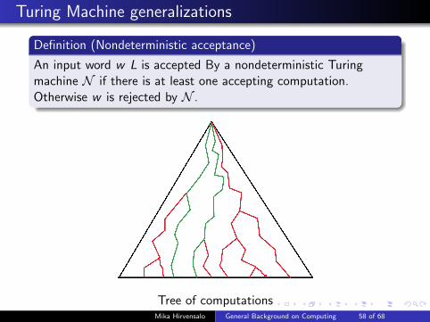
Definition (Nondeterministic acceptance)
An input word w L is accepted By a nondeterministic Turingmachine N if there is at least one accepting computation.Otherwise w is rejected by N .
Tree of computations
Mika Hirvensalo General Background on Computing 58 of 68

Turing Machine generalizations
Definition (Nondeterministic acceptance)
An input word w L is accepted By a nondeterministic Turingmachine N if there is at least one accepting computation.Otherwise w is rejected by N .
Tree of computations
Mika Hirvensalo General Background on Computing 58 of 68
Turing Machine generalizations
Definition (Nondeterministic acceptance)
An input word w L is accepted By a nondeterministic Turingmachine N if there is at least one accepting computation.Otherwise w is rejected by N .
Tree of computationsMika Hirvensalo General Background on Computing 58 of 68
Turing Machine generalizations
Definition (Monte Carlo Model)
An input word w is accepted by a probabilistic Turing Machine P,if the acceptance probability for w is at least 2
3 A word is rejectedis its acceptance probability is at most 1
3 .
Definition (Las Vegas Model)
An input word w is accepted by a probabilistic Turing machine, ifits acceptance probability is 1. A word is rejected, if it acceptanceprobability is at most 1
2 .
Mika Hirvensalo General Background on Computing 59 of 68

Turing Machine generalizations
Example (Nondeterministic Factorization Algorithm)
1 Input m = n1 . . .mn in binary
2 For i = 1 to n2 do: guess the i :th digit of a factor f = f1 . . . f n
2
3 Perform division m/f deterministically
4 If f divides m, the run is successful, otherwise not
5 In a succesful case, the algorithm can be re-run on f
For any composide number m, there exists a factor f , andhence there is at least one succesful run of the algorithm.
In general, running a nondeterministic algorithm correspondsto guessing and verification
Mika Hirvensalo General Background on Computing 60 of 68

Important complexity classes
Definition
P is the class of languages that can be accepted bypolynomial time determinstic Turing machines
NP is the class of languages that can be accepted bynondeterministic polynomial time Turing machines
BPP is the class of languages that can be accepted byprobabilistic polynomial time Turing machines with MonteCarlo acceptance model (practical computability)
Clearly P ⊆ NP and P ⊆ BPP.
Mika Hirvensalo General Background on Computing 61 of 68

P vs. NP
For any nondeteministic Turing machine machine, the numberof computational choices can be assumed two
Machine “tosses coin” on each step
Guiding string: s = s1s2 . . . snk ; si tells which nondeterministicoption to take (outcomes of the “coin tosses”)
Computing with a guiding string is deterministic: a guidingstring determines a path in the tree of computations
w ∈ L ⇔ if there is a guiding string s leading to an acceptingfinal state. Hence:
Nondeterministic computing= guessing the guiding string + computing deterministically
Mika Hirvensalo General Background on Computing 62 of 68

P vs. NP
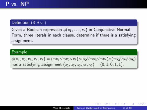
Definition (3-Sat)
Given a Boolean expression φ(x1, . . . , xn) in Conjunctive NormalForm, three literals in each clause, determine if there is a satisfyingassignment.
Example
φ(x1, x2, x3, x4, x5) = (¬x1∨¬x2∨x3)∧(x2∨¬x3∨¬x4)∧(¬x3∨x4∨x5)has a satisfying assignment (x1, x2, x3, x4, x5) = (0, 1, 0, 1, 1).
Nondeterministic algorithm for 3-Sat
1 For i = 1 to n do: Guess value vi for xi2 Check whether φ(v1, . . . , vn) has truth value 1.
Mika Hirvensalo General Background on Computing 63 of 68

P vs. NP
Definition (3-Sat)
Given a Boolean expression φ(x1, . . . , xn) in Conjunctive NormalForm, three literals in each clause, determine if there is a satisfyingassignment.
Example
φ(x1, x2, x3, x4, x5) = (¬x1∨¬x2∨x3)∧(x2∨¬x3∨¬x4)∧(¬x3∨x4∨x5)has a satisfying assignment (x1, x2, x3, x4, x5) = (0, 1, 0, 1, 1).
Nondeterministic algorithm for 3-Sat
1 For i = 1 to n do: Guess value vi for xi2 Check whether φ(v1, . . . , vn) has truth value 1.
Mika Hirvensalo General Background on Computing 63 of 68

P vs. NP
Deterministic algorithm for 3-Sat
1 Go through all values v1 . . . vn ∈ {0, 1}n;
2 For each valuation, check whether φ(v1, . . . , vn) has truthvalue 1
The deterministic version requires 2n rounds, whereas thenondeterministic version has only one round.
Can you do better (deterministically)?
Uwe Schoning:O(( 4
3 )n) algorithm
Mika Hirvensalo General Background on Computing 64 of 68
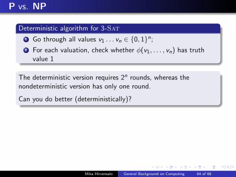

P vs. NP
Can you solve 3-Sat deterministically in nk time?
No-one knows
3-Sat is NP-complete
All other NP problems reduce to it
P algorithm to 3-Sat will give a P algorithm for all NPproblems
A polynomial algorithm for 3-Sat would imply that “guessing” isequally difficult to “verifying”; NP would be equal to P.
Mika Hirvensalo General Background on Computing 65 of 68
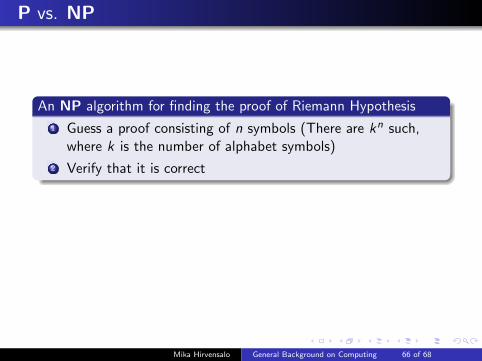
P vs. NP
An NP algorithm for finding the proof of Riemann Hypothesis
1 Guess a proof consisting of n symbols (There are kn such,where k is the number of alphabet symbols)
2 Verify that it is correct
If P = NP there is also a deterministic polynomial-time algorithmfor the same task
Probably P 6= NP, but how to prove it?
Mika Hirvensalo General Background on Computing 66 of 68
P vs. NP
Clay Mathematics Institute:
The solver of the P vs. NP problem will get
Mika Hirvensalo General Background on Computing 67 of 68

P vs. NP
Clay Mathematics Institute:
The solver of the P vs. NP problem will get
Mika Hirvensalo General Background on Computing 67 of 68
Further complexity classes
Complexity Zoo athttps://complexityzoo.uwaterloo.ca/Complexity Zoo
496 complexity classes by now
Mika Hirvensalo General Background on Computing 68 of 68
Further complexity classes
Complexity Zoo athttps://complexityzoo.uwaterloo.ca/Complexity Zoo
496 complexity classes by now
Mika Hirvensalo General Background on Computing 68 of 68