further maths notes - physicsservellophysicsservello.com.au/files/further+summary.pdf · further...

Further Maths Notes

Common Mistakes

• Read the bold words in the exam!

• Always check data entry

• Remember to interpret data with the multipliers specified (e.g. in thousands)

• Write equations in terms of variables

• Watch for a+bx and ax+b forms

• Remember to seasonalise data after predictions • Ensure calculator is in degrees • Always write true bearings as 90°T • Always check the feasible region with a point • Never delete an answer • Least squares gradient has Sy on top • When crashing, look for vertices common to multiple

paths

2007

Further Mathematics Units 3 and 4 Revision 2

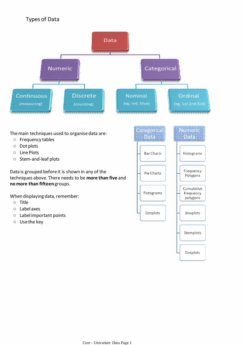
Frequency tables○

Dot plots○

Line Plots○

Stem-and-leaf plots○

The main techniques used to organise data are:

Data is grouped before it is shown in any of the techniques above. There needs to be more than five and no more than fifteen groups.

Title○

Label axes○

Label important points○

Use the key○

When displaying data, remember:

Types of Data

Core - Univariate Data Page 1

Skew determines where data is most spread out. Most distributions are skewed.Skewed data is usually a result of a barrier preventing data from going past a limit.

Negatively skewed data has a 'tail' pointing to the left.

Most of the data is concentrated around the higher values of x○

Mean, median and mode will not be the same○

Mean, median and mode are located in the body of the curve (the right)○

This means that:

Positively skewed data has a 'tail' pointing to the right.

Most of the data is concentrated around the lower values of x○

Mean, median and mode will not be the same○

Mean, median and mode are located in the body of the curve (the left)○

This means that:

For skewed data, the median and IQR is usually used.

Perfectly symmetrical data has an equal mean, median and mode.Frequency histograms and polygons show a bell-shaped curve.

Bimodal data shows two equal modes. This usually indicates that there are two groups of data that need to be separated (eg. height of boys and girls)

Skew


The following summary statistics are usually used together:

Mean and standard deviation○

Median and IQR○

Mode and range○

ModeThe mode is the most commonly occurring value. There can be two or more modes.

The mode is not usually an accurate measure of centre, and is only used when there is a high number of scores.

MedianThe median is the middle value. 50% of data lies either side of the median.

If there are two middle values, it is their average. To calculate the median of grouped data, use a cumulative frequency table.

The median does not take all values into account, and is therefore not affected by extreme values. The median is usually used for skewed distributions. It may not be equal to one of the values in the data set.

MeanThe mean is the average value.

For ungrouped data:

For grouped data:

The mean is not necessarily equal to a value in the data set.The mean takes all data into account, and is therefore affected by extreme values.

RangeThe range is the difference between the smallest value and the largest. It is influenced by outliers.For grouped data, the range is the difference between the highest and

lowest groups with values.

Interquartile rangeThe IQR is the range between which 50% of values lie. It is not affected

by outliers. It is best obtained using a calculator.

Statistic Term number

Q1

Median

Q3

Analysing data


The variance is the square of the standard deviation. Both values show the distribution of data around the mean.

•

Both standard deviation and variance are always positive numbers.•Both standard deviation and variance are affected by outliers.•To estimate the standard deviation of a dataset, the following formula is used:•

This formula accounts for 95% of data being within two standard deviations of the mean.

The 68-95-99.7 Rule

68% of values lie within one standard deviation of the mean.95% of values lie within two standard deviations of the mean.

99.7% of values lie within three standard deviations of the mean.

Z-ScoresZ-scores are used to compare values between different sets of data. For example, the height of a girl can be compared with the height of a boy by comparing them with their gender and age.

The formula for z-scores is:

The following formulas can also be used to determine information:

The z-scores then function like normal data distributions with a mean of zero and a standard deviation of one. The 68-95-99.7 rule can then be applied to the standardised data.

Standard Deviation and Variance


Categorical - Categorical○

Numeric - Categorical○

Numeric - Numeric○

Bivariate data sets can be of three types:

For any bivariate data set, one variable is dependent and the other independent.

The dependent variable responds to change in the independent variable.The independent variable explains the change in the dependent variable.

r values - perfect, strong, moderate, weak or none

r² values

Strength○

Linear or non-linear

Form○

Positive or negative

Direction○

The objective of bivariate analysis is to determine whether a relationship exists and if so, its:

y

xIndependent

variable

Dependent variable

The dependent variable is always plotted on the y-axis, and the independent on the x-axis.

Types of Bivariate Data

Core - Bivariate Data Page 5

This diagram shows values of Pearson's Product-Moment Correlation Coefficient and what strength relationship they represent.

Positive values always represent relationships with a positive gradient, and negative values always represent relationships with a negative gradient.

The Coefficient of Determination is equal to r². It describes the influence the independent variable has on the dependent variable. It is usually expressed as a percentage. The standard analysis is:

The coefficient of determination calculated to be [r²] shows that [r²%] of the variation in [dependent variable] can be explained by variation in [independent variable]. The other [(100-r²)]%

of variation in [dependent variable] can be explained by other factors or influences.

It is designed for linear data only○

It should be used with caution if outliers are present○

Note that:

Correlation


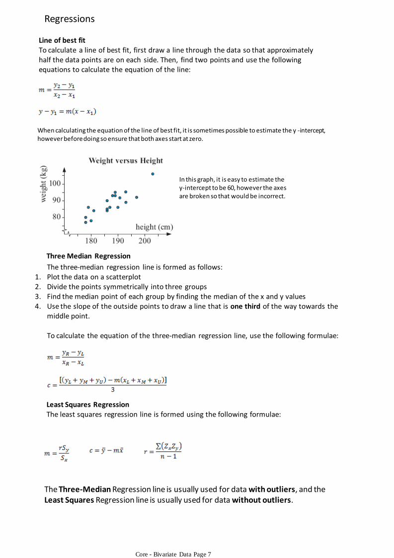
Line of best fitTo calculate a line of best fit, first draw a line through the data so that approximately half the data points are on each side. Then, find two points and use the following equations to calculate the equation of the line:

When calculating the equation of the line of best fit, it is sometimes possible to estimate the y -intercept, however before doing so ensure that both axes start at zero.

In this graph, it is easy to estimate the y-intercept to be 60, however the axes are broken so that would be incorrect.

Three Median Regression

The three-median regression line is formed as follows:Plot the data on a scatterplot1.Divide the points symmetrically into three groups2.Find the median point of each group by finding the median of the x and y values3.Use the slope of the outside points to draw a line that is one third of the way towards the middle point.

4.

To calculate the equation of the three-median regression line, use the following formulae:

Least Squares RegressionThe least squares regression line is formed using the following formulae:

The Three-Median Regression line is usually used for data with outliers, and the Least Squares Regression line is usually used for data without outliers.

Regressions


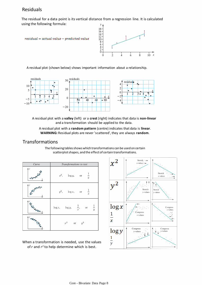
The residual for a data point is its vertical distance from a regression line. It is calculated using the following formula:

A residual plot (shown below) shows important information about a relationship.

A residual plot with a valley (left) or a crest (right) indicates that data is non-linearand a transformation should be applied to the data.

A residual plot with a random pattern (centre) indicates that data is linear.WARNING: Residual plots are never 'scattered', they are always random.

TransformationsThe following tables shows which transformations can be used on certain

scatterplot shapes, and the effect of certain transformations.

When a transformation is needed, use the values of r and r² to help determine which is best.

Residuals


Time series data is simply data with a timeframe as the independent variable.There are four ways in which it can be described:

Secular Trend1.Data displays a trend (or secular trend) when a consistent increase or decrease can be seen in the data over a significant period of time. A trend line can be fitted to such data.

Seasonality2.Seasonal data changes or fluctuates at given intervals, with given intensities. For example, sales of warm drinks might fluctuate in winter. This data can be deseasonalised.

Cyclic3.Cyclic data shows fluctuations, but not at consistent intervals, amplitudes or seasons. This includes data such as stock prices.

Random4.Random data shows no pattern. All fluctuations occur by chance and cannot be predicted.

Summarising Time Series Data


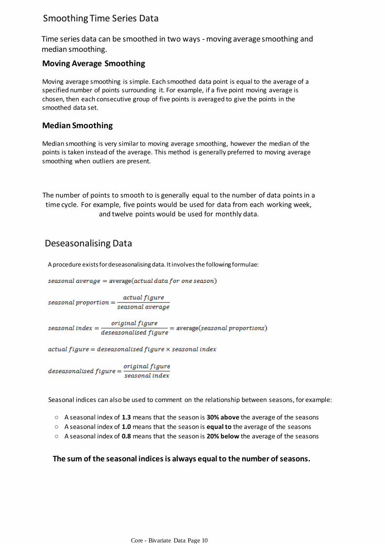
Time series data can be smoothed in two ways - moving average smoothing and median smoothing.

Moving Average Smoothing

Moving average smoothing is simple. Each smoothed data point is equal to the average of a specified number of points surrounding it. For example, if a five point moving average is

chosen, then each consecutive group of five points is averaged to give the points in the smoothed data set.

Median Smoothing

Median smoothing is very similar to moving average smoothing, however the median of the points is taken instead of the average. This method is generally preferred to moving average

smoothing when outliers are present.

The number of points to smooth to is generally equal to the number of data points in a time cycle. For example, five points would be used for data from each working week,

and twelve points would be used for monthly data.

Deseasonalising Data

A procedure exists for deseasonalising data. It involves the following formulae:

Seasonal indices can also be used to comment on the relationship between seasons, for example:

A seasonal index of 1.3 means that the season is 30% above the average of the seasons○

A seasonal index of 1.0 means that the season is equal to the average of the seasons○

A seasonal index of 0.8 means that the season is 20% below the average of the seasons○

The sum of the seasonal indices is always equal to the number of seasons.

Smoothing Time Series Data


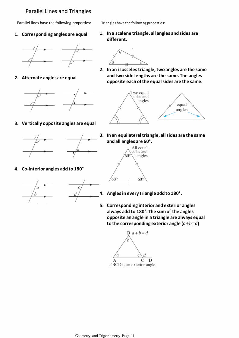
Parallel lines have the following properties:

Corresponding angles are equal1.

Alternate angles are equal2.

Vertically opposite angles are equal3.

Co-interior angles add to 180°4.

Triangles have the following properties:

In a scalene triangle, all angles and sides are different.

1.

In an isosceles triangle, two angles are the same and two side lengths are the same. The angles opposite each of the equal sides are the same.

2.

In an equilateral triangle, all sides are the same and all angles are 60°.

3.

Angles in every triangle add to 180°.4.

Corresponding interior and exterior angles always add to 180°. The sum of the angles opposite an angle in a triangle are always equal to the corresponding exterior angle (a+b=d)

5.

Parallel Lines and Triangles

Geometry and Trigonometry Page 11

Size of each interiorangle: Size of each exteriorangle:

In a regular polygon, all sides and angles are equal.

The sum of the interior angles of an n-sided polygon is:

The sum of the exterior angles of any polygon is:

s=360°

Right Angled Triangles

The Pythagorean Theorem states that:

Note that c always refers to the hypotenuse, however exams may refer to the sides differently.

Regular Polygons


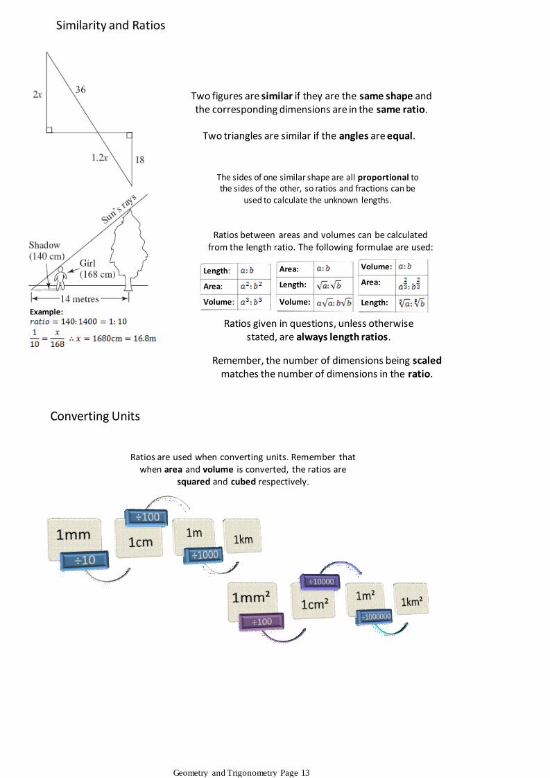
Two figures are similar if they are the same shape and the corresponding dimensions are in the same ratio.

Two triangles are similar if the angles are equal.

The sides of one similar shape are all proportional to the sides of the other, so ratios and fractions can be

used to calculate the unknown lengths.

Example:

Converting Units

Ratios between areas and volumes can be calculated from the length ratio. The following formulae are used:

Length:

Area:

Volume:

Ratios are used when converting units. Remember that when area and volume is converted, the ratios are

squared and cubed respectively.

Area:

Length:

Volume:

Volume:

Area:

Length:

Ratios given in questions, unless otherwise stated, are always length ratios.

Remember, the number of dimensions being scaledmatches the number of dimensions in the ratio.

Similarity and Ratios


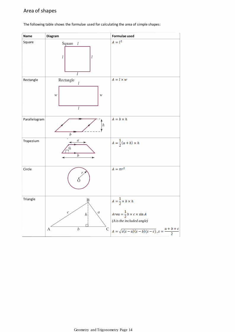
The following table shows the formulae used for calculating the area of simple shapes:

Name Diagram Formulae used

Square

Rectangle

Parallelogram

Trapezium

Circle

Triangle

(A is the included angle)

Area of shapes


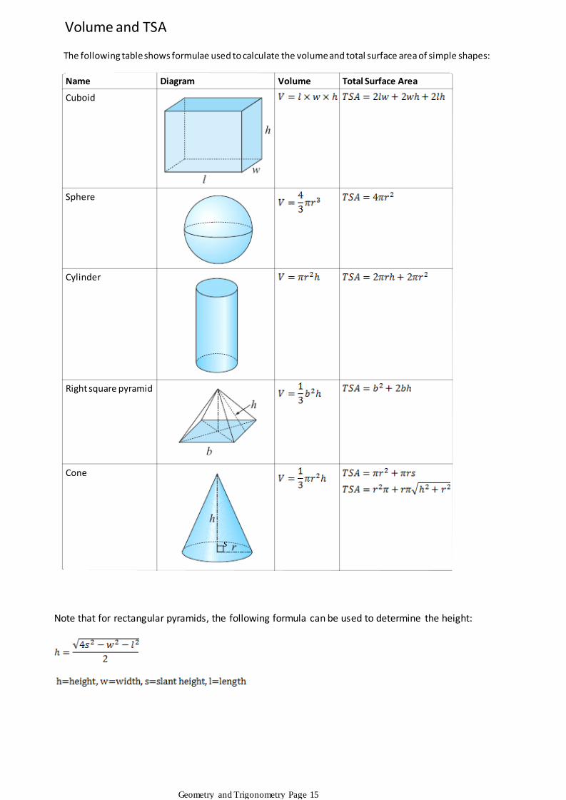
The following table shows formulae used to calculate the volume and total surface area of simple shapes:

Name Diagram Volume Total Surface Area

Cuboid

Sphere

Cylinder

Right square pyramid

Cone

s

Note that for rectangular pyramids, the following formula can be used to determine the height:

Volume and TSA


Right Angled Triangles

The Sine Rule (all triangles)

The sine rule is used with two sides and two corresponding angles.

The Cosine Rule (all triangles)

The cosine rule is used with three sides and one angle.

Trigonometry


A bearing is a way of specifying directionfrom one place to another.

Compass bearings (e.g. S48°W)○

True bearings (e.g. 228°T)○

There are two types of bearings:

Contour maps graphically show heights. Each line on a contour map represents the area on the map where land is exactly that height.

Dense lines show a steep slope, and lines that are spaced apart show a flatter slope.

The slope can be calculated simply by using the rise-over-run formula.

Bearings and Contours


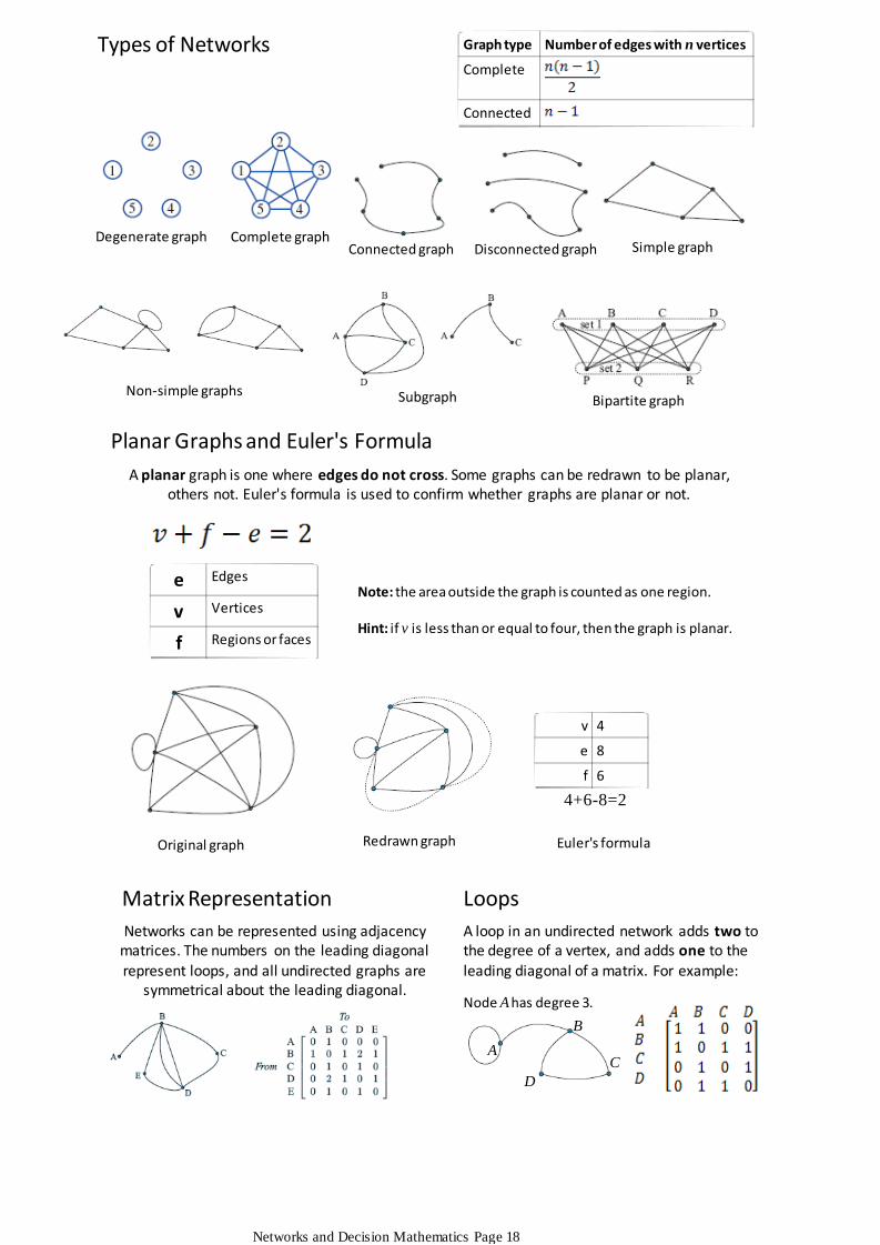
Degenerate graph Complete graphConnected graph Disconnected graph Simple graph

Non-simple graphs Subgraph Bipartite graph

Planar Graphs and Euler's Formula

A planar graph is one where edges do not cross. Some graphs can be redrawn to be planar, others not. Euler's formula is used to confirm whether graphs are planar or not.

e Edges

v Vertices

f Regions or faces

Note: the area outside the graph is counted as one region.

Hint: if v is less than or equal to four, then the graph is planar.

v 4

e 8

f 6

4+6-8=2

Original graph Redrawn graph Euler's formula

Matrix Representation

Networks can be represented using adjacency matrices. The numbers on the leading diagonal represent loops, and all undirected graphs are

symmetrical about the leading diagonal.

Graph type Number of edges with n vertices

Complete

Connected

Loops

A loop in an undirected network adds two to the degree of a vertex, and adds one to the leading diagonal of a matrix. For example:

A

B

C

D

Node A has degree 3.

Types of Networks

Networks and Decision Mathematics Page 18

PathsA path is a sequence of steps between adjacent nodes. In this graph, B-D-A-C

and C-A-B-D are two of the paths which could exist. B-C-D-A could not exist

because B is not adjacent to C.

Eulerian paths and circuitsEulerian paths and circuits pass each edge only once. Eulerian paths exist where there are two or less vertices with odd degree. Eulerian circuits exist when all vertices have even degree. On

the graph above, D-A-C-D-B-A represents an Eulerian path, and no Eulerian circuits exist.

Hamiltonian paths and circuitsHamiltonian paths and circuits are those which pass through each vertex only once. Examples in the above graph include B-A-D-C and D-C-A-B-D.

CircuitsA circuit is a sequence of steps between

adjacent nodes which starts and finishes

at the same vertex. In this graph, B-D-C-A-B and A-D-B-A-D-C-A are two of the circuits

which could exist.

Trees

The nearest neighbour algorithm in which the longest edge, which doesn't disconnect the graph, is removed. This is repeated until no more edges can be removed.

○

Prim's algorithm which involves choosing random vertex as a starting graph and constantly building to it by adding the shortest edges which will connect it to another

node.

○

A tree is a connected, simple graph with no circuits. A spanning tree is a subgraph of a connected graph which contains all the vertices of the original graph. The weight of a spanning

tree is the combined weight of all its edges, and there are two ways in which the minimum-weight spanning tree can be found:

The shortest pathThe shortest path algorithm (or Dijkstra's Algorithm) is used to find the shortest path between two nodes. It involves working from start to finish, labeling each vertex with the shortest path

between it and the starting node.

The Chinese Postman ProblemThe Chinese Postman Problem involves finding the shortest circuit (route) along a network (town) which covers all edges (roads) and starts and finishes at the same spot (the Post Office). It must be

an Eulerian circuit if possible, otherwise the routes between the odd-degree vertices must be travelled twice.

The Travelling Salesman ProblemThe Travelling Salesman Problem (TSP) involves finding the shortest circuit (route) which covers all vertices (houses) in a network (town) in the minimal distance. It must be a Hamiltonian

circuit if possible, but there is no systematic way of solving this problem.

Paths, Circuits and Trees


In a directed graph, each edge has a direction. Also, each vertex in a network can be reachable or unreachable.

In this network, no node is reachable from F, and A is not reachable from B.

Network Flow

Weighted graphs can be used to model the flow of people, water or traffic. The flow is always from the source vertex to the sink vertex. The weight of an edge represents its capacity.

Cuts are used as a way of preventing all flow from source to sink. A valid cut must completely isolate the source from the sink. By adding the weights of the cut edges, the value of a cut can

be obtained. The minimum value cut that can be made represents the maximum flow possible through the network.

If a cut passes through an edge which flows from sink to source, it is called a double cut. The weight of a double cut is equal to the sum of all of its edges which flow from source to sink.

Connectivity MatricesEvery directed network can be represented in a matrix form, like undirected networks. The matrices that represent directed graphs however, are not always symmetrical and can tell us more about a network.

The edges in the network above are represented in the table, which can be translated directly into a matrix. This matrix shows all of the one-stage paths between any two vertices. If this

matrix is squared, the resulting matrix shows the two-step pathways between nodes. The original and the squared matrix can be added to find the winning team in a round-robin

tournament.

Directed Graphs


The network above shows a plan for a project. It could be anything from building a house to getting ready in the morning. The critical path represents the longest path from the start to the

finish, and hence the path on which the finishing time depends. The critical path can be found using forward and backward scanning.

Forward scanning involves finding the earliest start time for every task. Starting at zero, the longest path from the start to each node (the start of each task) is calculated and written in the left-hand box. The number written in the last box is the critical time.

Backward scanning involves finding the longest path from the finish vertex to each node (the start of each task). This gives us the latest start time for each activity, before it delays the finishing time of the project. The slack (or float) time, in which nothing is being done on a particular path, is calculated by LST - EST. The critical path can be found by looking for activities with a float time of zero.

Crashing a project

Write down all of the paths from the start node to the finish node, and determine the length of each.

One.

Calculate the cost per day of crashing each activity (note that some questions may already have the cost per day, and watch for reductions that must be made in full)

Two.

Reduce the cheapest (cost per day) activity on the critical path by one day.Three.Calculate the new lengths of all of the paths.Four.Repeat steps three and four, each time using the new longest path after reductions. Five.Stop when the budget is reached or the longest path cannot be reduced. The new critical path is the longest path.

If a project looks like running overtime, it may be crashed. Crashing involves spending extra money to reduce the time taken by certain activities in order to avoid costs of completing the project late. The following steps illustrate the crashing process:

Project Management


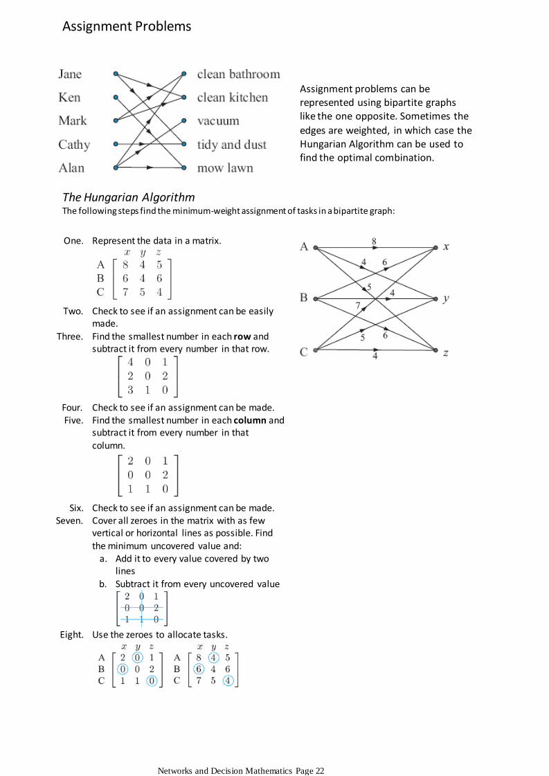
Assignment problems can be represented using bipartite graphs like the one opposite. Sometimes the

edges are weighted, in which case the Hungarian Algorithm can be used to find the optimal combination.

The Hungarian AlgorithmThe following steps find the minimum-weight assignment of tasks in a bipartite graph:

Represent the data in a matrix.One.

Check to see if an assignment can be easily made.

Two.

Find the smallest number in each row and subtract it from every number in that row.

Three.

Check to see if an assignment can be made.Four.Find the smallest number in each column and subtract it from every number in that

column.

Five.

Check to see if an assignment can be made.Six.

Add it to every value covered by two lines

a.

Subtract it from every uncovered valueb.

Cover all zeroes in the matrix with as few vertical or horizontal lines as possible. Find

the minimum uncovered value and:

Seven.

Use the zeroes to allocate tasks.Eight.

Assignment Problems


The following formulae are used to calculate the gradient of a straight line:

The gradient of a straight line is always the coefficient of x. Lines with the same gradient are parallel.

Equation FormEquations can be presented in one of two forms:

Gradient-intercept form: y=ax+b

General form: ax+by=c

Linear Basics

Graphs and Relations Page 23

Simultaneous EquationsExample:At the footy, three pies and five buckets of chips costs $16.50.Also, 4 pies and 3 buckets of chips costs $15.40.

3p+5c=16.54p+3c=15.6

What is the cost of pies and chips?Using a calculator, pies cost $2.50 and chips $1.80.

Break-Even Analysis

The break-even point is where cost equals revenue. On the graph opposite, this is represented as x1.

Profit and loss is defined by the difference between this value and the actual number of products sold.

Line segment graphs occur when more than one equation exists for a graph. For example, cyclists

might ride at different speeds for different stages of a journey. Their distance from a given point

would be represented by a line segment graph.

Step Graphs

Line Segment Graphs

Step graphs represent relationships defined by a series of zero-gradient equations, in situations like

parking costs and postage costs.

Non-linear Graphs

The maximum point○

The minimum point○

Large and small rates of change○

Questions may ask for interpretations of non-linear graphs. Key knowledge includes:

Applications


This is the general form for an exponential graph. It can be obtained from a set of data by using the

power regression on the calculator.

The following graphs show the shape of relationships with different values of n.

Value of n Graph

-2

-1

Value of n Graph

1

2

3

NEGATIVE POSITIVE

Exponential Graphs


An inequality differs from an equation because it defines a region of a graph, as opposed to a line.

If an inequality is in either general form or gradient-intercept form then the '<' sign will refer to the region below the boundary and the '>' sign will refer to the

region above the boundary.

Always remember to use a key and dot the line if it is not included.

Inequalities


Inequalities can be used to model situations. To model a situation, a number of constraints are used. Sometimes information can be represented in a table.

Example:Fred can buy sausages and hamburgers for a BBQ dinner. He cannot buy more than twelve items.Let x be sausages and y be hamburgers.

Sausages cost $2 each and hamburgers $1. He cannot spend more than $15.

Change each inequality to an equation by replacing the inequality with an equals sign.

a.

Plot the lines, dotting those where the line itself is not included,b.Shade the feasible region and write a key.c.Check that a point within the feasible region fits all the inequalities.d.

To graph a set of inequalities:

Problem Solving

Find the values of the extreme points by getting the intercepts between the lines. Make sure each of the extreme points chosen is inside the feasible region.

One.

Write the x and y values of these intercepts in a table.Two.Make a new column in the table and write the result of the objective function for the x and y values in that row.

Three.

Look for the lowest or highest (depending on the question) value for the objective function. If there a two lowest or highest values, the ideal values of x and y are not only those listed, but also every value on the line joining those points.

Four.

To solve a linear programming problem, an objective function is required. This objective function calculates the cost given the values of x and y. The following steps show how to use the values if the extreme points to solve a linear programming problem:

The Sliding Ruler Method

Give the objective function an equal value to change it into an equation.One.Plot it on a graph of the feasible region.Two.Slide a clear ruler along the page, keeping the same gradient, until the last point in the feasible region is reached. The direction to slide the ruler depends on whether

the objective function is being minimised or maximised.

Three.

The last point that is reached in the feasible region is equal to the ideal x and yvalues for the problem.

Four.

If the ruler finishes on a line, all the points on that line are ideal values.

The Sliding Ruler method is an alternative to the method above. Its procedure is:

Modeling Inequalities


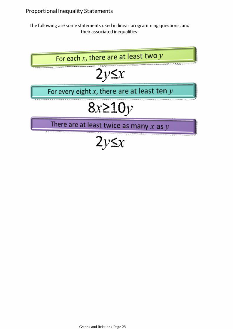
The following are some statements used in linear programming questions, and their associated inequalities:

Proportional Inequality Statements


further maths notes - physicsservellophysicsservello.com.au/files/further+summary.pdf · further...

Documents