VCE Further MathsVCE Further MathsLeast Square Regression using the calculator

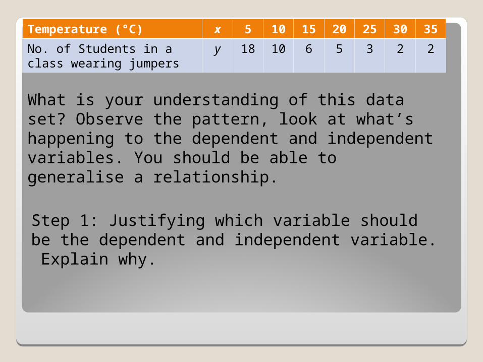
Temperature (°C) x 5 10 15 20 25 30 35

No. of Students in a class wearing jumpers

y 18 10 6 5 3 2 2

What is your understanding of this data set? Observe the pattern, look at what’s happening to the dependent and independent variables. You should be able to generalise a relationship.

Step 1: Justifying which variable should be the dependent and independent variable. Explain why.

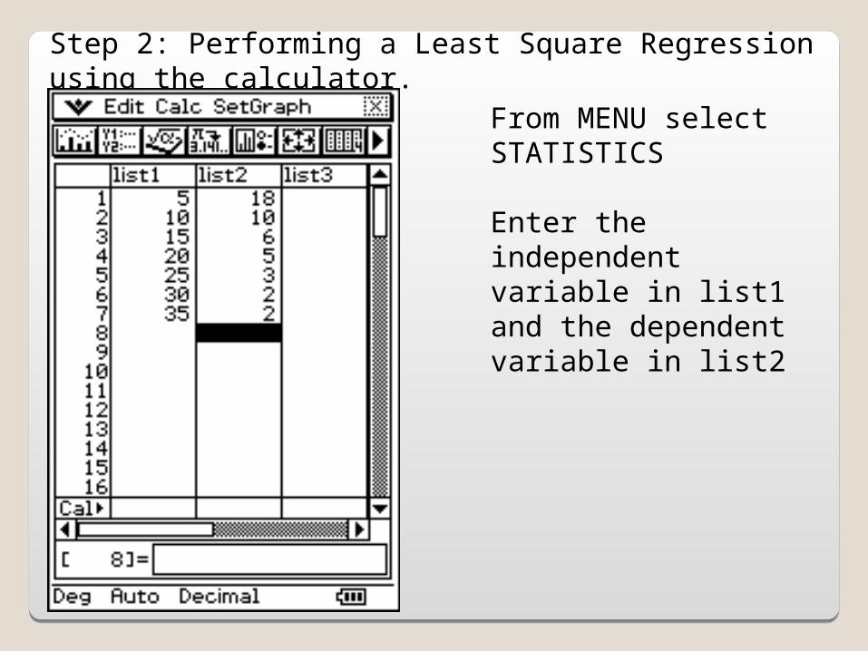
Step 2: Performing a Least Square Regression using the calculator.

From MENU select STATISTICS

Enter the independent variable in list1and the dependent variable in list2

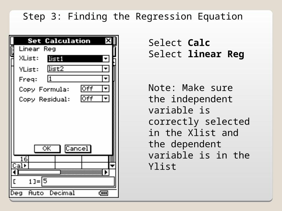
Step 3: Finding the Regression Equation

Select Calc Select linear Reg

Note: Make sure the independent variable is correctly selected in the Xlist and the dependent variable is in the Ylist

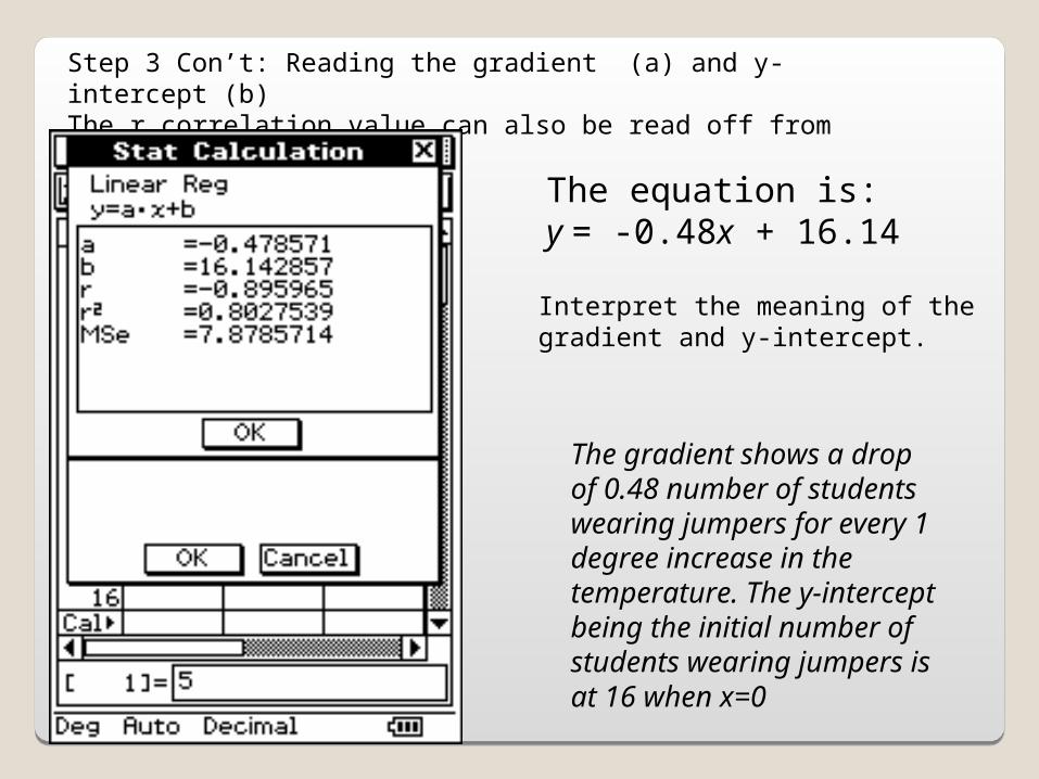
Step 3 Con’t: Reading the gradient (a) and y-intercept (b)The r correlation value can also be read off from this screen

The equation is:y = -0.48x + 16.14

Interpret the meaning of the gradient and y-intercept.

The gradient shows a drop of 0.48 number of students wearing jumpers for every 1 degree increase in the temperature. The y-intercept being the initial number of students wearing jumpers is at 16 when x=0

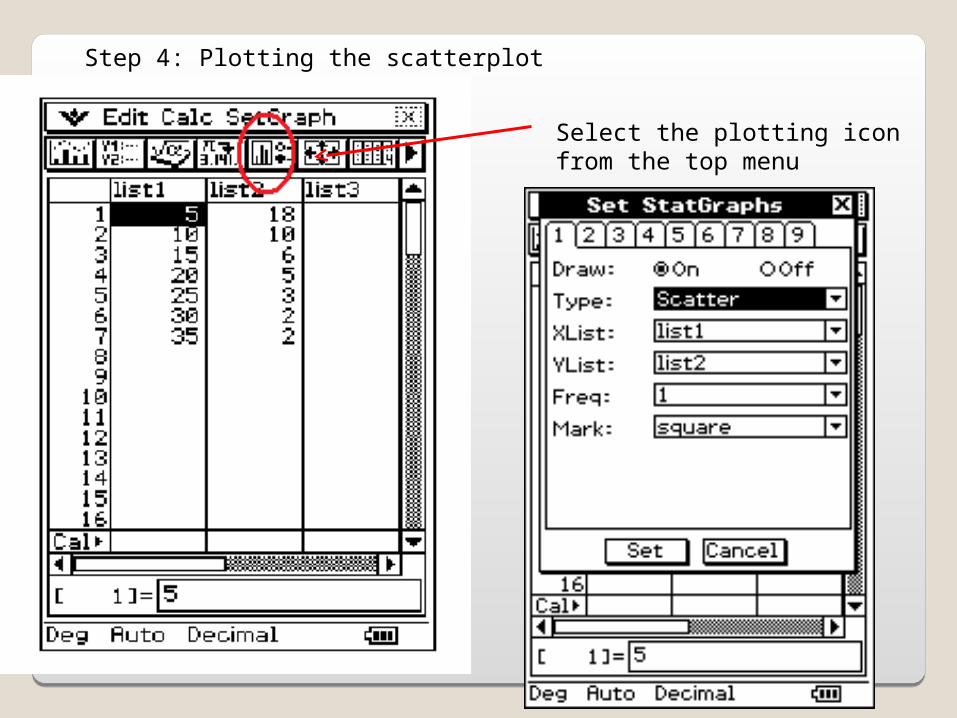
Step 4: Plotting the scatterplot

Select the plotting icon from the top menu

Select the graphing icon from the top menu

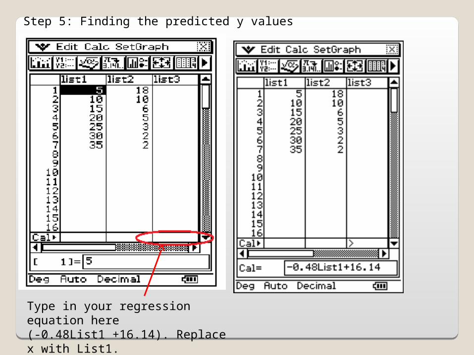
Step 5: Finding the predicted y values

Type in your regression equation here(-0.48List1 +16.14). Replace x with List1.

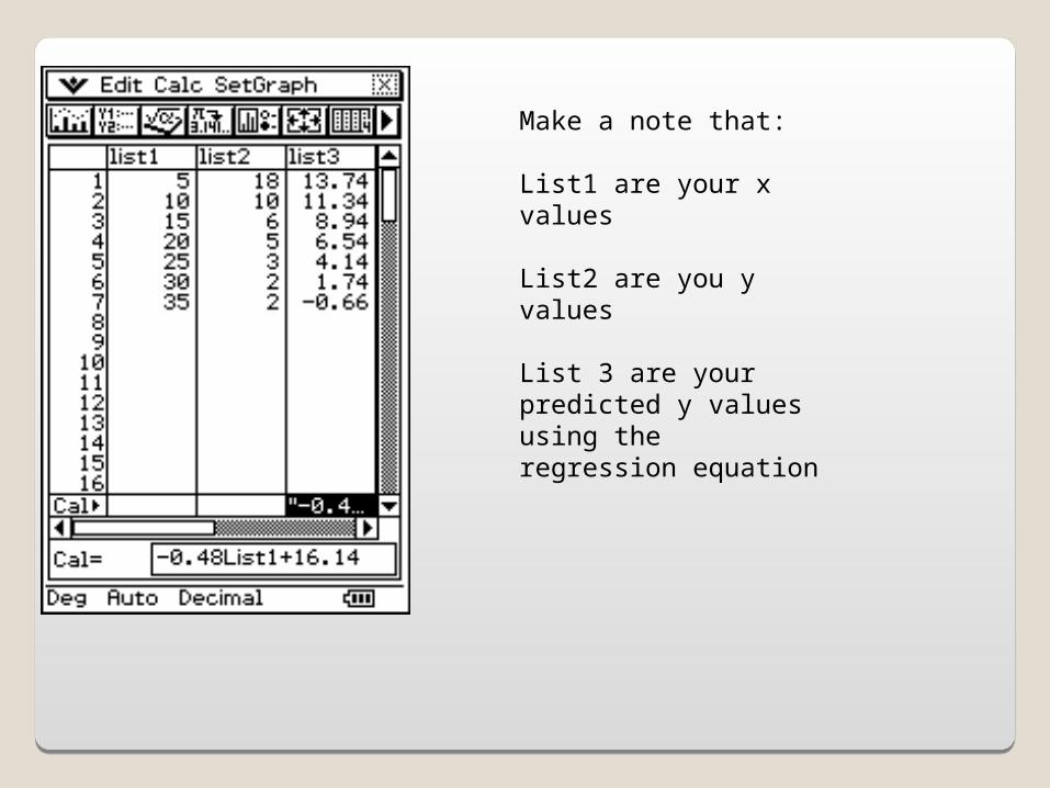
Make a note that:

List1 are your x values

List2 are you y values

List 3 are your predicted y values using the regression equation

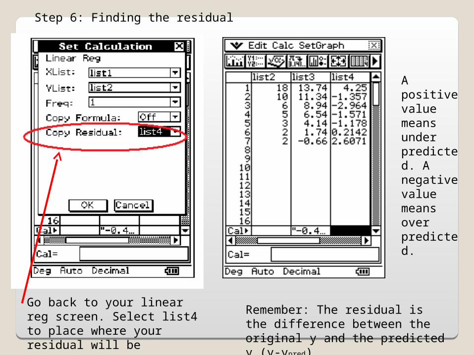
Step 6: Finding the residual

Go back to your linear reg screen. Select list4 to place where your residual will be

Remember: The residual is the difference between the original y and the predicted y (y-ypred)

A positive value means under predicted. A negative value means over predicted.

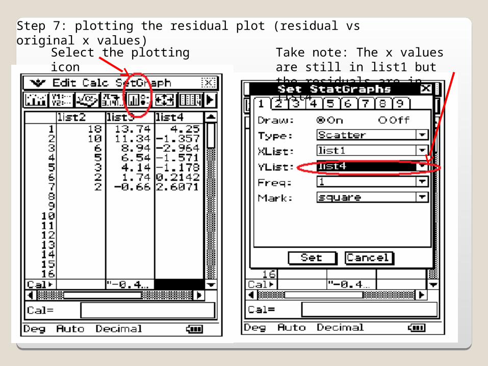
Step 7: plotting the residual plot (residual vs original x values)

Select the plotting icon Take note: The x values are still in list1 but the residuals are in list4

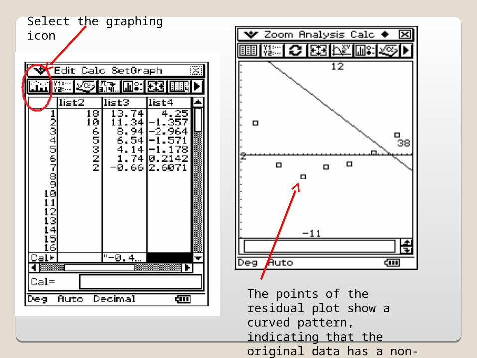
Select the graphing icon

The points of the residual plot show a curved pattern, indicating that the original data has a non-linear relationship

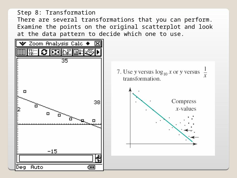
Step 8: TransformationThere are several transformations that you can perform. Examine the points on the original scatterplot and look at the data pattern to decide which one to use.

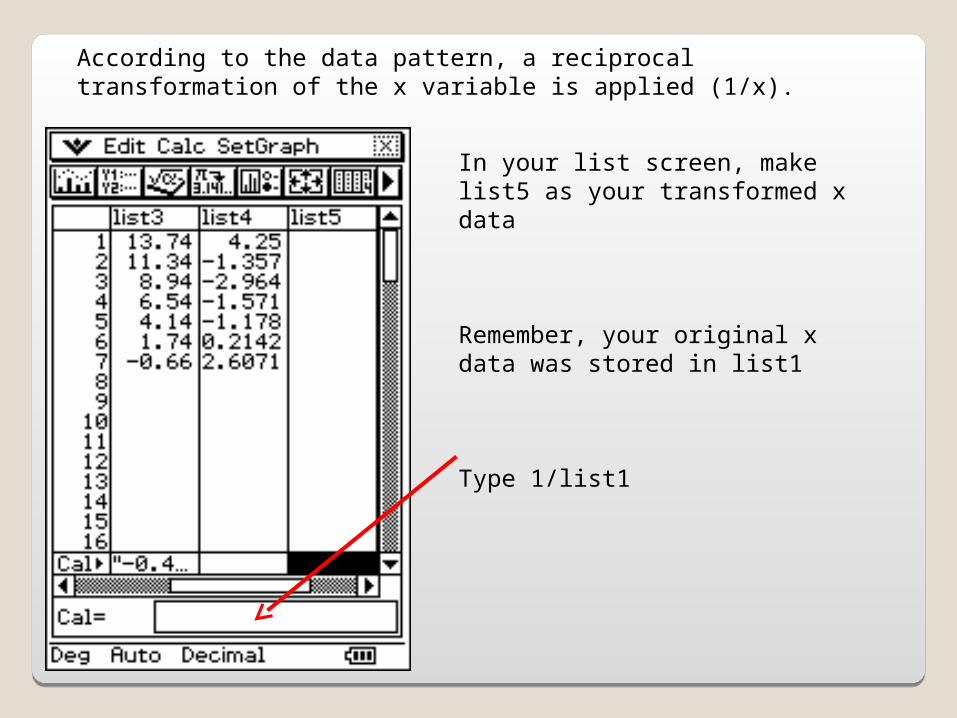
According to the data pattern, a reciprocal transformation of the x variable is applied (1/x).

In your list screen, make list5 as your transformed x data

Remember, your original x data was stored in list1

Type 1/list1

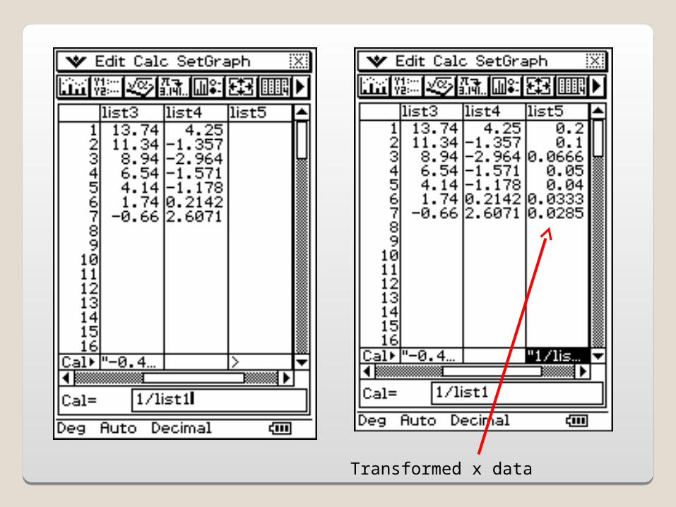
Transformed x data

Step 9: To find your transformed equation

Remember, your new transformed x data are now in list5

Must provide in the order of independent first, then the dependent

We have only transformed the x data therefore, the original y data remains the same in list2

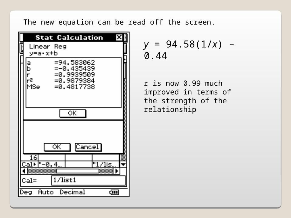
The new equation can be read off the screen.

y = 94.58(1/x) – 0.44

r is now 0.99 much improved in terms of the strength of the relationship

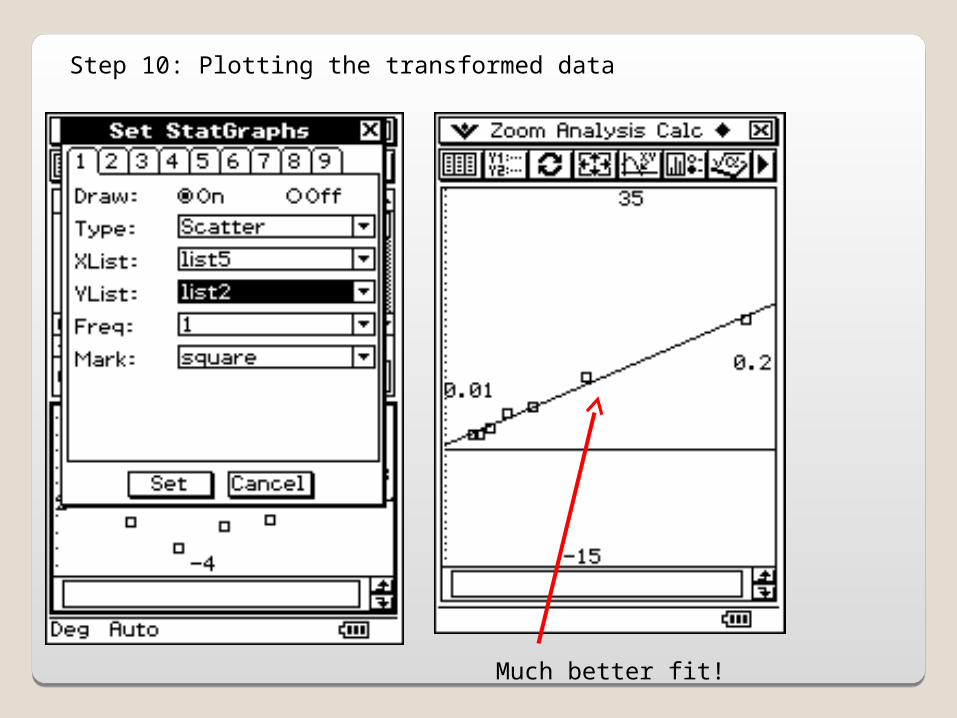
Step 10: Plotting the transformed data

Much better fit!