functional form and structural change qpeople.stern.nyu.edu/wgreene/mathstat/greenechapter6.pdf ·...
TRANSCRIPT

Greene-2140242 book November 19, 2010 1:8
6
FUNCTIONAL FORM ANDSTRUCTURAL CHANGE
Q
6.1 INTRODUCTION
This chapter will complete our analysis of the linear regression model. We begin by ex-amining different aspects of the functional form of the regression model. Many differenttypes of functions are linear by the definition in Section 2.3.1. By using different trans-formations of the dependent and independent variables, binary variables, and differentarrangements of functions of variables, a wide variety of models can be constructed thatare all estimable by linear least squares. Section 6.2 considers using binary variables toaccommodate nonlinearities in the model. Section 6.3 broadens the class of modelsthat are linear in the parameters. By using logarithms, quadratic terms, and interactionterms (products of variables), the regression model can accommodate a wide variety offunctional forms in the data.
Section 6.4 examines the issue of specifying and testing for discrete change in theunderlying process that generates the data, under the heading of structural change. Ina time-series context, this relates to abrupt changes in the economic environment, suchas major events in financial (e.g., the world financial crisis of 2007–2009) or commoditymarkets (such as the several upheavals in the oil market). In a cross section, we canmodify the regression model to account for discrete differences across groups such asdifferent preference structures or market experiences of men and women.
6.2 USING BINARY VARIABLES
One of the most useful devices in regression analysis is the binary, or dummy variable.A dummy variable takes the value one for some observations to indicate the presenceof an effect or membership in a group and zero for the remaining observations. Bi-nary variables are a convenient means of building discrete shifts of the function into aregression model.
6.2.1 BINARY VARIABLES IN REGRESSION
Dummy variables are usually used in regression equations that also contain other quan-titative variables. In the earnings equation in Example 5.2, we included a variable Kidsto indicate whether there were children in the household, under the assumption that formany married women, this fact is a significant consideration in labor supply behavior.The results shown in Example 6.1 appear to be consistent with this hypothesis.
149
Greene-2140242 book November 19, 2010 1:8
150 PART I ✦ The Linear Regression Model
TABLE 6.1 Estimated Earnings Equation
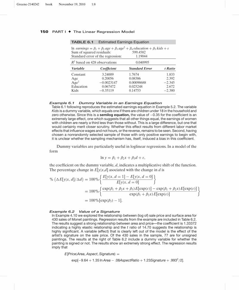
ln earnings = β1 + β2 age + β3 age2 + β4 education + β5 kids + εSum of squared residuals: 599.4582Standard error of the regression: 1.19044
R2 based on 428 observations 0.040995
Variable Coefficient Standard Error t Ratio
Constant 3.24009 1.7674 1.833Age 0.20056 0.08386 2.392Age2 −0.0023147 0.00098688 −2.345Education 0.067472 0.025248 2.672Kids −0.35119 0.14753 −2.380
Example 6.1 Dummy Variable in an Earnings EquationTable 6.1 following reproduces the estimated earnings equation in Example 5.2. The variableKids is a dummy variable, which equals one if there are children under 18 in the household andzero otherwise. Since this is a semilog equation, the value of −0.35 for the coefficient is anextremely large effect, one which suggests that all other things equal, the earnings of womenwith children are nearly a third less than those without. This is a large difference, but one thatwould certainly merit closer scrutiny. Whether this effect results from different labor marketeffects that influence wages and not hours, or the reverse, remains to be seen. Second, havingchosen a nonrandomly selected sample of those with only positive earnings to begin with,it is unclear whether the sampling mechanism has, itself, induced a bias in this coefficient.
Dummy variables are particularly useful in loglinear regressions. In a model of theform
ln y = β1 + β2x + β3d + ε,
the coefficient on the dummy variable, d, indicates a multiplicative shift of the function.The percentage change in E[y|x,d] asociated with the change in d is
%(�E[y|x, d]/�d
) = 100%{
E[y|x, d = 1] − E[y|x, d = 0]E[y|x, d = 0]
}= 100%
{exp(β1 + β2x + β3)E[exp(ε)] − exp(β1 + β2x)E[exp(ε)]
exp(β1 + β2x)E[exp(ε)]
}= 100%[exp(β3) − 1].
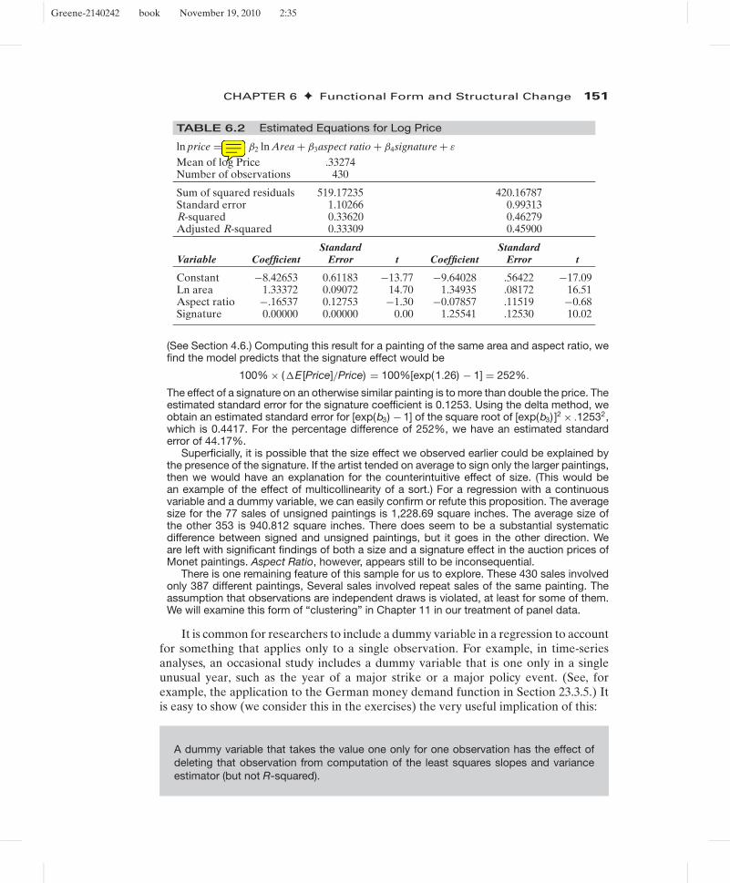
Example 6.2 Value of a SignatureIn Example 4.10 we explored the relationship between (log of) sale price and surface area for430 sales of Monet paintings. Regression results from the example are included in Table 6.2.The results suggest a strong relationship between area and price—the coefficient is 1.33372indicating a highly elastic relationship and the t ratio of 14.70 suggests the relationship ishighly significant. A variable (effect) that is clearly left out of the model is the effect of theartist’s signature on the sale price. Of the 430 sales in the sample, 77 are for unsignedpaintings. The results at the right of Table 6.2 include a dummy variable for whether thepainting is signed or not. The results show an extremely strong effect. The regression resultsimply that
E [Price|Area, Aspect, Signature) =exp[−9.64 + 1.35 ln Area − .08AspectRatio + 1.23Signature + .9932/2].
Greene-2140242 book November 19, 2010 2:35
CHAPTER 6 ✦ Functional Form and Structural Change 151
TABLE 6.2 Estimated Equations for Log Price
ln price = β1 + β2 ln Area + β3aspect ratio + β4signature + ε
Mean of log Price .33274Number of observations 430
Sum of squared residuals 519.17235 420.16787Standard error 1.10266 0.99313R-squared 0.33620 0.46279Adjusted R-squared 0.33309 0.45900
Standard StandardVariable Coefficient Error t Coefficient Error t
Constant −8.42653 0.61183 −13.77 −9.64028 .56422 −17.09Ln area 1.33372 0.09072 14.70 1.34935 .08172 16.51Aspect ratio −.16537 0.12753 −1.30 −0.07857 .11519 −0.68Signature 0.00000 0.00000 0.00 1.25541 .12530 10.02
(See Section 4.6.) Computing this result for a painting of the same area and aspect ratio, wefind the model predicts that the signature effect would be
100% × (�E [Price]/Price) = 100%[exp(1.26) − 1] = 252%.
The effect of a signature on an otherwise similar painting is to more than double the price. Theestimated standard error for the signature coefficient is 0.1253. Using the delta method, weobtain an estimated standard error for [exp(b3) − 1] of the square root of [exp(b3) ]2 × .12532,which is 0.4417. For the percentage difference of 252%, we have an estimated standarderror of 44.17%.
Superficially, it is possible that the size effect we observed earlier could be explained bythe presence of the signature. If the artist tended on average to sign only the larger paintings,then we would have an explanation for the counterintuitive effect of size. (This would bean example of the effect of multicollinearity of a sort.) For a regression with a continuousvariable and a dummy variable, we can easily confirm or refute this proposition. The averagesize for the 77 sales of unsigned paintings is 1,228.69 square inches. The average size ofthe other 353 is 940.812 square inches. There does seem to be a substantial systematicdifference between signed and unsigned paintings, but it goes in the other direction. Weare left with significant findings of both a size and a signature effect in the auction prices ofMonet paintings. Aspect Ratio, however, appears still to be inconsequential.
There is one remaining feature of this sample for us to explore. These 430 sales involvedonly 387 different paintings, Several sales involved repeat sales of the same painting. Theassumption that observations are independent draws is violated, at least for some of them.We will examine this form of “clustering” in Chapter 11 in our treatment of panel data.
It is common for researchers to include a dummy variable in a regression to accountfor something that applies only to a single observation. For example, in time-seriesanalyses, an occasional study includes a dummy variable that is one only in a singleunusual year, such as the year of a major strike or a major policy event. (See, forexample, the application to the German money demand function in Section 23.3.5.) Itis easy to show (we consider this in the exercises) the very useful implication of this:
A dummy variable that takes the value one only for one observation has the effect ofdeleting that observation from computation of the least squares slopes and varianceestimator (but not R-squared).
Greene-2140242 book November 19, 2010 1:8
152 PART I ✦ The Linear Regression Model
6.2.2 SEVERAL CATEGORIES
When there are several categories, a set of binary variables is necessary. Correctingfor seasonal factors in macroeconomic data is a common application. We could write aconsumption function for quarterly data as
Ct = β1 + β2xt + δ1 Dt1 + δ2 Dt2 + δ3 Dt3 + εt ,
where xt is disposable income. Note that only three of the four quarterly dummy vari-ables are included in the model. If the fourth were included, then the four dummyvariables would sum to one at every observation, which would reproduce the constantterm—a case of perfect multicollinearity. This is known as the dummy variable trap.Thus, to avoid the dummy variable trap, we drop the dummy variable for the fourth quar-ter. (Depending on the application, it might be preferable to have four separate dummyvariables and drop the overall constant.)1 Any of the four quarters (or 12 months) canbe used as the base period.
The preceding is a means of deseasonalizing the data. Consider the alternativeformulation:
Ct = βxt + δ1 Dt1 + δ2 Dt2 + δ3 Dt3 + δ4 Dt4 + εt . (6-1)
Using the results from Section 3.3 on partitioned regression, we know that the precedingmultiple regression is equivalent to first regressing C and x on the four dummy variablesand then using the residuals from these regressions in the subsequent regression ofdeseasonalized consumption on deseasonalized income. Clearly, deseasonalizing in thisfashion prior to computing the simple regression of consumption on income producesthe same coefficient on income (and the same vector of residuals) as including the setof dummy variables in the regression.
Example 6.3 Genre Effects on Movie Box Office ReceiptsTable 4.8 in Example 4.12 presents the results of the regression of log of box office receiptsfor 62 2009 movies on a number of variables including a set of dummy variables for genre:Action, Comedy, Animated, or Horror. The left out category is “any of the remaining 9 genres”in the standard set of 13 that is usually used in models such as this one. The four coefficientsare −.869, −.016, −.833, +.375, respectively. This suggests that, save for horror movies,these genres typically fare substantially worse at the box office than other types of movies.We note the use of b directly to estimate the percentage change for the category, as wedid in example 6.1 when we interpreted the coefficient of −.35 on Kids as indicative of a35 percent change in income, is an approximation that works well when b is close to zerobut deteriorates as it gets far from zero. Thus, the value of −.869 above does not translateto an 87 percent difference between Action movies and other movies. Using the formula weused in Example 6.2, we find an estimated difference closer to [exp(−.869) − 1] or about58 percent.
6.2.3 SEVERAL GROUPINGS
The case in which several sets of dummy variables are needed is much the same asthose we have already considered, with one important exception. Consider a model ofstatewide per capita expenditure on education y as a function of statewide per capitaincome x. Suppose that we have observations on all n = 50 states for T = 10 years.
1See Suits (1984) and Greene and Seaks (1991).
Greene-2140242 book November 19, 2010 1:8
CHAPTER 6 ✦ Functional Form and Structural Change 153
A regression model that allows the expected expenditure to change over time as wellas across states would be
yit = α + βxit + δi + θt + εi t . (6-2)
As before, it is necessary to drop one of the variables in each set of dummy variablesto avoid the dummy variable trap. For our example, if a total of 50 state dummies and10 time dummies is retained, a problem of “perfect multicollinearity” remains; the sumsof the 50 state dummies and the 10 time dummies are the same, that is, 1. One of thevariables in each of the sets (or the overall constant term and one of the variables inone of the sets) must be omitted.
Example 6.4 Analysis of CovarianceThe data in Appendix Table F6.1 were used in a study of efficiency in production of airlineservices in Greene (2007a). The airline industry has been a favorite subject of study [e.g.,Schmidt and Sickles (1984); Sickles, Good, and Johnson (1986)], partly because of interestin this rapidly changing market in a period of deregulation and partly because of an abun-dance of large, high-quality data sets collected by the (no longer existent) Civil AeronauticsBoard. The original data set consisted of 25 firms observed yearly for 15 years (1970 to 1984),a “balanced panel.” Several of the firms merged during this period and several others expe-rienced strikes, which reduced the number of complete observations substantially. Omittingthese and others because of missing data on some of the variables left a group of 10 fullobservations, from which we have selected six for the examples to follow. We will fit a costequation of the form
ln Ci ,t = β1 + β2 ln Qi ,t + β3 ln2 Qi ,t + β4 ln Pfuel i,t + β5 Loadfactori ,t
+14∑
t=1
θt Di ,t +5∑
i =1
δi Fi ,t + εi ,t .
The dummy variables are Di ,t which is the year variable and Fi ,t which is the firm variable. Wehave dropped the last one in each group. The estimated model for the full specification is
ln Ci ,t = 13.56 + 0.8866 ln Qi ,t + 0.01261 ln2 Qi ,t + 0.1281 ln Pf i ,t − 0.8855 LFi ,t
+ time effects + firm effects.
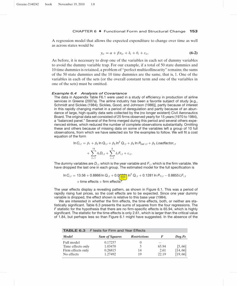
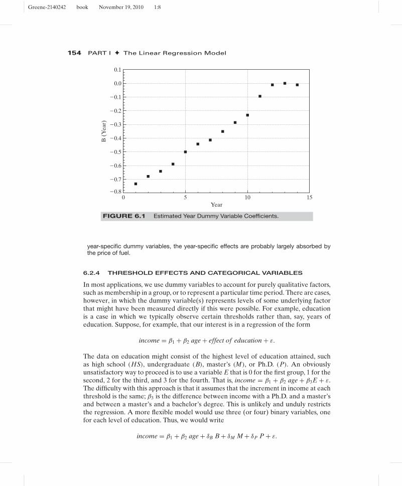
The year effects display a revealing pattern, as shown in Figure 6.1. This was a period ofrapidly rising fuel prices, so the cost effects are to be expected. Since one year dummyvariable is dropped, the effect shown is relative to this base year (1984).
We are interested in whether the firm effects, the time effects, both, or neither are sta-tistically significant. Table 6.3 presents the sums of squares from the four regressions. TheF statistic for the hypothesis that there are no firm-specific effects is 65.94, which is highlysignificant. The statistic for the time effects is only 2.61, which is larger than the critical valueof 1.84, but perhaps less so than Figure 6.1 might have suggested. In the absence of the
TABLE 6.3 F tests for Firm and Year Effects
Model Sum of Squares Restrictions F Deg.Fr.
Full model 0.17257 0 —Time effects only 1.03470 5 65.94 [5, 66]Firm effects only 0.26815 14 2.61 [14, 66]No effects 1.27492 19 22.19 [19, 66]
Greene-2140242 book November 19, 2010 1:8
154 PART I ✦ The Linear Regression Model
0.1
0.0
�0.1
�0.2
�0.3
�0.4
�0.5
�0.6
�0.7
�0.80 5
Year
B (
Yea
r)
10 15
FIGURE 6.1 Estimated Year Dummy Variable Coefficients.
year-specific dummy variables, the year-specific effects are probably largely absorbed bythe price of fuel.
6.2.4 THRESHOLD EFFECTS AND CATEGORICAL VARIABLES
In most applications, we use dummy variables to account for purely qualitative factors,such as membership in a group, or to represent a particular time period. There are cases,however, in which the dummy variable(s) represents levels of some underlying factorthat might have been measured directly if this were possible. For example, educationis a case in which we typically observe certain thresholds rather than, say, years ofeducation. Suppose, for example, that our interest is in a regression of the form
income = β1 + β2 age + effect of education + ε.
The data on education might consist of the highest level of education attained, suchas high school (HS), undergraduate (B), master’s (M), or Ph.D. (P). An obviouslyunsatisfactory way to proceed is to use a variable E that is 0 for the first group, 1 for thesecond, 2 for the third, and 3 for the fourth. That is, income = β1 + β2 age + β3E + ε.The difficulty with this approach is that it assumes that the increment in income at eachthreshold is the same; β3 is the difference between income with a Ph.D. and a master’sand between a master’s and a bachelor’s degree. This is unlikely and unduly restrictsthe regression. A more flexible model would use three (or four) binary variables, onefor each level of education. Thus, we would write
income = β1 + β2 age + δB B + δM M + δP P + ε.

Greene-2140242 book November 19, 2010 1:8
CHAPTER 6 ✦ Functional Form and Structural Change 155
The correspondence between the coefficients and income for a given age is
High school : E [income | age, HS] = β1 + β2 age,
Bachelor’s : E [income | age, B] = β1 + β2 age + δB,
Master’s : E [income | age, M] = β1 + β2 age + δM,
Ph.D. : E [income | age, P] = β1 + β2 age + δP.
The differences between, say, δP and δM and between δM and δB are of interest. Obvi-ously, these are simple to compute. An alternative way to formulate the equation thatreveals these differences directly is to redefine the dummy variables to be 1 if the indi-vidual has the degree, rather than whether the degree is the highest degree obtained.Thus, for someone with a Ph.D., all three binary variables are 1, and so on. By definingthe variables in this fashion, the regression is now
High school : E [income | age, HS] = β1 + β2 age,
Bachelor’s : E [income | age, B] = β1 + β2 age + δB,
Master’s : E [income | age, M] = β1 + β2 age + δB + δM,
Ph.D. : E [income | age, P] = β1 + β2 age + δB + δM + δP.
Instead of the difference between a Ph.D. and the base case, in this model δP is themarginal value of the Ph.D. How equations with dummy variables are formulated is amatter of convenience. All the results can be obtained from a basic equation.
6.2.5 TREATMENT EFFECTS AND DIFFERENCEIN DIFFERENCES REGRESSION
Researchers in many fields have studied the effect of a treatment on some kind ofresponse. Examples include the effect of going to college on lifetime income [Daleand Krueger (2002)], the effect of cash transfers on child health [Gertler (2004)], theeffect of participation in job training programs on income [LaLonde (1986)] and pre-versus postregime shifts in macroeconomic models [Mankiw (2006)], to name but afew. These examples can be formulated in regression models involving a single dummyvariable:
yi = xiβ + δDi + εi ,
where the shift parameter, δ, measures the impact of the treatment or the policy change(conditioned on x) on the sampled individuals. In the simplest case of a comparison ofone group to another,
yi = β1 + β2 Di + εi ,
we will have b1 = (y|Di = 0), that is, the average outcome of those who did not ex-perience the intervention, and b2 = (y|Di = 1) − (y|Di = 0), the difference in themeans of the two groups. In the Dale and Krueger (2002) study, the model comparedthe incomes of students who attended elite colleges to those who did not. When theanalysis is of an intervention that occurs over time, such as Krueger’s (1999) analysisof the Tennessee STAR experiment in which school performance measures were ob-served before and after a policy dictated a change in class sizes, the treatment dummy
Greene-2140242 book November 19, 2010 1:8
156 PART I ✦ The Linear Regression Model
variable will be a period indicator, Dt = 0 in period 1 and 1 in period 2. The effect in β2
measures the change in the outcome variable, for example, school performance, pre- topostintervention; b2 = y1 − y0.
The assumption that the treatment group does not change from period 1 to period 2weakens this comparison. A strategy for strengthening the result is to include in thesample a group of control observations that do not receive the treatment. The change inthe outcome for the treatment group can then be compared to the change for the controlgroup under the presumption that the difference is due to the intervention. An intriguingapplication of this strategy is often used in clinical trials for health interventions toaccommodate the placebo effect. The placebo “effect” is a controversial, but apparentlytangible outcome in some clinical trials in which subjects “respond” to the treatmenteven when the treatment is a decoy intervention, such as a sugar or starch pill in a drugtrial. [See Hrobjartsson and Peter C. Gotzsche, 2001]. A broad template for assessmentof the results of such a clinical trial is as follows: The subjects who receive the placeboare the controls. The outcome variable—level of cholesterol for example—is measuredat the baseline for both groups. The treatment group receives the drug; the controlgroup receives the placebo, and the outcome variable is measured posttreatment. Theimpact is measured by the difference in differences,
E = [(yexit|treatment) − (ybaseline|treatment)] − [(yexit|placebo) − (ybaseline|placebo)].
The presumption is that the difference in differences measurement is robust to theplacebo effect if it exists. If there is no placebo effect, the result is even stronger (assumingthere is a result).
An increasingly common social science application of treatment effect models withdummy variables is in the evaluation of the effects of discrete changes in policy.2 Apioneering application is the study of the Manpower Development and Training Act(MDTA) by Ashenfelter and Card (1985). The simplest form of the model is one witha pre- and posttreatment observation on a group, where the outcome variable is y,with
yit = β1 + β2Tt + β3 Di + β4Tt × Di + ε, t = 1, 2. (6-3)
In this model, Tt is a dummy variable that is zero in the pretreatment period andone after the treatment and Di equals one for those individuals who received the“treatment.” The change in the outcome variable for the “treated” individuals willbe
(yi2|Di = 1) − (yi1|Di = 1) = (β1 + β2 + β3 + β4) − (β1 + β3) = β2 + β4.
For the controls, this is
(yi2|Di = 0) − (yi1|Di = 0) = (β1 + β2) − (β1) = β2.
The difference in differences is
[(yi2|Di = 1) − (yi1|Di = 1)] − [(yi2|Di = 0) − (yi1|Di = 0)] = β4.
2Surveys of literatures on treatment effects, including use of D-i-D estimators, are provided by Imbens andWooldridge (2009) and Millimet, Smith, and Vytlacil (2008).
Greene-2140242 book November 19, 2010 1:8
CHAPTER 6 ✦ Functional Form and Structural Change 157
In the multiple regression of yit on a constant, T, D and TD, the least squares estimateof β4 will equal the difference in the changes in the means,
b4 = (y|D = 1, Period 2) − (y|D = 1, Period 1)
− (y|D = 0, Period 2) − (y|D = 0, Period 1)
= �y|treatment − �y|control.
The regression is called a difference in differences estimator in reference to this result.When the treatment is the result of a policy change or event that occurs completely
outside the context of the study, the analysis is often termed a natural experiment. Card’s(1990) study of a major immigration into Miami in 1979 discussed in Example 6.5 is anapplication.
Example 6.5 A Natural Experiment: The Mariel BoatliftA sharp change in policy can constitute a natural experiment. An example studied by Card(1990) is the Mariel boatlift from Cuba to Miami (May–September 1980) which increased theMiami labor force by 7 percent. The author examined the impact of this abrupt change in labormarket conditions on wages and employment for nonimmigrants. The model compared Miamito a similar city, Los Angeles. Let i denote an individual and D denote the “treatment,” whichfor an individual would be equivalent to “lived in a city that experienced the immigration.”For an individual in either Miami or Los Angeles, the outcome variable is
(Yi ) = 1 if they are unemployed and 0 if they are employed.
Let c denote the city and let t denote the period, before (1979) or after (1981) the immigration.Then, the unemployment rate in city c at time t is E [yi ,0|c, t] if there is no immigration and itis E [yi ,1|c, t] if there is the immigration. These rates are assumed to be constants. Then,
E [ yi ,0|c, t] = βt + γc without the immigration,
E [ yi ,1|c, t] = βt + γc + δ with the immigration.
The effect of the immigration on the unemployment rate is measured by δ. The natural ex-periment is that the immigration occurs in Miami and not in Los Angeles but is not a resultof any action by the people in either city. Then,
E [ yi |M, 79] = β79 + γM and E [ yi |M, 81] = β81 + γM + δ for Miami,
E [ yi |L, 79] = β79 + γL and E [ yi |L, 81] = β81 + γL for Los Angeles.
It is assumed that unemployment growth in the two cities would be the same if there wereno immigration. If neither city experienced the immigration, the change in the unemploymentrate would be
E [ yi ,0|M, 81] − E [ yi ,0|M, 79] = β81 − β79 for Miami,
E [ yi ,0|L, 81] − E [ yi ,0|L, 79] = β81 − β79 for Los Angeles.
If both cities were exposed to migration,
E [ yi ,1|M, 81] − E [ yi ,1|M, 79] = β81 − β79 + δ for Miami
E [ yi ,1|L, 81] − E [ yi ,1|L, 79] = β81 − β79 + δ for Los Angeles.
Only Miami experienced the migration (the “treatment”). The difference in differences thatquantifies the result of the experiment is
{E [ yi ,1|M, 81] − E [ yi ,1|M, 79]} − {E [ yi ,0|L, 81] − E [ yi ,0|L, 79]} = δ.
Greene-2140242 book November 19, 2010 1:8
158 PART I ✦ The Linear Regression Model
The author examined changes in employment rates and wages in the two cities over severalyears after the boatlift. The effects were surprisingly modest given the scale of the experimentin Miami.
One of the important issues in policy analysis concerns measurement of such treat-ment effects when the dummy variable results from an individual participation decision.In the clinical trial example given earlier, the control observations (it is assumed) do notknow they they are in the control group. The treatment assignment is exogenous to theexperiment. In contrast, in Keueger and Dale’s study, the assignment to the treatmentgroup, attended the elite college, is completely voluntary and determined by the indi-vidual. A crucial aspect of the analysis in this case is to accommodate the almost certainoutcome that the “treatment dummy” might be measuring the latent motivation andinitiative of the participants rather than the effect of the program itself. That is the mainappeal of the natural experiment approach—it more closely (possibly exactly) repli-cates the exogenous treatment assignment of a clinical trial.3 We will examine some ofthese cases in Chapters 8 and 18.
6.3 NONLINEARITY IN THE VARIABLES
It is useful at this point to write the linear regression model in a very general form: Letz = z1, z2, . . . , zL be a set of L independent variables; let f1, f2, . . . , fK be K linearlyindependent functions of z; let g(y) be an observable function of y; and retain the usualassumptions about the disturbance. The linear regression model is
g(y) = β1 f1(z) + β2 f2(z) + · · · + βK fK(z) + ε
= β1x1 + β2x2 + · · · + βKxK + ε
= x′β + ε.
(6-4)
By using logarithms, exponentials, reciprocals, transcendental functions, polynomials,products, ratios, and so on, this “linear” model can be tailored to any number ofsituations.
6.3.1 PIECEWISE LINEAR REGRESSION
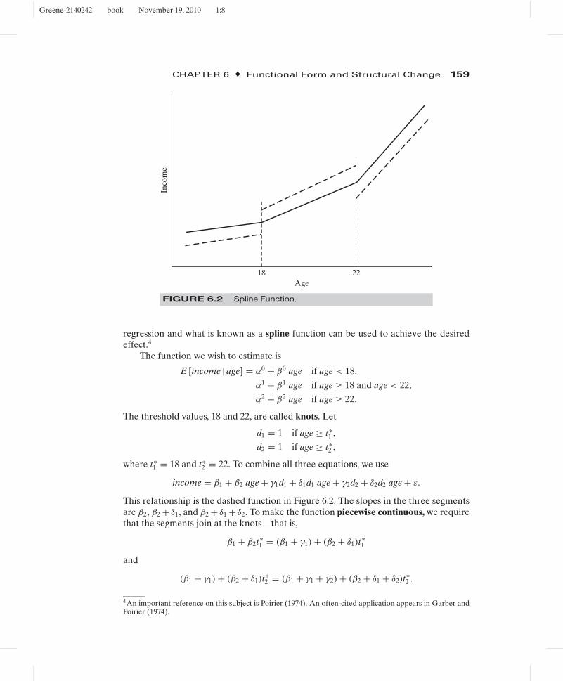
If one is examining income data for a large cross section of individuals of varying agesin a population, then certain patterns with regard to some age thresholds will be clearlyevident. In particular, throughout the range of values of age, income will be rising, but theslope might change at some distinct milestones, for example, at age 18, when the typicalindividual graduates from high school, and at age 22, when he or she graduates fromcollege. The time profile of income for the typical individual in this population mightappear as in Figure 6.2. Based on the discussion in the preceding paragraph, we couldfit such a regression model just by dividing the sample into three subsamples. However,this would neglect the continuity of the proposed function. The result would appearmore like the dotted figure than the continuous function we had in mind. Restricted
3See Angrist and Krueger (2001) and Angrist and Pischke (2010) for discussions of this approach.
Greene-2140242 book November 19, 2010 1:8
CHAPTER 6 ✦ Functional Form and Structural Change 159
18 22Age
Inco
me
FIGURE 6.2 Spline Function.
regression and what is known as a spline function can be used to achieve the desiredeffect.4
The function we wish to estimate is
E [income | age] = α0 + β0 age if age < 18,
α1 + β1 age if age ≥ 18 and age < 22,
α2 + β2 age if age ≥ 22.
The threshold values, 18 and 22, are called knots. Let
d1 = 1 if age ≥ t∗1 ,
d2 = 1 if age ≥ t∗2 ,
where t∗1 = 18 and t∗
2 = 22. To combine all three equations, we use
income = β1 + β2 age + γ1d1 + δ1d1 age + γ2d2 + δ2d2 age + ε.
This relationship is the dashed function in Figure 6.2. The slopes in the three segmentsare β2, β2 + δ1, and β2 + δ1 + δ2. To make the function piecewise continuous, we requirethat the segments join at the knots—that is,
β1 + β2t∗1 = (β1 + γ1) + (β2 + δ1)t∗
1
and
(β1 + γ1) + (β2 + δ1)t∗2 = (β1 + γ1 + γ2) + (β2 + δ1 + δ2)t∗
2 .
4An important reference on this subject is Poirier (1974). An often-cited application appears in Garber andPoirier (1974).
Greene-2140242 book November 19, 2010 1:8
160 PART I ✦ The Linear Regression Model
These are linear restrictions on the coefficients. Collecting terms, the first one is
γ1 + δ1t∗1 = 0 or γ1 = −δ1t∗
1 .
Doing likewise for the second and inserting these in (6-3), we obtain
income = β1 + β2 age + δ1d1 (age − t∗1 ) + δ2d2 (age − t∗
2 ) + ε.
Constrained least squares estimates are obtainable by multiple regression, using a con-stant and the variables
x1 = age,
x2 = age − 18 if age ≥ 18 and 0 otherwise,
andx3 = age − 22 if age ≥ 22 and 0 otherwise.
We can test the hypothesis that the slope of the function is constant with the joint testof the two restrictions δ1 = 0 and δ2 = 0.
6.3.2 FUNCTIONAL FORMS
A commonly used form of regression model is the loglinear model,
ln y = ln α +∑
k
βk ln Xk + ε = β1 +∑
k
βkxk + ε.
In this model, the coefficients are elasticities:(∂y∂ Xk
)(Xk
y
)= ∂ ln y
∂ ln Xk= βk. (6-5)
In the loglinear equation, measured changes are in proportional or percentage terms;βk measures the percentage change in y associated with a 1 percent change in Xk.This removes the units of measurement of the variables from consideration in using theregression model. An alternative approach sometimes taken is to measure the variablesand associated changes in standard deviation units. If the data are “standardized” beforeestimation using x∗
ik = (xik − xk)/sk and likewise for y, then the least squares regressioncoefficients measure changes in standard deviation units rather than natural units orpercentage terms. (Note that the constant term disappears from this regression.) It isnot necessary actually to transform the data to produce these results; multiplying eachleast squares coefficient bk in the original regression by sk/sy produces the same result.
A hybrid of the linear and loglinear models is the semilog equation
ln y = β1 + β2x + ε. (6-6)
We used this form in the investment equation in Section 5.2.2,
ln It = β1 + β2 (it − �pt ) + β3�pt + β4 ln Yt + β5t + εt ,
where the log of investment is modeled in the levels of the real interest rate, the pricelevel, and a time trend. In a semilog equation with a time trend such as this one,d ln I/dt = β5 is the average rate of growth of I. The estimated value of −0.00566 inTable 5.2 suggests that over the full estimation period, after accounting for all otherfactors, the average rate of growth of investment was −0.566 percent per year.
Greene-2140242 book November 19, 2010 1:8
CHAPTER 6 ✦ Functional Form and Structural Change 161
20 29 38 47Age
Ear
ning
s
3500
56 65
3000
2500
2000
1500
1000
500
FIGURE 6.3 Age-Earnings Profile.
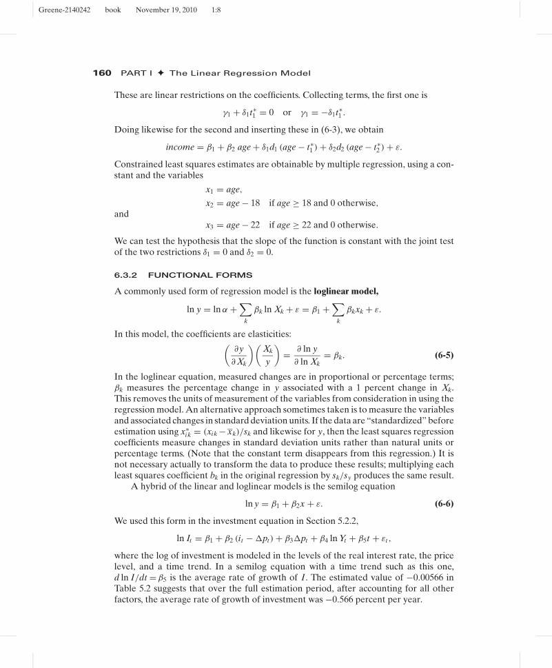
The coefficients in the semilog model are partial- or semi-elasticities; in (6-6), β2 is∂ ln y/∂x. This is a natural form for models with dummy variables such as the earningsequation in Example 5.2. The coefficient on Kids of −0.35 suggests that all else equal,earnings are approximately 35 percent less when there are children in the household.
The quadratic earnings equation in Example 6.1 shows another use of nonlineari-ties in the variables. Using the results in Example 6.1, we find that for a woman with12 years of schooling and children in the household, the age-earnings profile appears asin Figure 6.3. This figure suggests an important question in this framework. It is temptingto conclude that Figure 6.3 shows the earnings trajectory of a person at different ages,but that is not what the data provide. The model is based on a cross section, and what itdisplays is the earnings of different people of different ages. How this profile relates tothe expected earnings path of one individual is a different, and complicated question.
6.3.3 INTERACTION EFFECTS
Another useful formulation of the regression model is one with interaction terms. Forexample, a model relating braking distance D to speed S and road wetness W might be
D = β1 + β2S + β3W + β4SW + ε.
In this model,
∂ E [D | S, W]∂S
= β2 + β4W,
which implies that the marginal effect of higher speed on braking distance is increasedwhen the road is wetter (assuming that β4 is positive). If it is desired to form confidenceintervals or test hypotheses about these marginal effects, then the necessary standard
Greene-2140242 book November 19, 2010 1:8
162 PART I ✦ The Linear Regression Model
error is computed from
Var(
∂ E [D | S, W]∂S
)= Var[β2] + W2 Var[β4] + 2W Cov[β2, β4],
and similarly for ∂ E [D | S, W]/∂W. A value must be inserted for W. The sample meanis a natural choice, but for some purposes, a specific value, such as an extreme value ofW in this example, might be preferred.
6.3.4 IDENTIFYING NONLINEARITY
If the functional form is not known a priori, then there are a few approaches that mayhelp at least to identify any nonlinearity and provide some information about it from thesample. For example, if the suspected nonlinearity is with respect to a single regressorin the equation, then fitting a quadratic or cubic polynomial rather than a linear functionmay capture some of the nonlinearity. By choosing several ranges for the regressor inquestion and allowing the slope of the function to be different in each range, a piecewiselinear approximation to the nonlinear function can be fit.
Example 6.6 Functional Form for a Nonlinear Cost FunctionIn a celebrated study of economies of scale in the U.S. electric power industry, Nerlove (1963)analyzed the production costs of 145 American electricity generating companies. This studyproduced several innovations in microeconometrics. It was among the first major applicationsof statistical cost analysis. The theoretical development in Nerlove’s study was the first toshow how the fundamental theory of duality between production and cost functions could beused to frame an econometric model. Finally, Nerlove employed several useful techniquesto sharpen his basic model.
The focus of the paper was economies of scale, typically modeled as a characteristic ofthe production function. He chose a Cobb–Douglas function to model output as a functionof capital, K, labor, L, and fuel, F:
Q = α0 K αK LαL F αF eεi ,
where Q is output and εi embodies the unmeasured differences across firms. The economiesof scale parameter is r = αK +αL +αF . The value 1 indicates constant returns to scale. In thisstudy, Nerlove investigated the widely accepted assumption that producers in this industryenjoyed substantial economies of scale. The production model is loglinear, so assuming thatother conditions of the classical regression model are met, the four parameters could beestimated by least squares. However, he argued that the three factors could not be treatedas exogenous variables. For a firm that optimizes by choosing its factors of production, thedemand for fuel would be F ∗ = F ∗( Q, PK , PL , PF ) and likewise for labor and capital, socertainly the assumptions of the classical model are violated.
In the regulatory framework in place at the time, state commissions set rates and firmsmet the demand forthcoming at the regulated prices. Thus, it was argued that output (as wellas the factor prices) could be viewed as exogenous to the firm and, based on an argument byZellner, Kmenta, and Dreze (1966), Nerlove argued that at equilibrium, the deviation of costsfrom the long-run optimum would be independent of output. (This has a testable implicationwhich we will explore in Chapter 8.) Thus, the firm’s objective was cost minimization subjectto the constraint of the production function. This can be formulated as a Lagrangean problem,
MinK ,L ,F PK K + PL L + PF F + λ( Q − α0 K αK LαL F αF ) .
The solution to this minimization problem is the three factor demands and the multiplier(which measures marginal cost). Inserted back into total costs, this produces an (intrinsically
Greene-2140242 book November 19, 2010 1:8
CHAPTER 6 ✦ Functional Form and Structural Change 163
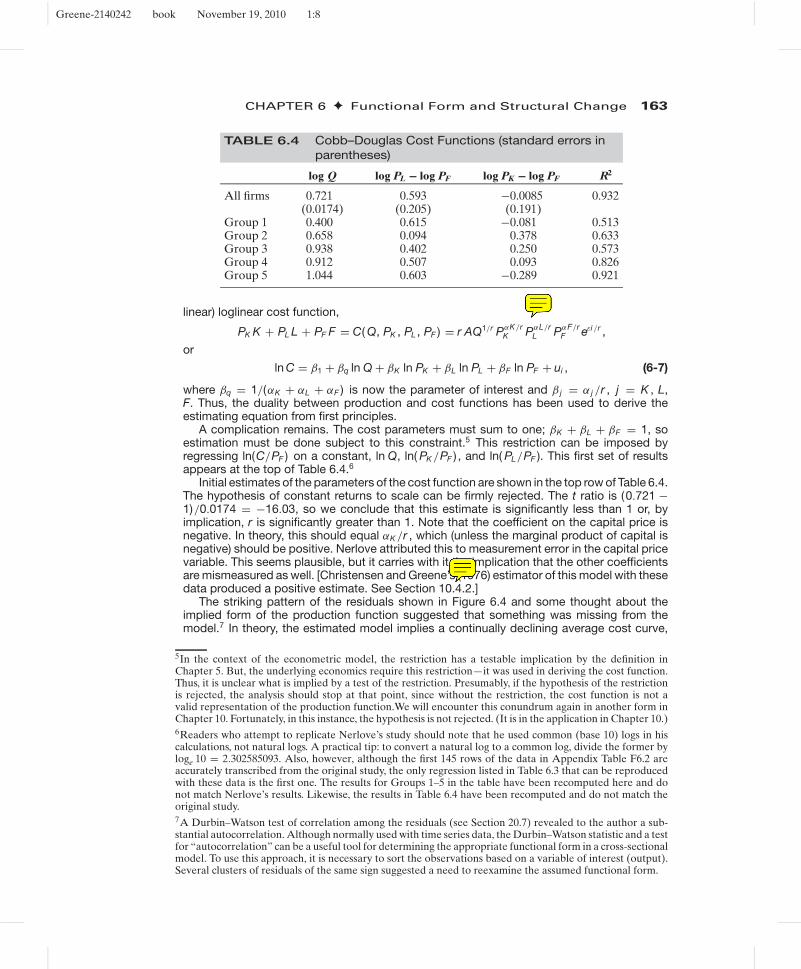
TABLE 6.4 Cobb–Douglas Cost Functions (standard errors inparentheses)
log Q log PL − log PF log PK − log PF R2
All firms 0.721 0.593 −0.0085 0.932(0.0174) (0.205) (0.191)
Group 1 0.400 0.615 −0.081 0.513Group 2 0.658 0.094 0.378 0.633Group 3 0.938 0.402 0.250 0.573Group 4 0.912 0.507 0.093 0.826Group 5 1.044 0.603 −0.289 0.921
linear) loglinear cost function,
PK K + PL L + PF F = C( Q, PK , PL , PF ) = r AQ1/r PαK/rK PαL/r
L PαF/rF eεi /r ,
or
ln C = β1 + βq ln Q + βK ln PK + βL ln PL + βF ln PF + ui , (6-7)
where βq = 1/(αK + αL + αF ) is now the parameter of interest and β j = α j /r , j = K , L,F. Thus, the duality between production and cost functions has been used to derive theestimating equation from first principles.
A complication remains. The cost parameters must sum to one; βK + βL + βF = 1, soestimation must be done subject to this constraint.5 This restriction can be imposed byregressing ln(C/PF ) on a constant, ln Q, ln( PK /PF ) , and ln( PL/PF ). This first set of resultsappears at the top of Table 6.4.6
Initial estimates of the parameters of the cost function are shown in the top row of Table 6.4.The hypothesis of constant returns to scale can be firmly rejected. The t ratio is (0.721 −1)/0.0174 = −16.03, so we conclude that this estimate is significantly less than 1 or, byimplication, r is significantly greater than 1. Note that the coefficient on the capital price isnegative. In theory, this should equal αK /r , which (unless the marginal product of capital isnegative) should be positive. Nerlove attributed this to measurement error in the capital pricevariable. This seems plausible, but it carries with it the implication that the other coefficientsare mismeasured as well. [Christensen and Greene’s (1976) estimator of this model with thesedata produced a positive estimate. See Section 10.4.2.]
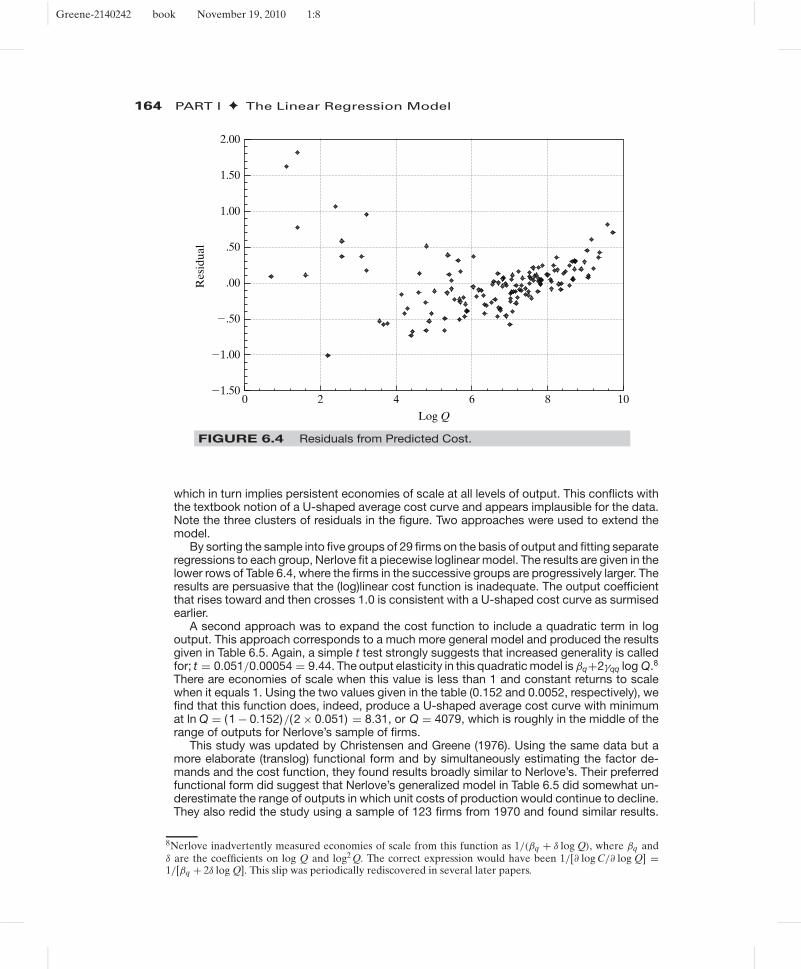
The striking pattern of the residuals shown in Figure 6.4 and some thought about theimplied form of the production function suggested that something was missing from themodel.7 In theory, the estimated model implies a continually declining average cost curve,
5In the context of the econometric model, the restriction has a testable implication by the definition inChapter 5. But, the underlying economics require this restriction—it was used in deriving the cost function.Thus, it is unclear what is implied by a test of the restriction. Presumably, if the hypothesis of the restrictionis rejected, the analysis should stop at that point, since without the restriction, the cost function is not avalid representation of the production function.We will encounter this conundrum again in another form inChapter 10. Fortunately, in this instance, the hypothesis is not rejected. (It is in the application in Chapter 10.)6Readers who attempt to replicate Nerlove’s study should note that he used common (base 10) logs in hiscalculations, not natural logs. A practical tip: to convert a natural log to a common log, divide the former byloge 10 = 2.302585093. Also, however, although the first 145 rows of the data in Appendix Table F6.2 areaccurately transcribed from the original study, the only regression listed in Table 6.3 that can be reproducedwith these data is the first one. The results for Groups 1–5 in the table have been recomputed here and donot match Nerlove’s results. Likewise, the results in Table 6.4 have been recomputed and do not match theoriginal study.7A Durbin–Watson test of correlation among the residuals (see Section 20.7) revealed to the author a sub-stantial autocorrelation. Although normally used with time series data, the Durbin–Watson statistic and a testfor “autocorrelation” can be a useful tool for determining the appropriate functional form in a cross-sectionalmodel. To use this approach, it is necessary to sort the observations based on a variable of interest (output).Several clusters of residuals of the same sign suggested a need to reexamine the assumed functional form.
Greene-2140242 book November 19, 2010 1:8
164 PART I ✦ The Linear Regression Model
Log Q
�1.00
�.50
.00
.50
1.00
1.50
2.00
�1.502 4 6 8 100
Res
idua
l
FIGURE 6.4 Residuals from Predicted Cost.
which in turn implies persistent economies of scale at all levels of output. This conflicts withthe textbook notion of a U-shaped average cost curve and appears implausible for the data.Note the three clusters of residuals in the figure. Two approaches were used to extend themodel.
By sorting the sample into five groups of 29 firms on the basis of output and fitting separateregressions to each group, Nerlove fit a piecewise loglinear model. The results are given in thelower rows of Table 6.4, where the firms in the successive groups are progressively larger. Theresults are persuasive that the (log)linear cost function is inadequate. The output coefficientthat rises toward and then crosses 1.0 is consistent with a U-shaped cost curve as surmisedearlier.
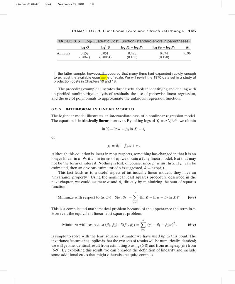
A second approach was to expand the cost function to include a quadratic term in logoutput. This approach corresponds to a much more general model and produced the resultsgiven in Table 6.5. Again, a simple t test strongly suggests that increased generality is calledfor; t = 0.051/0.00054 = 9.44. The output elasticity in this quadratic model is βq+2γqq log Q.8
There are economies of scale when this value is less than 1 and constant returns to scalewhen it equals 1. Using the two values given in the table (0.152 and 0.0052, respectively), wefind that this function does, indeed, produce a U-shaped average cost curve with minimumat ln Q = (1 − 0.152)/(2 × 0.051) = 8.31, or Q = 4079, which is roughly in the middle of therange of outputs for Nerlove’s sample of firms.
This study was updated by Christensen and Greene (1976). Using the same data but amore elaborate (translog) functional form and by simultaneously estimating the factor de-mands and the cost function, they found results broadly similar to Nerlove’s. Their preferredfunctional form did suggest that Nerlove’s generalized model in Table 6.5 did somewhat un-derestimate the range of outputs in which unit costs of production would continue to decline.They also redid the study using a sample of 123 firms from 1970 and found similar results.
8Nerlove inadvertently measured economies of scale from this function as 1/(βq + δ log Q), where βq andδ are the coefficients on log Q and log2 Q. The correct expression would have been 1/[∂ log C/∂ log Q] =1/[βq + 2δ log Q]. This slip was periodically rediscovered in several later papers.
Greene-2140242 book November 19, 2010 1:8
CHAPTER 6 ✦ Functional Form and Structural Change 165
TABLE 6.5 Log-Quadratic Cost Function (standard errors in parentheses)
log Q log2 Q log PL − log PF log PK − log PF R2
All firms 0.152 0.051 0.481 0.074 0.96(0.062) (0.0054) (0.161) (0.150)
In the latter sample, however, it appeared that many firms had expanded rapidly enoughto exhaust the available economies of scale. We will revisit the 1970 data set in a study ofproduction costs in Chapters 10 and 18.
The preceding example illustrates three useful tools in identifying and dealing withunspecified nonlinearity: analysis of residuals, the use of piecewise linear regression,and the use of polynomials to approximate the unknown regression function.
6.3.5 INTRINSICALLY LINEAR MODELS
The loglinear model illustrates an intermediate case of a nonlinear regression model.The equation is intrinsically linear, however. By taking logs of Yi = αXβ2
i eεi , we obtain
ln Yi = ln α + β2 ln Xi + εi
or
yi = β1 + β2xi + εi .
Although this equation is linear in most respects, something has changed in that it is nolonger linear in α. Written in terms of β1, we obtain a fully linear model. But that maynot be the form of interest. Nothing is lost, of course, since β1 is just ln α. If β1 can beestimated, then an obvious estimator of α is suggested, α = exp(b1).
This fact leads us to a useful aspect of intrinsically linear models; they have an“invariance property.” Using the nonlinear least squares procedure described in thenext chapter, we could estimate α and β2 directly by minimizing the sum of squaresfunction;
Minimize with respect to (α, β2) : S(α, β2) =n∑
i=1
(ln Yi − ln α − β2 ln Xi )2 . (6-8)
This is a complicated mathematical problem because of the appearance the term ln α.However, the equivalent linear least squares problem,
Minimize with respect to (β1, β2) : S(β1, β2) =n∑
i=1
(yi − β1 − β2xi )2 , (6-9)
is simple to solve with the least squares estimator we have used up to this point. Theinvariance feature that applies is that the two sets of results will be numerically identical;we will get the identical result from estimating α using (6-8) and from using exp(β1) from(6-9). By exploiting this result, we can broaden the definition of linearity and includesome additional cases that might otherwise be quite complex.
Greene-2140242 book November 19, 2010 1:8
166 PART I ✦ The Linear Regression Model
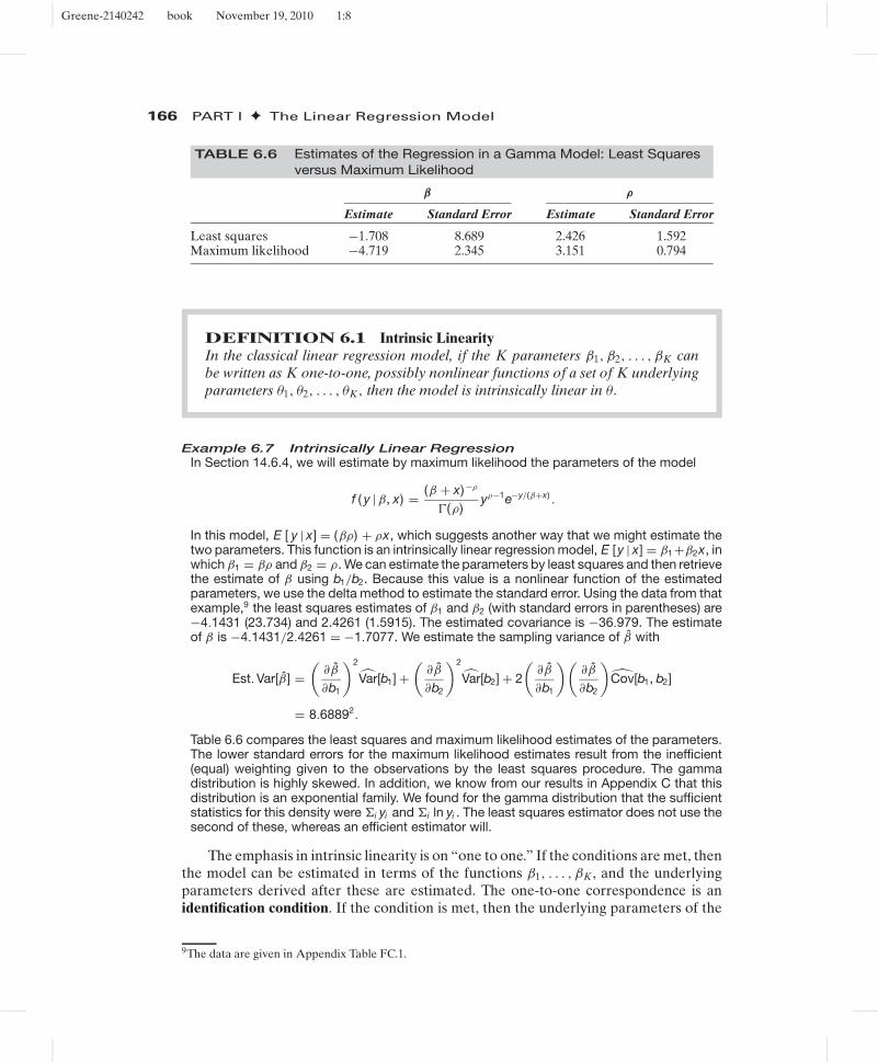
TABLE 6.6 Estimates of the Regression in a Gamma Model: Least Squaresversus Maximum Likelihood
β ρ
Estimate Standard Error Estimate Standard Error
Least squares −1.708 8.689 2.426 1.592Maximum likelihood −4.719 2.345 3.151 0.794
DEFINITION 6.1 Intrinsic LinearityIn the classical linear regression model, if the K parameters β1, β2, . . . , βK canbe written as K one-to-one, possibly nonlinear functions of a set of K underlyingparameters θ1, θ2, . . . , θK, then the model is intrinsically linear in θ .
Example 6.7 Intrinsically Linear RegressionIn Section 14.6.4, we will estimate by maximum likelihood the parameters of the model
f ( y | β, x) = (β + x)−ρ
�(ρ)yρ−1e−y/(β+x) .
In this model, E [ y | x] = (βρ) + ρx, which suggests another way that we might estimate thetwo parameters. This function is an intrinsically linear regression model, E [y | x] = β1+β2x, inwhich β1 = βρ and β2 = ρ. We can estimate the parameters by least squares and then retrievethe estimate of β using b1/b2. Because this value is a nonlinear function of the estimatedparameters, we use the delta method to estimate the standard error. Using the data from thatexample,9 the least squares estimates of β1 and β2 (with standard errors in parentheses) are−4.1431 (23.734) and 2.4261 (1.5915). The estimated covariance is −36.979. The estimateof β is −4.1431/2.4261 = −1.7077. We estimate the sampling variance of β with
Est. Var[β] =(
∂β
∂b1
)2
Var[b1] +(
∂β
∂b2
)2
Var[b2] + 2
(∂β
∂b1
)(∂β
∂b2
)Cov[b1, b2]
= 8.68892.
Table 6.6 compares the least squares and maximum likelihood estimates of the parameters.The lower standard errors for the maximum likelihood estimates result from the inefficient(equal) weighting given to the observations by the least squares procedure. The gammadistribution is highly skewed. In addition, we know from our results in Appendix C that thisdistribution is an exponential family. We found for the gamma distribution that the sufficientstatistics for this density were i yi and i ln yi . The least squares estimator does not use thesecond of these, whereas an efficient estimator will.
The emphasis in intrinsic linearity is on “one to one.” If the conditions are met, thenthe model can be estimated in terms of the functions β1, . . . , βK, and the underlyingparameters derived after these are estimated. The one-to-one correspondence is anidentification condition. If the condition is met, then the underlying parameters of the
9The data are given in Appendix Table FC.1.
Greene-2140242 book November 19, 2010 1:8
CHAPTER 6 ✦ Functional Form and Structural Change 167
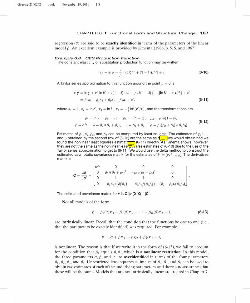
regression (θ) are said to be exactly identified in terms of the parameters of the linearmodel β. An excellent example is provided by Kmenta (1986, p. 515, and 1967).
Example 6.8 CES Production FunctionThe constant elasticity of substitution production function may be written
ln y = ln γ − ν
ρln[δK −ρ + (1 − δ) L−ρ ] + ε. (6-10)
A Taylor series approximation to this function around the point ρ = 0 is
ln y = ln γ + νδ ln K + ν(1 − δ) ln L + ρνδ(1 − δ){− 1
2 [ln K − ln L ]2} + ε′
= β1x1 + β2x2 + β3x3 + β4x4 + ε′, (6-11)
where x1 = 1, x2 = ln K , x3 = ln L , x4 = − 12 ln2( K/L ) , and the transformations are
β1 = ln γ , β2 = νδ, β3 = ν(1 − δ) , β4 = ρνδ(1 − δ) ,
γ = eβ1 , δ = β2/(β2 + β3) , ν = β2 + β3, ρ = β4(β2 + β3)/(β2β3) .(6-12)
Estimates of β1, β2, β3, and β4 can be computed by least squares. The estimates of γ , δ, ν,and ρ obtained by the second row of (6-12) are the same as those we would obtain had wefound the nonlinear least squares estimates of (6-11) directly. As Kmenta shows, however,they are not the same as the nonlinear least squares estimates of (6-10) due to the use of theTaylor series approximation to get to (6-11). We would use the delta method to construct theestimated asymptotic covariance matrix for the estimates of θ ′ = [γ , δ, ν, ρ]. The derivativesmatrix is
C = ∂θ
∂β ′ =
⎡⎢⎢⎣eβ1 0 0 0
0 β3/(β2 + β3) 2 −β2/(β2 + β3) 2 00 1 1 0
0 −β3β4
/(β2
2β3
) −β2β4
/(β2β
23
)(β2 + β3)/(β2β3)
⎤⎥⎥⎦ .
The estimated covariance matrix for θ is C [s2(X′X)−1]C′.
Not all models of the form
yi = β1(θ)xi1 + β2(θ)xi2 + · · · + βK(θ)xik + εi (6-13)
are intrinsically linear. Recall that the condition that the functions be one to one (i.e.,that the parameters be exactly identified) was required. For example,
yi = α + βxi1 + γ xi2 + βγ xi3 + εi
is nonlinear. The reason is that if we write it in the form of (6-13), we fail to accountfor the condition that β4 equals β2β3, which is a nonlinear restriction. In this model,the three parameters α, β, and γ are overidentified in terms of the four parametersβ1, β2, β3, and β4. Unrestricted least squares estimates of β2, β3, and β4 can be used toobtain two estimates of each of the underlying parameters, and there is no assurance thatthese will be the same. Models that are not intrinsically linear are treated in Chapter 7.
Greene-2140242 book November 19, 2010 1:8
168 PART I ✦ The Linear Regression Model
150
125
100
75
50
25
00.250 0.300 0.350 0.400 0.450
G0.500 0.550 0.6500.600
PG
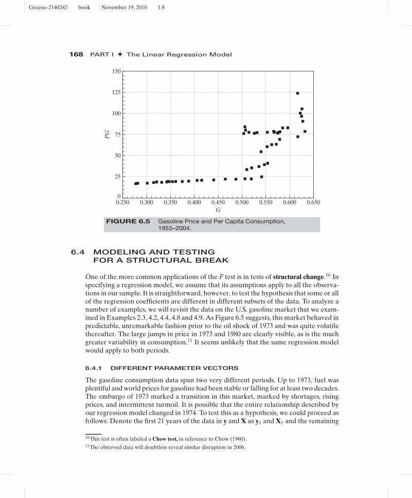
FIGURE 6.5 Gasoline Price and Per Capita Consumption,1953–2004.
6.4 MODELING AND TESTINGFOR A STRUCTURAL BREAK
One of the more common applications of the F test is in tests of structural change.10 Inspecifying a regression model, we assume that its assumptions apply to all the observa-tions in our sample. It is straightforward, however, to test the hypothesis that some or allof the regression coefficients are different in different subsets of the data. To analyze anumber of examples, we will revisit the data on the U.S. gasoline market that we exam-ined in Examples 2.3, 4.2, 4.4, 4.8 and 4.9. As Figure 6.5 suggests, this market behaved inpredictable, unremarkable fashion prior to the oil shock of 1973 and was quite volatilethereafter. The large jumps in price in 1973 and 1980 are clearly visible, as is the muchgreater variability in consumption.11 It seems unlikely that the same regression modelwould apply to both periods.
6.4.1 DIFFERENT PARAMETER VECTORS
The gasoline consumption data span two very different periods. Up to 1973, fuel wasplentiful and world prices for gasoline had been stable or falling for at least two decades.The embargo of 1973 marked a transition in this market, marked by shortages, risingprices, and intermittent turmoil. It is possible that the entire relationship described byour regression model changed in 1974. To test this as a hypothesis, we could proceed asfollows: Denote the first 21 years of the data in y and X as y1 and X1 and the remaining
10This test is often labeled a Chow test, in reference to Chow (1960).11The observed data will doubtless reveal similar disruption in 2006.
Greene-2140242 book November 19, 2010 1:8
CHAPTER 6 ✦ Functional Form and Structural Change 169
years as y2 and X2. An unrestricted regression that allows the coefficients to be differentin the two periods is [
y1
y2
]=
[X1 00 X2
][β1β2
]+
[ε1
ε2
]. (6-14)
Denoting the data matrices as y and X, we find that the unrestricted least squaresestimator is
b = (X′X)−1X′y =[
X′1X1 00 X′
2X2
]−1[X′1y1
X′2y2
]=
[b1
b2
], (6-15)
which is least squares applied to the two equations separately. Therefore, the total sumof squared residuals from this regression will be the sum of the two residual sums ofsquares from the two separate regressions:
e′e = e′1e1 + e′
2e2.
The restricted coefficient vector can be obtained in two ways. Formally, the restrictionβ1 = β2 is Rβ = q, where R = [I : −I] and q = 0. The general result given earlier canbe applied directly. An easier way to proceed is to build the restriction directly into themodel. If the two coefficient vectors are the same, then (6-14) may be written[
y1
y2
]=
[X1
X2
]β +
[ε1
ε2
],
and the restricted estimator can be obtained simply by stacking the data and estimatinga single regression. The residual sum of squares from this restricted regression, e′
∗e∗,then forms the basis for the test. The test statistic is then given in (5-16), where J , thenumber of restrictions, is the number of columns in X2 and the denominator degrees offreedom is n1 + n2 − 2k.
6.4.2 INSUFFICIENT OBSERVATIONS
In some circumstances, the data series are not long enough to estimate one or theother of the separate regressions for a test of structural change. For example, one mightsurmise that consumers took a year or two to adjust to the turmoil of the two oil priceshocks in 1973 and 1979, but that the market never actually fundamentally changed orthat it only changed temporarily. We might consider the same test as before, but nowonly single out the four years 1974, 1975, 1980, and 1981 for special treatment. Becausethere are six coefficients to estimate but only four observations, it is not possible to fitthe two separate models. Fisher (1970) has shown that in such a circumstance, a validway to proceed is as follows:
1. Estimate the regression, using the full data set, and compute the restricted sum ofsquared residuals, e′
∗e∗.2. Use the longer (adequate) subperiod (n1 observations) to estimate the regression,
and compute the unrestricted sum of squares, e′1e1. This latter computation is done
assuming that with only n2 < K observations, we could obtain a perfect fit and thuscontribute zero to the sum of squares.
Greene-2140242 book November 19, 2010 1:8
170 PART I ✦ The Linear Regression Model
3. The F statistic is then computed, using
F [n2, n1 − K] = (e′∗e∗ − e′
1e1)/n2
e′1e1/(n1 − K)
. (6-16)
Note that the numerator degrees of freedom is n2, not K.12 This test has been labeledthe Chow predictive test because it is equivalent to extending the restricted model tothe shorter subperiod and basing the test on the prediction errors of the model in thislatter period.
6.4.3 CHANGE IN A SUBSET OF COEFFICIENTS
The general formulation previously suggested lends itself to many variations that allowa wide range of possible tests. Some important particular cases are suggested by ourgasoline market data. One possible description of the market is that after the oil shockof 1973, Americans simply reduced their consumption of gasoline by a fixed proportion,but other relationships in the market, such as the income elasticity, remained unchanged.This case would translate to a simple shift downward of the loglinear regression modelor a reduction only in the constant term. Thus, the unrestricted equation has separatecoefficients in the two periods, while the restricted equation is a pooled regression withseparate constant terms. The regressor matrices for these two cases would be of theform
(unrestricted) XU =[
i 0 Wpre73 0
0 i 0 Wpost73
]and
(restricted) XR =[
i 0 Wpre73
0 i Wpost73
].
The first two columns of XU are dummy variables that indicate the subperiod in whichthe observation falls.
Another possibility is that the constant and one or more of the slope coefficientschanged, but the remaining parameters remained the same. The results in Example 6.9suggest that the constant term and the price and income elasticities changed muchmore than the cross-price elasticities and the time trend. The Chow test for this typeof restriction looks very much like the one for the change in the constant term alone.Let Z denote the variables whose coefficients are believed to have changed, and let Wdenote the variables whose coefficients are thought to have remained constant. Then,the regressor matrix in the constrained regression would appear as
X =[
ipre Zpre 0 0 Wpre
0 0 ipost Zpost Wpost
]. (6-17)
As before, the unrestricted coefficient vector is the combination of the two separateregressions.
12One way to view this is that only n2 < K coefficients are needed to obtain this perfect fit.
Greene-2140242 book November 19, 2010 1:8
CHAPTER 6 ✦ Functional Form and Structural Change 171
6.4.4 TESTS OF STRUCTURAL BREAK WITHUNEQUAL VARIANCES
An important assumption made in using the Chow test is that the disturbance varianceis the same in both (or all) regressions. In the restricted model, if this is not true, the firstn1 elements of ε have variance σ 2
1 , whereas the next n2 have variance σ 22 , and so on. The
restricted model is, therefore, heteroscedastic, and our results for the classical regressionmodel no longer apply. As analyzed by Schmidt and Sickles (1977), Ohtani and Toyoda(1985), and Toyoda and Ohtani (1986), it is quite likely that the actual probability ofa type I error will be larger than the significance level we have chosen. (That is, weshall regard as large an F statistic that is actually less than the appropriate but unknowncritical value.) Precisely how severe this effect is going to be will depend on the dataand the extent to which the variances differ, in ways that are not likely to be obvious.
If the sample size is reasonably large, then we have a test that is valid whether ornot the disturbance variances are the same. Suppose that θ1 and θ2 are two consistentand asymptotically normally distributed estimators of a parameter based on indepen-dent samples,13 with asymptotic covariance matrices V1 and V2. Then, under the nullhypothesis that the true parameters are the same,
θ1 − θ2 has mean 0 and asymptotic covariance matrix V1 + V2.
Under the null hypothesis, the Wald statistic,
W = (θ1 − θ2)′(V1 + V2)
−1(θ1 − θ2), (6-18)
has a limiting chi-squared distribution with K degrees of freedom. A test that the differ-ence between the parameters is zero can be based on this statistic.14 It is straightforwardto apply this to our test of common parameter vectors in our regressions. Large valuesof the statistic lead us to reject the hypothesis.
In a small or moderately sized sample, the Wald test has the unfortunate propertythat the probability of a type I error is persistently larger than the critical level weuse to carry it out. (That is, we shall too frequently reject the null hypothesis that theparameters are the same in the subsamples.) We should be using a larger critical value.Ohtani and Kobayashi (1986) have devised a “bounds” test that gives a partial remedyfor the problem.15
It has been observed that the size of the Wald test may differ from what we haveassumed, and that the deviation would be a function of the alternative hypothesis. Thereare two general settings in which a test of this sort might be of interest. For comparingtwo possibly different populations—such as the labor supply equations for men versuswomen—not much more can be said about the suggested statistic in the absence ofspecific information about the alternative hypothesis. But a great deal of work on thistype of statistic has been done in the time-series context. In this instance, the nature ofthe alternative is rather more clearly defined.
13Without the required independence, this test and several similar ones will fail completely. The problembecomes a variant of the famous Behrens–Fisher problem.14See Andrews and Fair (1988). The true size of this suggested test is uncertain. It depends on the nature of thealternative. If the variances are radically different, the assumed critical values might be somewhat unreliable.15See also Kobayashi (1986). An alternative, somewhat more cumbersome test is proposed by Jayatissa (1977).Further discussion is given in Thursby (1982).
Greene-2140242 book November 19, 2010 1:8
172 PART I ✦ The Linear Regression Model
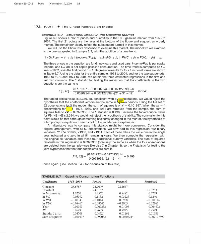
Example 6.9 Structural Break in the Gasoline MarketFigure 6.5 shows a plot of prices and quantities in the U.S. gasoline market from 1953 to2004. The first 21 points are the layer at the bottom of the figure and suggest an orderlymarket. The remainder clearly reflect the subsequent turmoil in this market.
We will use the Chow tests described to examine this market. The model we will examineis the one suggested in Example 2.3, with the addition of a time trend:
ln(G/Pop) t = β1 + β2 ln( Income/Pop) t + β3 ln PGt + β4 ln PNCt + β5 ln PUCt + β6t + εt .
The three prices in the equation are for G, new cars and used cars. Income/Pop is per capitaIncome, and G/Pop is per capita gasoline consumption. The time trend is computed as t =Year −1952, so in the first period t = 1. Regression results for four functional forms are shownin Table 6.7. Using the data for the entire sample, 1953 to 2004, and for the two subperiods,1953 to 1973 and 1974 to 2004, we obtain the three estimated regressions in the first andlast two columns. The F statistic for testing the restriction that the coefficients in the twoequations are the same is
F [6, 40] = (0.101997 − (0.00202244 + 0.007127899) )/6(0.00202244 + 0.007127899)/(21 + 31 − 12)
= 67.645.
The tabled critical value is 2.336, so, consistent with our expectations, we would reject thehypothesis that the coefficient vectors are the same in the two periods. Using the full set of52 observations to fit the model, the sum of squares is e∗′e∗ = 0.101997. When the n2 = 4observations for 1974, 1975, 1980, and 1981 are removed from the sample, the sum ofsquares falls to e′e = 0.0973936. The F statistic is 0.496. Because the tabled critical valuefor F [4, 48−6] is 2.594, we would not reject the hypothesis of stability. The conclusion to thispoint would be that although something has surely changed in the market, the hypothesis ofa temporary disequilibrium seems not to be an adequate explanation.
An alternative way to compute this statistic might be more convenient. Consider theoriginal arrangement, with all 52 observations. We now add to this regression four binaryvariables, Y1974, Y1975, Y1980, and Y1981. Each of these takes the value one in the singleyear indicated and zero in all 51 remaining years. We then compute the regression withthe original six variables and these four additional dummy variables. The sum of squaredresiduals in this regression is 0.0973936 (precisely the same as when the four observationsare deleted from the sample—see Exercise 7 in Chapter 3), so the F statistic for testing thejoint hypothesis that the four coefficients are zero is
F [4, 42] = (0.101997 − 0.0973936)/40.0973936/(52 − 6 − 4)
= 0.496
once again. (See Section 6.4.2 for discussion of this test.)
TABLE 6.7 Gasoline Consumption Functions
Coefficients 1953–2004 Pooled Preshock Postshock
Constant −26.6787 −24.9009 −22.1647Constant −24.8167 −15.3283ln Income/Pop 1.6250 1.4562 0.8482 0.3739ln PG −0.05392 −0.1132 −0.03227 −0.1240ln PNC −0.08343 −0.1044 0.6988 −0.001146ln PUC −0.08467 −0.08646 −0.2905 −0.02167Year −0.01393 −0.009232 0.01006 0.004492R2 0.9649 0.9683 0.9975 0.9529Standard error 0.04709 0.04524 0.01161 0.01689Sum of squares 0.101997 0.092082 0.00202244 0.007127899

Greene-2140242 book November 19, 2010 1:8
CHAPTER 6 ✦ Functional Form and Structural Change 173
The F statistic for testing the restriction that the coefficients in the two equations are thesame apart from the constant term is based on the last three sets of results in the table:
F [5, 40] = (0.092082 − (0.00202244 + 0.007127899) )/5(0.00202244 + 0.007127899)/(21 + 31 − 12)
= 72.506.
The tabled critical value is 2.449, so this hypothesis is rejected as well. The data suggestthat the models for the two periods are systematically different, beyond a simple shift in theconstant term.
The F ratio that results from estimating the model subject to the restriction that the twoautomobile price elasticities and the coefficient on the time trend are unchanged is
F [3, 40] = (0.01441975 − (0.00202244 + 0.007127899) )/3(0.00202244 + 0.007127899)/(52 − 6 − 6)
= 7.678.
(The restricted regression is not shown.) The critical value from the F table is 2.839, so thishypothesis is rejected as well. Note, however, that this value is far smaller than those weobtained previously. This fact suggests that the bulk of the difference in the models acrossthe two periods is, indeed, explained by the changes in the constant and the price and incomeelasticities.
The test statistic in (6-18) for the regression results in Table 6.7 gives a value of 502.34.The 5 percent critical value from the chi-squared table for six degrees of freedom is 12.59.So, on the basis of the Wald test, we would once again reject the hypothesis that the samecoefficient vector applies in the two subperiods 1953 to 1973 and 1974 to 2004. We shouldnote that the Wald statistic is valid only in large samples, and our samples of 21 and 31observations hardly meet that standard. We have tested the hypothesis that the regressionmodel for the gasoline market changed in 1973, and on the basis of the F test (Chow test)we strongly rejected the hypothesis of model stability.
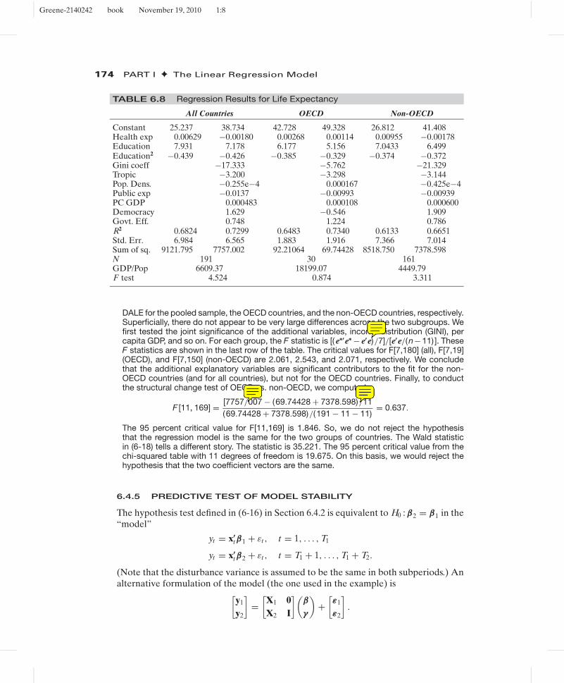
Example 6.10 The World Health ReportThe 2000 version of the World Health Organization’s (WHO) World Health Report contained amajor country-by-country inventory of the world’s health care systems. [World Health Organi-zation (2000). See also http://www.who.int/whr/en/.] The book documented years of researchand has thousands of pages of material. Among the most controversial and most publiclydebated parts of the report was a single chapter that described a comparison of the deliveryof health care by 191 countries—nearly all of the world’s population. [Evans et al. (2000a,b).See, e.g., Hilts (2000) for reporting in the popular press.] The study examined the efficiencyof health care delivery on two measures: the standard one that is widely studied, (disabilityadjusted) life expectancy (DALE), and an innovative new measure created by the authors thatwas a composite of five outcomes (COMP) and that accounted for efficiency and fairness indelivery. The regression-style modeling, which was done in the setting of a frontier model (seeChapter 18), related health care attainment to two major inputs, education and (per capita)health care expenditure. The residuals were analyzed to obtain the country comparisons.
The data in Appendix Table F6.3 were used by the researchers at the WHO for the study.(They used a panel of data for the years 1993 to 1997. We have extracted the 1997 data forthis example.) The WHO data have been used by many researchers in subsequent analyses.[See, e.g., Hollingsworth and Wildman (2002), Gravelle et al. (2002), and Greene (2004).]The regression model used by the WHO contained DALE or COMP on the left-hand sideand health care expenditure, education, and education squared on the right. Greene (2004)added a number of additional variables such as per capita GDP, a measure of the distributionof income, and World Bank measures of government effectiveness and democratization ofthe political structure.
Among the controversial aspects of the study was the fact that the model aggregatedcountries of vastly different characteristics. A second striking aspect of the results, suggestedin Hilts (2000) and documented in Greene (2004), was that, in fact, the “efficient” countries inthe study were the 30 relatively wealthy OECD members, while the rest of the world on averagefared much more poorly. We will pursue that aspect here with respect to DALE. Analysisof COMP is left as an exercise. Table 6.8 presents estimates of the regression models for
Greene-2140242 book November 19, 2010 1:8
174 PART I ✦ The Linear Regression Model
TABLE 6.8 Regression Results for Life Expectancy
All Countries OECD Non-OECD
Constant 25.237 38.734 42.728 49.328 26.812 41.408Health exp 0.00629 −0.00180 0.00268 0.00114 0.00955 −0.00178Education 7.931 7.178 6.177 5.156 7.0433 6.499Education2 −0.439 −0.426 −0.385 −0.329 −0.374 −0.372Gini coeff −17.333 −5.762 −21.329Tropic −3.200 −3.298 −3.144Pop. Dens. −0.255e−4 0.000167 −0.425e−4Public exp −0.0137 −0.00993 −0.00939PC GDP 0.000483 0.000108 0.000600Democracy 1.629 −0.546 1.909Govt. Eff. 0.748 1.224 0.786R2 0.6824 0.7299 0.6483 0.7340 0.6133 0.6651Std. Err. 6.984 6.565 1.883 1.916 7.366 7.014Sum of sq. 9121.795 7757.002 92.21064 69.74428 8518.750 7378.598N 191 30 161GDP/Pop 6609.37 18199.07 4449.79F test 4.524 0.874 3.311
DALE for the pooled sample, the OECD countries, and the non-OECD countries, respectively.Superficially, there do not appear to be very large differences across the two subgroups. Wefirst tested the joint significance of the additional variables, income distribution (GINI), percapita GDP, and so on. For each group, the F statistic is [( e∗′e∗ − e′e)/7]/[e′e/(n−11) ]. TheseF statistics are shown in the last row of the table. The critical values for F[7,180] (all), F[7,19](OECD), and F[7,150] (non-OECD) are 2.061, 2.543, and 2.071, respectively. We concludethat the additional explanatory variables are significant contributors to the fit for the non-OECD countries (and for all countries), but not for the OECD countries. Finally, to conductthe structural change test of OECD vs. non-OECD, we computed
F [11, 169] = [7757/007 − (69.74428 + 7378.598)/11(69.74428 + 7378.598)/(191 − 11 − 11)
= 0.637.
The 95 percent critical value for F[11,169] is 1.846. So, we do not reject the hypothesisthat the regression model is the same for the two groups of countries. The Wald statisticin (6-18) tells a different story. The statistic is 35.221. The 95 percent critical value from thechi-squared table with 11 degrees of freedom is 19.675. On this basis, we would reject thehypothesis that the two coefficient vectors are the same.
6.4.5 PREDICTIVE TEST OF MODEL STABILITY
The hypothesis test defined in (6-16) in Section 6.4.2 is equivalent to H0 : β2 = β1 in the“model”
yt = x′tβ1 + εt , t = 1, . . . , T1
yt = x′tβ2 + εt , t = T1 + 1, . . . , T1 + T2.
(Note that the disturbance variance is assumed to be the same in both subperiods.) Analternative formulation of the model (the one used in the example) is[
y1
y2
]=
[X1 0X2 I
](β
γ
)+
[ε1
ε2
].
Greene-2140242 book November 19, 2010 1:8
CHAPTER 6 ✦ Functional Form and Structural Change 175
This formulation states thatyt = x′
tβ1 + εt , t = 1, . . . , T1
yt = x′tβ2 + γt + εt , t = T1 + 1, . . . , T1 + T2.
Because each γt is unrestricted, this alternative formulation states that the regressionmodel of the first T1 periods ceases to operate in the second subperiod (and, in fact, nosystematic model operates in the second subperiod). A test of the hypothesis γ = 0 inthis framework would thus be a test of model stability. The least squares coefficients forthis regression can be found by using the formula for the partitioned inverse matrix(
bc
)=
[X′
1X1 + X′2X2 X′
2
X2 I
]−1 [X′
1y1 + X′2y2
y2
]
=[
(X′1X1)
−1 −(X′1X1)
−1X′2
−X2(X′1X1)
−1 I + X2(X′1X1)
−1X′2
] [X′
1y1 + X′2y2
y2
]
=(
b1
c2
)where b1 is the least squares slopes based on the first T1 observations and c2 is y2 −X2b1.The covariance matrix for the full set of estimates is s2 times the bracketed matrix. Thetwo subvectors of residuals in this regression are e1 = y1 − X1b1 and e2 = y2 − (X2b1 +Ic2) = 0, so the sum of squared residuals in this least squares regression is just e′
1e1.This is the same sum of squares as appears in (6-16). The degrees of freedom for thedenominator is [T1 + T2 − (K + T2)] = T1 − K as well, and the degrees of freedom forthe numerator is the number of elements in γ which is T2. The restricted regression withγ = 0 is the pooled model, which is likewise the same as appears in (6-16). This impliesthat the F statistic for testing the null hypothesis in this model is precisely that whichappeared earlier in (6-16), which suggests why the test is labeled the “predictive test.”
6.5 SUMMARY AND CONCLUSIONS
This chapter has discussed the functional form of the regression model. We examinedthe use of dummy variables and other transformations to build nonlinearity into themodel. We then considered other nonlinear models in which the parameters of thenonlinear model could be recovered from estimates obtained for a linear regression.The final sections of the chapter described hypothesis tests designed to reveal whetherthe assumed model had changed during the sample period, or was different for differentgroups of observations.
Key Terms and Concepts
• Binary variable• Chow test• Control group• Control observations• Difference in differences
• Dummy variable• Dummy variable trap• Exactly identified• Identification condition• Interaction terms
• Intrinsically linear• Knots• Loglinear model• Marginal effect• Natural experiment
Greene-2140242 book November 19, 2010 1:8
176 PART I ✦ The Linear Regression Model
• Nonlinear restriction• Overidentified• Piecewise continuous• Placebo effect• Predictive test
• Qualification indices• Response• Semilog equation• Spline• Structural change
• Threshold effects• Time profile• Treatment• Treatment group• Wald test
Exercises
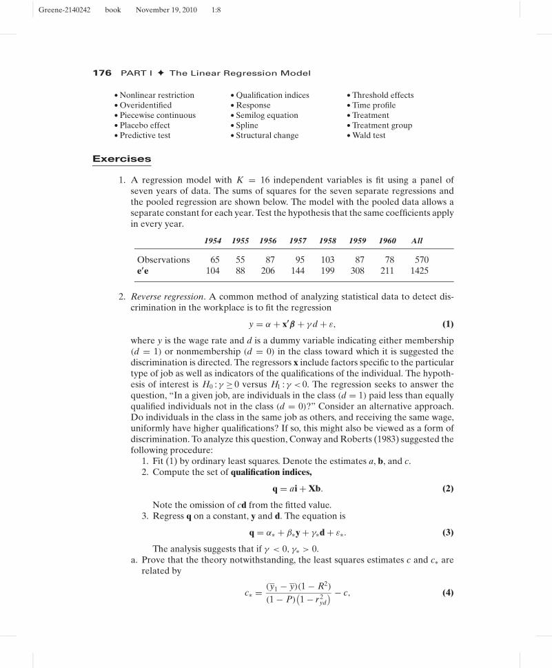
1. A regression model with K = 16 independent variables is fit using a panel ofseven years of data. The sums of squares for the seven separate regressions andthe pooled regression are shown below. The model with the pooled data allows aseparate constant for each year. Test the hypothesis that the same coefficients applyin every year.
1954 1955 1956 1957 1958 1959 1960 All
Observations 65 55 87 95 103 87 78 570e′e 104 88 206 144 199 308 211 1425
2. Reverse regression. A common method of analyzing statistical data to detect dis-crimination in the workplace is to fit the regression
y = α + x′β + γ d + ε, (1)
where y is the wage rate and d is a dummy variable indicating either membership(d = 1) or nonmembership (d = 0) in the class toward which it is suggested thediscrimination is directed. The regressors x include factors specific to the particulartype of job as well as indicators of the qualifications of the individual. The hypoth-esis of interest is H0 : γ ≥ 0 versus H1 : γ < 0. The regression seeks to answer thequestion, “In a given job, are individuals in the class (d = 1) paid less than equallyqualified individuals not in the class (d = 0)?” Consider an alternative approach.Do individuals in the class in the same job as others, and receiving the same wage,uniformly have higher qualifications? If so, this might also be viewed as a form ofdiscrimination. To analyze this question, Conway and Roberts (1983) suggested thefollowing procedure:
1. Fit (1) by ordinary least squares. Denote the estimates a, b, and c.2. Compute the set of qualification indices,
q = ai + Xb. (2)
Note the omission of cd from the fitted value.3. Regress q on a constant, y and d. The equation is
q = α∗ + β∗y + γ∗d + ε∗. (3)
The analysis suggests that if γ < 0, γ∗ > 0.a. Prove that the theory notwithstanding, the least squares estimates c and c∗ are
related by
c∗ = (y1 − y)(1 − R2)
(1 − P)(1 − r2
yd
) − c, (4)
Greene-2140242 book November 19, 2010 1:8
CHAPTER 6 ✦ Functional Form and Structural Change 177
wherey1 = mean of y for observations with d = 1,
y = mean of y for all observations,P = mean of d,
R2 = coefficient of determination for (1),
r2yd = squared correlation between y and d.
[Hint: The model contains a constant term. Thus, to simplify the algebra, assumethat all variables are measured as deviations from the overall sample means anduse a partitioned regression to compute the coefficients in (3). Second, in (2),use the result that based on the least squares results y = ai + Xb + cd + e, soq = y − cd − e. From here on, we drop the constant term. Thus, in the regressionin (3) you are regressing [y − cd − e] on y and d.
b. Will the sample evidence necessarily be consistent with the theory? [Hint: Sup-pose that c = 0.]
A symposium on the Conway and Roberts paper appeared in the Journal of Businessand Economic Statistics in April 1983.
3. Reverse regression continued. This and the next exercise continue the analysis ofExercise 2. In Exercise 2, interest centered on a particular dummy variable in whichthe regressors were accurately measured. Here we consider the case in which thecrucial regressor in the model is measured with error. The paper by Kamlich andPolachek (1982) is directed toward this issue.
Consider the simple errors in the variables model,
y = α + βx∗ + ε, x = x∗ + u,
where u and ε are uncorrelated and x is the erroneously measured, observed coun-terpart to x∗.a. Assume that x∗, u, and ε are all normally distributed with means μ∗, 0, and 0,
variances σ 2∗ , σ 2
u , and σ 2ε , and zero covariances. Obtain the probability limits of
the least squares estimators of α and β.b. As an alternative, consider regressing x on a constant and y, and then computing
the reciprocal of the estimate. Obtain the probability limit of this estimator.c. Do the “direct” and “reverse” estimators bound the true coefficient?
4. Reverse regression continued. Suppose that the model in Exercise 3 is extended toy = βx∗ +γ d +ε, x = x∗ +u. For convenience, we drop the constant term. Assumethat x∗, ε, and u are independent normally distributed with zero means. Supposethat d is a random variable that takes the values one and zero with probabilities π
and 1 − π in the population and is independent of all other variables in the model.To put this formulation in context, the preceding model (and variants of it) haveappeared in the literature on discrimination. We view y as a “wage” variable, x∗ as“qualifications,” and x as some imperfect measure such as education. The dummyvariable d is membership (d = 1) or nonmembership (d = 0) in some protected class.The hypothesis of discrimination turns on γ < 0 versus γ ≥ 0.a. What is the probability limit of c, the least squares estimator of γ , in the least
squares regression of y on x and d? [Hints: The independence of x∗ and d isimportant. Also, plim d′d/n = Var[d] + E2[d] = π(1 − π) + π2 = π . This minormodification does not affect the model substantively, but it greatly simplifies the

Greene-2140242 book November 19, 2010 1:8
178 PART I ✦ The Linear Regression Model
algebra.] Now suppose that x∗ and d are not independent. In particular, supposethat E [x∗ | d = 1] = μ1 and E [x∗ | d = 0] = μ0. Repeat the derivation with thisassumption.
b. Consider, instead, a regression of x on y and d. What is the probability limit ofthe coefficient on d in this regression? Assume that x∗ and d are independent.
c. Suppose that x∗ and d are not independent, but γ is, in fact, less than zero. As-suming that both preceding equations still hold, what is estimated by (y | d = 1)−(y | d = 0)? What does this quantity estimate if γ does equal zero?
Applications
1. In Application 1 in Chapter 3 and Application 1 in Chapter 5, we examined Koopand Tobias’s data on wages, education, ability, and so on. We continue the analysishere. (The source, location and configuration of the data are given in the earlierapplication.) We consider the model
ln Wage = β1 + β2 Educ + β3 Ability + β4 Experience
+ β5 Mother’s education + β6 Father’s education + β7 Broken home
+ β8 Siblings + ε.
a. Compute the full regression by least squares and report your results. Based onyour results, what is the estimate of the marginal value, in $/hour, of an additionalyear of education, for someone who has 12 years of education when all othervariables are at their means and Broken home = 0?
b. We are interested in possible nonlinearities in the effect of education on ln Wage.(Koop and Tobias focused on experience. As before, we are not attempting toreplicate their results.) A histogram of the education variable shows values from 9to 20, a huge spike at 12 years (high school graduation) and, perhaps surprisingly,a second at 15—intuition would have anticipated it at 16. Consider aggregatingthe education variable into a set of dummy variables:
HS = 1 if Educ ≤ 12, 0 otherwise
Col = 1 if Educ > 12 and Educ ≤ 16, 0 otherwise
Grad = 1 if Educ > 16, 0 otherwise.
Replace Educ in the model with (Col, Grad), making high school (HS) thebase category, and recompute the model. Report all results. How do the re-sults change? Based on your results, what is the marginal value of a collegedegree? (This is actually the marginal value of having 16 years of education—in recent years, college graduation has tended to require somewhat more thanfour years on average.) What is the marginal impact on ln Wage of a graduatedegree?
c. The aggregation in part b actually loses quite a bit of information. Another wayto introduce nonlinearity in education is through the function itself. Add Educ2
to the equation in part a and recompute the model. Again, report all results.What changes are suggested? Test the hypothesis that the quadratic term in the
Greene-2140242 book November 19, 2010 1:8
CHAPTER 6 ✦ Functional Form and Structural Change 179
equation is not needed—that is, that its coefficient is zero. Based on your results,sketch a profile of log wages as a function of education.
d. One might suspect that the value of education is enhanced by greater ability. Wecould examine this effect by introducing an interaction of the two variables inthe equation. Add the variable
Educ Ability = Educ × Ability
to the base model in part a. Now, what is the marginal value of an additionalyear of education? The sample mean value of ability is 0.052374. Compute aconfidence interval for the marginal impact on ln Wage of an additional year ofeducation for a person of average ability.
e. Combine the models in c and d. Add both Educ2 and Educ Ability to the basemodel in part a and reestimate. As before, report all results and describe yourfindings. If we define “low ability” as less than the mean and “high ability” asgreater than the mean, the sample averages are −0.798563 for the 7,864 low-ability individuals in the sample and +0.717891 for the 10,055 high-ability indi-viduals in the sample. Using the formulation in part c, with this new functionalform, sketch, describe, and compare the log wage profiles for low- and high-ability individuals.
2. (An extension of Application 1.) Here we consider whether different models asspecified in Application 1 would apply for individuals who reside in “Brokenhomes.” Using the results in Sections 6.4.1 and 6.4.4, test the hypothesis that thesame model (not including the Broken home dummy variable) applies to bothgroups of individuals, those with Broken home = 0 and with Broken home = 1.
3. In Solow’s classic (1957) study of technical change in the U.S. economy, he suggeststhe following aggregate production function: q(t) = A(t) f [k(t)], where q(t) is ag-gregate output per work hour, k(t) is the aggregate capital labor ratio, and A(t) isthe technology index. Solow considered four static models, q/A= α+β ln k, q/A=α − β/k, ln(q/A) = α + β ln k, and ln(q/A) = α + β/k. Solow’s data for the years1909 to 1949 are listed in Appendix Table F6.4.a. Use these data to estimate the α and β of the four functions listed above. (Note:
Your results will not quite match Solow’s. See the next exercise for resolution ofthe discrepancy.)
b. In the aforementioned study, Solow states:
A scatter of q/Aagainst k is shown in Chart 4. Considering the amountof a priori doctoring which the raw figures have undergone, the fit isremarkably tight. Except, that is, for the layer of points which are ob-viously too high. These maverick observations relate to the seven lastyears of the period, 1943–1949. From the way they lie almost exactlyparallel to the main scatter, one is tempted to conclude that in 1943 theaggregate production function simply shifted.
Compute a scatter diagram of q/Aagainst k and verify the result he notes above.c. Estimate the four models you estimated in the previous problem including a
dummy variable for the years 1943 to 1949. How do your results change? (Note:These results match those reported by Solow, although he did not report thecoefficient on the dummy variable.)
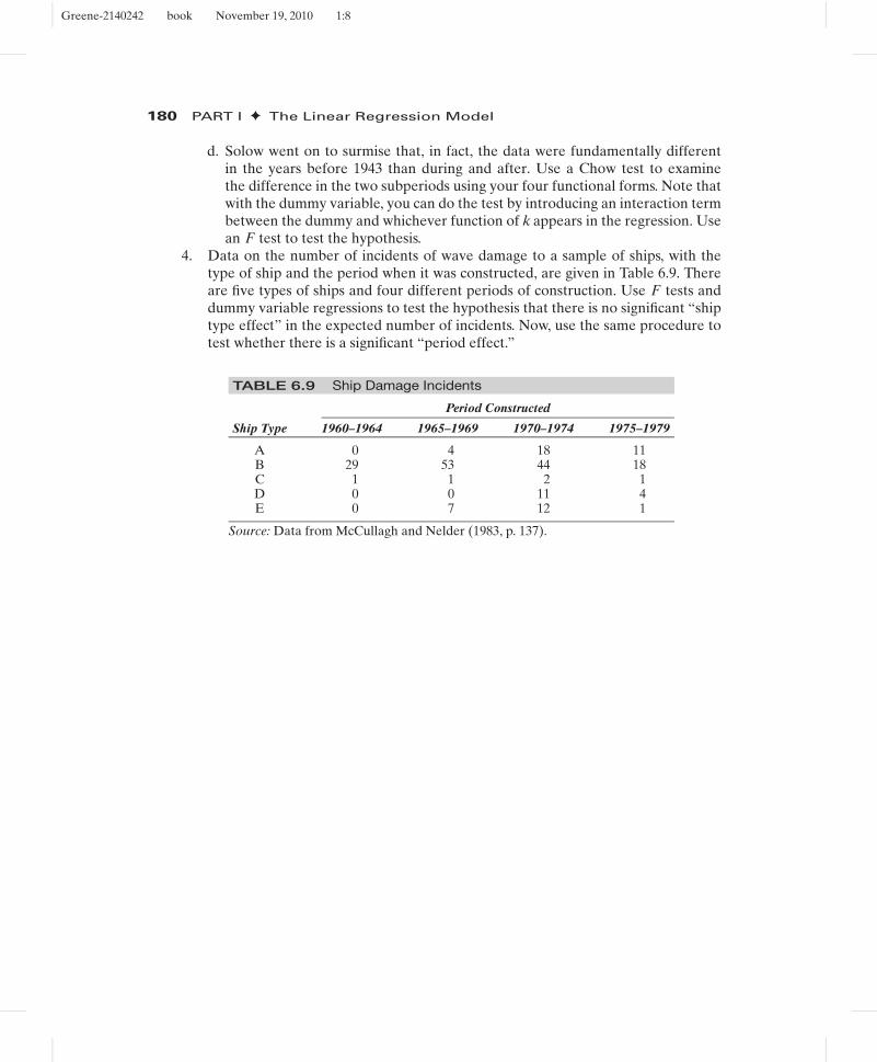
Greene-2140242 book November 19, 2010 1:8
180 PART I ✦ The Linear Regression Model
d. Solow went on to surmise that, in fact, the data were fundamentally differentin the years before 1943 than during and after. Use a Chow test to examinethe difference in the two subperiods using your four functional forms. Note thatwith the dummy variable, you can do the test by introducing an interaction termbetween the dummy and whichever function of k appears in the regression. Usean F test to test the hypothesis.
4. Data on the number of incidents of wave damage to a sample of ships, with thetype of ship and the period when it was constructed, are given in Table 6.9. Thereare five types of ships and four different periods of construction. Use F tests anddummy variable regressions to test the hypothesis that there is no significant “shiptype effect” in the expected number of incidents. Now, use the same procedure totest whether there is a significant “period effect.”
TABLE 6.9 Ship Damage Incidents
Period Constructed
Ship Type 1960–1964 1965–1969 1970–1974 1975–1979
A 0 4 18 11B 29 53 44 18C 1 1 2 1D 0 0 11 4E 0 7 12 1
Source: Data from McCullagh and Nelder (1983, p. 137).