forecasting to accompany russell and taylor, operations management, 4th edition, 2003...
Post on 21-Dec-2015
253 views
TRANSCRIPT

ForecastingForecasting
To Accompany Russell and Taylor, Operations Management, 4th Edition, 2003 Prentice-Hall, Inc. All rights reserved.
ForecastingForecasting
Predicting future eventsPredicting future eventsUsually demand behavior Usually demand behavior
over a time frameover a time frame

Forecast:• A statement about the future value of a variable of
interest such as demand.• Forecasts affect decisions and activities throughout
an organization–Accounting, finance–Human resources–Marketing–MIS–Operations–Product / service design
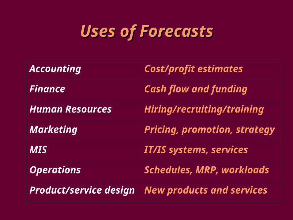
Accounting Cost/profit estimates
Finance Cash flow and funding
Human Resources Hiring/recruiting/training
Marketing Pricing, promotion, strategy
MIS IT/IS systems, services
Operations Schedules, MRP, workloads
Product/service design New products and services
Uses of ForecastsUses of Forecasts

Uses of ForecastsUses of Forecasts
To help managers plan the systemTo help managers plan the use of the
system.
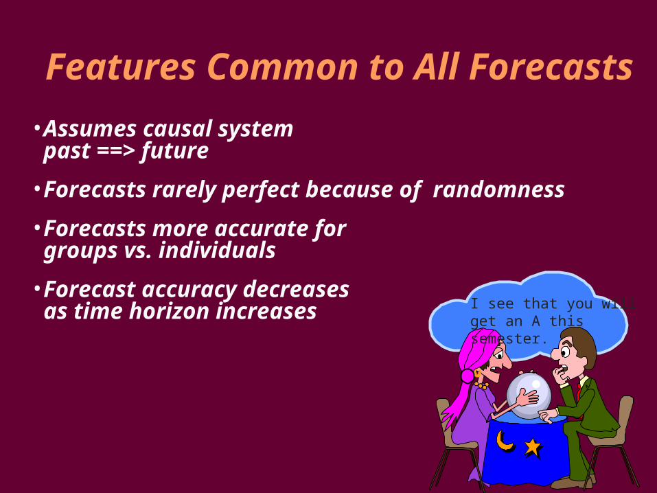
• Assumes causal systempast ==> future
• Forecasts rarely perfect because of randomness
• Forecasts more accurate forgroups vs. individuals
• Forecast accuracy decreases as time horizon increases I see that you will
get an A this semester.
Features Common to All Forecasts

Elements of a Good ForecastElements of a Good Forecast
Timely
AccurateReliable
Mea
ningfu
lWritten
Easy
to u
se
Time FrameTime Frame in Forecasting in Forecasting
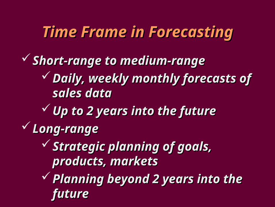
Short-range to medium-rangeShort-range to medium-rangeDaily, weekly monthly forecasts of Daily, weekly monthly forecasts of
sales datasales dataUp to 2 years into the futureUp to 2 years into the future
Long-rangeLong-rangeStrategic planning of goals, Strategic planning of goals,
products, marketsproducts, marketsPlanning beyond 2 years into the Planning beyond 2 years into the
futurefuture
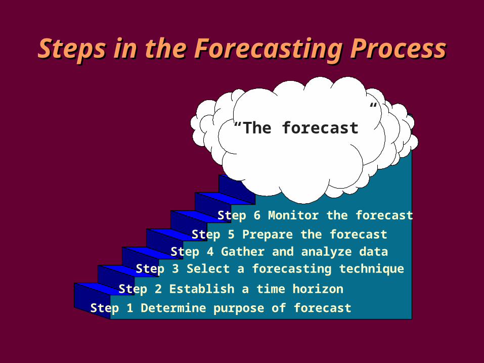
Steps in the Forecasting ProcessSteps in the Forecasting Process
Step 1 Determine purpose of forecast
Step 2 Establish a time horizon
Step 3 Select a forecasting technique
Step 4 Gather and analyze data
Step 5 Prepare the forecast
Step 6 Monitor the forecast
“The forecast”

Forecasting ProcessForecasting Process
6. Check forecast accuracy with one or more measures
4. Select a forecast model that seems appropriate for data
5. Develop/compute forecast for period of historical data
8a. Forecast over planning horizon
9. Adjust forecast based on additional qualitative information and insight
10. Monitor results and measure forecast accuracy
8b. Select new forecast model or adjust parameters of existing model
7.Is accuracy of forecast
acceptable?
1. Identify the purpose of forecast
3. Plot data and identify patterns
2. Collect historical data
Approaches to ForecastingApproaches to Forecasting
• Qualitative methodsQualitative methods– Based on subjective methodsBased on subjective methods
• Quantitative methodsQuantitative methods– Based on mathematical formulasBased on mathematical formulas
Approaches to ForecastingApproaches to Forecasting• Judgmental (Qualitative)- uses
subjective inputs
• Time series - uses historical data assuming the future will be like the past
• Associative models - uses explanatory variables to predict the future

Judgmental ForecastsJudgmental Forecasts• Executive opinions
• Sales force opinions
• Consumer surveys
• Outside opinion
• Delphi method– Opinions of managers and staff
– Achieves a consensus forecast
Time SeriesTime Series
A time series is a time-ordered sequence of observations taken at regular intervals (eg. Hourly, daily, weekly, monthly, quarterly, annually)
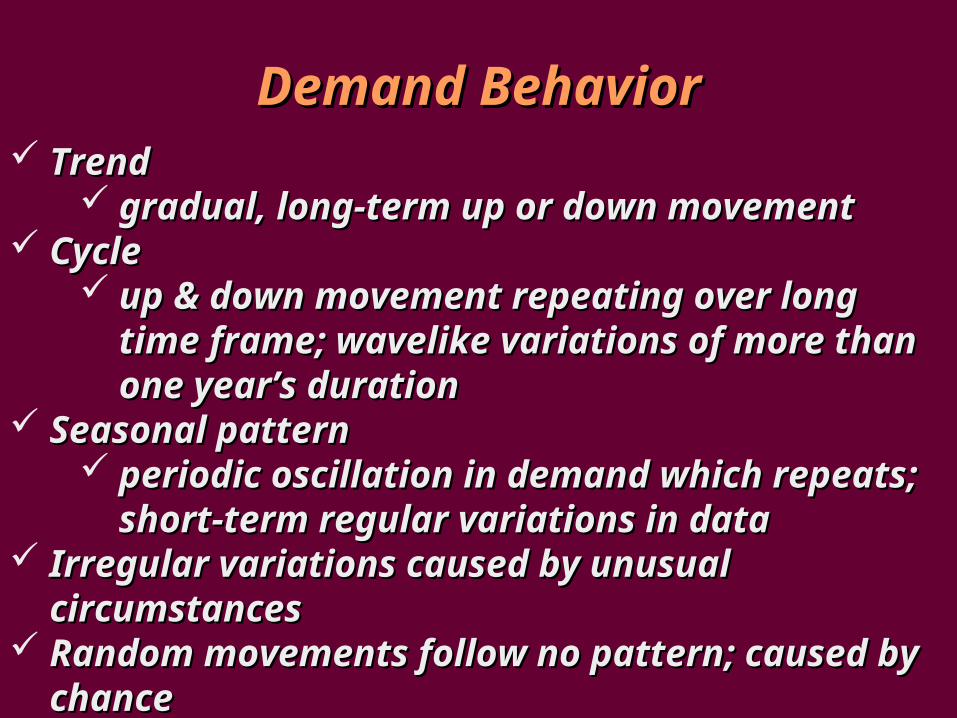
Demand BehaviorDemand Behavior TrendTrend
gradual, long-term up or down movementgradual, long-term up or down movement CycleCycle
up & down movement repeating over long time up & down movement repeating over long time frameframe; wavelike variations of more than one ; wavelike variations of more than one year’s durationyear’s duration
Seasonal patternSeasonal pattern periodic oscillation in demand which repeatsperiodic oscillation in demand which repeats; ;
short-term regular variations in datashort-term regular variations in data Irregular variations caused by unusual Irregular variations caused by unusual
circumstancescircumstances Random movements follow no patternRandom movements follow no pattern; caused by ; caused by
chancechance

Forms of Forecast MovementForms of Forecast Movement
TimeTime(a) Trend(a) Trend
TimeTime(d) Trend with seasonal pattern(d) Trend with seasonal pattern
TimeTime(c) Seasonal pattern(c) Seasonal pattern
TimeTime(b) Cycle(b) Cycle
Dem
and
Dem
and
Dem
and
Dem
and
Dem
and
Dem
and
Dem
and
Dem
and
Random Random movementmovement
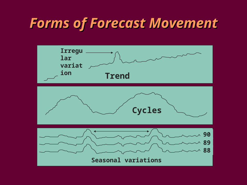
Trend
Irregularvariation
Seasonal variations
908988
Cycles
Forms of Forecast MovementForms of Forecast Movement

Time Series MethodsTime Series Methods
Naive forecastsNaive forecasts Forecast = data from past periodForecast = data from past periodStatistical methods using historical Statistical methods using historical
datadata Moving averageMoving average Exponential smoothingExponential smoothing Linear trend lineLinear trend line
Assume patterns will Assume patterns will repeatrepeat
Demand?

Naive ForecastsNaive Forecasts
Uh, give me a minute.... We sold 250 wheels lastweek.... Now, next week we should sell....
The forecast for any period equals the previous period’s actual value.

• Simple to use
• Virtually no cost
• Quick and easy to prepare
• Data analysis is nonexistent
• Easily understandable
• Cannot provide high accuracy
• Can be a standard for accuracy
Naïve ForecastsNaïve Forecasts
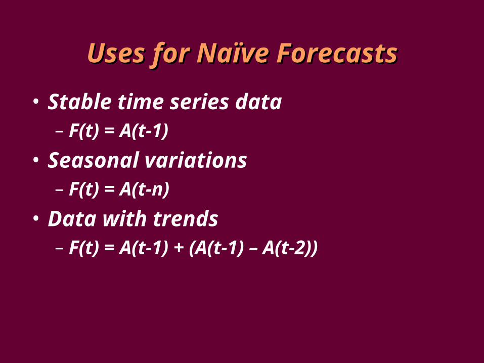
• Stable time series data– F(t) = A(t-1)
• Seasonal variations– F(t) = A(t-n)
• Data with trends– F(t) = A(t-1) + (A(t-1) – A(t-2))
Uses for Naïve ForecastsUses for Naïve Forecasts
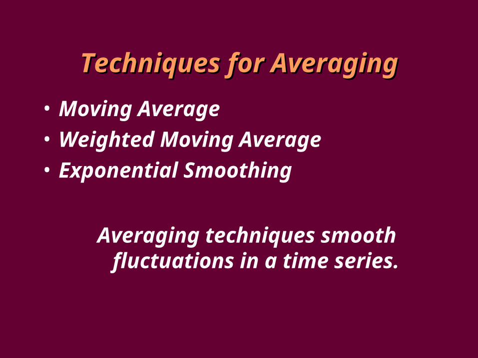
Techniques for AveragingTechniques for Averaging
• Moving Average
• Weighted Moving Average
• Exponential Smoothing
Averaging techniques smooth fluctuations in a time series.
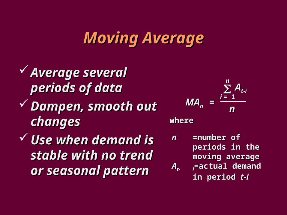
Moving AverageMoving Average
MAMAnn = =
nn
ii = 1= 1 AAt-it-i
nnwherewhere
nn ==number of periods number of periods in the moving in the moving averageaverage
AAt-t- ii==actual actual demand in demand in
period period t-t-ii
Average several Average several periods of dataperiods of data
Dampen, smooth out Dampen, smooth out changeschanges
Use when demand is Use when demand is stable with no trend stable with no trend or seasonal patternor seasonal pattern

Moving AveragesMoving Averages• Moving average – A technique that
averages a number of recent actual values, updated as new values become available.
Ft = MAn= n
At-n + … At-2 + At-1
Ft = Forecast for time period t
MAn= n period moving average
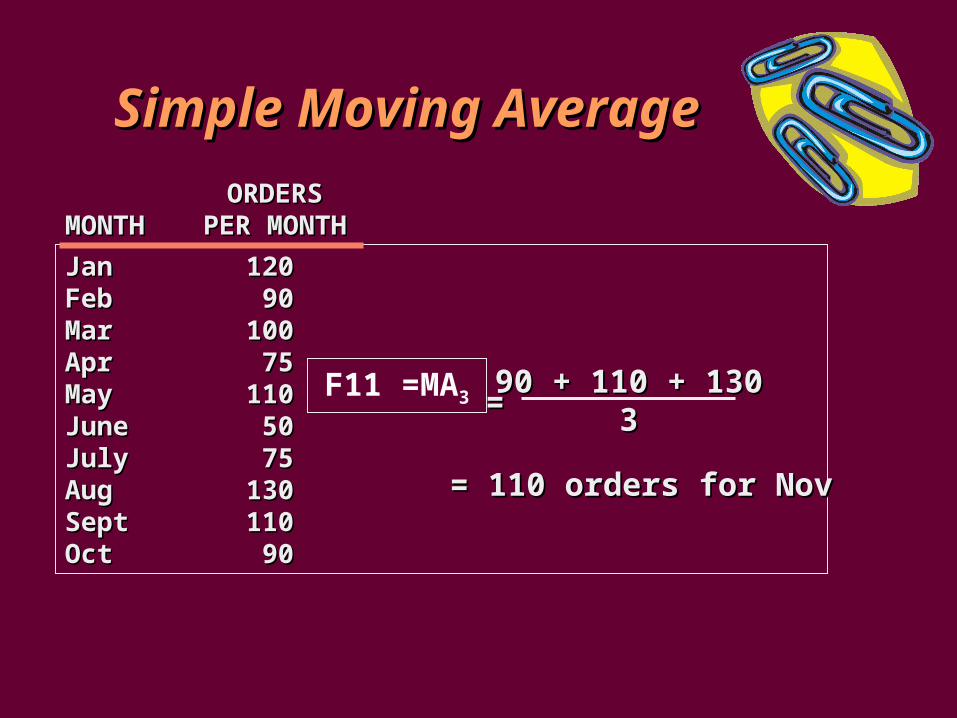
JanJan 120120FebFeb 9090MarMar 100100AprApr 7575MayMay 110110JuneJune 5050JulyJuly 7575AugAug 130130SeptSept 110110OctOct 9090
ORDERSORDERSMONTHMONTH PER MONTHPER MONTH
==90 + 110 + 13090 + 110 + 130
33
= 110 orders for Nov= 110 orders for Nov
Simple Moving AverageSimple Moving Average
F11 =MA3
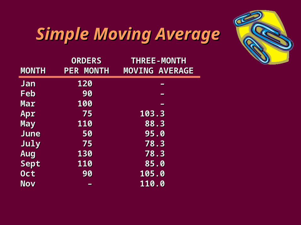
JanJan 120120 ––FebFeb 9090 – –MarMar 100100 – –AprApr 7575 103.3103.3MayMay 110110 88.388.3JuneJune 5050 95.095.0JulyJuly 7575 78.378.3AugAug 130130 78.378.3SeptSept 110110 85.085.0OctOct 9090 105.0105.0NovNov – – 110.0110.0
ORDERSORDERS THREE-MONTHTHREE-MONTHMONTHMONTH PER MONTHPER MONTH MOVING AVERAGEMOVING AVERAGE
Simple Moving AverageSimple Moving Average

JanJan 120120 ––FebFeb 9090 – –MarMar 100100 – –AprApr 7575 103.3103.3MayMay 110110 88.388.3JuneJune 5050 95.095.0JulyJuly 7575 78.378.3AugAug 130130 78.378.3SeptSept 110110 85.085.0OctOct 9090 105.0105.0NovNov – – 110.0110.0
ORDERSORDERS THREE-MONTHTHREE-MONTHMONTHMONTH PER MONTHPER MONTH MOVING AVERAGEMOVING AVERAGE
90 + 110 + 130 + 75 + 5090 + 110 + 130 + 75 + 5055
= 91 orders for Nov= 91 orders for Nov
Simple Moving AverageSimple Moving Average
F11 MA5 =

Simple Moving AverageSimple Moving Average
JanJan 120120 –– – –FebFeb 9090 – – – –MarMar 100100 – – – –AprApr 7575 103.3103.3 – –MayMay 110110 88.388.3 – –JuneJune 5050 95.095.0 99.099.0JulyJuly 7575 78.378.3 85.085.0AugAug 130130 78.378.3 82.082.0SeptSept 110110 85.085.0 88.088.0OctOct 9090 105.0105.0 95.095.0NovNov – – 110.0110.0 91.091.0
ORDERSORDERS THREE-MONTHTHREE-MONTH FIVE-MONTHFIVE-MONTHMONTHMONTH PER MONTHPER MONTH MOVING AVERAGEMOVING AVERAGE MOVING AVERAGEMOVING AVERAGE
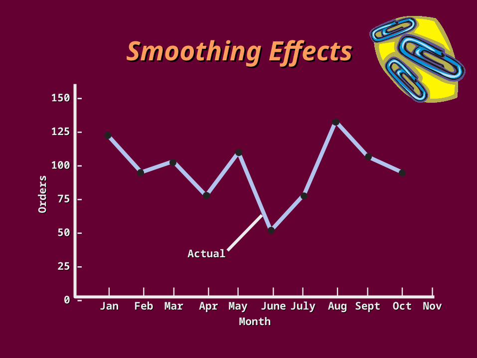
Smoothing EffectsSmoothing Effects
150 150 –
125 125 –
100 100 –
75 75 –
50 50 –
25 25 –
0 0 –| | | | | | | | | | |
JanJan FebFeb MarMar AprApr MayMay JuneJune JulyJuly AugAug SeptSept OctOct NovNov
Ord
ers
Ord
ers
MonthMonth
ActualActual

Smoothing EffectsSmoothing Effects
150 150 –
125 125 –
100 100 –
75 75 –
50 50 –
25 25 –
0 0 –| | | | | | | | | | |
JanJan FebFeb MarMar AprApr MayMay JuneJune JulyJuly AugAug SeptSept OctOct NovNov
3-month3-month
ActualActual
Ord
ers
Ord
ers
MonthMonth
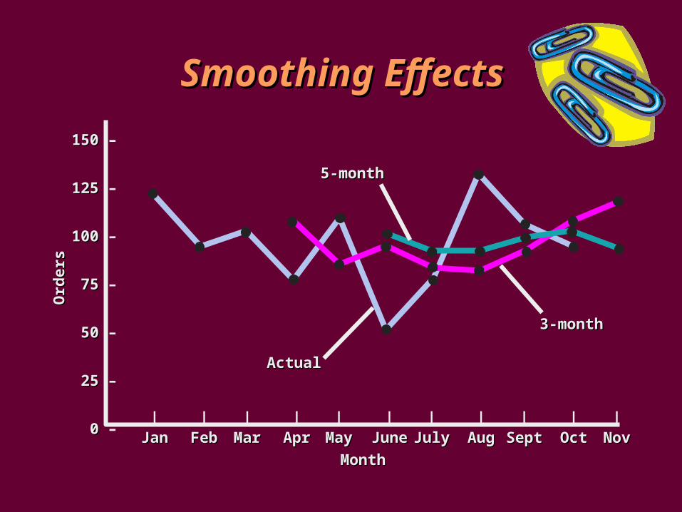
Smoothing EffectsSmoothing Effects
150 150 –
125 125 –
100 100 –
75 75 –
50 50 –
25 25 –
0 0 –| | | | | | | | | | |
JanJan FebFeb MarMar AprApr MayMay JuneJune JulyJuly AugAug SeptSept OctOct NovNov
5-month5-month
3-month3-month
ActualActual
Ord
ers
Ord
ers
MonthMonth
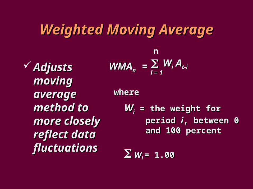
Weighted Moving AverageWeighted Moving Average
WMAWMAnn = = ii = 1 = 1 WWii AAt-it-i
wherewhere
WWii = the weight for period = the weight for period ii, ,
between 0 and 100 between 0 and 100 percentpercent
WWii = 1.00= 1.00
Adjusts Adjusts moving moving average average method to method to more closely more closely reflect data reflect data fluctuationsfluctuations
n
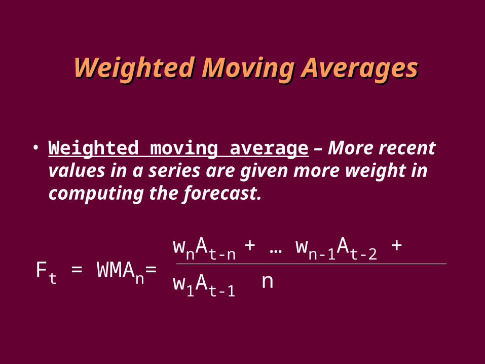
Weighted Weighted Moving AveragesMoving Averages
• Weighted moving average – More recent values in a series are given more weight in computing the forecast.
Ft = WMAn= n
wnAt-n + … wn-1At-2 + w1At-1
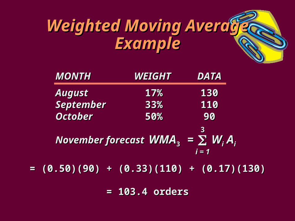
Weighted Moving Average Weighted Moving Average ExampleExample
MONTH MONTH WEIGHT WEIGHT DATADATA
AugustAugust 17%17% 130130SeptemberSeptember 33%33% 110110OctoberOctober 50%50% 9090
November forecastNovember forecast WMAWMA33 = = 33
ii = 1 = 1 WWii AAii
= (0.50)(90) + (0.33)(110) + (0.17)(130)= (0.50)(90) + (0.33)(110) + (0.17)(130)
= 103.4 orders= 103.4 orders
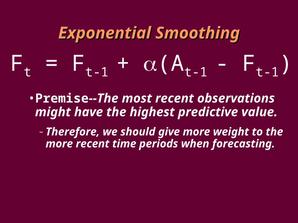
Exponential SmoothingExponential Smoothing
• Premise--The most recent observations might have the highest predictive value.
– Therefore, we should give more weight to the more recent time periods when forecasting.
Ft = Ft-1 + (At-1 - Ft-1)

Exponential SmoothingExponential Smoothing
• Weighted averaging method based on previous forecast plus a percentage of the forecast error
• A-F is the error term, is the % feedback or a percentage of forecast error
Ft = Ft-1 + (At-1 - Ft-1)
FtFt =forecast for =forecast for the the next periodnext period AAtt -1-1 =actual demand for =actual demand for the the present periodpresent period
FtFt -1 -1 ==previously determined forecast for previously determined forecast for the the present periodpresent periodαα == weighting factor, smoothing constantweighting factor, smoothing constant
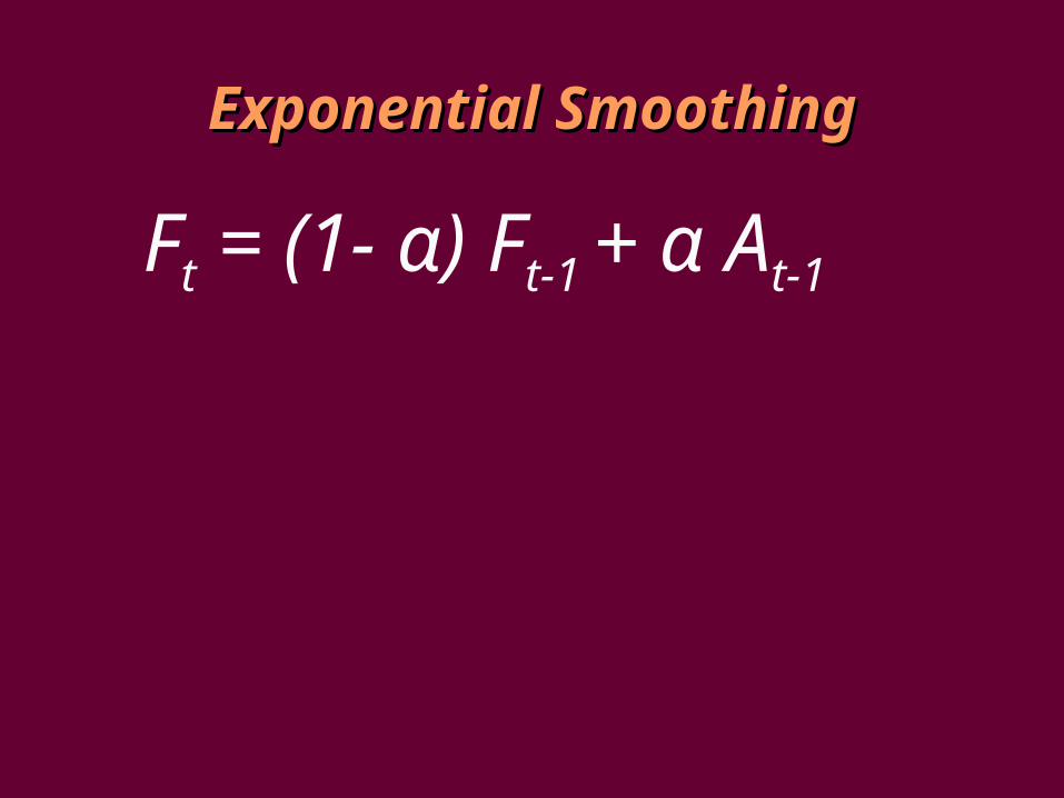
Exponential SmoothingExponential Smoothing
Ft = (1- α) Ft-1 + α At-1
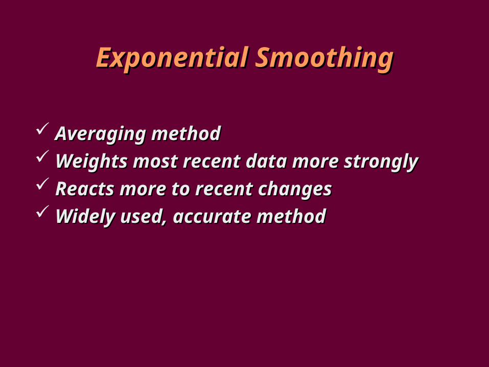
Averaging method Averaging method Weights most recent data more stronglyWeights most recent data more strongly Reacts more to recent changesReacts more to recent changes Widely used, accurate methodWidely used, accurate method
Exponential SmoothingExponential Smoothing

Effect of Smoothing ConstantEffect of Smoothing Constant
0.0 0.0 1.0 1.0
If If = 0.20, then = 0.20, then FFt t +1 +1 = 0.20= 0.20AAtt + 0.80 + 0.80 FFtt
If If = 0, then = 0, then FFtt +1 +1 = 0= 0AAtt + 1 + 1 FFtt 0 = 0 = FFtt
Forecast does not reflect recent dataForecast does not reflect recent data
If If = 1, then = 1, then FFt t +1 +1 = 1= 1AAtt + 0 + 0 FFtt ==AAtt Forecast based only on most recent dataForecast based only on most recent data
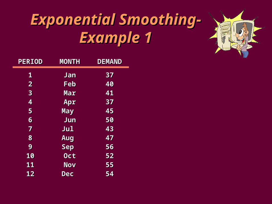
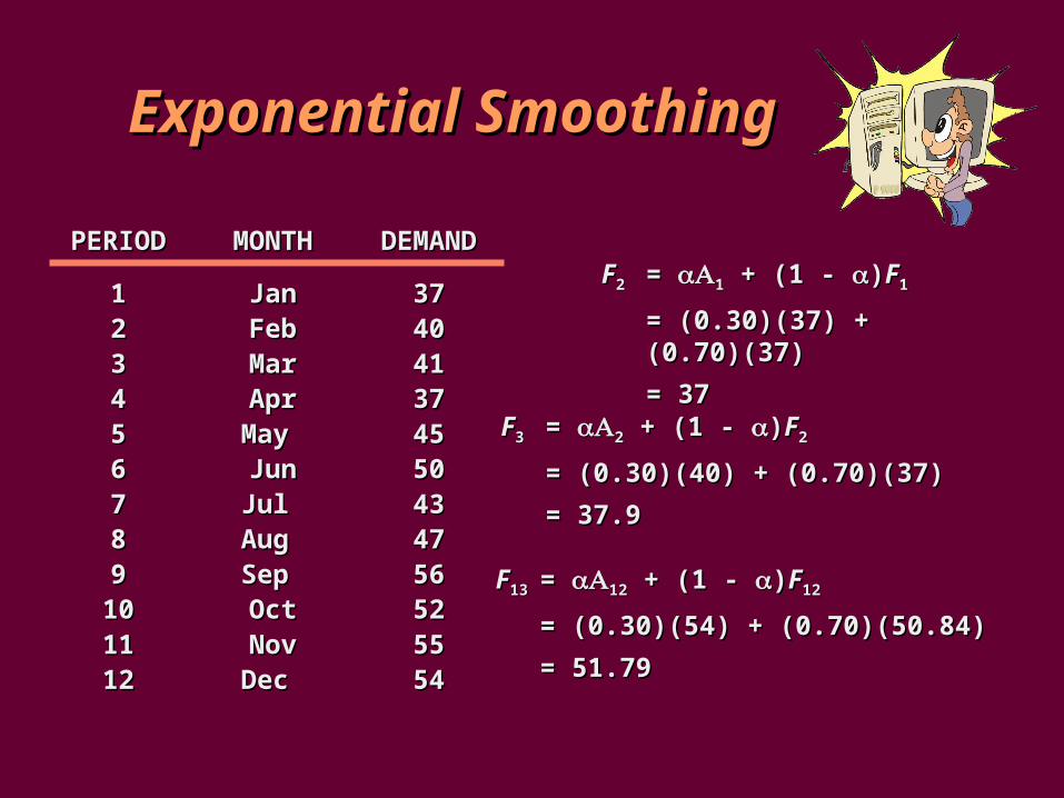
PERIODPERIOD MONTHMONTH DEMANDDEMAND
11 JanJan 373722 FebFeb 404033 MarMar 414144 AprApr 373755 May May 454566 JunJun 505077 Jul Jul 434388 Aug Aug 474799 Sep Sep 5656
1010 OctOct 52521111 NovNov 55551212 Dec Dec 5454
Exponential SmoothingExponential Smoothing--Example 1Example 1
PERIODPERIOD MONTHMONTH DEMANDDEMAND
11 JanJan 373722 FebFeb 404033 MarMar 414144 AprApr 373755 May May 454566 JunJun 505077 Jul Jul 434388 Aug Aug 474799 Sep Sep 5656
1010 OctOct 52521111 NovNov 55551212 Dec Dec 5454
FF22 = = 11 + (1 - + (1 - ))FF11
= (0.30)(37) + (0.70)(37)= (0.30)(37) + (0.70)(37)
= 37= 37
FF33 = = 22 + (1 - + (1 - ))FF22
= (0.30)(40) + (0.70)(37)= (0.30)(40) + (0.70)(37)
= 37.9= 37.9
FF1313 = = 1212 + (1 - + (1 - ))FF1212
= (0.30)(54) + (0.70)(50.84)= (0.30)(54) + (0.70)(50.84)
= 51.79= 51.79
Exponential SmoothingExponential Smoothing
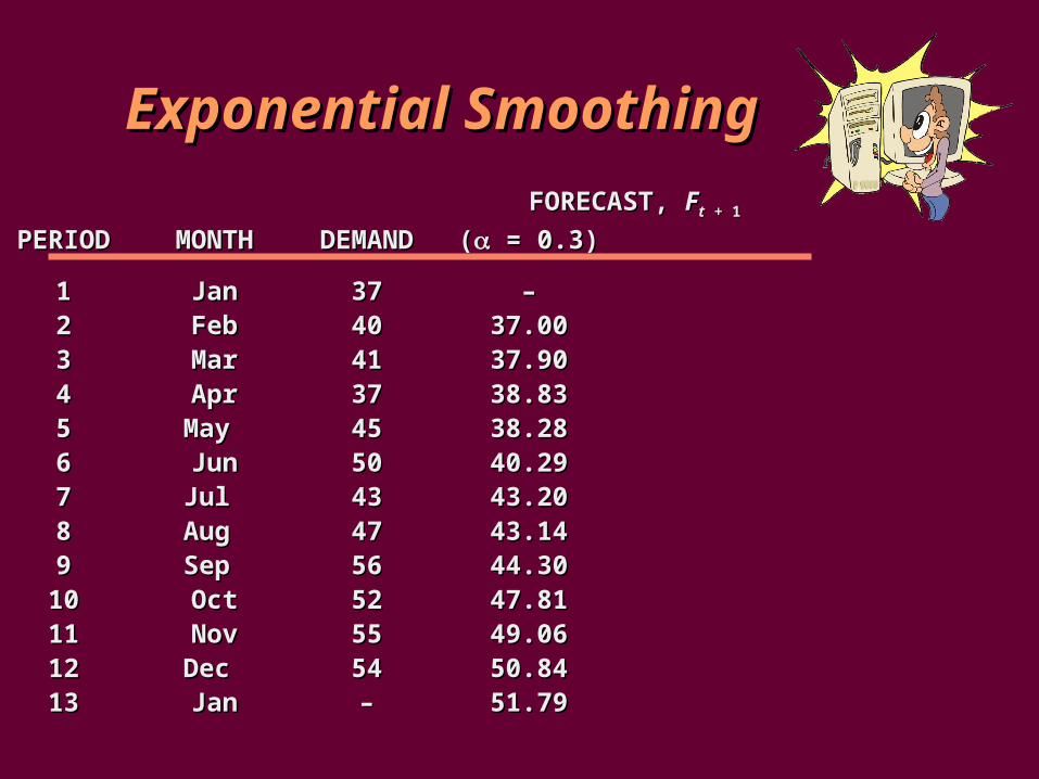
FORECAST, FORECAST, FFtt + 1 + 1
PERIODPERIOD MONTHMONTH DEMANDDEMAND (( = 0.3) = 0.3)
11 JanJan 3737 ––22 FebFeb 4040 37.0037.0033 MarMar 4141 37.9037.9044 AprApr 3737 38.8338.8355 May May 4545 38.2838.2866 JunJun 5050 40.2940.2977 Jul Jul 4343 43.2043.2088 Aug Aug 4747 43.1443.1499 Sep Sep 5656 44.3044.30
1010 OctOct 5252 47.8147.811111 NovNov 5555 49.0649.061212 Dec Dec 5454 50.8450.841313 JanJan –– 51.7951.79
Exponential SmoothingExponential Smoothing

FORECAST, FORECAST, FFtt + 1 + 1
PERIODPERIOD MONTHMONTH DEMANDDEMAND (( = 0.3) = 0.3) (( = 0.5) = 0.5)
11 JanJan 3737 –– ––22 FebFeb 4040 37.0037.00 37.0037.0033 MarMar 4141 37.9037.90 38.5038.5044 AprApr 3737 38.8338.83 39.7539.7555 May May 4545 38.2838.28 38.3738.3766 JunJun 5050 40.2940.29 41.6841.6877 Jul Jul 4343 43.2043.20 45.8445.8488 Aug Aug 4747 43.1443.14 44.4244.4299 Sep Sep 5656 44.3044.30 45.7145.71
1010 OctOct 5252 47.8147.81 50.8550.851111 NovNov 5555 49.0649.06 51.4251.421212 Dec Dec 5454 50.8450.84 53.2153.211313 JanJan –– 51.7951.79 53.6153.61
Exponential SmoothingExponential Smoothing

70 70 –
60 60 –
50 50 –
40 40 –
30 30 –
20 20 –
1010 –
0 0 –| | | | | | | | | | | | |11 22 33 44 55 66 77 88 99 1010 1111 1212 1313
ActualActual
Ord
ers
Ord
ers
MonthMonth
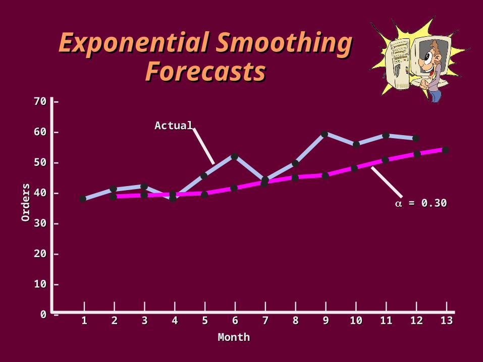
Exponential Smoothing Exponential Smoothing ForecastsForecasts
70 70 –
60 60 –
50 50 –
40 40 –
30 30 –
20 20 –
1010 –
0 0 –| | | | | | | | | | | | |11 22 33 44 55 66 77 88 99 1010 1111 1212 1313
ActualActual
Ord
ers
Ord
ers
MonthMonth
= 0.30= 0.30
Exponential Smoothing Exponential Smoothing ForecastsForecasts

70 70 –
60 60 –
50 50 –
40 40 –
30 30 –
20 20 –
1010 –
0 0 –| | | | | | | | | | | | |11 22 33 44 55 66 77 88 99 1010 1111 1212 1313
= 0.50= 0.50ActualActual
Ord
ers
Ord
ers
MonthMonth
= 0.30= 0.30
Exponential Smoothing Exponential Smoothing ForecastsForecasts
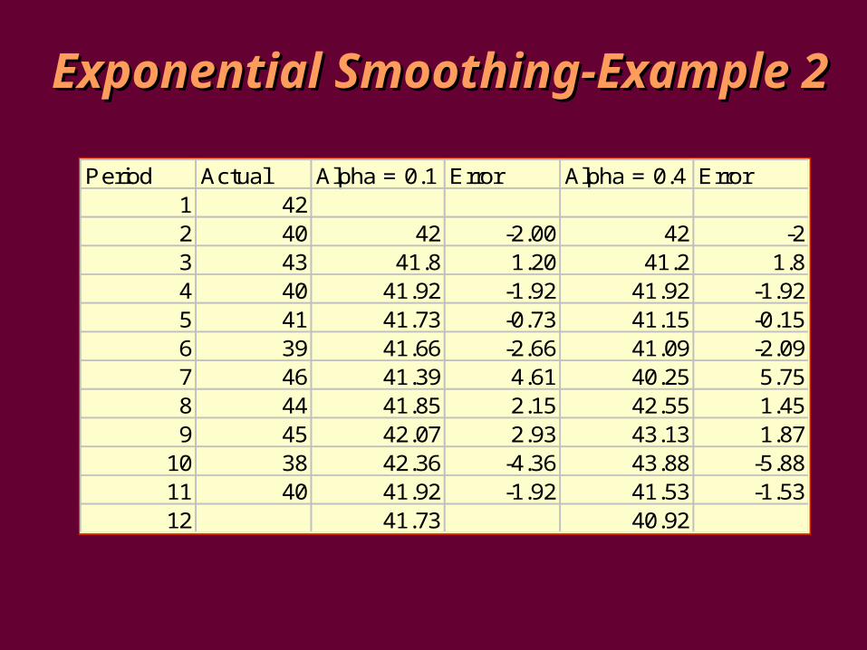
Period Actual Alpha = 0.1 Error Alpha = 0.4 Error1 422 40 42 -2.00 42 -23 43 41.8 1.20 41.2 1.84 40 41.92 -1.92 41.92 -1.925 41 41.73 -0.73 41.15 -0.156 39 41.66 -2.66 41.09 -2.097 46 41.39 4.61 40.25 5.758 44 41.85 2.15 42.55 1.459 45 42.07 2.93 43.13 1.87
10 38 42.36 -4.36 43.88 -5.8811 40 41.92 -1.92 41.53 -1.5312 41.73 40.92
Exponential SmoothingExponential Smoothing--Example 2Example 2
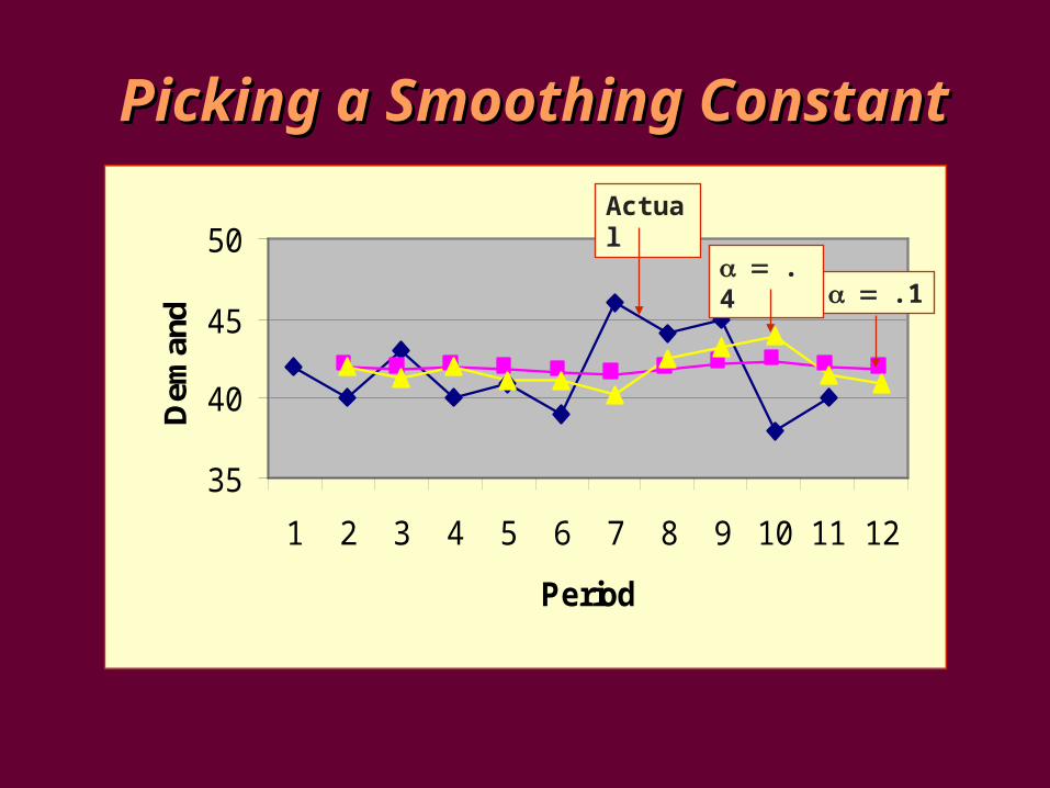
Picking a Smoothing ConstantPicking a Smoothing Constant
35
40
45
50
1 2 3 4 5 6 7 8 9 10 11 12
Period
Dem
and .1
.4
Actual
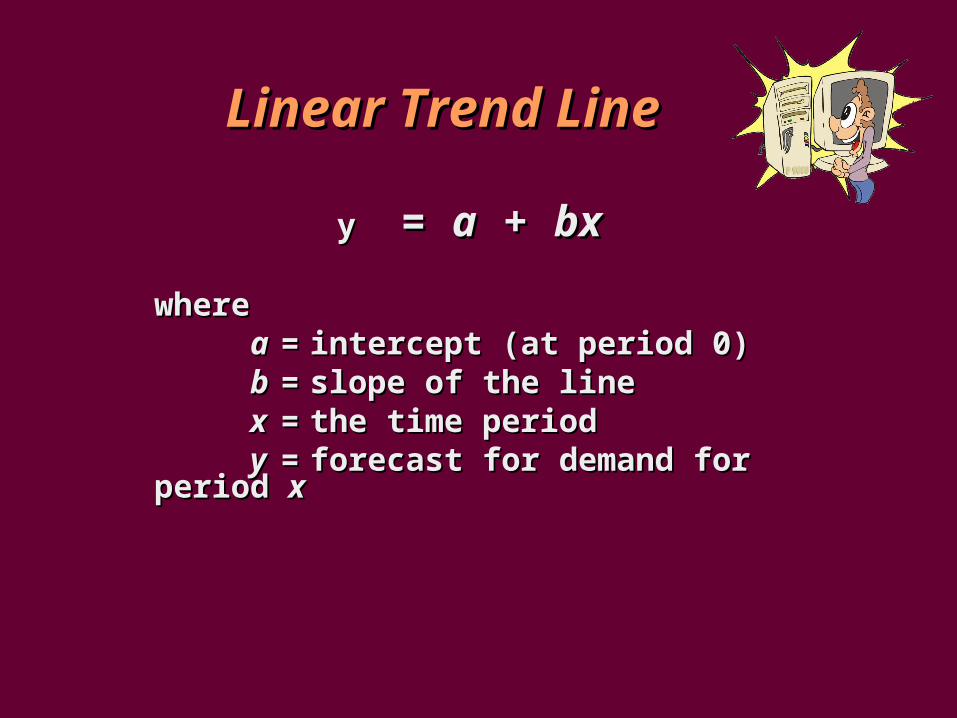
yy = = aa + + bxbx
wherewhereaa == intercept (at period 0)intercept (at period 0)bb == slope of the lineslope of the linexx == the time periodthe time periodyy == forecast for demand for period forecast for demand for period xx
Linear Trend LineLinear Trend Line
yy = = aa + + bxbx
wherewhereaa == intercept (at period 0)intercept (at period 0)bb == slope of the lineslope of the linexx == the time periodthe time periodyy == forecast for demand for period forecast for demand for period xx
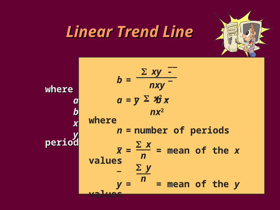
b =
a = y - b x
wheren = number of periods
x = = mean of the x values
y = = mean of the y values
xy -
nxy
x2 - nx2
xn
yn
Linear Trend LineLinear Trend Line
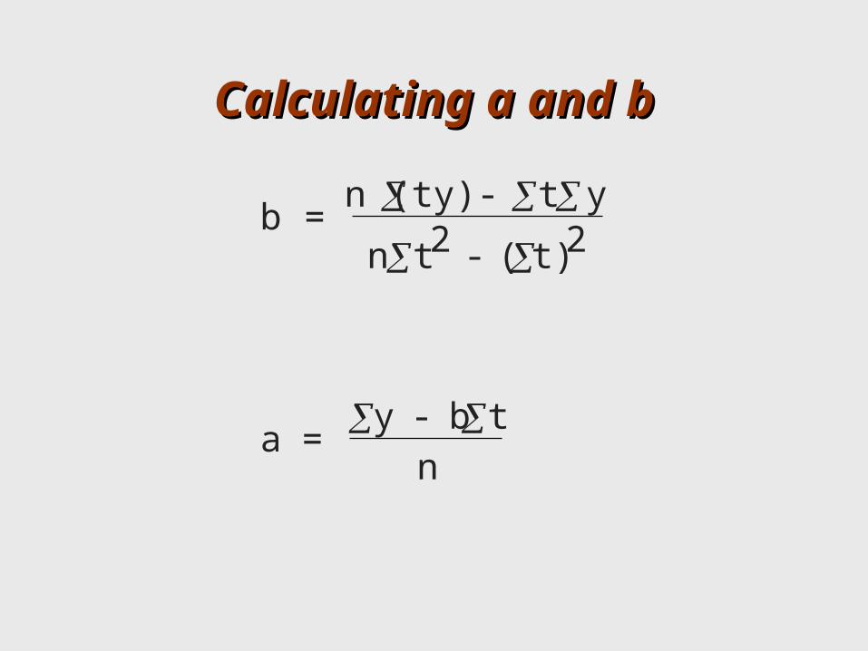
Calculating a and bCalculating a and b
b = n (ty) - t y
n t2 - ( t)2
a = y - b t
n
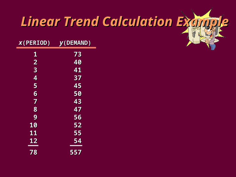
xx(PERIOD)(PERIOD) yy(DEMAND)(DEMAND)
11 737322 404033 414144 373755 454566 505077 434388 474799 5656
1010 52521111 55551212 5454
7878 557557
LLinear Trend Calculationinear Trend Calculation Example Example
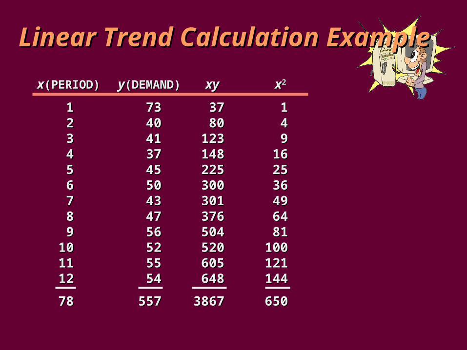
xx(PERIOD)(PERIOD) yy(DEMAND)(DEMAND) xyxy xx22
11 7373 3737 1122 4040 8080 4433 4141 123123 9944 3737 148148 161655 4545 225225 252566 5050 300300 363677 4343 301301 494988 4747 376376 646499 5656 504504 8181
1010 5252 520520 1001001111 5555 605605 1211211212 5454 648648 144144
7878 557557 38673867 650650
LLinear Trend Calculationinear Trend Calculation Example Example
LLinear Trend Calculationinear Trend Calculation Example Example
xx(PERIOD)(PERIOD) yy(DEMAND)(DEMAND) xyxy xx22
11 7373 3737 1122 4040 8080 4433 4141 123123 9944 3737 148148 161655 4545 225225 252566 5050 300300 363677 4343 301301 494988 4747 376376 646499 5656 504504 8181
1010 5252 520520 1001001111 5555 605605 1211211212 5454 648648 144144
7878 557557 38673867 650650
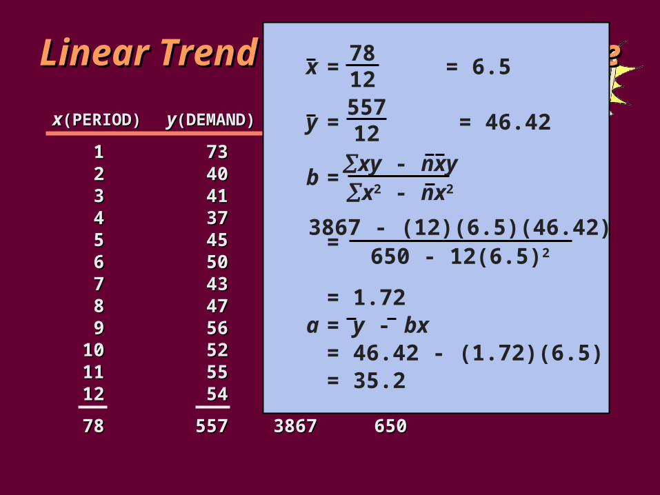
x = = 6.5
y = = 46.42
b =
=
= 1.72a = y - bx
= 46.42 - (1.72)(6.5)= 35.2
3867 - (12)(6.5)(46.42)650 - 12(6.5)2
xy - nxyx2 - nx2
781255712

Linear Trend CalculationLinear Trend Calculation Example Example
xx(PERIOD)(PERIOD) yy(DEMAND)(DEMAND) xyxy xx22
11 7373 3737 1122 4040 8080 4433 4141 123123 9944 3737 148148 161655 4545 225225 252566 5050 300300 363677 4343 301301 494988 4747 376376 646499 5656 504504 8181
1010 5252 520520 1001001111 5555 605605 1211211212 5454 648648 144144
7878 557557 38673867 650650
x = = 6.5
y = = 46.42
b =
=
= 1.72a = y - bx
= 46.42 - (1.72)(6.5)= 35.2
3867 - (12)(6.5)(46.42)650 - 12(6.5)2
xy - nxyx2 - nx2
781255712
Linear trend line
y = 35.2 + 1.72x
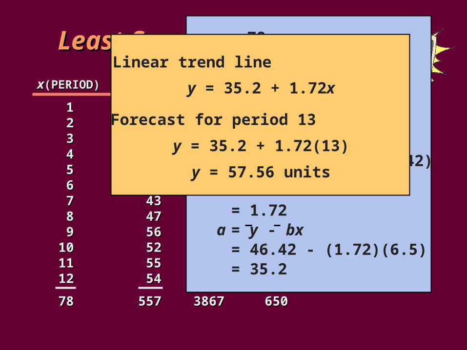
Least Squares ExampleLeast Squares Example
xx(PERIOD)(PERIOD) yy(DEMAND)(DEMAND) xyxy xx22
11 7373 3737 1122 4040 8080 4433 4141 123123 9944 3737 148148 161655 4545 225225 252566 5050 300300 363677 4343 301301 494988 4747 376376 646499 5656 504504 8181
1010 5252 520520 1001001111 5555 605605 1211211212 5454 648648 144144
7878 557557 38673867 650650
x = = 6.5
y = = 46.42
b =
=
= 1.72a = y - bx
= 46.42 - (1.72)(6.5)= 35.2
3867 - (12)(6.5)(46.42)650 - 12(6.5)2
xy - nxyx2 - nx2
781255712
Linear trend line
y = 35.2 + 1.72x
Forecast for period 13
y = 35.2 + 1.72(13)
y = 57.56 units

Linear Trend LineLinear Trend Line
70 70 –
60 60 –
50 50 –
40 40 –
30 30 –
20 20 –
1010 –
0 0 –| | | | | | | | | | | | |11 22 33 44 55 66 77 88 99 1010 1111 1212 1313
Dem
and
Dem
and
PeriodPeriod
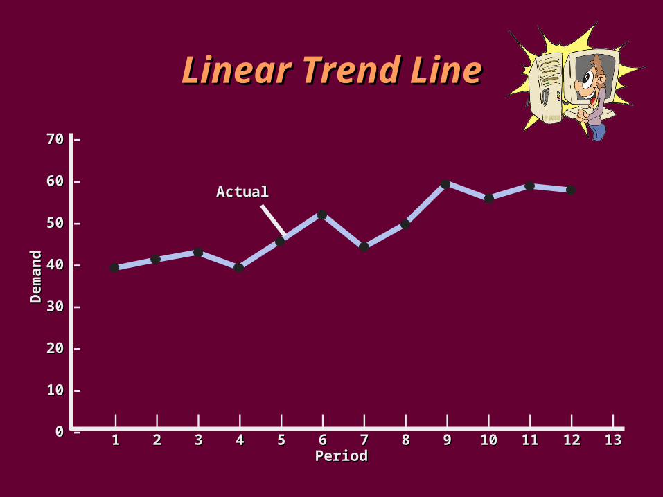
Linear Trend LineLinear Trend Line
70 70 –
60 60 –
50 50 –
40 40 –
30 30 –
20 20 –
1010 –
0 0 –| | | | | | | | | | | | |11 22 33 44 55 66 77 88 99 1010 1111 1212 1313
ActualActual
Dem
and
Dem
and
PeriodPeriod

Linear Trend LineLinear Trend Line
70 70 –
60 60 –
50 50 –
40 40 –
30 30 –
20 20 –
1010 –
0 0 –| | | | | | | | | | | | |11 22 33 44 55 66 77 88 99 1010 1111 1212 1313
ActualActual
Dem
and
Dem
and
PeriodPeriod
Linear trend lineLinear trend line

Trend-Trend-Adjusted Exponential Adjusted Exponential SmoothingSmoothing
A variation of simple exponential smoothing can be used when a time series exhibits trend and it is called trend-adjusted exponential smoothing or double smoothing
If a series exhibits trend, and simple smoothing is used on it the forecasts will all lag the trend: if the data are increasing, each forecast will be too low; if the data are decreasing, each forecast will be too high.
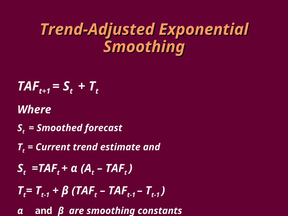
Trend-Trend-Adjusted Exponential Adjusted Exponential SmoothingSmoothing
TAFt+1 = St + Tt
Where
St = Smoothed forecast
Tt = Current trend estimate and
St =TAFt + α (At – TAFt )
Tt= Tt-1 + β (TAFt – TAFt-1 – Tt-1 )
α and β are smoothing constants
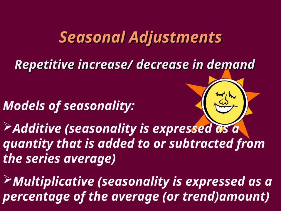
Seasonal AdjustmentsSeasonal Adjustments
Repetitive increase/ decrease in demandRepetitive increase/ decrease in demand
Models of seasonality:
Additive (seasonality is expressed as a quantity that is added to or subtracted from the series average)
Multiplicative (seasonality is expressed as a percentage of the average (or trend)amount)
Seasonal AdjustmentsSeasonal Adjustments
The seasonal percentages The seasonal percentages in the multiplicative in the multiplicative model are referred to as model are referred to as seasonal relatives or seasonal relatives or seasonal indexesseasonal indexes
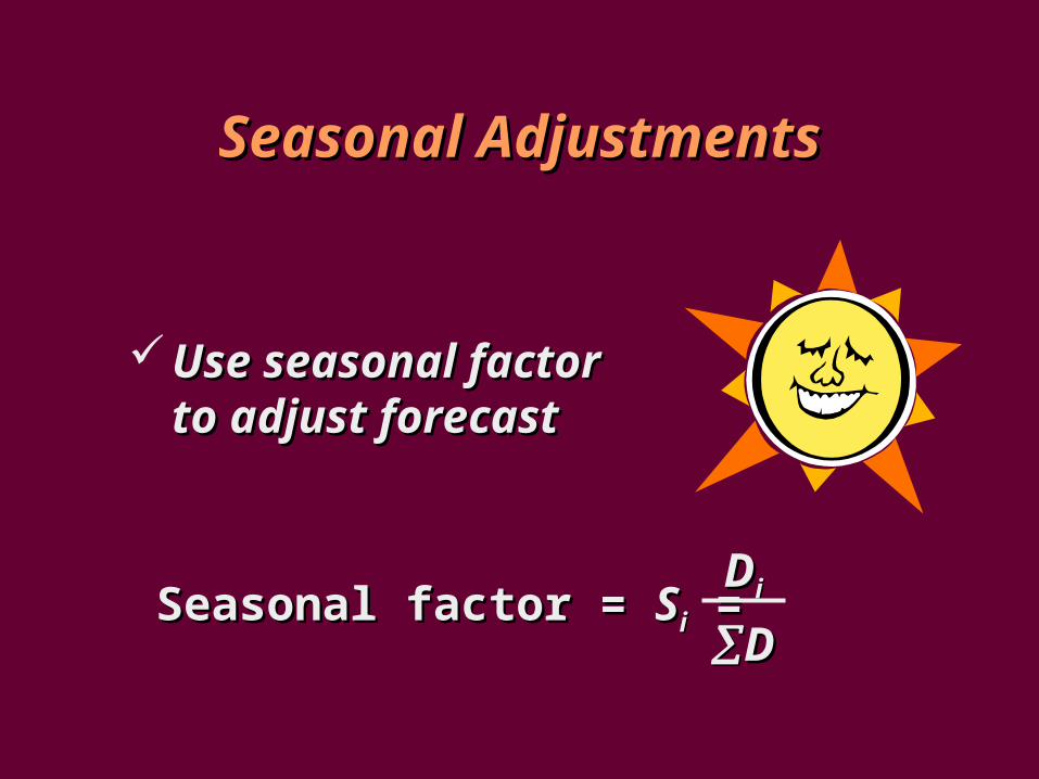
Seasonal AdjustmentsSeasonal Adjustments
Use seasonal factor Use seasonal factor to adjust forecastto adjust forecast
Seasonal factor = Seasonal factor = SSii = =DDii
DD

Seasonal AdjustmentSeasonal Adjustment
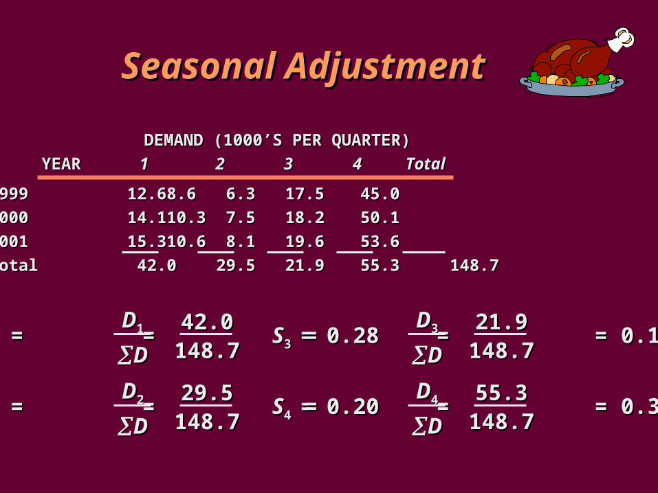
1999 12.61999 12.6 8.68.6 6.36.3 17.517.5 45.045.0
2000 14.12000 14.1 10.310.3 7.57.5 18.218.2 50.150.1
2001 15.32001 15.3 10.610.6 8.18.1 19.619.6 53.653.6
Total 42.0Total 42.0 29.529.5 21.921.9 55.355.3 148.7148.7
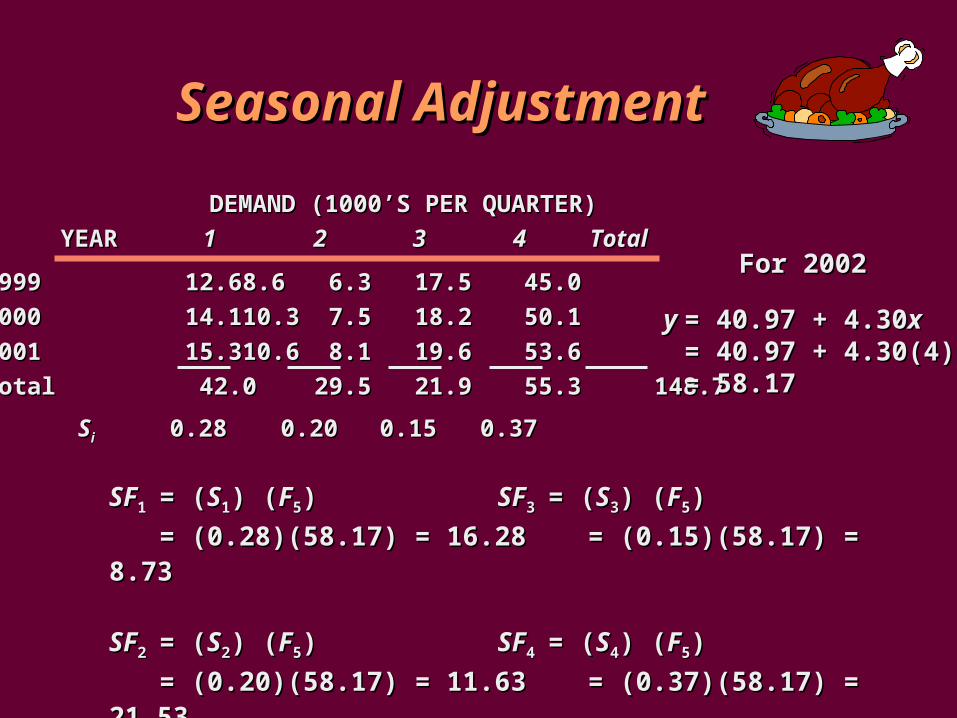
DEMAND (1000’S PER QUARTER)DEMAND (1000’S PER QUARTER)
YEARYEAR 11 22 33 44 TotalTotal
Seasonal AdjustmentSeasonal Adjustment
1999 12.61999 12.6 8.68.6 6.36.3 17.517.5 45.045.0
2000 14.12000 14.1 10.310.3 7.57.5 18.218.2 50.150.1
2001 15.32001 15.3 10.610.6 8.18.1 19.619.6 53.653.6
Total 42.0Total 42.0 29.529.5 21.921.9 55.355.3 148.7148.7
DEMAND (1000’S PER QUARTER)DEMAND (1000’S PER QUARTER)
YEARYEAR 11 22 33 44 TotalTotal
SS11 = = = 0.28 = = = 0.28 DD11
DD
42.042.0148.7148.7
SS22 = = = 0.20 = = = 0.20 DD22
DD
29.529.5148.7148.7
SS44 = = = 0.37 = = = 0.37 DD44
DD
55.355.3148.7148.7
SS33 = = = 0.15 = = = 0.15 DD33
DD
21.921.9148.7148.7
Seasonal AdjustmentSeasonal Adjustment
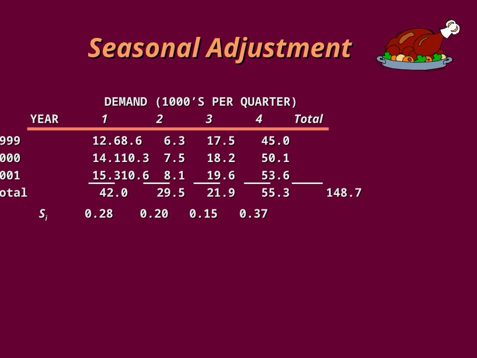
1999 12.61999 12.6 8.68.6 6.36.3 17.517.5 45.045.0
2000 14.12000 14.1 10.310.3 7.57.5 18.218.2 50.150.1
2001 15.32001 15.3 10.610.6 8.18.1 19.619.6 53.653.6
Total 42.0Total 42.0 29.529.5 21.921.9 55.355.3 148.7148.7
DEMAND (1000’S PER QUARTER)DEMAND (1000’S PER QUARTER)
YEARYEAR 11 22 33 44 TotalTotal
SSii 0.280.28 0.200.20 0.150.15 0.370.37
Seasonal AdjustmentSeasonal Adjustment
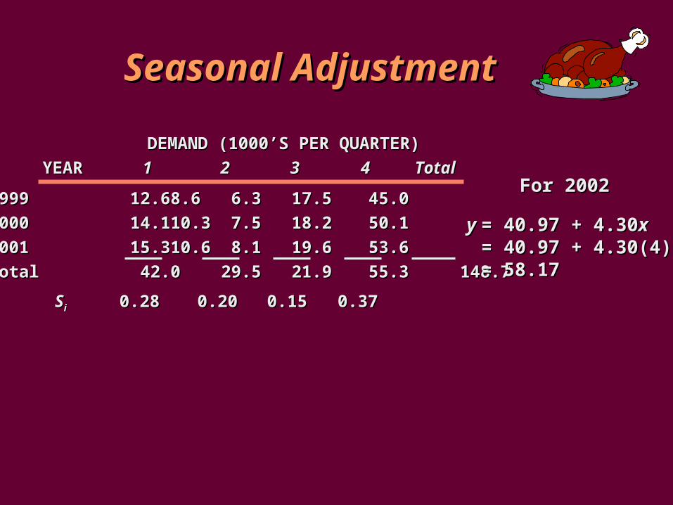
1999 12.61999 12.6 8.68.6 6.36.3 17.517.5 45.045.0
2000 14.12000 14.1 10.310.3 7.57.5 18.218.2 50.150.1
2001 15.32001 15.3 10.610.6 8.18.1 19.619.6 53.653.6
Total 42.0Total 42.0 29.529.5 21.921.9 55.355.3 148.7148.7
DEMAND (1000’S PER QUARTER)DEMAND (1000’S PER QUARTER)
YEARYEAR 11 22 33 44 TotalTotal
SSii 0.280.28 0.200.20 0.150.15 0.370.37
yy = 40.97 + 4.30= 40.97 + 4.30xx= 40.97 + 4.30(4)= 40.97 + 4.30(4)= 58.17= 58.17
For 2002For 2002
Seasonal AdjustmentSeasonal Adjustment
SFSF11 = (= (SS11) () (FF55)) SFSF33 = (= (SS33) () (FF55) )
= (0.28)(58.17) = 16.28= (0.28)(58.17) = 16.28 = (0.15)(58.17) = 8.73= (0.15)(58.17) = 8.73
SFSF22 = (= (SS22) () (FF55)) SFSF44 = (= (SS44) () (FF55) )
= (0.20)(58.17) = 11.63= (0.20)(58.17) = 11.63 = (0.37)(58.17) = 21.53= (0.37)(58.17) = 21.53
1999 12.61999 12.6 8.68.6 6.36.3 17.517.5 45.045.0
2000 14.12000 14.1 10.310.3 7.57.5 18.218.2 50.150.1
2001 15.32001 15.3 10.610.6 8.18.1 19.619.6 53.653.6
Total 42.0Total 42.0 29.529.5 21.921.9 55.355.3 148.7148.7
DEMAND (1000’S PER QUARTER)DEMAND (1000’S PER QUARTER)
YEARYEAR 11 22 33 44 TotalTotal
SSii 0.280.28 0.200.20 0.150.15 0.370.37
yy = 40.97 + 4.30= 40.97 + 4.30xx= 40.97 + 4.30(4)= 40.97 + 4.30(4)= 58.17= 58.17
For 2002For 2002
Centered Moving AverageCentered Moving Average
A commonly used method for representing the trend portion of a time series involves a centered moving average.
By virtue of its centered position it looks forward and looks backward, so it is able to closely follow data movements whether they involve trends, cycles, or random variability alone.
Computing Seasonal Relatives Computing Seasonal Relatives by Using Centered Moving by Using Centered Moving
AveragesAverages The ratio of demand at period i to the
centered average at period i is an estimate of the seasonal relative at that point.
Associative ForecastingAssociative Forecasting
Predictor variables - used to predict values of variable interest
Regression - technique for fitting a line to a set of points
Least squares line - minimizes sum of squared deviations around the line
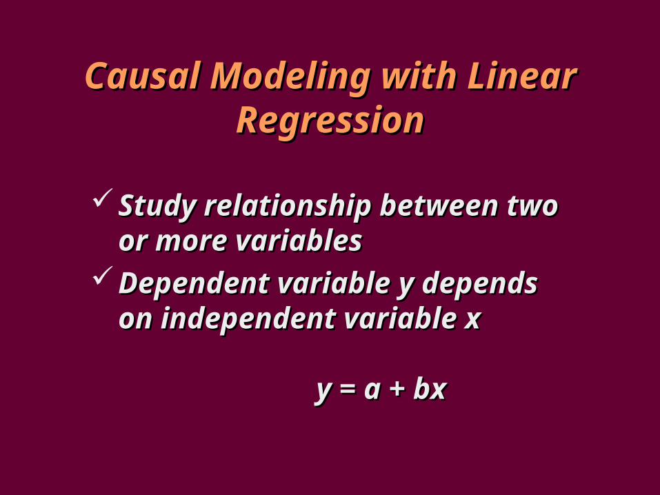
Causal Modeling with Linear Causal Modeling with Linear RegressionRegression
Study relationship between two Study relationship between two or more variablesor more variables
Dependent variable Dependent variable yy depends depends on independent variable on independent variable xx
yy = = aa + + bxbx
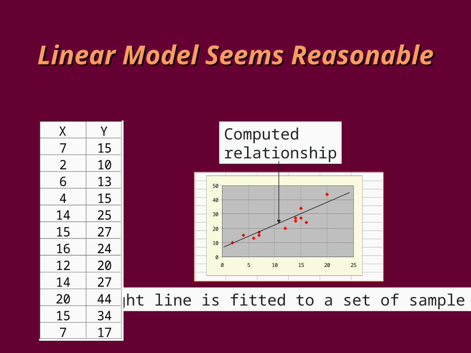
Linear Model Seems ReasonableLinear Model Seems Reasonable
A straight line is fitted to a set of sample points.
0
10
20
30
40
50
0 5 10 15 20 25
X Y7 152 106 134 15
14 2515 2716 2412 2014 2720 4415 347 17
Computedrelationship
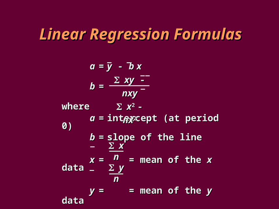
Linear Regression FormulasLinear Regression Formulas
aa == yy - - b xb x
bb ==
wherewhereaa == intercept (at period 0)intercept (at period 0)bb == slope of the line slope of the line
xx == = mean of the = mean of the xx data data
yy == = mean of the = mean of the yy data data
xyxy - -
nxynxy
xx22 - - nxnx22
xxnn
yynn
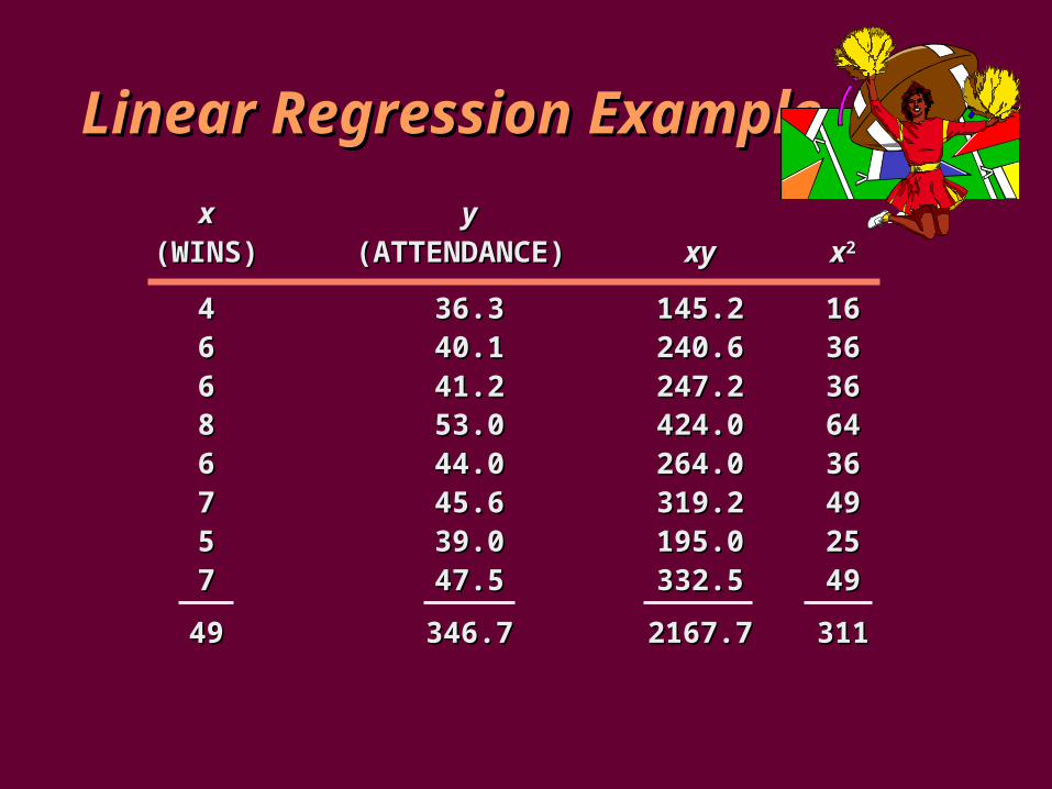
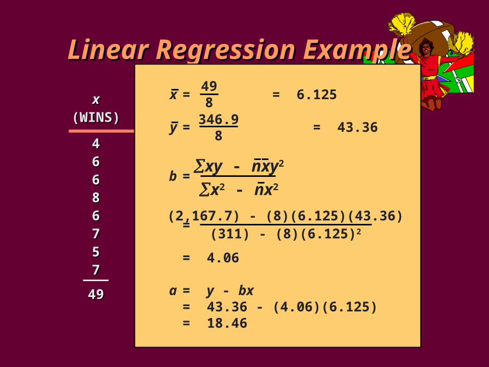
Linear Regression ExampleLinear Regression Example
xx yy(WINS)(WINS) (ATTENDANCE) (ATTENDANCE) xyxy xx22
44 36.336.3 145.2145.2 161666 40.140.1 240.6240.6 363666 41.241.2 247.2247.2 363688 53.053.0 424.0424.0 646466 44.044.0 264.0264.0 363677 45.645.6 319.2319.2 494955 39.039.0 195.0195.0 252577 47.547.5 332.5332.5 4949
4949 346.7346.7 2167.72167.7 311311
x = = 6.125
y = = 43.36
b =
=
= 4.06
a = y - bx= 43.36 - (4.06)(6.125)= 18.46
498
346.98
xy - nxy2
x2 - nx2
(2,167.7) - (8)(6.125)(43.36)(311) - (8)(6.125)2
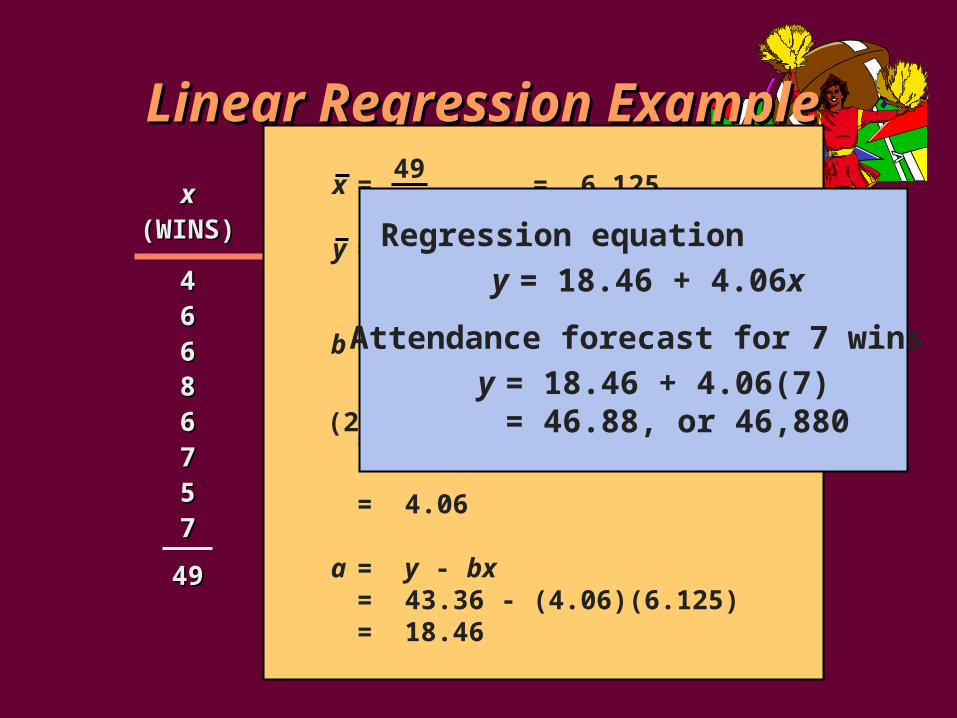
y = 18.46 + 4.06x
y = 18.46 + 4.06(7)= 46.88, or 46,880
Regression equation
Attendance forecast for 7 wins
Linear Regression LineLinear Regression Line60,000 60,000 –
50,000 50,000 –
40,000 40,000 –
30,000 30,000 –
20,000 20,000 –
10,000 10,000 –
| | | | | | | | | | |00 11 22 33 44 55 66 77 88 99 1010
Wins, x
Att
end
ance
, y
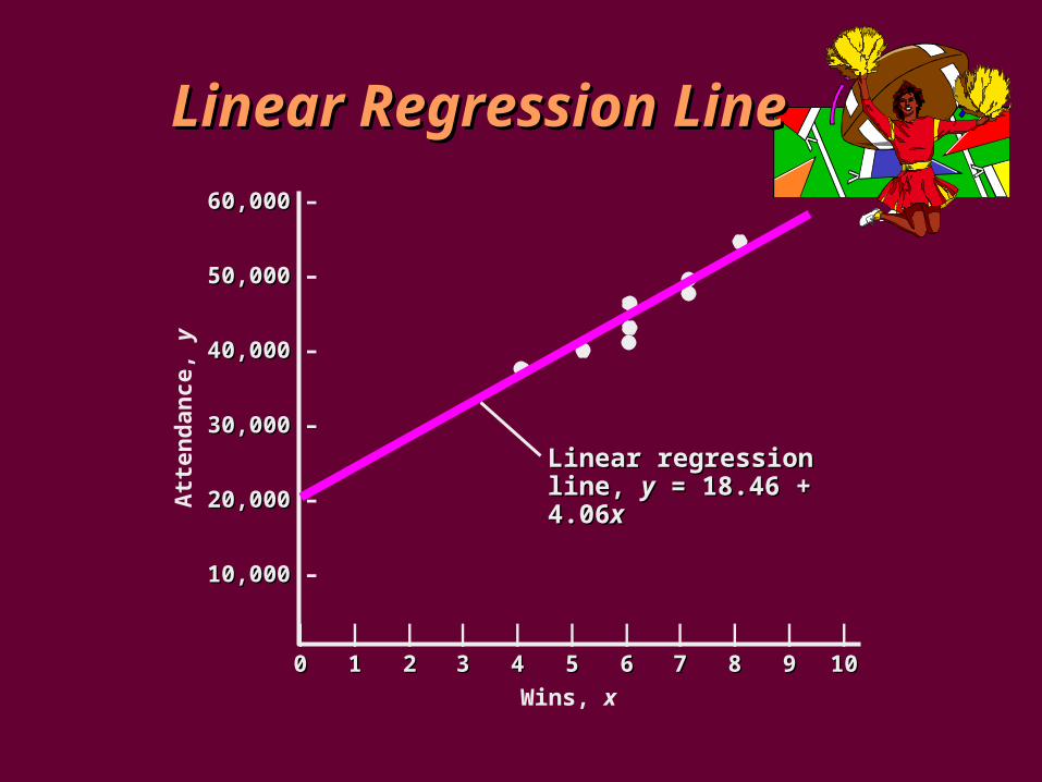
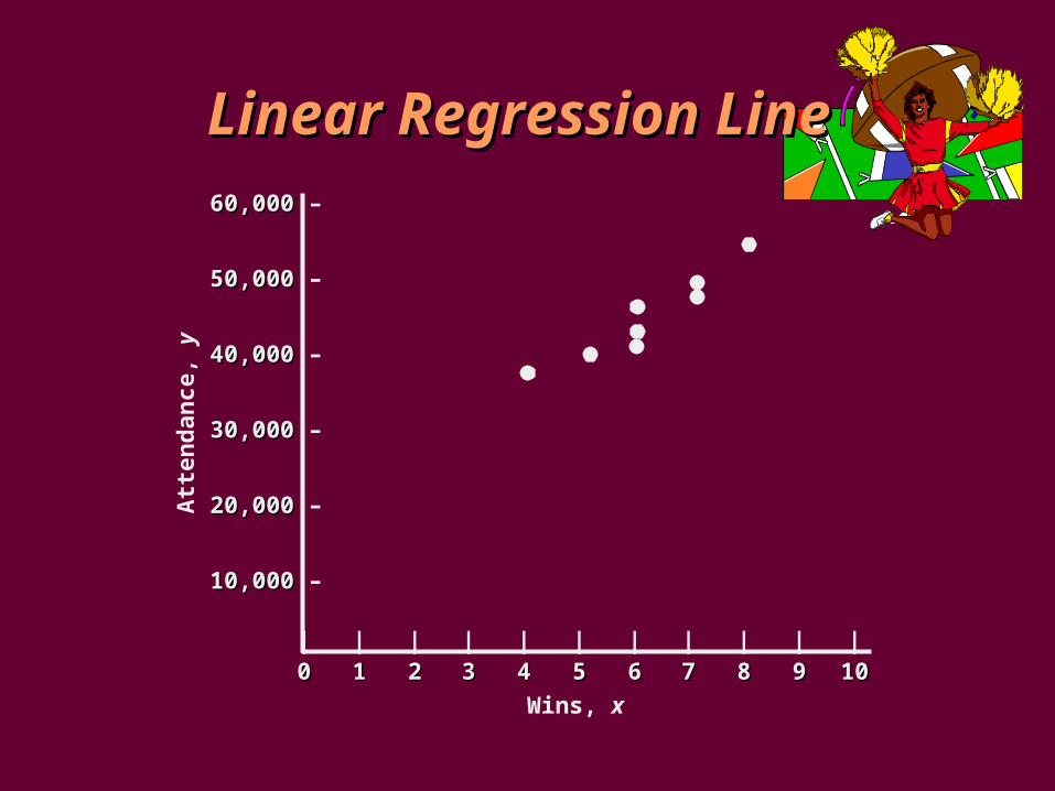
Linear Regression LineLinear Regression Line
| | | | | | | | | | |00 11 22 33 44 55 66 77 88 99 1010
60,000 60,000 –
50,000 50,000 –
40,000 40,000 –
30,000 30,000 –
20,000 20,000 –
10,000 10,000 –
Linear regression line, Linear regression line, yy = 18.46 + 4.06 = 18.46 + 4.06xx
Wins, x
Att
end
ance
, y
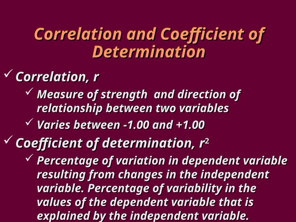
Correlation and Coefficient of Correlation and Coefficient of DeterminationDetermination
Correlation, Correlation, rr Measure of strength Measure of strength and direction and direction of of
relationshiprelationship between two variables between two variables Varies between -1.00 and +1.00Varies between -1.00 and +1.00
Coefficient of determination, Coefficient of determination, rr22
Percentage of variation in dependent variable Percentage of variation in dependent variable resulting from changes in the independent resulting from changes in the independent variablevariable. Percentage of variability in the values . Percentage of variability in the values of the dependent variable that is explained by of the dependent variable that is explained by the independent variable. the independent variable.

Computing CorrelationComputing Correlation
nn xyxy - - xx yy
[[nn xx22 - ( - ( xx))22] [] [nn yy22 - ( - ( yy))22]]r r ==
Coefficient of determination Coefficient of determination rr2 2 = (0.947)= (0.947)2 2 = 0.897= 0.897
r r ==(8)(2,167.7) - (49)(346.9)(8)(2,167.7) - (49)(346.9)
[[(8)(311) - (49(8)(311) - (49)2)2] [] [(8)(15,224.7) - (346.9)(8)(15,224.7) - (346.9)22]]
rr = 0.947 = 0.947
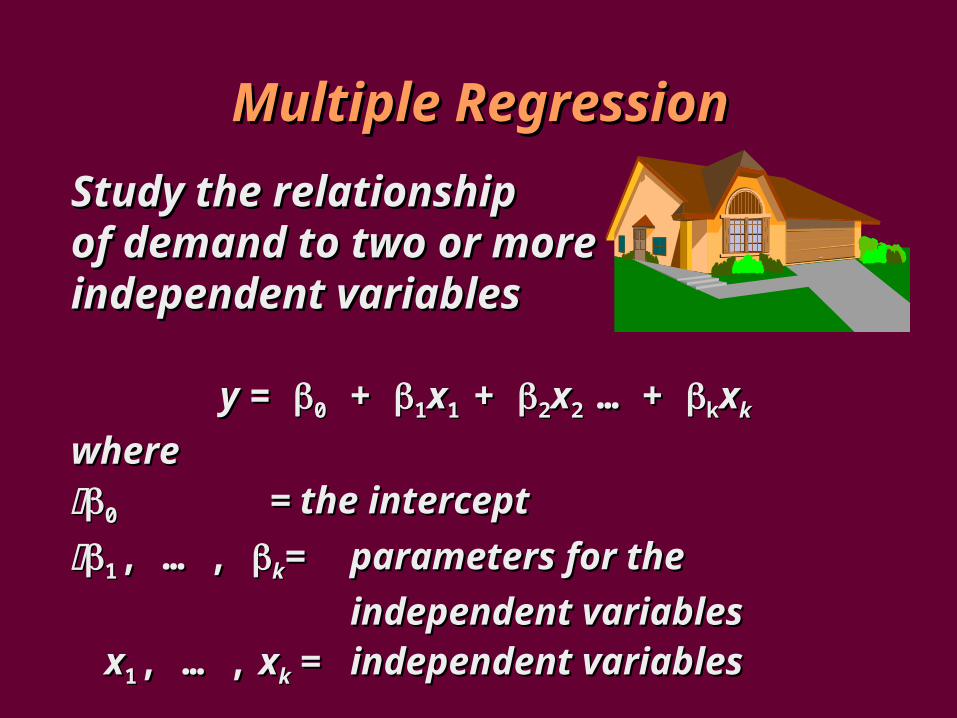
Multiple RegressionMultiple Regression
Study the relationship Study the relationship of demand to two or more of demand to two or more independent variablesindependent variables
y y = = 00 + + 11xx1 1 + + 22xx2 2 … + … + kkxxkk
wherewhere00 == the interceptthe intercept
11, … , , … , kk == parameters for theparameters for the
independent variablesindependent variablesxx11, … ,, … , xxkk == independent variablesindependent variables
Important Points in Using Important Points in Using RegressionRegression
Always plot the data to verify that a linear relationship is appropriate
Check whether the data is time-dependent. I f so use time series instead of regression
A small correlation may imply that other variables are important

Forecast AccuracyForecast Accuracy
Error = Actual - ForecastError = Actual - ForecastFind a method which minimizes Find a method which minimizes
errorerrorMean Absolute Mean Absolute
Deviation (MAD)Deviation (MAD)Mean Squared Error (MSE)Mean Squared Error (MSE)Mean Absolute Mean Absolute
Percent Deviation (MAPPercent Deviation (MAPEE))
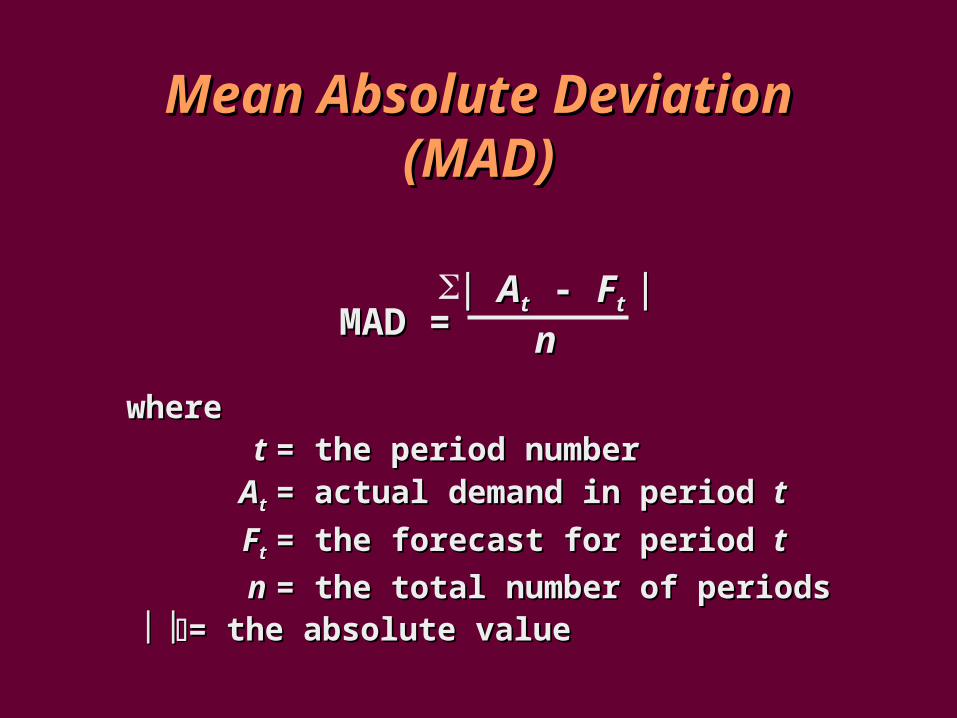
Mean Absolute Deviation Mean Absolute Deviation (MAD)(MAD)
wherewhere tt = the period number= the period number
AAtt = = actual actual demand in period demand in period tt
FFtt = the forecast for period = the forecast for period tt
nn = the total number of periods= the total number of periods= the absolute value= the absolute value
AAtt - - FFtt nnMAD =MAD =
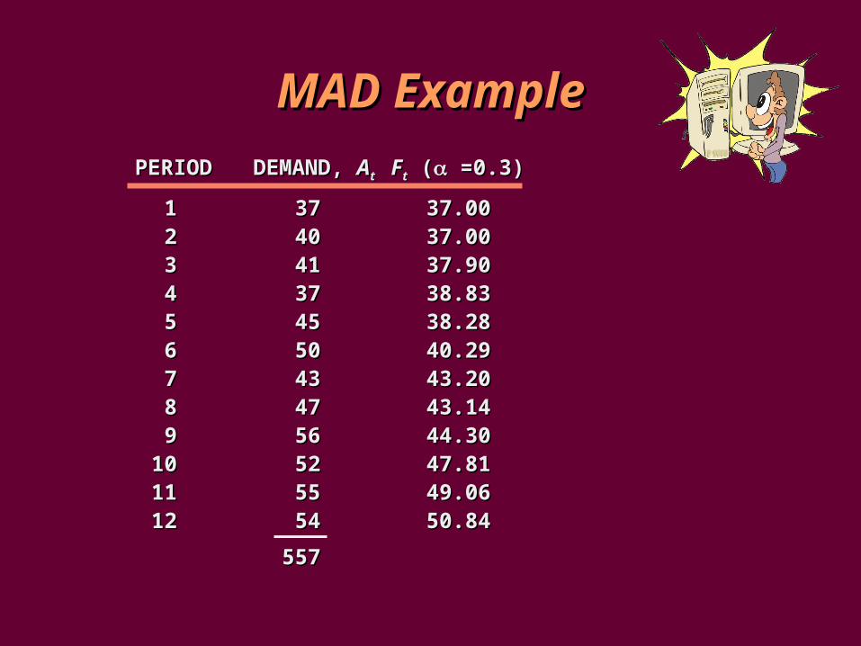
MAD ExampleMAD Example
11 3737 37.0037.0022 4040 37.0037.0033 4141 37.9037.9044 3737 38.8338.8355 4545 38.2838.2866 5050 40.2940.2977 4343 43.2043.2088 4747 43.1443.1499 5656 44.3044.30
1010 5252 47.8147.811111 5555 49.0649.061212 5454 50.8450.84
557557
PERIODPERIOD DEMAND, DEMAND, AAtt FFtt ( ( =0.3) =0.3)

MAD ExampleMAD Example
11 3737 37.0037.00 –– ––22 4040 37.0037.00 3.003.00 3.003.0033 4141 37.9037.90 3.103.10 3.103.1044 3737 38.8338.83 -1.83-1.83 1.831.8355 4545 38.2838.28 6.726.72 6.726.7266 5050 40.2940.29 9.699.69 9.699.6977 4343 43.2043.20 -0.20-0.20 0.200.2088 4747 43.1443.14 3.863.86 3.863.8699 5656 44.3044.30 11.7011.70 11.7011.70
1010 5252 47.8147.81 4.194.19 4.194.191111 5555 49.0649.06 5.945.94 5.945.941212 5454 50.8450.84 3.153.15 3.153.15
557557 49.3149.31 53.3953.39
PERIODPERIOD DEMAND, DEMAND, AAtt FFtt ( ( =0.3) =0.3) ((AAtt - - FFtt)) | |AAtt - - FFtt||
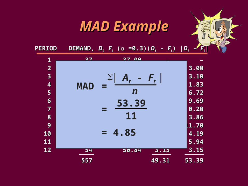
MAD ExampleMAD Example
11 3737 37.0037.00 –– ––22 4040 37.0037.00 3.003.00 3.003.0033 4141 37.9037.90 3.103.10 3.103.1044 3737 38.8338.83 -1.83-1.83 1.831.8355 4545 38.2838.28 6.726.72 6.726.7266 5050 40.2940.29 9.699.69 9.699.6977 4343 43.2043.20 -0.20-0.20 0.200.2088 4747 43.1443.14 3.863.86 3.863.8699 5656 44.3044.30 11.7011.70 11.7011.70
1010 5252 47.8147.81 4.194.19 4.194.191111 5555 49.0649.06 5.945.94 5.945.941212 5454 50.8450.84 3.153.15 3.153.15
557557 49.3149.31 53.3953.39
PERIODPERIOD DEMAND, DEMAND, DDtt FFtt ( ( =0.3) =0.3) ((DDtt - - FFtt)) | |DDtt - - FFtt||
At - Ft nMAD =
=
= 4.85
53.3911
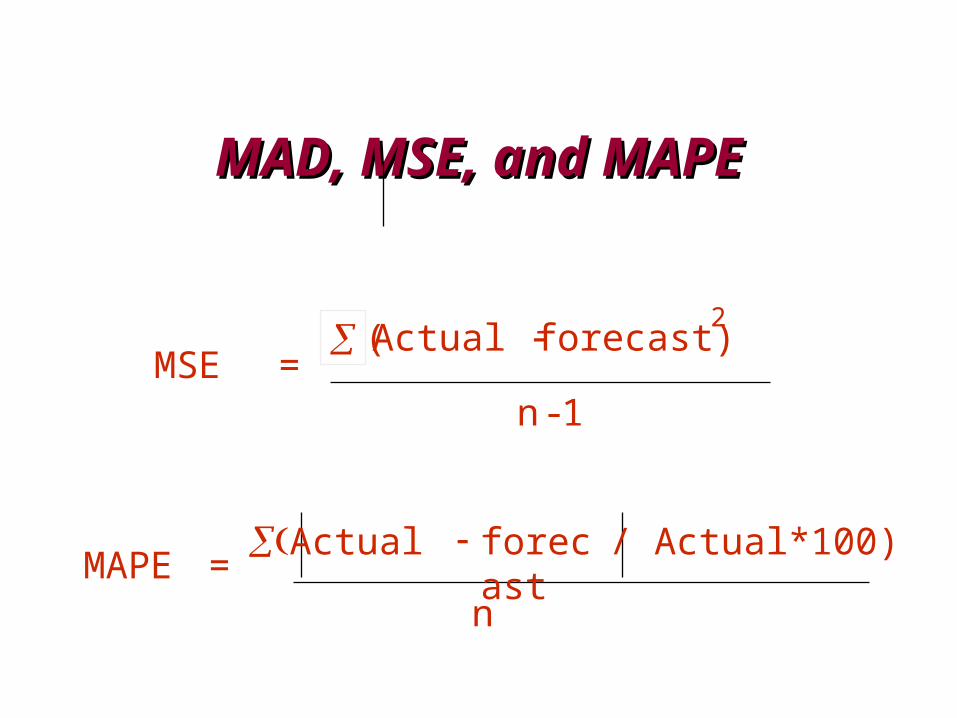
MAD, MSE, and MAPEMAD, MSE, and MAPE
MSE = Actual forecast)
-1
2
n
(
MAPE = Actual forecas
t
n
/ Actual*100)

Example 10Example 10
Period Actual Forecast (A-F) |A-F| (A-F)^2 (|A-F|/Actual)*1001 217 215 2 2 4 0.922 213 216 -3 3 9 1.413 216 215 1 1 1 0.464 210 214 -4 4 16 1.905 213 211 2 2 4 0.946 219 214 5 5 25 2.287 216 217 -1 1 1 0.468 212 216 -4 4 16 1.89
-2 22 76 10.26
MAD= 2.75MSE= 10.86
MAPE= 1.28
Forecast ControlForecast Control
Reasons for out-of-control forecastsReasons for out-of-control forecasts
(sources of forecast errors) (sources of forecast errors) Change in trendChange in trend Appearance of cycleAppearance of cycle Inadequate forecastsInadequate forecasts Irregular variationsIrregular variations Incorrect use of forecasting techniqueIncorrect use of forecasting technique

Controlling the ForecastControlling the Forecast
A forecast is deemed to perform adequately when the errors exhibit only random variations
• Control chart– A visual tool for monitoring forecast errors– Used to detect non-randomness in errors
• Forecasting errors are in control if– All errors are within the control limits– No patterns, such as trends or cycles, are
present
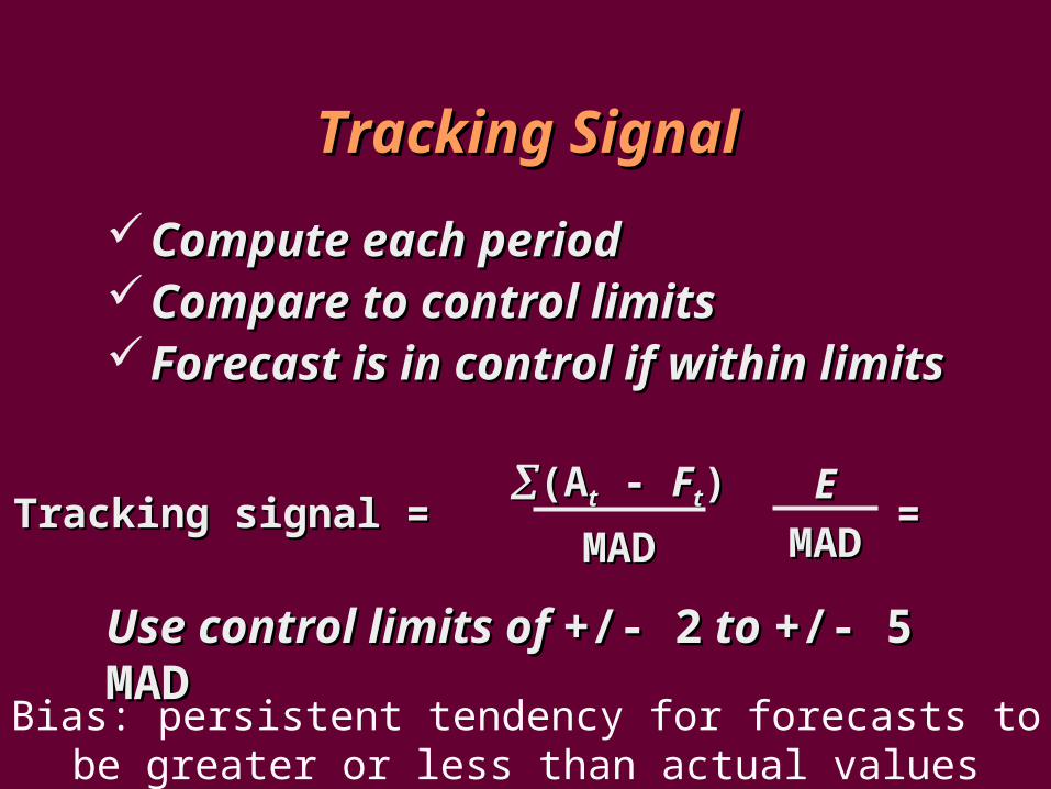
Tracking SignalTracking Signal
Compute each periodCompute each periodCompare to control limitsCompare to control limitsForecast is in control if within limitsForecast is in control if within limits
Use control limits of Use control limits of +/- 2+/- 2 to to +/- 5 +/- 5 MADMAD
Tracking signal = =Tracking signal = =((AAtt - - FFtt))
MADMAD
EE
MADMAD
Bias: persistent tendency for forecasts to be greater or less than actual values

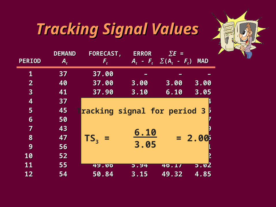
Tracking Signal ValuesTracking Signal Values
11 3737 37.0037.00 –– –– ––22 4040 37.0037.00 3.003.00 3.003.00 3.003.0033 4141 37.9037.90 3.103.10 6.106.10 3.053.0544 3737 38.8338.83 -1.83-1.83 4.274.27 2.642.6455 4545 38.2838.28 6.726.72 10.9910.99 3.663.6666 5050 40.2940.29 9.699.69 20.6820.68 4.874.8777 4343 43.2043.20 -0.20-0.20 20.4820.48 4.094.0988 4747 43.1443.14 3.863.86 24.3424.34 4.064.0699 5656 44.3044.30 11.7011.70 36.0436.04 5.015.01
1010 5252 47.8147.81 4.194.19 40.2340.23 4.924.921111 5555 49.0649.06 5.945.94 46.1746.17 5.025.021212 5454 50.8450.84 3.153.15 49.3249.32 4.854.85
DEMANDDEMAND FORECAST,FORECAST, ERRORERROR EE = =PERIODPERIOD DDtt FFtt AAtt - - FFtt ((AAtt - - FFtt)) MADMAD
Tracking Signal ValuesTracking Signal Values
11 3737 37.0037.00 –– –– ––22 4040 37.0037.00 3.003.00 3.003.00 3.003.0033 4141 37.9037.90 3.103.10 6.106.10 3.053.0544 3737 38.8338.83 -1.83-1.83 4.274.27 2.642.6455 4545 38.2838.28 6.726.72 10.9910.99 3.663.6666 5050 40.2940.29 9.699.69 20.6820.68 4.874.8777 4343 43.2043.20 -0.20-0.20 20.4820.48 4.094.0988 4747 43.1443.14 3.863.86 24.3424.34 4.064.0699 5656 44.3044.30 11.7011.70 36.0436.04 5.015.01
1010 5252 47.8147.81 4.194.19 40.2340.23 4.924.921111 5555 49.0649.06 5.945.94 46.1746.17 5.025.021212 5454 50.8450.84 3.153.15 49.3249.32 4.854.85
DEMANDDEMAND FORECAST,FORECAST, ERRORERROR EE = =PERIODPERIOD AAtt FFtt AAtt - - FFtt ((AAtt - - FFtt)) MADMAD
TS3 = = 2.006.103.05
Tracking signal for period 3
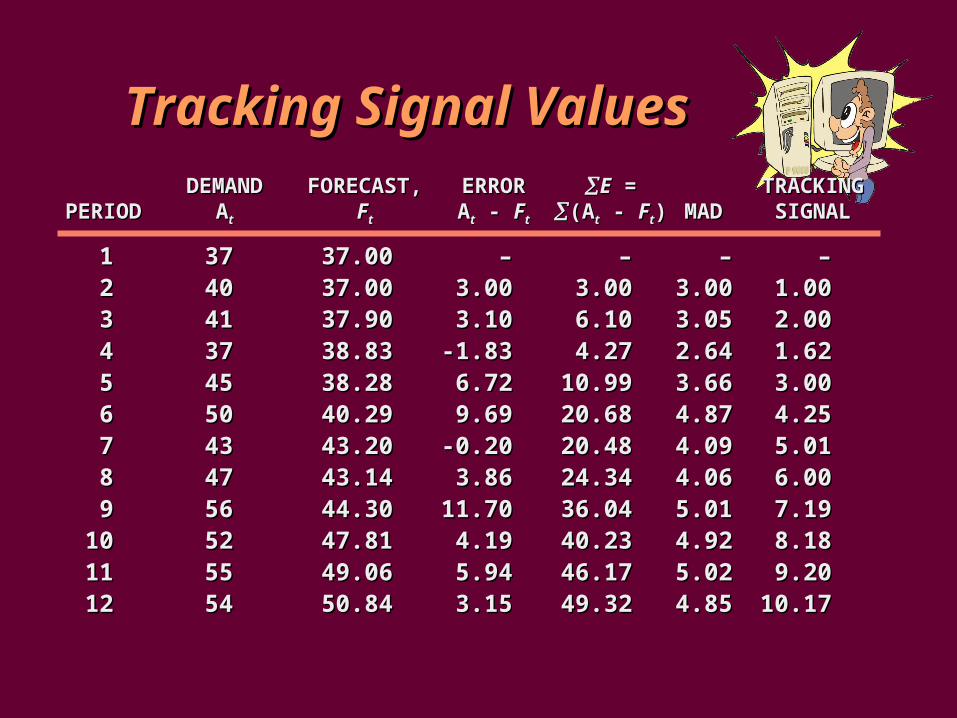
Tracking Signal ValuesTracking Signal Values
11 3737 37.0037.00 –– –– –– ––22 4040 37.0037.00 3.003.00 3.003.00 3.003.00 1.001.0033 4141 37.9037.90 3.103.10 6.106.10 3.053.05 2.002.0044 3737 38.8338.83 -1.83-1.83 4.274.27 2.642.64 1.621.6255 4545 38.2838.28 6.726.72 10.9910.99 3.663.66 3.003.0066 5050 40.2940.29 9.699.69 20.6820.68 4.874.87 4.254.2577 4343 43.2043.20 -0.20-0.20 20.4820.48 4.094.09 5.015.0188 4747 43.1443.14 3.863.86 24.3424.34 4.064.06 6.006.0099 5656 44.3044.30 11.7011.70 36.0436.04 5.015.01 7.197.19
1010 5252 47.8147.81 4.194.19 40.2340.23 4.924.92 8.188.181111 5555 49.0649.06 5.945.94 46.1746.17 5.025.02 9.209.201212 5454 50.8450.84 3.153.15 49.3249.32 4.854.85 10.1710.17
DEMANDDEMAND FORECAST,FORECAST, ERRORERROR EE = = TRACKINGTRACKINGPERIODPERIOD AAtt FFtt AAtt - - FFtt ((AAtt - - FFtt)) MADMAD SIGNALSIGNAL
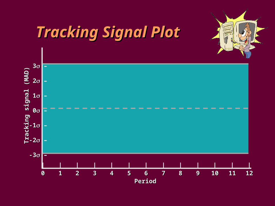
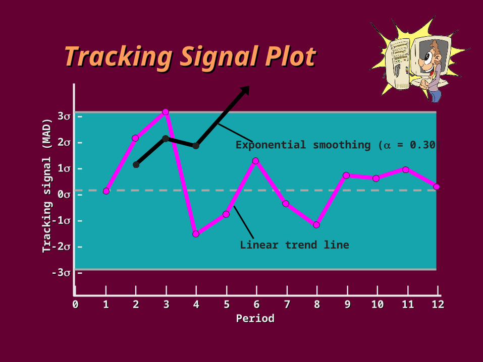
Tracking Signal PlotTracking Signal Plot
33 –
22 –
11 –
00 –
-1-1 –
-2-2 –
-3-3 –
| | | | | | | | | | | | |00 11 22 33 44 55 66 77 88 99 1010 1111 1212
Tra
ckin
g s
ign
al (
MA
D)
Tra
ckin
g s
ign
al (
MA
D)
PeriodPeriod

Tracking Signal PlotTracking Signal Plot
33 –
22 –
11 –
00 –
-1-1 –
-2-2 –
-3-3 –
| | | | | | | | | | | | |00 11 22 33 44 55 66 77 88 99 1010 1111 1212
Tra
ckin
g s
ign
al (
MA
D)
Tra
ckin
g s
ign
al (
MA
D)
PeriodPeriod
Exponential smoothing ( = 0.30)
Tracking Signal PlotTracking Signal Plot
33 –
22 –
11 –
00 –
-1-1 –
-2-2 –
-3-3 –
| | | | | | | | | | | | |00 11 22 33 44 55 66 77 88 99 1010 1111 1212
Tra
ckin
g s
ign
al (
MA
D)
Tra
ckin
g s
ign
al (
MA
D)
PeriodPeriod
Exponential smoothing ( = 0.30)
Linear trend line
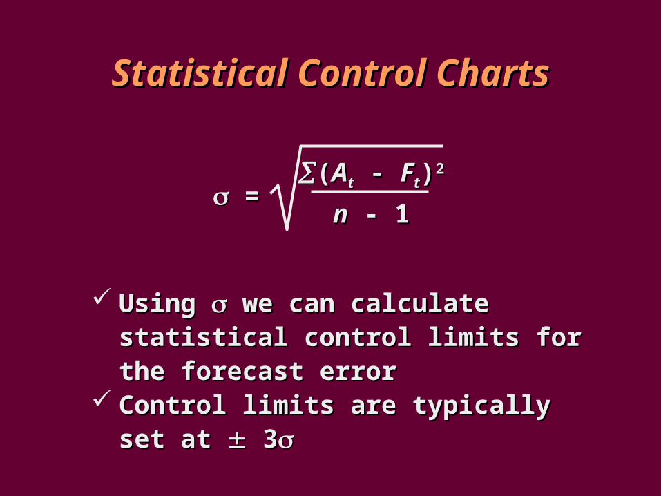
Statistical Control ChartsStatistical Control Charts
==((AAtt - - FFtt))22
nn - 1 - 1
Using Using we can calculate statistical we can calculate statistical control limits for the forecast errorcontrol limits for the forecast error
Control limits are typically set at Control limits are typically set at 3 3
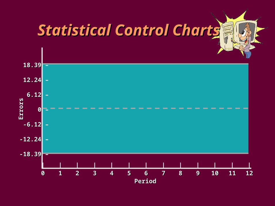
Statistical Control ChartsStatistical Control ChartsE
rro
rsE
rro
rs
18.39 18.39 –
12.24 12.24 –
6.12 6.12 –
0 0 –
-6.12 -6.12 –
-12.24 -12.24 –
-18.39 -18.39 –
| | | | | | | | | | | | |00 11 22 33 44 55 66 77 88 99 1010 1111 1212
PeriodPeriod
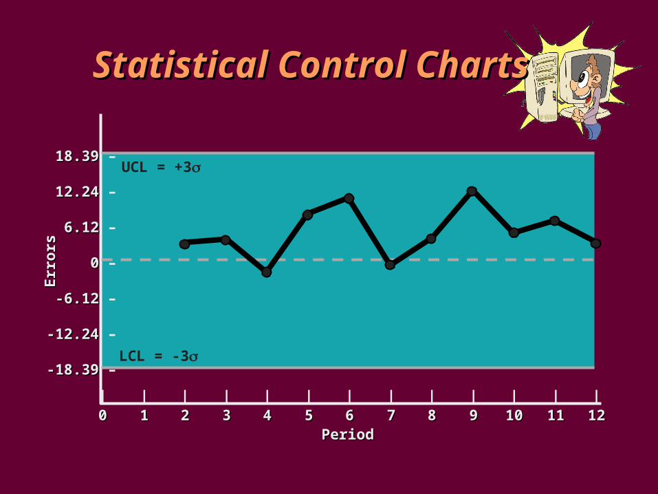
Statistical Control ChartsStatistical Control ChartsE
rro
rsE
rro
rs
18.39 18.39 –
12.24 12.24 –
6.12 6.12 –
0 0 –
-6.12 -6.12 –
-12.24 -12.24 –
-18.39 -18.39 –
| | | | | | | | | | | | |00 11 22 33 44 55 66 77 88 99 1010 1111 1212
PeriodPeriod
UCL = +3
LCL = -3
Choosing a Forecasting TechniqueChoosing a Forecasting Technique
• No single technique works in every situation
• Two most important factors– Cost– Accuracy
• Other factors include the availability of:– Historical data– Computers– Time needed to gather and analyze the data– Forecast horizon