4 – 1 psm10 © 2006 prentice hall, inc. powerpoint presentation to accompany heizer/render...
TRANSCRIPT

4 4 –– 11PSM10PSM10© 2006 Prentice Hall, Inc.
PowerPoint presentation to accompanyPowerPoint presentation to accompany Heizer/Render Heizer/Render Operations Management, 8e Operations Management, 8e
Chapter 4 – ForecastingChapter 4 – Forecasting

4 4 –– 22PSM10PSM10
What is Forecasting?What is Forecasting?
Process of Process of predicting a future predicting a future eventevent
Underlying basis of Underlying basis of
all business all business decisionsdecisions ProductionProduction
InventoryInventory
PersonnelPersonnel
FacilitiesFacilities
??

4 4 –– 33PSM10PSM10
Forecasting Time HorizonsForecasting Time Horizons
Short-range forecastShort-range forecast Up to 1 year, generally less than 3 monthsUp to 1 year, generally less than 3 months Purchasing, job scheduling, workforce Purchasing, job scheduling, workforce
levels, job assignments, production levelslevels, job assignments, production levels
Medium-range forecastMedium-range forecast 3 months to 3 years3 months to 3 years Sales and production planning, budgetingSales and production planning, budgeting
Long-range forecastLong-range forecast 33++ years years New product planning, facility location, New product planning, facility location,
research and developmentresearch and development

4 4 –– 44PSM10PSM10
Distinguishing DifferencesDistinguishing Differences
Medium/long rangeMedium/long range forecasts deal with forecasts deal with more comprehensive issues and support more comprehensive issues and support management decisions regarding management decisions regarding planning and products, plants and planning and products, plants and processesprocesses
Short-termShort-term forecasting usually employs forecasting usually employs different methodologies than longer-term different methodologies than longer-term forecastingforecasting
Short-termShort-term forecasts tend to be more forecasts tend to be more accurate than longer-term forecastsaccurate than longer-term forecasts

4 4 –– 55PSM10PSM10
Influence of Product Life CycleInfluence of Product Life Cycle
Introduction and growth require longer Introduction and growth require longer forecasts than maturity and declineforecasts than maturity and decline
As product passes through life cycle, As product passes through life cycle, forecasts are useful in projectingforecasts are useful in projecting Staffing levelsStaffing levels
Inventory levelsInventory levels
Factory capacityFactory capacity
Introduction – Growth – Maturity – Decline
4 4 –– 66PSM10PSM10
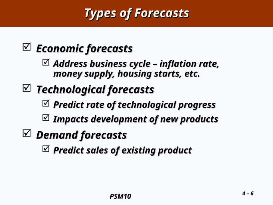
Types of ForecastsTypes of Forecasts
Economic forecastsEconomic forecasts Address business cycle – inflation rate, Address business cycle – inflation rate,
money supply, housing starts, etc.money supply, housing starts, etc.
Technological forecastsTechnological forecasts Predict rate of technological progressPredict rate of technological progress
Impacts development of new productsImpacts development of new products
Demand forecastsDemand forecasts Predict sales of existing productPredict sales of existing product

4 4 –– 77PSM10PSM10
Strategic Importance of ForecastingStrategic Importance of Forecasting
Human Resources – Hiring, training, Human Resources – Hiring, training, laying off workerslaying off workers
Capacity – Capacity shortages can Capacity – Capacity shortages can result in undependable delivery, loss result in undependable delivery, loss of customers, loss of market shareof customers, loss of market share
Supply-Chain Management – Good Supply-Chain Management – Good supplier relations and price advancesupplier relations and price advance

4 4 –– 88PSM10PSM10
Seven Steps in ForecastingSeven Steps in Forecasting
1.1. Determine the use of the forecastDetermine the use of the forecast
2.2. Select the items to be forecastedSelect the items to be forecasted
3.3. Determine the time horizon of the Determine the time horizon of the forecastforecast
4.4. Select the forecasting model(s)Select the forecasting model(s)
5.5. Gather the dataGather the data
6.6. Make the forecastMake the forecast
7.7. Validate and implement resultsValidate and implement results

4 4 –– 99PSM10PSM10
The Realities!The Realities!
Forecasts are seldom perfectForecasts are seldom perfect
Most techniques assume an Most techniques assume an underlying stability in the systemunderlying stability in the system
Product family and aggregated Product family and aggregated forecasts are more accurate than forecasts are more accurate than individual product forecastsindividual product forecasts

4 4 –– 1010PSM10PSM10
Forecasting ApproachesForecasting Approaches
Used when situation is vague Used when situation is vague and little data existand little data exist New productsNew products
New technologyNew technology
Involves intuition, experienceInvolves intuition, experience e.g., forecasting sales on Internete.g., forecasting sales on Internet
Qualitative MethodsQualitative Methods

4 4 –– 1111PSM10PSM10
Forecasting ApproachesForecasting Approaches
Used when situation is ‘stable’ and Used when situation is ‘stable’ and historical data existhistorical data exist Existing productsExisting products
Current technologyCurrent technology
Involves mathematical techniquesInvolves mathematical techniques e.g., forecasting sales of color e.g., forecasting sales of color
televisionstelevisions
Quantitative MethodsQuantitative Methods

4 4 –– 1212PSM10PSM10
Overview of Qualitative MethodsOverview of Qualitative Methods
Jury of executive opinionJury of executive opinion Pool opinions of high-level Pool opinions of high-level
executives, sometimes augment by executives, sometimes augment by statistical modelsstatistical models
Delphi methodDelphi method Panel of experts, queried iterativelyPanel of experts, queried iteratively

4 4 –– 1313PSM10PSM10
Overview of Qualitative MethodsOverview of Qualitative Methods
Sales force compositeSales force composite Estimates from individual Estimates from individual
salespersons are reviewed for salespersons are reviewed for reasonableness, then aggregated reasonableness, then aggregated
Consumer Market SurveyConsumer Market Survey Ask the customerAsk the customer

4 4 –– 1414PSM10PSM10
Involves small group of high-level Involves small group of high-level managersmanagers
Group estimates demand by working Group estimates demand by working togethertogether
Combines managerial experience with Combines managerial experience with statistical modelsstatistical models
Relatively quickRelatively quick
‘‘Group-think’Group-think’disadvantagedisadvantage
Jury of Executive OpinionJury of Executive Opinion

4 4 –– 1515PSM10PSM10
Sales Force CompositeSales Force Composite
Each salesperson projects his or Each salesperson projects his or her salesher sales
Combined at district and national Combined at district and national levelslevels
Sales reps know customers’ wantsSales reps know customers’ wants
Tends to be overly optimisticTends to be overly optimistic

4 4 –– 1616PSM10PSM10
Delphi MethodDelphi Method
Iterative group Iterative group process, process, continues until continues until consensus is consensus is reachedreached
3 types of 3 types of participantsparticipants Decision makersDecision makers StaffStaff RespondentsRespondents
Staff(Administering
survey)
Decision Makers(Evaluate
responses and make decisions)
Respondents(People who can make valuable
judgments)

4 4 –– 1717PSM10PSM10
Consumer Market SurveyConsumer Market Survey
Ask customers about purchasing Ask customers about purchasing plansplans
What consumers say, and what What consumers say, and what they actually do are often differentthey actually do are often different
Sometimes difficult to answerSometimes difficult to answer

4 4 –– 1818PSM10PSM10
Overview of Quantitative ApproachesOverview of Quantitative Approaches
1.1. Naive approachNaive approach
2.2. Moving averagesMoving averages
3.3. Exponential Exponential smoothingsmoothing
4.4. Trend projectionTrend projection
5.5. Linear regressionLinear regression
Time-Series Time-Series ModelsModels
Associative Associative ModelModel

4 4 –– 1919PSM10PSM10
Time Series ForecastingTime Series Forecasting
Set of evenly spaced numerical Set of evenly spaced numerical datadata Obtained by observing response Obtained by observing response
variable at regular time periodsvariable at regular time periods
Forecast based only on past Forecast based only on past valuesvalues Assumes that factors influencing Assumes that factors influencing
past and present will continue past and present will continue influence in futureinfluence in future

4 4 –– 2020PSM10PSM10
Trend
Seasonal
Cyclical
Random
Time Series ComponentsTime Series Components

4 4 –– 2121PSM10PSM10
Components of DemandComponents of DemandD
eman
d f
or
pro
du
ct o
r se
rvic
e
| | | |1 2 3 4
Year
Average demand over four years
Seasonal peaks
Trend component
Actual demand
Random variation
4 4 –– 2222PSM10PSM10
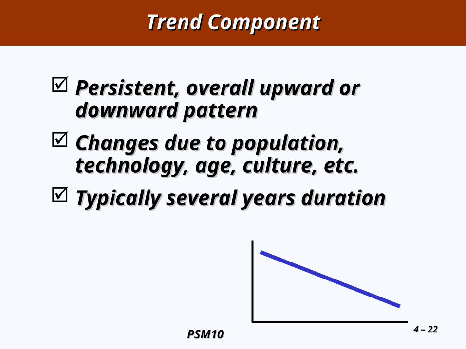
Trend ComponentTrend Component
Persistent, overall upward or Persistent, overall upward or downward patterndownward pattern
Changes due to population, Changes due to population, technology, age, culture, etc.technology, age, culture, etc.
Typically several years Typically several years duration duration

4 4 –– 2323PSM10PSM10
Seasonal ComponentSeasonal Component
Regular pattern of up and Regular pattern of up and down fluctuationsdown fluctuations
Due to weather, customs, etc.Due to weather, customs, etc.
Occurs within a single year Occurs within a single year
Number ofPeriod Length Seasons
Week Day 7Month Week 4-4.5Month Day 28-31Year Quarter 4Year Month 12Year Week 52

4 4 –– 2424PSM10PSM10
Cyclical ComponentCyclical Component
Repeating up and down movementsRepeating up and down movements
Affected by business cycle, political, Affected by business cycle, political, and economic factorsand economic factors
Multiple years durationMultiple years duration
Often causal or Often causal or associative associative relationshipsrelationships
00 55 1010 1515 2020

4 4 –– 2525PSM10PSM10
Random ComponentRandom Component
Erratic, unsystematic, ‘residual’ Erratic, unsystematic, ‘residual’ fluctuationsfluctuations
Due to random variation or Due to random variation or unforeseen eventsunforeseen events
Short duration and Short duration and nonrepeating nonrepeating
MM TT WW TT FF
4 4 –– 2626PSM10PSM10
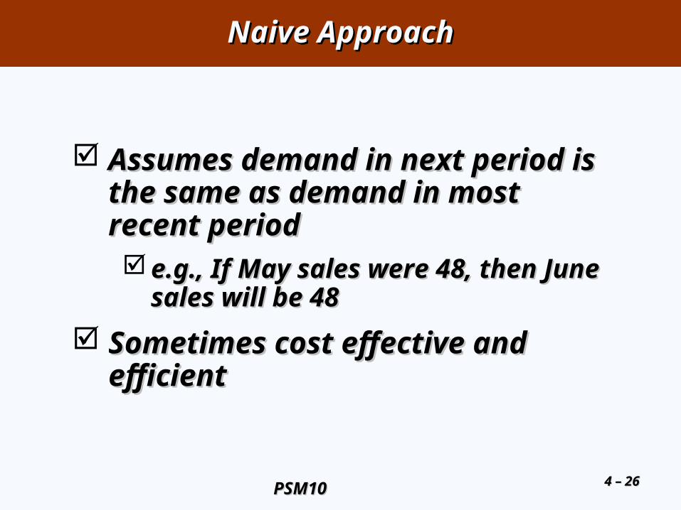
Naive ApproachNaive Approach
Assumes demand in next period is Assumes demand in next period is the same as demand in most the same as demand in most recent periodrecent period e.g., If May sales were 48, then June e.g., If May sales were 48, then June
sales will be 48sales will be 48
Sometimes cost effective and Sometimes cost effective and efficientefficient

4 4 –– 2727PSM10PSM10
Moving Average MethodMoving Average Method
MA is a series of arithmetic means MA is a series of arithmetic means
Used if little or no trendUsed if little or no trend
Used often for smoothingUsed often for smoothingProvides overall impression of data Provides overall impression of data
over timeover time
Moving average =Moving average =∑∑ demand in previous n periodsdemand in previous n periods
nn

4 4 –– 2828PSM10PSM10
JanuaryJanuary 1010FebruaryFebruary 1212MarchMarch 1313AprilApril 1616MayMay 1919JuneJune 2323JulyJuly 2626
ActualActual 3-Month3-MonthMonthMonth Shed SalesShed Sales Moving AverageMoving Average
(12 + 13 + 16)/3 = 13 (12 + 13 + 16)/3 = 13 22//33
(13 + 16 + 19)/3 = 16(13 + 16 + 19)/3 = 16(16 + 19 + 23)/3 = 19 (16 + 19 + 23)/3 = 19 11//33
Moving Average ExampleMoving Average Example
101012121313
((1010 + + 1212 + + 1313)/3 = 11 )/3 = 11 22//33

4 4 –– 2929PSM10PSM10
Graph of Moving AverageGraph of Moving Average
| | | | | | | | | | | |
JJ FF MM AA MM JJ JJ AA SS OO NN DD
Sh
ed S
ales
Sh
ed S
ales
30 30 –28 28 –26 26 –24 24 –22 22 –20 20 –18 18 –16 16 –14 14 –12 12 –10 10 –
Actual Actual SalesSales
Moving Moving Average Average ForecastForecast

4 4 –– 3030PSM10PSM10
Weighted Moving AverageWeighted Moving Average
Used when trend is present Used when trend is present Older data usually less importantOlder data usually less important
Weights based on experience and Weights based on experience and intuitionintuition
WeightedWeightedmoving averagemoving average ==
∑∑ ((weight for period nweight for period n)) x x ((demand in period ndemand in period n))
∑∑ weightsweights

4 4 –– 3131PSM10PSM10
JanuaryJanuary 1010FebruaryFebruary 1212MarchMarch 1313AprilApril 1616MayMay 1919JuneJune 2323JulyJuly 2626
ActualActual 3-Month Weighted3-Month WeightedMonthMonth Shed SalesShed Sales Moving AverageMoving Average
[(3 x 16) + (2 x 13) + (12)]/6 = 14[(3 x 16) + (2 x 13) + (12)]/6 = 1411//33
[(3 x 19) + (2 x 16) + (13)]/6 = 17[(3 x 19) + (2 x 16) + (13)]/6 = 17[(3 x 23) + (2 x 19) + (16)]/6 = 20[(3 x 23) + (2 x 19) + (16)]/6 = 2011//22
Weighted Moving AverageWeighted Moving Average
101012121313
[(3 x [(3 x 1313) + (2 x ) + (2 x 1212) + () + (1010)]/6 = 12)]/6 = 1211//66
Weights Applied Period
3 Last month2 Two months ago1 Three months ago6 Sum of weights

4 4 –– 3232PSM10PSM10
Potential Problems With Moving AveragePotential Problems With Moving Average
Increasing n smooths the forecast Increasing n smooths the forecast but makes it less sensitive to but makes it less sensitive to changeschanges
Do not forecast trends wellDo not forecast trends well
Require extensive historical dataRequire extensive historical data

4 4 –– 3333PSM10PSM10
Moving Average And Weighted Moving Moving Average And Weighted Moving AverageAverage
30 30 –
25 25 –
20 20 –
15 15 –
10 10 –
5 5 –
Sa
les
de
man
dS
ale
s d
em
and
| | | | | | | | | | | |
JJ FF MM AA MM JJ JJ AA SS OO NN DD
Actual Actual salessales
Moving Moving averageaverage
Weighted Weighted moving moving averageaverage

4 4 –– 3434PSM10PSM10
Exponential SmoothingExponential Smoothing
Form of weighted moving averageForm of weighted moving average Weights decline exponentiallyWeights decline exponentially
Most recent data weighted mostMost recent data weighted most
Requires smoothing constant Requires smoothing constant (()) Ranges from 0 to 1Ranges from 0 to 1
Subjectively chosenSubjectively chosen
Involves little record keeping of past Involves little record keeping of past datadata

4 4 –– 3535PSM10PSM10
Exponential SmoothingExponential Smoothing
New forecast =New forecast = last period’s forecastlast period’s forecast+ + ((last period’s actual demand last period’s actual demand
– – last period’s forecastlast period’s forecast))
FFtt = F = Ft t – 1– 1 + + ((AAt t – 1– 1 - - F Ft t – 1– 1))
wherewhere FFtt == new forecastnew forecast
FFt t – 1– 1 == previous forecastprevious forecast
== smoothing (or weighting) smoothing (or weighting) constant constant (0 (0 1) 1)

4 4 –– 3636PSM10PSM10
Exponential Smoothing ExampleExponential Smoothing Example
Predicted demand Predicted demand = 142= 142 Ford Mustangs Ford MustangsActual demand Actual demand = 153= 153Smoothing constant Smoothing constant = .20 = .20

4 4 –– 3737PSM10PSM10
Exponential Smoothing ExampleExponential Smoothing Example
Predicted demand Predicted demand = 142= 142 Ford Mustangs Ford MustangsActual demand Actual demand = 153= 153Smoothing constant Smoothing constant = .20 = .20
New forecastNew forecast = 142 + .2(153 – 142)= 142 + .2(153 – 142)

4 4 –– 3838PSM10PSM10
Exponential Smoothing ExampleExponential Smoothing Example
Predicted demand Predicted demand = 142= 142 Ford Mustangs Ford MustangsActual demand Actual demand = 153= 153Smoothing constant Smoothing constant = .20 = .20
New forecastNew forecast = 142 + .2(153 – 142)= 142 + .2(153 – 142)
= 142 + 2.2= 142 + 2.2
= 144.2 ≈ 144 cars= 144.2 ≈ 144 cars

4 4 –– 3939PSM10PSM10
Effect ofEffect of Smoothing Constants Smoothing Constants
Weight Assigned toWeight Assigned to
MostMost 2nd Most2nd Most 3rd Most3rd Most 4th Most4th Most 5th Most5th MostRecentRecent RecentRecent RecentRecent RecentRecent RecentRecent
SmoothingSmoothing PeriodPeriod PeriodPeriod PeriodPeriod PeriodPeriod PeriodPeriodConstantConstant (()) (1 - (1 - )) (1 - (1 - ))22 (1 - (1 - ))33 (1 - (1 - ))44
= .1= .1 .1.1 .09.09 .081.081 .073.073 .066.066
= .5= .5 .5.5 .25.25 .125.125 .063.063 .031.031

4 4 –– 4040PSM10PSM10
Impact of Different Impact of Different
225 225 –
200 200 –
175 175 –
150 150 –| | | | | | | | |
11 22 33 44 55 66 77 88 99
QuarterQuarter
De
ma
nd
De
ma
nd
= .1= .1
Actual Actual demanddemand
= .5= .5

4 4 –– 4141PSM10PSM10
Choosing Choosing
The objective is to obtain the most The objective is to obtain the most accurate forecast no matter the accurate forecast no matter the techniquetechnique
We generally do this by selecting the We generally do this by selecting the model that gives us the lowest forecast model that gives us the lowest forecast errorerror
Forecast errorForecast error = Actual demand - Forecast value= Actual demand - Forecast value
= A= Att - F - Ftt

4 4 –– 4242PSM10PSM10
Other interpretationOther interpretation
FFtt = F = Ft t – 1– 1 + + ((AAt t - - F Ft t – 1– 1) – ) – forecast for the t+1st period, Aforecast for the t+1st period, At t – demand – demand
of the t-th period of the t-th period
11 ttt F)(AF 21 11 ttt F)(A)(A
22
1 11 ttt F)(A)(A
322
1 111 tttt F)(Ar)(A)(A
...F)(A)(A)(A tttt 33
22
1 111
iti
iAαα
01
Exponential smoothing is the weighted average of the Exponential smoothing is the weighted average of the complete historic demand. The weights are decreasing complete historic demand. The weights are decreasing exponentially from period to period.exponentially from period to period.

4 4 –– 4343PSM10PSM10
Common Measures of ErrorCommon Measures of Error
Mean Absolute Deviation Mean Absolute Deviation ((MADMAD))
MAD =MAD =∑∑ |actual - forecast||actual - forecast|
nn
Mean Squared Error Mean Squared Error ((MSEMSE))
MSE =MSE =∑∑ ((forecast errorsforecast errors))22
nn

4 4 –– 4444PSM10PSM10
Common Measures of ErrorCommon Measures of Error
Mean Absolute Percent Error Mean Absolute Percent Error ((MAPEMAPE))
MAPE =MAPE =100 100 ∑∑ |actual |actualii - forecast - forecastii|/actual|/actualii
nn
nn
i i = 1= 1

4 4 –– 4545PSM10PSM10
Comparison of Forecast Error Comparison of Forecast Error
RoundedRounded AbsoluteAbsolute RoundedRounded AbsoluteAbsoluteActualActual ForecastForecast DeviationDeviation ForecastForecast DeviationDeviation
TonnageTonnage withwith forfor withwith forforQuarterQuarter UnloadedUnloaded = .10 = .10 = .10 = .10 = .50 = .50 = .50 = .50
11 180180 175175 55 175175 5522 168168 176176 88 178178 101033 159159 175175 1616 173173 141444 175175 173173 22 166166 9955 190190 173173 1717 170170 202066 205205 175175 3030 180180 252577 180180 178178 22 193193 131388 182182 178178 44 186186 44
8484 100100

4 4 –– 4646PSM10PSM10
Comparison of Forecast Error Comparison of Forecast Error
RoundedRounded AbsoluteAbsolute RoundedRounded AbsoluteAbsoluteActualActual ForecastForecast DeviationDeviation ForecastForecast DeviationDeviationTonageTonage withwith forfor withwith forfor
QuarterQuarter UnloadedUnloaded = .10 = .10 = .10 = .10 = .50 = .50 = .50 = .50
11 180180 175175 55 175175 5522 168168 176176 88 178178 101033 159159 175175 1616 173173 141444 175175 173173 22 166166 9955 190190 173173 1717 170170 202066 205205 175175 3030 180180 252577 180180 178178 22 193193 131388 182182 178178 44 186186 44
8484 100100
MAD =∑ |deviations|
n
= 84/8 = 10.50
For = .10
= 100/8 = 12.50
For = .50

4 4 –– 4747PSM10PSM10
Comparison of Forecast Error Comparison of Forecast Error
RoundedRounded AbsoluteAbsolute RoundedRounded AbsoluteAbsoluteActualActual ForecastForecast DeviationDeviation ForecastForecast DeviationDeviationTonageTonage withwith forfor withwith forfor
QuarterQuarter UnloadedUnloaded = .10 = .10 = .10 = .10 = .50 = .50 = .50 = .50
11 180180 175175 55 175175 5522 168168 176176 88 178178 101033 159159 175175 1616 173173 141444 175175 173173 22 166166 9955 190190 173173 1717 170170 202066 205205 175175 3030 180180 252577 180180 178178 22 193193 131388 182182 178178 44 186186 44
8484 100100MADMAD 10.5010.50 12.5012.50
= 1,558/8 = 194.75
For = .10
= 1,612/8 = 201.50
For = .50
MSE =∑ (forecast errors)2
n

4 4 –– 4848PSM10PSM10
Comparison of Forecast Error Comparison of Forecast Error
RoundedRounded AbsoluteAbsolute RoundedRounded AbsoluteAbsoluteActualActual ForecastForecast DeviationDeviation ForecastForecast DeviationDeviationTonageTonage withwith forfor withwith forfor
QuarterQuarter UnloadedUnloaded = .10 = .10 = .10 = .10 = .50 = .50 = .50 = .50
11 180180 175175 55 175175 5522 168168 176176 88 178178 101033 159159 175175 1616 173173 141444 175175 173173 22 166166 9955 190190 173173 1717 170170 202066 205205 175175 3030 180180 252577 180180 178178 22 193193 131388 182182 178178 44 186186 44
8484 100100MADMAD 10.5010.50 12.5012.50MSEMSE 194.75194.75 201.50201.50
= 45.62/8 = 5.70%
For = .10
= 54.8/8 = 6.85%
For = .50
MAPE =100 ∑ |deviationi|/actuali
n
n
i = 1

4 4 –– 4949PSM10PSM10
Comparison of Forecast Error Comparison of Forecast Error
RoundedRounded AbsoluteAbsolute RoundedRounded AbsoluteAbsoluteActualActual ForecastForecast DeviationDeviation ForecastForecast DeviationDeviation
TonnageTonnage withwith forfor withwith forforQuarterQuarter UnloadedUnloaded = .10 = .10 = .10 = .10 = .50 = .50 = .50 = .50
11 180180 175175 55 175175 5522 168168 176176 88 178178 101033 159159 175175 1616 173173 141444 175175 173173 22 166166 9955 190190 173173 1717 170170 202066 205205 175175 3030 180180 252577 180180 178178 22 193193 131388 182182 178178 44 186186 44
8484 100100MADMAD 10.5010.50 12.5012.50MSEMSE 194.75194.75 201.50201.50
MAPEMAPE 5.70%5.70% 6.85%6.85%

4 4 –– 5050PSM10PSM10
Exponential Smoothing with Trend Exponential Smoothing with Trend AdjustmentAdjustment
When a trend is present, exponential When a trend is present, exponential smoothing must be modifiedsmoothing must be modified
Forecast Forecast including including ((FITFITtt)) = = trendtrend
exponentiallyexponentially exponentiallyexponentiallysmoothed smoothed ((FFtt)) + + ((TTtt)) smoothedsmoothedforecastforecast trendtrend

4 4 –– 5151PSM10PSM10
Exponential Smoothing with Trend Exponential Smoothing with Trend AdjustmentAdjustment
Step 1: Compute FStep 1: Compute Ftt
Step 2: Compute TStep 2: Compute Ttt
Step 3: Calculate the forecast FITStep 3: Calculate the forecast FITtt == F Ftt + + TTtt
11
111
1
1
tttt
tttt
TFFT
TFAF

4 4 –– 5252PSM10PSM10
Exponential Smoothing with Trend Exponential Smoothing with Trend Adjustment ExampleAdjustment Example
ForecastForecastActualActual SmoothedSmoothed SmoothedSmoothed IncludingIncluding
MonthMonth((tt)) Demand Demand ((AAtt)) Forecast, FForecast, Ftt Trend, TTrend, Ttt Trend, FITTrend, FITtt
11 1212 1111 22 13.0013.0022 171733 202044 191955 242466 212177 313188 282899 3636
1010

4 4 –– 5353PSM10PSM10
Exponential Smoothing with Trend Exponential Smoothing with Trend Adjustment ExampleAdjustment Example
ForecastForecastActualActual SmoothedSmoothed SmoothedSmoothed IncludingIncluding
MonthMonth((tt)) Demand Demand ((AAtt)) Forecast, FForecast, Ftt Trend, TTrend, Ttt Trend, FITTrend, FITtt
11 1212 1111 22 13.0013.0022 171733 202044 191955 242466 212177 313188 282899 3636
1010
F2 = A1 + (1 - )(F1 + T1)
F2 = (.2)(12) + (1 - .2)(11 + 2)
= 2.4 + 10.4 = 12.8 units
Step 1: Forecast for Month 2

4 4 –– 5454PSM10PSM10
Exponential Smoothing with Trend Exponential Smoothing with Trend Adjustment ExampleAdjustment Example
ForecastForecastActualActual SmoothedSmoothed SmoothedSmoothed IncludingIncluding
MonthMonth((tt)) Demand Demand ((AAtt)) Forecast, FForecast, Ftt Trend, TTrend, Ttt Trend, FITTrend, FITtt
11 1212 1111 22 13.0013.0022 1717 12.8012.8033 202044 191955 242466 212177 313188 282899 3636
1010
T2 = (F2 - F1) + (1 - )T1
T2 = (.4)(12.8 - 11) + (1 - .4)(2)
= .72 + 1.2 = 1.92 units
Step 2: Trend for Month 2

4 4 –– 5555PSM10PSM10
Exponential Smoothing with Trend Exponential Smoothing with Trend Adjustment ExampleAdjustment Example
ForecastForecastActualActual SmoothedSmoothed SmoothedSmoothed IncludingIncluding
MonthMonth((tt)) Demand Demand ((AAtt)) Forecast, FForecast, Ftt Trend, TTrend, Ttt Trend, FITTrend, FITtt
11 1212 1111 22 13.0013.0022 1717 12.8012.80 1.921.9233 202044 191955 242466 212177 313188 282899 3636
1010
FIT2 = F2 + T1
FIT2 = 12.8 + 1.92
= 14.72 units
Step 3: Calculate FIT for Month 2
4 4 –– 5656PSM10PSM10
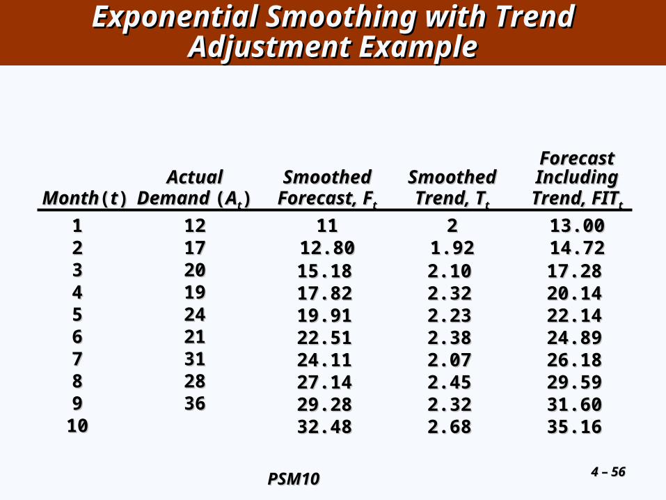
Exponential Smoothing with Trend Exponential Smoothing with Trend Adjustment ExampleAdjustment Example
ForecastForecastActualActual SmoothedSmoothed SmoothedSmoothed IncludingIncluding
MonthMonth((tt)) Demand Demand ((AAtt)) Forecast, FForecast, Ftt Trend, TTrend, Ttt Trend, FITTrend, FITtt
11 1212 1111 22 13.0013.0022 1717 12.8012.80 1.921.92 14.7214.7233 202044 191955 242466 212177 313188 282899 3636
1010
15.1815.18 2.102.10 17.2817.2817.8217.82 2.322.32 20.1420.1419.9119.91 2.232.23 22.1422.1422.5122.51 2.382.38 24.8924.8924.1124.11 2.072.07 26.1826.1827.1427.14 2.452.45 29.5929.5929.2829.28 2.322.32 31.6031.6032.4832.48 2.682.68 35.1635.16

4 4 –– 5757PSM10PSM10
Exponential Smoothing with Trend Exponential Smoothing with Trend Adjustment ExampleAdjustment Example
| | | | | | | | |
11 22 33 44 55 66 77 88 99
Time (month)Time (month)
Pro
du
ct d
eman
dP
rod
uct
dem
and
35 35 –
30 30 –
25 25 –
20 20 –
15 15 –
10 10 –
5 5 –
0 0 –
Actual demand Actual demand ((AAtt))
Forecast including trend Forecast including trend ((FITFITtt))

4 4 –– 5858PSM10PSM10
Trend ProjectionsTrend Projections
Fitting a trend line to historical data points Fitting a trend line to historical data points to project into the medium-to-long-rangeto project into the medium-to-long-range
Linear trends can be found using the least Linear trends can be found using the least squares technique (regression analysis)squares technique (regression analysis)
y y = = a a + + bxbx^̂
where ywhere y= computed value of the = computed value of the variable to be predicted (dependent variable to be predicted (dependent variable)variable)aa= y-axis intercept= y-axis interceptbb= slope of the regression line= slope of the regression linexx= the independent variable= the independent variable
^̂

4 4 –– 5959PSM10PSM10
Least Squares MethodLeast Squares Method
Time periodTime period
Va
lue
s o
f D
ep
end
en
t V
ari
able
DeviationDeviation11
DeviationDeviation55
DeviationDeviation77
DeviationDeviation22
DeviationDeviation66
DeviationDeviation44
DeviationDeviation33
Actual observation Actual observation (y value)(y value)
Trend line, y = a + bxTrend line, y = a + bx^̂

4 4 –– 6060PSM10PSM10
Least Squares MethodLeast Squares Method
Time periodTime period
Va
lue
s o
f D
ep
end
en
t V
ari
able
DeviationDeviation11
DeviationDeviation55
DeviationDeviation77
DeviationDeviation22
DeviationDeviation66
DeviationDeviation44
DeviationDeviation33
Actual observation Actual observation (y value)(y value)
Trend line, y = a + bxTrend line, y = a + bx^̂
Least squares method minimizes the sum of the
squared errors (deviations)
4 4 –– 6161PSM10PSM10
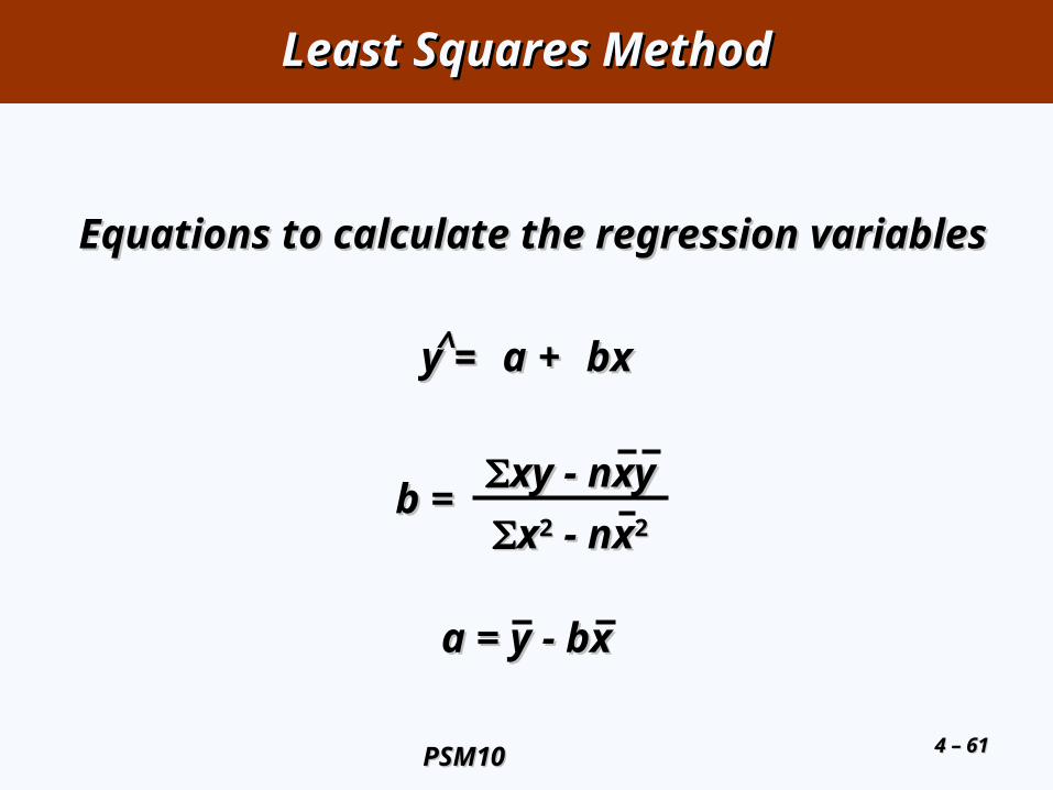
Least Squares MethodLeast Squares Method
Equations to calculate the regression variablesEquations to calculate the regression variables
b =b =xy - nxyxy - nxy
xx22 - nx - nx22
y y = = a a + + bxbx^̂
a = y - bxa = y - bx

4 4 –– 6262PSM10PSM10
Least Squares ExampleLeast Squares Example
b b = = = 10.54= = = 10.54∑∑xy - nxyxy - nxy
∑∑xx22 - nx - nx22
3,063 - (7)(4)(98.86)3,063 - (7)(4)(98.86)
140 - (7)(4140 - (7)(422))
aa = = yy - - bxbx = 98.86 - 10.54(4) = 56.70 = 98.86 - 10.54(4) = 56.70
TimeTime Electrical Power Electrical Power YearYear Period (x)Period (x) DemandDemand xx22 xyxy
19991999 11 7474 11 747420002000 22 7979 44 15815820012001 33 8080 99 24024020022002 44 9090 1616 36036020032003 55 105105 2525 52552520042004 66 142142 3636 85285220052005 77 122122 4949 854854
∑∑xx = 28 = 28 ∑∑yy = 692 = 692 ∑∑xx22 = 140 = 140 ∑∑xyxy = 3,063 = 3,063xx = 4 = 4 yy = 98.86 = 98.86

4 4 –– 6363PSM10PSM10
Least Squares ExampleLeast Squares Example
b b = = = 10.54= = = 10.54xy - nxyxy - nxy
xx22 - nx - nx22
3,063 - (7)(4)(98.86)3,063 - (7)(4)(98.86)
140 - (7)(4140 - (7)(422))
aa = = yy - - bxbx = 98.86 - 10.54(4) = 56.70 = 98.86 - 10.54(4) = 56.70
TimeTime Electrical Power Electrical Power YearYear Period (x)Period (x) DemandDemand xx22 xyxy
19991999 11 7474 11 747420002000 22 7979 44 15815820012001 33 8080 99 24024020022002 44 9090 1616 36036020032003 55 105105 2525 52552520042004 66 142142 3636 85285220052005 77 122122 4949 854854
xx = 28 = 28 yy = 692 = 692 xx22 = 140 = 140 xyxy = 3,063 = 3,063xx = 4 = 4 yy = 98.86 = 98.86
The trend line is
y = 56.70 + 10.54x^

4 4 –– 6464PSM10PSM10
Least Squares ExampleLeast Squares Example
| | | | | | | | |19991999 20002000 20012001 20022002 20032003 20042004 20052005 20062006 20072007
160 160 –
150 150 –
140 140 –
130 130 –
120 120 –
110 110 –
100 100 –
90 90 –
80 80 –
70 70 –
60 60 –
50 50 –
YearYear
Po
wer
dem
and
Po
wer
dem
and
Trend line,Trend line,y y = 56.70 + 10.54x= 56.70 + 10.54x^̂
141=141=56.7+8*10.5456.7+8*10.54
4 4 –– 6666PSM10PSM10
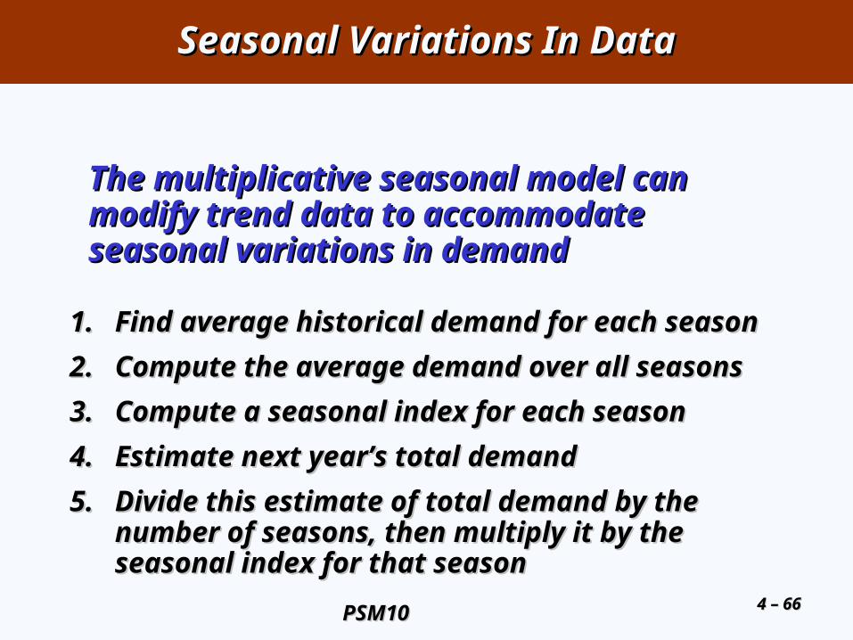
Seasonal Variations In DataSeasonal Variations In Data
The multiplicative seasonal model can The multiplicative seasonal model can modify trend data to accommodate modify trend data to accommodate seasonal variations in demandseasonal variations in demand
1.1. Find average historical demand for each season Find average historical demand for each season
2.2. Compute the average demand over all seasons Compute the average demand over all seasons
3.3. Compute a seasonal index for each season Compute a seasonal index for each season
4.4. Estimate next year’s total demandEstimate next year’s total demand
5.5. Divide this estimate of total demand by the Divide this estimate of total demand by the number of seasons, then multiply it by the number of seasons, then multiply it by the seasonal index for that seasonseasonal index for that season

4 4 –– 6767PSM10PSM10
Seasonal Index ExampleSeasonal Index Example
JanJan 8080 8585 105105 9090 9494
FebFeb 7070 8585 8585 8080 9494
MarMar 8080 9393 8282 8585 9494
AprApr 9090 9595 115115 100100 9494
MayMay 113113 125125 131131 123123 9494
JunJun 110110 115115 120120 115115 9494
JulJul 100100 102102 113113 105105 9494
AugAug 8888 102102 110110 100100 9494
SeptSept 8585 9090 9595 9090 9494
OctOct 7777 7878 8585 8080 9494
NovNov 7575 7272 8383 8080 9494
DecDec 8282 7878 8080 8080 9494
DemandDemand AverageAverage AverageAverage Seasonal Seasonal MonthMonth 20032003 20042004 20052005 2003-20052003-2005 MonthlyMonthly IndexIndex

4 4 –– 6868PSM10PSM10
Seasonal Index ExampleSeasonal Index Example
JanJan 8080 8585 105105 9090 9494
FebFeb 7070 8585 8585 8080 9494
MarMar 8080 9393 8282 8585 9494
AprApr 9090 9595 115115 100100 9494
MayMay 113113 125125 131131 123123 9494
JunJun 110110 115115 120120 115115 9494
JulJul 100100 102102 113113 105105 9494
AugAug 8888 102102 110110 100100 9494
SeptSept 8585 9090 9595 9090 9494
OctOct 7777 7878 8585 8080 9494
NovNov 7575 7272 8383 8080 9494
DecDec 8282 7878 8080 8080 9494
DemandDemand AverageAverage AverageAverage Seasonal Seasonal MonthMonth 20032003 20042004 20052005 2003-20052003-2005 MonthlyMonthly IndexIndex
0.9570.957
Seasonal index = average 2003-2005 monthly demand
average monthly demand
= 90/94 = .957

4 4 –– 6969PSM10PSM10
Seasonal Index ExampleSeasonal Index Example
JanJan 8080 8585 105105 9090 9494 0.9570.957
FebFeb 7070 8585 8585 8080 9494 0.8510.851
MarMar 8080 9393 8282 8585 9494 0.9040.904
AprApr 9090 9595 115115 100100 9494 1.0641.064
MayMay 113113 125125 131131 123123 9494 1.3091.309
JunJun 110110 115115 120120 115115 9494 1.2231.223
JulJul 100100 102102 113113 105105 9494 1.1171.117
AugAug 8888 102102 110110 100100 9494 1.0641.064
SeptSept 8585 9090 9595 9090 9494 0.9570.957
OctOct 7777 7878 8585 8080 9494 0.8510.851
NovNov 7575 7272 8383 8080 9494 0.8510.851
DecDec 8282 7878 8080 8080 9494 0.8510.851
DemandDemand AverageAverage AverageAverage Seasonal Seasonal MonthMonth 20032003 20042004 20052005 2003-20052003-2005 MonthlyMonthly IndexIndex
1,1281,128

4 4 –– 7070PSM10PSM10
Seasonal Index ExampleSeasonal Index Example
JanJan 8080 8585 105105 9090 9494 0.9570.957
FebFeb 7070 8585 8585 8080 9494 0.8510.851
MarMar 8080 9393 8282 8585 9494 0.9040.904
AprApr 9090 9595 115115 100100 9494 1.0641.064
MayMay 113113 125125 131131 123123 9494 1.3091.309
JunJun 110110 115115 120120 115115 9494 1.2231.223
JulJul 100100 102102 113113 105105 9494 1.1171.117
AugAug 8888 102102 110110 100100 9494 1.0641.064
SeptSept 8585 9090 9595 9090 9494 0.9570.957
OctOct 7777 7878 8585 8080 9494 0.8510.851
NovNov 7575 7272 8383 8080 9494 0.8510.851
DecDec 8282 7878 8080 8080 9494 0.8510.851
DemandDemand AverageAverage AverageAverage Seasonal Seasonal MonthMonth 20032003 20042004 20052005 2003-20052003-2005 MonthlyMonthly IndexIndex
Expected annual demand = 1,200
Jan x .957 = 961,200
12
Feb x .851 = 851,200
12
Forecast for 2006

4 4 –– 7171PSM10PSM10
Seasonal Index ExampleSeasonal Index Example
JanJan 95,70
FebFeb 85,10
MarMar 90,40
AprApr 106,40
MayMay 130,90
JunJun 122,30
JulJul 111,70
AugAug 106,40
SeptSept 95,70
OctOct 85,10
NovNov 85,10
DecDec 85,10
60,00
80,00
100,00
120,00
140,00
1 2 3 4 5 6 7 8 9 10 11 12

4 4 –– 7272PSM10PSM10
Seasonal Index ExampleSeasonal Index Example
140 140 –
130 130 –
120 120 –
110 110 –
100 100 –
90 90 –
80 80 –
70 70 –| | | | | | | | | | | |
JJ FF MM AA MM JJ JJ AA SS OO NN DD
TimeTime
Dem
and
Dem
and
2006 Forecast2006 Forecast
2005 Demand 2005 Demand
2004 Demand2004 Demand
2003 Demand2003 Demand

4 4 –– 7373PSM10PSM10
Monitoring and Controlling ForecastsMonitoring and Controlling Forecasts
Measures how well the forecast is Measures how well the forecast is predicting actual valuespredicting actual values
Ratio of running sum of forecast errors Ratio of running sum of forecast errors (RSFE) to mean absolute deviation (MAD)(RSFE) to mean absolute deviation (MAD) Good tracking signal has low valuesGood tracking signal has low values
If forecasts are continually high or low, the If forecasts are continually high or low, the forecast has a bias errorforecast has a bias error
Tracking SignalTracking Signal

4 4 –– 7474PSM10PSM10
Monitoring and Controlling ForecastsMonitoring and Controlling Forecasts
Tracking Tracking signalsignal
RSFERSFEMADMAD==
Tracking Tracking signalsignal ==
∑∑(actual demand in (actual demand in period i - period i -
forecast demand forecast demand in period i)in period i)
∑∑|actual - forecast|/n|actual - forecast|/n))

4 4 –– 7575PSM10PSM10
Tracking SignalTracking Signal
Tracking signalTracking signal
++
00 MADs MADs
––
Upper control limitUpper control limit
Lower control limitLower control limit
TimeTime
Signal exceeding limitSignal exceeding limit
Acceptable Acceptable rangerange

4 4 –– 7676PSM10PSM10
Tracking Signal ExampleTracking Signal Example
CumulativeCumulativeAbsoluteAbsolute AbsoluteAbsolute
ActualActual ForecastForecast ForecastForecast ForecastForecastQtrQtr DemandDemand DemandDemand ErrorError RSFERSFE ErrorError ErrorError MADMAD
11 9090 100100 -10-10 -10-10 1010 1010 10.010.022 9595 100100 -5-5 -15-15 55 1515 7.57.533 115115 100100 +15+15 00 1515 3030 10.010.044 100100 110110 -10-10 -10-10 1010 4040 10.010.055 125125 110110 +15+15 +5+5 1515 5555 11.011.066 140140 110110 +30+30 +35+35 3030 8585 14.214.2

4 4 –– 7777PSM10PSM10
CumulativeCumulativeAbsoluteAbsolute AbsoluteAbsolute
ActualActual ForecastForecast ForecastForecast ForecastForecastQtrQtr DemandDemand DemandDemand ErrorError RSFERSFE ErrorError ErrorError MADMAD
11 9090 100100 -10-10 -10-10 1010 1010 10.010.022 9595 100100 -5-5 -15-15 55 1515 7.57.533 115115 100100 +15+15 00 1515 3030 10.010.044 100100 110110 -10-10 -10-10 1010 4040 10.010.055 125125 110110 +15+15 +5+5 1515 5555 11.011.066 140140 110110 +30+30 +35+35 3030 8585 14.214.2
Tracking Signal ExampleTracking Signal Example
TrackingSignal
(RSFE/MAD)
-10/10 = -1-15/7.5 = -2
0/10 = 0-10/10 = -1
+5/11 = +0.5+35/14.2 = +2.5
The variation of the tracking signal The variation of the tracking signal between between -2.0-2.0 and and +2.5+2.5 is within acceptable is within acceptable limitslimits

4 4 –– 7878PSM10PSM10
Forecasting in the Service SectorForecasting in the Service Sector
Presents unusual challengesPresents unusual challenges Special need for short term recordsSpecial need for short term records
Needs differ greatly as function of Needs differ greatly as function of industry and productindustry and product
Holidays and other calendar eventsHolidays and other calendar events
Unusual eventsUnusual events

4 4 –– 7979PSM10PSM10
QuestionsQuestions
Answer the following questionsAnswer the following questions
How would you rate the time horizon for long range forecast in the field of How would you rate the time horizon for long range forecast in the field of mobile information technologies? mobile information technologies?
Which of the Seven Steps in Forecasting is the most interesting for you?Which of the Seven Steps in Forecasting is the most interesting for you?
Did you ever use the method of “Jury of Executive Opinion” when Did you ever use the method of “Jury of Executive Opinion” when discussing family affairs at home?discussing family affairs at home?
Which week sides if the Delphi method would you identify?Which week sides if the Delphi method would you identify?
Under which circumstances do the Weighted Moving Average method and Under which circumstances do the Weighted Moving Average method and the method of exponential smoothing coincide?the method of exponential smoothing coincide?
Can the two methods of exponential smoothing ever coincide?Can the two methods of exponential smoothing ever coincide?
Look for the various opportunities of using forecast methods by Excel.Look for the various opportunities of using forecast methods by Excel.
Let the demand follow the function d(t) = 10 + 2t and apply the simple Let the demand follow the function d(t) = 10 + 2t and apply the simple weighted average forecast method with n = 2. What can you say about the weighted average forecast method with n = 2. What can you say about the tracking signal?tracking signal?

4 4 –– 8080PSM10PSM10
QuestionsQuestions
Homework No. 3:Homework No. 3:
Create an Excel Spreadsheet to solve the following problem! Sales of music Create an Excel Spreadsheet to solve the following problem! Sales of music stands at Johnny Ho’s music store, in Columbus, Ohio, over the past 10 weeks stands at Johnny Ho’s music store, in Columbus, Ohio, over the past 10 weeks are shown in the table below. are shown in the table below.
WeekWeek DemandDemand WeekWeek DemandDemand
11 2020 66 2929
22 2121 77 3636
33 2828 88 2222
44 3737 99 2525
55 2525 1010 2?2?
a)a) Forecast demand for each week, including week 10, using exponential Forecast demand for each week, including week 10, using exponential smoothing with smoothing with αα = 0.3 (initial forecast F = 0.3 (initial forecast F11 = 20) = 20)
b)b) Compute the MADCompute the MAD..
c)c) Compute the tracking signal. Compute the tracking signal. Submit your solution file via E-Mail to Submit your solution file via E-Mail to [email protected] (term: 29.04.2010). (term: 29.04.2010).
Don’t forget to indicate your university ID card number. Don’t forget to indicate your university ID card number.
Put here the last digit of your Put here the last digit of your university ID card number. university ID card number.