A Review of Water Scarcity Indices and Methodologies

FOOD, BEVERAGE & AGRICULTURE

Amber BrownMarty D. Matlock, Ph.D., P.E., C.S.E.University of ArkansasThe Sustainability Consortium

White Paper #106 | April 2011

© 2011 The Sustainability Consortium

Page | i

TABLE OF CONTENTS

1. Introduction ................................................................................................................................... 1

2. Indices Based on Human Water Requirements ................................................................................ 1

2.1. The Falkenmark Indicator ................................................................................................................. 1

2.2. Basic Human Water Requirements ................................................................................................... 2

2.3. The Social Water Stress Index ........................................................................................................... 2

2.4. Water Resources Availability and Cereal Import ............................................................................. 3

3. Water Resources Vulnerability Indices ............................................................................................ 3

3.1. The Index of Local Relative Water Use and Reuse ........................................................................... 4

3.2. The Watershed Sustainability Index ................................................................................................. 5

3.3. The Water Supply Stress Index ......................................................................................................... 7

3.4. Physical and Economical Water Scarcity .......................................................................................... 8

4. Indices Incorporating Environmental Water Requirements .............................................................. 9

4.1. Population Growth Impacts on Water Resource Availability .......................................................... 9

4.2. Assessing Water Resource Supplies Using the Water Stress Indicator ......................................... 10

5. LCA and Water Footprint .............................................................................................................. 11

5.1. Life Cycle Assessment and WSI ....................................................................................................... 11

5.1.1. Methodology ............................................................................................................................. 12

5.1.2. Damage to Human Health, Ecosystem Quality, and Resources ............................................... 12

5.2. Water Footprinting.......................................................................................................................... 13

5.3. A Revised Approach to Water Footprinting ................................................................................... 13

Social impacts of green water use ...................................................................................................... 14

Social Impacts of blue water use ........................................................................................................ 14

Environmental impacts of green water use ........................................................................................ 15

Environmental impacts of blue water use .......................................................................................... 15

6. Conclusion ................................................................................................................................... 15

References ....................................................................................................................................... 17

Page | 1

1. Introduction In the past 20 years many indices have been developed to quantitatively evaluate water

resources vulnerability (e.g. water scarcity or water stress). The difficulty of characterizing

water stress is that there are many equally important facets to water use, supply and scarcity.

Selecting the criteria by which water is assessed can be as much a policy decision as a scientific

decision. This review provides an overview of the primary water scarcity indices and water

resource assessment methodologies at the forefront of political and corporate decision making.

2. Indices Based on Human Water Requirements Freshwater scarcity is commonly described as a function of available water resources and

human population. These figures are generally expressed in terms of annual per capita water and

mostly on a national scale. The logic behind their development is simply that if we know how

much water is necessary to meet human demands, then the water that is available to each person

can serve as a measure of scarcity (Rijsberman 2006).

2.1. The Falkenmark Indicator

The Falkenmark indicator is perhaps the most widely used measure of water stress. It is

defined as the fraction of the total annual runoff available for human use. Multiple countries

were surveyed and the water usage per person in each economy was calculated. Based on the per

capita usage, the water conditions in an area can be categorized as: no stress, stress, scarcity, and

absolute scarcity (Table 1). The index thresholds 1,700m3 and 1000m

3 per capita per year are

used as the thresholds between water stressed and scarce areas, respectively (Falkenmark 1989).

Table 1. Water barrier differentiation proposed by Falkenmark (1989)

Index

(m3 per capita)

Category/Condition

>1,700 No Stress

1,000-1,700 Stress

500-1,000 Scarcity

<500 Absolute Scarcity

Individual usage is the basis for the Falkenmark water stress index and therefore provides a

way of distinguishing between climate and human-induced water scarcity (Vorosmarty et al.,

2005). This index is typically used in assessments on a country scale where the data is readily

available and provides results that are intuitive and easy to understand. However, the use of

national annual averages tends to obscure important scarcity information at smaller scales.

Simple thresholds omit important variations in demand among countries due to culture, lifestyle,

Page | 2

climate, etc (Rijsberman 2006). Finally, this index appears to under-measure the impact of

smaller populations, by failing to measure water stress at these scales.

2.2. Basic Human Water Requirements

Gleick (1996) developed a water scarcity index as a measurement of the ability to meet all

water requirements for basic human needs: drinking water for survival, water for human hygiene,

water for sanitation services, and modest household needs for preparing food. The proposed

minimum amount needed to sustain each is as follows:

1. Minimum Drinking Water Requirement: Data from the National Research Council of the

National Academy of Sciences was used to estimate the minimum drinking water

requirement for human survival under typical temperate climates with normal activity is

about 5 liters per person per day.

2. Basic Requirements for Sanitation: Taking into account various technologies for

sanitation worldwide, the effective disposal of human wastes can be accomplished with

little to no water if necessary. However, to account for the maximum benefits of

combining waste disposal and related hygiene as well as to allow for cultural and societal

preferences, a minimum of 20 liters per person per day is recommended.

3. Basic Water Requirements for Bathing: Studies have suggested that the minimum amount

of water needed for adequate bathing is 15 liters per person per day (Kalbermatten et al.,

1982; Gleick 1993).

4. Basic Requirement for Food Preparation: Taking into consideration both developed and

underdeveloped countries, the water use for food preparation to satisfy most regional

standards and to meet basic needs is 10 liters per person per day.

The proposed water requirements for meeting basic human needs gives a total demand of 50

liters per person per day. International organizations and water providers are recommended to

adopt this overall basic water requirement as a new threshold for meeting these basic needs,

independent of climate, technology, and culture (P. H. Gleick 1996). Both Falkenmark and

Gleick developed the “benchmark indicator” of 1,000m3 per capita per year as a standard that has

been accepted by the World Bank (Gleick 1995; Falkenmark and Widstrand 1992).

2.3. The Social Water Stress Index Building on the Falkenmark indicator, Ohlsson (2000) integrated the “adaptive capacity” of a

society to consider how economic, technological, or other means affect the overall freshwater

availability status of a region. Ohlsson argued that the capability of a society to adapt to difficult

scenarios is a function of the distribution of wealth, education opportunities, and political

participation. The UNDP Human Development Index (HDI) is a widely accepted indicator used

to assess these societal variables. The HDI functions as a weighted measure of the Falkenmark

indicator in order to account for the ability to adapt to water stress and is termed the Social Water

Stress Index.

Page | 3

2.4. Water Resources Availability and Cereal Import Roughly 70% of the world‟s freshwater withdrawals are for agricultural use (FAO 2010).

Therefore, a relationship between available water resources and the ability to produce food

exists. Countries limited in available freshwater rely on importing food in order to compensate

for lack of production ability. The dominating food imported to most water scarce countries is

cereal grains (Yang and Zehnder 2002). Yang et al. (2003) suggest that with the strong

correlation between the volume of available freshwater resources and the quantity of imported

food, the development of a model to serve as a water-deficit indicator is possible. From such a

model, a threshold could be established that would provide a regional separation between water-

scarce and water-abundant statuses. Regions falling below this threshold would lack water

resources required for local food production, and cereal grains must be imported to compensate

for the water deficit.

Yearly average water data was used for each country representing a single unit due to the

availability of data being annual and country based, as well as the ease in the quantification of

water transfer across political boundaries. Africa and Asia were the two continents used in the

analysis since their combined annual imported net cereal grains amounted to over 110 million

tons in the 1990s, which would require all excess freshwater resources from all other continents.

These two regions are also home to a majority of the people living in food insecurity and

poverty. A water availability of 5000 m3/ (capita year) was used as the cutoff value to guarantee

that the water scarce countries were considered in the analysis while allowing for a comparison

with water-abundant countries. Furthermore, the countries analyzed were limited to those

exceeding 1 million inhabitants.

The authors found that in nearly all the countries that fell below the water-deficit threshold,

there was an increase in per capita cereal import. However, per capita import remained constant

in the countries above the threshold, suggesting no significant relationship between changes in

their per capita water resources and the volume of cereal import. There is also an inverse

relationship between availability of land resources and cereal import.

A threshold of 1,700 m3/ (capita year) suggested by Falkenmark falls within the calculated

threshold by Yang et al. (2003). However, the threshold calculated by this approach is dynamic

in that it can vary with irrigation practices or improvements in water use efficiency, whereas the

widely cited threshold developed by Falkenmark is a fixed value (Vorosmarty, et al., 2005). The

model developed by Yang et al. (2003) does not take in to account the use of non-renewable

groundwater due to the lack of systematic data. Thus the threshold values are somewhat

conservative.

3. Water Resources Vulnerability Indices The water scarcity indices thus far have measured water resource status based on fixed

human water requirements and water availability, mostly on a national scale but have not

Page | 4

incorporated renewable water supply and national, annual demand for water (Rijsberman 2006).

In 1987 Shiklomanov and Markova from the State Hydrological Institute in St. Petersburg

published estimated current and predicted water-resources use by region and sector

(Shiklomanov 1993). Water use was separated into industrial, agricultural, and domestic sectors,

as well as incorporated water lost from reservoir evaporation. Population and economic factors

were used as the major variables. Raskin et al. (1997) used Shiklomanov‟s water resource

availability data and modified the approach by substituting water withdrawals in place of water

demand. Since water demand varies between societies, cultures, and regions, the term is

subjective (Rijsberman 2006) and using it as a variable can lead to inaccurate assessments. The

Water Resources Vulnerability Index, sometimes referred to as the WTA ratio, was then

developed as the ratio of total annual withdrawals to available water resources. A country is then

considered water scarce if annual withdrawals are between 20 and 40% of annual supply, and

severely water scarce if withdrawals exceed 40% (Raskin, et al., 1997). This method and 40%

threshold is commonly used in water resources analyses and has been termed the “criticality

ratio”—the ratio of water withdrawals for human use to total renewable water resources

(Alcamo, Henrichs and Rosch 2000).

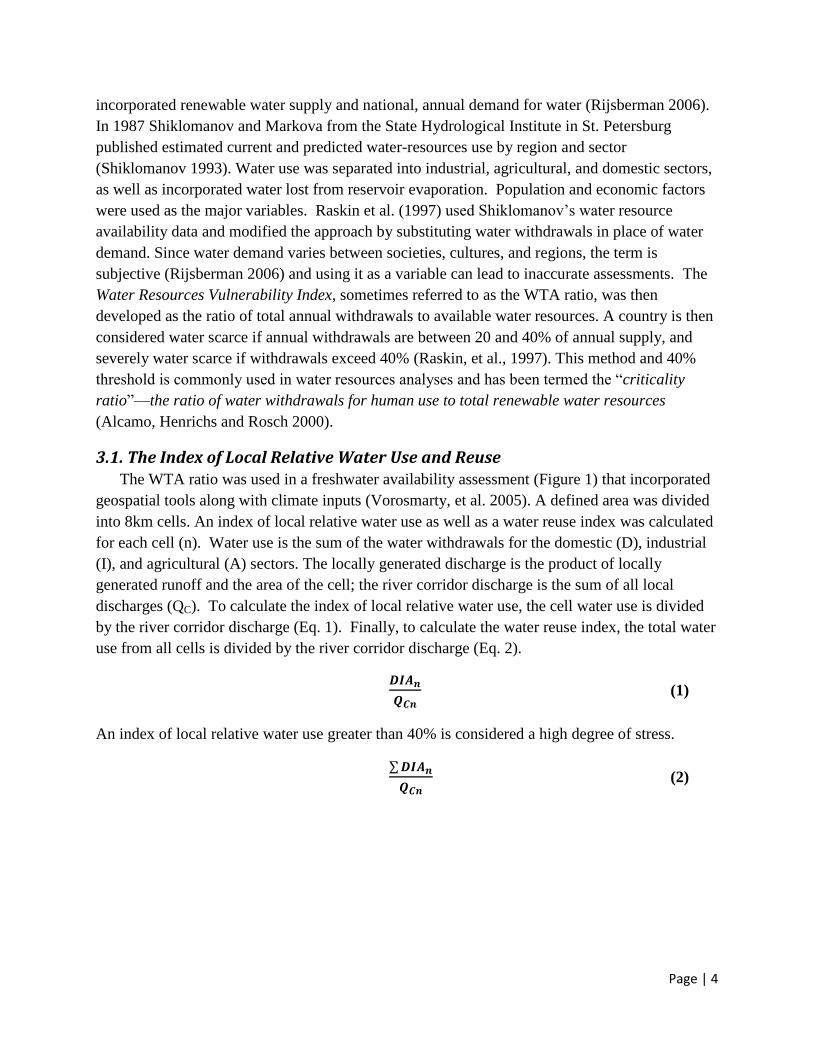
3.1. The Index of Local Relative Water Use and Reuse The WTA ratio was used in a freshwater availability assessment (Figure 1) that incorporated

geospatial tools along with climate inputs (Vorosmarty, et al. 2005). A defined area was divided

into 8km cells. An index of local relative water use as well as a water reuse index was calculated

for each cell (n). Water use is the sum of the water withdrawals for the domestic (D), industrial

(I), and agricultural (A) sectors. The locally generated discharge is the product of locally

generated runoff and the area of the cell; the river corridor discharge is the sum of all local

discharges (QC). To calculate the index of local relative water use, the cell water use is divided

by the river corridor discharge (Eq. 1). Finally, to calculate the water reuse index, the total water

use from all cells is divided by the river corridor discharge (Eq. 2).

(1)

An index of local relative water use greater than 40% is considered a high degree of stress.

∑

(2)

Page | 5

3.2. The Watershed Sustainability Index Chavez and Alipaz (2007) proposed the Watershed Sustainability Index (WSI) that

incorporates hydrology, environment, life, and policy; each having the parameters pressure, state,

and response (Eq. 3). The WSI is structured to be watershed or basin specific and intended for a

maximum area of 2,500 km2; larger areas would need to be broken down into smaller sections.

(3)

The WSI (0-1) is the average of four indicators; the hydrologic indicator H (0-1); the

environmental indicator E (0-1); the life (human) indicator L (0-1); and the policy indicator P (0-

1). Each parameter is given a score of 0, 0.25, 0.50, 0.75, or 1.0. All indicators are equal in

weight, although parameters may vary from basin to basin, and should be chosen by consensus

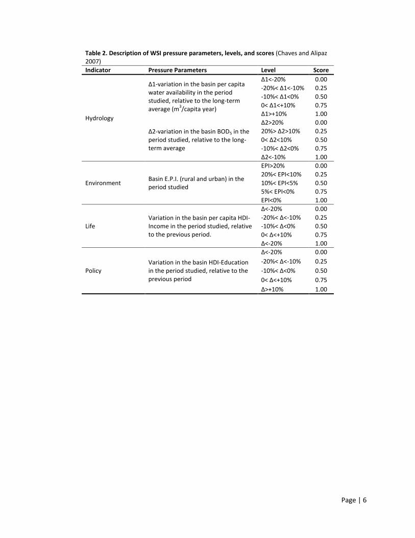
among stakeholders (Chaves and Alipaz 2007). WSI pressure parameters (Table 2) and state

parameters (Table 3), levels, and scores are clearly defined and tabulated allowing for users to

choose the best possible score for each parameter. However, the use of the model depends on

available information specific to watersheds, which may not be available in many regions.

Application of this on a global scale may not be feasible.

Figure 1 Global geography of incident threat to human water security (Vorosmarty, et al. 2010).

Page | 6

Table 2. Description of WSI pressure parameters, levels, and scores (Chaves and Alipaz 2007)

Indicator Pressure Parameters Level Score

Hydrology

Δ1-variation in the basin per capita water availability in the period studied, relative to the long-term average (m

3/capita year)

Δ1<-20% 0.00

-20%< Δ1<-10% 0.25

-10%< Δ1<0% 0.50

0< Δ1<+10% 0.75

Δ1>+10% 1.00

Δ2-variation in the basin BOD5 in the period studied, relative to the long-term average

Δ2>20% 0.00

20%> Δ2>10% 0.25

0< Δ2<10% 0.50

-10%< Δ2<0% 0.75

Δ2<-10% 1.00

Environment Basin E.P.I. (rural and urban) in the period studied

EPI>20% 0.00

20%< EPI<10% 0.25

10%< EPI<5% 0.50

5%< EPI<0% 0.75

EPI<0% 1.00

Life Variation in the basin per capita HDI-Income in the period studied, relative to the previous period.

Δ<-20% 0.00

-20%< Δ<-10% 0.25

-10%< Δ<0% 0.50

0< Δ<+10% 0.75

Δ<-20% 1.00

Policy Variation in the basin HDI-Education in the period studied, relative to the previous period

Δ<-20% 0.00

-20%< Δ<-10% 0.25

-10%< Δ<0% 0.50

0< Δ<+10% 0.75

Δ>+10% 1.00

Page | 7

Table 3. Description of WSI state parameters, levels, and scores (Chaves and Alipaz 2007)

Indicator State Parameters Level Score

Hydrology

Basin per capita water availability (m3/ capita

year) considering both surface and

groundwater sources

Wa<1,700 0.00

1,700< Wa<3,400 0.25

3,400< Wa<5,100 0.50

5,100< Wa<6,800 0.75

Wa>6,800 1.00

Basin averaged long term BOD5 (mg/l)

BOD>10 0.00

10< BOD<5 0.25

5< BOD<3 0.50

3< BOD<1 0.75

BOD<1 1.00

Environment Percent of basin area under natural vegetation

(Av)

Av<5 0.00

5< Av<10 0.25

10< Av<25 0.50

25< Av<40 0.75

Av>40 1.00

Life Basin HDI (weight by county population)

HDI<0.5 0.00

0.5< HDI<0.6 0.25

0.6< HDI<0.75 0.50

0.75< HDI<0.9 0.75

HDI>0.9 1.00

Policy Basin institutional capacity in IWRM (legal

and organizational)

Very poor 0.00

Poor 0.25

Medium 0.50

Good 0.75

Excellent 1.00

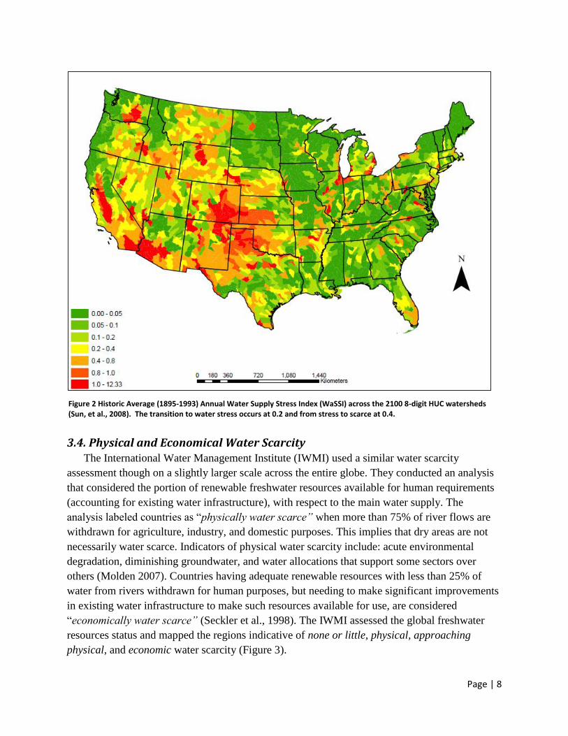
3.3. The Water Supply Stress Index McNulty et al., (2010) proposed a new hydrologic term to quantitatively assess the relative

magnitude of water supply and demand at the 8-digit USGS Hydrologic Unit Code (HUC) level.

This new term is the Water Supply Stress Index (WaSSI) and is similar to the WTA

methodologies (Eq. 4).

(4)

Water demand is WD, water supply is WS, and x represents either historic or future water supply

and/or demand from environmental and anthropogenic sectors. The WaSSI was calculated for

each 8-digit HUC watershed in the United States (Figure 2) and highlights water stressed areas

that are typically overlooked in assessments of larger scales. WaSSI is unique from other water

availability measurement tools in that factors in anthropogenic water demand. Therefore, it is

possible to have areas with high annual levels of precipitation to have a high WaSSI value.

Page | 8

3.4. Physical and Economical Water Scarcity The International Water Management Institute (IWMI) used a similar water scarcity

assessment though on a slightly larger scale across the entire globe. They conducted an analysis

that considered the portion of renewable freshwater resources available for human requirements

(accounting for existing water infrastructure), with respect to the main water supply. The

analysis labeled countries as “physically water scarce” when more than 75% of river flows are

withdrawn for agriculture, industry, and domestic purposes. This implies that dry areas are not

necessarily water scarce. Indicators of physical water scarcity include: acute environmental

degradation, diminishing groundwater, and water allocations that support some sectors over

others (Molden 2007). Countries having adequate renewable resources with less than 25% of

water from rivers withdrawn for human purposes, but needing to make significant improvements

in existing water infrastructure to make such resources available for use, are considered

“economically water scarce” (Seckler et al., 1998). The IWMI assessed the global freshwater

resources status and mapped the regions indicative of none or little, physical, approaching

physical, and economic water scarcity (Figure 3).

Figure 2 Historic Average (1895-1993) Annual Water Supply Stress Index (WaSSI) across the 2100 8-digit HUC watersheds (Sun, et al., 2008). The transition to water stress occurs at 0.2 and from stress to scarce at 0.4.

Page | 9

4. Indices Incorporating Environmental Water Requirements The Dublin Conference in 1991 concluded that “since water sustains all life, effective

management of water resources demands a holistic approach, linking social and economic

development with protection of natural ecosystems” (ICWE, 1992). Sullivan (2002) noted that

depleted freshwater resources are linked to ecosystem degradation, and therefore, any index of

water poverty should include the condition of ecosystems that maintain sustainable levels of

water availability. The proposed water poverty index incorporates ecosystem productivity,

community, human health, and economic welfare (Vorosmartyet al., 2005). However, this

approach is critically dependent on the development of standardized weights to be applied to

each of the variables previously mentioned. The problem therein lies with the basis of these

weights as well as the assumption that the weights hold true for all ecosystems, communities,

economies, and cultures.

4.1. Population Growth Impacts on Water Resource Availability Asheesh (2003) developed a scarcity index that measures the change in the water availability

of an area. Population growth rate, water availability, domestic, industrial and ecological water

usage, are all incorporated in the water scarcity index (Wsci). The magnitude of the water deficit

Figure 3 Areas of physical and economical water scarcity on a basin level in 2007 (IWMI 2008).

Page | 10

that must be returned into the system in order to sustain the balance between available water and

water demand is then evaluated (Eq. 5).

(

(

) ( )(

)

) (5)

Where annual freshwater availability α, annual per capita domestic demand ε, annual per capita

demand for green areas γ as a function of population growth, irrigation water demands δ,

population growth rate λ given by ln(1+r), population β, time t, annual evapotranspiration h,

environmental water requirements b, estimated freshwater losses k, and industrial water demand

p.

4.2. Assessing Water Resource Supplies Using the Water Stress Indicator A Water Stress Indicator (WSI) developed by Smakhtin, et al. (2005) recognizes

environmental water requirements as an important parameter of available freshwater. Mean

annual runoff (MAR) is used as a proxy for total water availability, and estimated environmental

water requirements (EWR) are expressed as a percentage of long-term mean annual river runoff

that should be reserved for environmental purposes (Eq. 7). Using global annual water

withdrawal data from the FAO and the IWMI for industrial, agricultural, and domestic sectors,

global water resources incorporating environmental water requirements were evaluated (Table

4). These results were compared to the previous assessment of a commonly used water stress

indicator (Eq. 6) that neglects EWRs (Figure 4). The authors applied this index in their global

water resources assessment analysis using the WaterGAP 2 tool. The comparison of the maps

illustrates that more basins show a higher magnitude of water stress when considering ecosystem

water requirements, thus providing a more accurate assessment of regional water resource

supplies.

(6)

(7)

Table 4. Categorization of environmental water scarcity (Smakhtin, et al., 2005)

WSI (proportion) Degrees of Environmental Water Scarcity of River Basins

WSI > 1 Overexploited (current water use is tapping into EWR)—environmentally water scarce

basins.

0.6 ≤ WSI < 1 Heavily exploited (0 to 40% of the utilizable water is still available in a basin before

EWR are in conflict with other uses)—environmentally water stressed basins.

0.3 ≤ WSI < 0.6 Moderately exploited (40% to 70% of the utilizable water is still available in a basin

before EWR are in conflict with other uses).

WSI < 0.3 Slightly exploited

Page | 11

5. LCA and Water Footprint

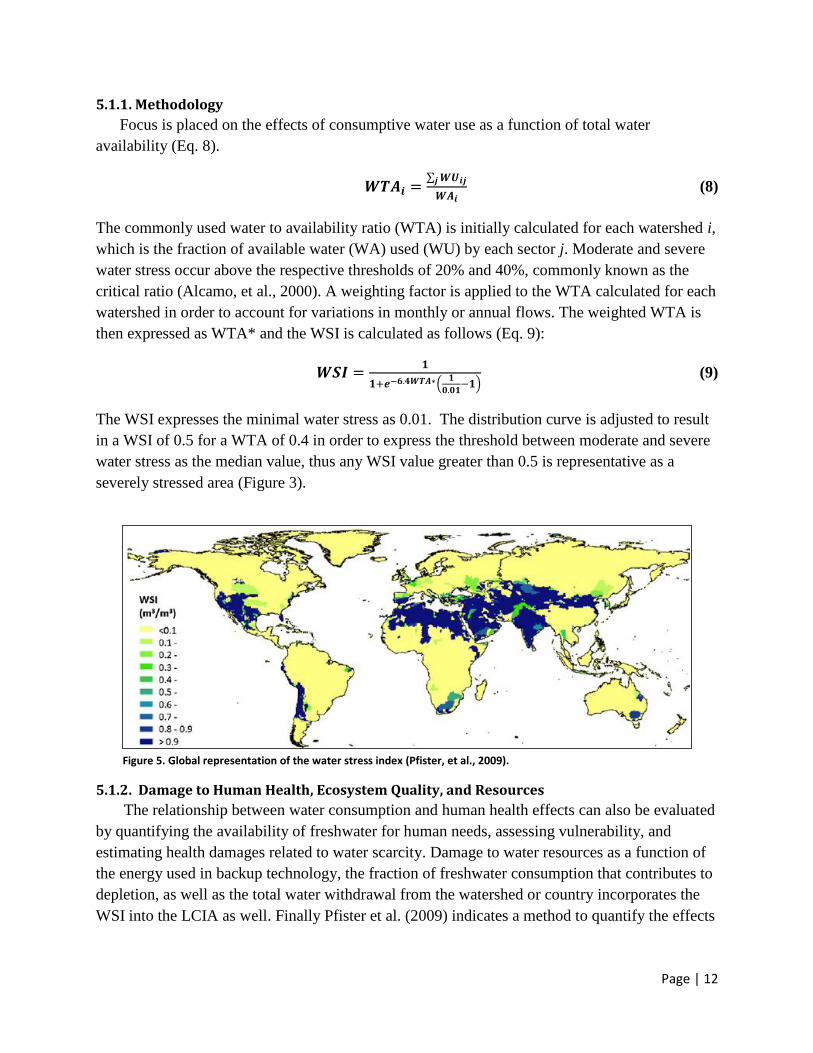
5.1. Life Cycle Assessment and WSI Pfister et al. (2009) utilized the Water Scarcity Index (WSI) as a general screening indicator

or characterization factor for water consumption used in Life Cycle Impact Assessment (LCIA)

as a means to measure potential environmental damages of water use for three areas: human

health, ecosystem quality, and resources. The damage assessments are performed according to

the framework of the Eco-Indicator-99 assessment methodology (Goedkoop and Spriensma

2001) .

Figure 4 (Top) A map of the “traditional” water stress indicator (water withdrawals as a proportion of the mean annual river runoff). (Bottom) A map of a water stress indicator which accounts for EWR. Areas shown in red are those where EWR presented in the top figure may not be satisfied under current water use. Most of the areas with variable flow regimes (and consequently the modest EWR of 20-30% of MAR) fall into the areas of environmental water scarcity. The circles include example river basins which can move into a higher category of human water scarcity, if EWR are to be satisfied. The risk of not meeting EWR will remain high in these basins, particularly as water withdrawals grow (Smakhtin, et al., 2005).

Page | 12

5.1.1. Methodology

Focus is placed on the effects of consumptive water use as a function of total water

availability (Eq. 8).

∑

(8)

The commonly used water to availability ratio (WTA) is initially calculated for each watershed i,

which is the fraction of available water (WA) used (WU) by each sector j. Moderate and severe

water stress occur above the respective thresholds of 20% and 40%, commonly known as the

critical ratio (Alcamo, et al., 2000). A weighting factor is applied to the WTA calculated for each

watershed in order to account for variations in monthly or annual flows. The weighted WTA is

then expressed as WTA* and the WSI is calculated as follows (Eq. 9):

(

)

(9)

The WSI expresses the minimal water stress as 0.01. The distribution curve is adjusted to result

in a WSI of 0.5 for a WTA of 0.4 in order to express the threshold between moderate and severe

water stress as the median value, thus any WSI value greater than 0.5 is representative as a

severely stressed area (Figure 3).

5.1.2. Damage to Human Health, Ecosystem Quality, and Resources

The relationship between water consumption and human health effects can also be evaluated

by quantifying the availability of freshwater for human needs, assessing vulnerability, and

estimating health damages related to water scarcity. Damage to water resources as a function of

the energy used in backup technology, the fraction of freshwater consumption that contributes to

depletion, as well as the total water withdrawal from the watershed or country incorporates the

WSI into the LCIA as well. Finally Pfister et al. (2009) indicates a method to quantify the effects

Figure 5. Global representation of the water stress index (Pfister, et al., 2009).

Page | 13

of freshwater consumption on terrestrial ecosystem quality. All of the above mentioned damage

assessments are performed according to the Eco-Indicator-99 methodology.

5.2. Water Footprinting Hoekstra (2003) introduced the water footprint concept as an indicator of freshwater use. The

indicator parameters include both direct water use by consumer and producers, as well as indirect

water use. The water footprint of a product is defined as “the volume of freshwater used to

produce the product, measured over the full supply chain.” Recently Hoekstra et al. (2009)

developed a method of calculating water scarcity by incorporating green, blue and grey water

footprints. Water scarcity is evaluated in terms of green water scarcity and blue water scarcity as

well as grey water production. The green water scarcity in a region is calculated as the ratio of

the green water footprint in the region and the green water availability. Likewise, the blue water

scarcity is the ratio or the blue water footprint to the blue water availability. The new concept of

„water pollution level‟ is an indicator of the magnitude of water flow pollution using grey water.

Polluted water is considered unusable water and is not included when calculating water resource

availability. Hoekstra et al. (2009) point out the common errors made in previously developed

indices:

1. Water withdrawals partly return to a catchment. Thus, using water withdrawal as the

primary indicator of water use is not a good method to evaluate the effect of the

withdrawal at the scale of the catchment as a whole. Instead, blue water consumption in

a region should be expressed in terms of a blue water footprint.

2. Water availability should not be solely defined by total runoff because it ignores the

fraction of the runoff required to maintain the environment. The environmental demand

should be subtracted from the total runoff.

3. Evaluating water scarcity as a function of annual usage and resource availability does

not account for variations during the year. It would be more accurate to consider

monthly values.

The overall assessment of water scarcity can be obtained by adding all of the water

footprints. The water scarcity can be evaluated at local, river basin, and global levels while

incorporating ecological, socio-economical, policy, and human impacts by using this water

footprinting method.

5.3. A Revised Approach to Water Footprinting Ridoutt et al. (2010) compare the carbon and water footprint concepts and suggest the

improvement of the water footprinting methodology in order to make it a more useful tool for

sustainable analysis. The major impacts of incorporating water consumption into product life

cycles were evaluated. It is suggested that the potential damage to freshwater ecosystem quality

through reduced environmental flows be the primary focus.

Page | 14

Carbon footprinting is acknowledged as an overall simplistic concept, as the emissions from

all major greenhouse gasses are additive and expressed as a single figure in the units of carbon

dioxide equivalents. Many water footprints are expressed as a single figure (Hoekstra et al.,

2009); however, they are not configured using a standardization process (Ridoutt et al., 2010).

Furthermore, many published water footprints are a raw collective of all forms of water

consumption: blue, green, and even dilution of water (Hoekstra et al., 2009). The authors argue

that different kinds of water consumption should not be simply added to produce a total water

footprint because the opportunity cost and the impacts associated with each form of freshwater

consumption differ.

Carbon footprints are also useful tools because they are comparable with the „global warming

potential midpoint indicator‟ used in life cycle assessment. In this way, carbon footprinting is a

modernized form of LCA. On the other hand, water footprints of different products are not

comparable since they vary in social and/or environmental impacts from life cycle water

consumption (Ridoutt et al., 2009).

Freshwater scarcity is a localized characteristic and the state of water availability for an area

cannot be assumed as the overall condition of a larger encompassing region. With carbon

footprinting, multiple greenhouse gases combine to form a resulting contribution to global

warming regardless of the location where they are produce. However, water footprinting

requires regional impact factors. Obviously, the impact of water consumed in a region of water

abundance is in no way comparable to water use where scarcity exists.

In order to be used as a useful influence towards sustainable consumption and production

like carbon footprinting, the water footprinting concept is in need of further extensive

development. An agreement must be made on the impact category or categories that are relevant

to freshwater withdrawals used in the water footprinting process. With this agreement, advances

in life cycle impact assessment will incorporate freshwater consumption and provide a standard

model as a useful sustainability measurement tool (Ridoutt et al., 2009). The appropriated

impacts of water consumption with respect to product life cycles are suggested below.

Social impacts of green water use

1. Occupation of the land limits the availability of the land and thereby access to green

water for other social purposes.

2. Land use influences the partitioning between green and blue water and thereby the

availability of blue water for other social purposes

3. Land use change has the potential to alter rates of runoff and thereby increase risks of

flooding.

Social Impacts of blue water use

1. Industrial users regularly compete for access to the local freshwater resources.

Page | 15

2. Use of non-renewable blue water from fossil groundwater resources limits the availability

of these resources for future generations.

Environmental impacts of green water use

1. Land transformation and occupation influence the partitioning between green and blue

water and thereby the availability of blue water for environmental flows.

2. Additional green water for food production can be accessed by conversion of natural

ecosystems into agricultural land. In this case, the impact is loss of natural ecosystems

and habitat.

Environmental impacts of blue water use

1. Water for irrigation and industrial use competes with water for the environment and can

lead to insufficient environmental flows with impacts on aquatic biodiversity as well as

riparian, floodplain and estuarine ecosystems.

2. Surface water used for irrigation directly reduces stream flows.

3. Irrigation may also raise the water table, which in turn can lead to salinity and water

logging.

4. Where groundwater systems support natural springs, depletion can cause these to dry up

resulting in damage to local ecosystems and loss of biodiversity.

Ridoutt et al. (2010) propose that the main concern relating to water consumption in agri-

food product life cycles is the potential to damage freshwater ecosystem health through reduced

environmental flows. The next action is to inventory the volume of blue water consumed in each

hydrologically-defined region (watershed or basin), followed by characterization factors applied

to reflect the local water stress; a similar approach to Pfister et al. (2009). This could potentially

derive standardized water footprint values that are comparable from one product to another.

6. Conclusion The methodology used for measuring water scarcity has evolved over the past twenty years.

The initial water scarcity threshold developed by Falkenmark in 1989 was an important

foundation on which water consumption demands were built. Recognizing that water

consumption varies among social sectors led Gleick and Falkenmark to further develop the water

scarcity index by incorporating specific water requirements for basic human needs. As

population increased, Asheesh (2003) suggested the link between water resource demand and

projected population growth as a way to measure gaps in water availability. Continued increase

in domestic water withdrawals and demands led to the recognition of the importance of water

necessary for ecological sustainability (Sullivan, 2002; Vorosmarty et al., 2005; Chaves &

Alipaz, 2007). The damages caused by water consumption were evaluated by Pfister et al. (2009)

followed by the proposition to measure water stress of an area based on ecological quality.

Another method used to measure water stress using water footprints was proposed by Hoekstra et

al. (2003) by calculating the respective blue, green, and grey water footprints of an area. This

Page | 16

serves as the best holistic approach when regarding all socio-economic, ecological, and industrial

factors; however, Ridoutt et al. (2009) suggest that the water footprinting method needs to be

improved in order to create a standardized model allowing for the comparison of footprints

between areas, products, etc. and proposed an alternative approach to water footprinting by

combining the water footprints with the Water Stress Index developed by Pfister et al. (2009).

Page | 17

References Alcamo, Joseph, Thomas Henrichs, and Thomas Rosch. World Water in 2025: Global modeling and

scenario analysis for the World Commission on Water for the 21st Century. Kassel World Water

Series Report No. 2, Center for Environmental Systems Research, Germany: University of Kassel,

2000, 1-49.

Asheesh, Mohamed. "Allocating the Gaps of Shared Water Resources (The Scarcity Index) Case Study

Palestine Israel." IGME, 2003: 797-805.

Chaves, Henrique M. L, and Suzana Alipaz. "An Integrated Indicator Based on Basin Hydrology,

Environment, Life, and Policy: The Watershed Sustainability Index." Water Resour Manage

(Springer) 21 (2007): 883-895.

Falkenmark. "The massive water scarcity threatening Africa-why isn't it being addressed." Ambio 18, no.

2 (1989): 112-118.

Falkenmark, M, and C Widstrand. Population and Water Resources: A Delicate Balance. Population

Bulletin, Population Reference Bureau, 1992.

Falkenmark, Malin. "Rapid Population Growth and Water Scarcity: The Predicament of Tomorrow's

Africa." Population and Development Review (Population Council) 16 (1990): 81-94.

FAO. AQUASTAT: Water Use. 2010. http://www.fao.org/nr/water/aquastat/water_use/index6.stm

(accessed June 2010).

Gleick, Peter H. "Basic Water Requirements for Human Activities: Meeting Basic Needs." Water

International (IWRA) 21 (1996): 83-92.

Gleick, Peter H. Water and Conflict: Fresh Water Resources and International Security. Oakland: Pacific

Institute, 1993, 79-112.

Gleick, Peter. "Human Population and Water: To the limits in the 21st Century." Human Population and

Water, Fisheries, and Coastal Areas. Washington, D.C.: American Association for the

Advancement of Science Symposium, 1995.

Goedkoop, M, and R Spriensma. "The Eco-Indicator 99: a Damage Oriented Method for Life Cycle Impact

Assessment: Methodology Report." 2001.

Hoekstra, A.Y. Virtual Water Trade: Proceedings of the Internatinal Expert Meeting on Virtual Water

Trade. Value of Water Research Report Series No. 12, Delft, The Netherlands: UNESCO-IHE,

2003.

Hoekstra, Arjen Y, Ashok K Chapagain, Maite M Aldaya, and Mesfin M Mekonnen. Water Footprint

Manual. Enschede: The Water Footprint Network, 2009.

Page | 18

International Conference on Water and the Environment. "The Dublin statement and record of the

Conference." WMO. Geneva, 1992.

IWMI. "Areas of physical and economic water scarcity." UNEP/GRID-Arendal Maps and Graphics Library,

2008.

Kalbermatten, J.M, D.S Julius, C.G Gunnerson, and D.D Mara. Appropriate Sanitation Alternatives: A

Planning and Design Manual. World Bank Studies in Water Supply and Sanitation 2, 1982.

McNulty, Steven, Ge Sun, Jennifer Moore Myers, Erika Cohen, and Peter Caldwell. "Robbing Peter to Pay

Paul: Tradeoffs Between Ecosystem Carbon Sequestration and Water Yield." Proceeding of the

Environmental Water Resources Institute Meeting. Madison, WI, 2010. 12.

Molden, David. A Comprehensive Assessment of Water Management in Agriculture. Internatinoal Water

Management Institute, Colombo, Sri Lanka: IWMI, 2007.

Nemani, R.R, et al. "Climate-driven increases in global terrestrial net primary production from 1982 to

1999." Science 300, no. 5625 (2003): 1560-1563.

Ohlsson, L. "Water Conflicts and Social Resource Scarcity." Phys. Chem. Earth 25, no. 3 (2000): 213-220.

Pfister, Stephan, Annette Koehler, and Stefanie Hellweg. "Assessing the Environmental Impacts of

Freshwater Consumption in LCA." Environmental Science & Technology (American Chemical

Society) 43 (2009): 4098-4104.

Raskin, P, P Gleick, P Kirshen, G Pontius, and K Strzepek. Waer Futures: Assessment of Long-range

Patterns and Prospects. Stockholm, Sweden: Stockholm Environment Institute, 1997.

Ridoutt, BG, SJ Eady, J Sellahewa, L Simons, and R Bektash. "Product Water Footprinting: How

Transferable Are The Concepts From Carbon Footprinting?" 2009.

Rijsberman, Frank R. "Water scarcity: Fact or Fiction?" Agricultural Water Management 80 (2006): 5-22.

Seckler, David, David Molden, and Randolph Barker. Water Scarcity in the Twenty-First Century. Water

Brief 1, International Water Management Institute, Colombo, Sri Lanka: IWMI, 1998.

Shiklomanov, I.A. "World fresh water resources." Water in Crisis: A Guide to the World's Fresh Water

Resources, 1993.

Smakhtin, V, C Revanga, and P Doll. "Taking into Account Environmental Water Requirements in Global-

scale Water Resources Assessments." IWMI The Global Podium. 2005.

http://podium.iwmi.org/podium/Doc_Summary.asp (accessed June 2010).

Sullivan, Caroline. "Calculating a Water Poverty Index." World Development (Elsevier Science Ltd) 30, no.

7 (2002): 1195-1210.

Page | 19

Sun, G, S McNulty, J.A Moore Myers, and E.C Cohen. "Impacts of Climate Change, Population Growth,

Land Use Change, and Groundwater Availability on Water Supply and Demand Across the

Conterminous U.S." Watershed Update (AWRA Hydrology & Watershed Management Technical

Committee) 6, no. 2 (May-July 2008): 28.

Vorosmarty, C.J, et al. "Global Threats to Human Water Security and River Biodiversity." Nature

(Macmillan Publishers Limited) 467 (September 2010): 555-561.

Vorosmarty, Charles J, Ellen M Douglas, Pamela A Green, and Carmen Revenga. "Geospatial Indicators of

Emerging Water Stress: An Application to Africa." Ambio (Royal Sweedish Academy of Sciences)

34, no. 3 (May 2005): 230-236.

Yang, H, and J.B Zehnder. "Water Scarcity and Food Import: A Case Study for Southern Mediterranean

Countries." World Development 30, no. 8 (2002): 1413-1430.

Yang, Hong, Peter Reichert, Karim C Abbaspour, and Alexander J.B Zehnder. "A water resources

threshold and its implications for food security." Environmental Science & Technology (American

Chemical Society) 37 (2003): 3048-3054.