(high-order) finite elements for the shallow-water ...dubos/talks/2014kritsikispdes.pdf ·...
TRANSCRIPT

(High-order) �nite elements for the shallow-waterequations on the cubed sphere
E.Kritsikis, T. Dubos
University of Paris 13 & LMD � Ecole polytechnique
PDEs on the Sphere 2014

Plan
1 Formulation
2 Fixing the spectral gap
3 Sphering the cube
4 Results
2/18

The problem
Shallow water
∂th +∇ · U = 0 , U = hu
∂tu + qU⊥ +∇B = 0 , B = hg + u2/2
Questions
ensure the conservation requirements (mass, energy, momentum, PV)
get good dispersion properties
do it on the sphere
Formulation 3/18

The Hamiltonian structureH(u, h) = 1
2
∫h(gh + u2)
The Poisson bracket
dF
dt= {F ,H} =
∫q ·(∂F
∂u× ∂H
∂u
)+∂H
∂hdiv
∂F
∂u− ∂F
∂hdiv
∂H
∂u
track evolution of any F (h, u)recover eqs of motion if U := ∂H/∂u, B := ∂H/∂hantisymmetry → energy conservation
Procedure
de�ne (U,B) on U ′ ×H′ i.e. as functional derivatives of H
(δu,U) + (δh,B) = δH
de�ne antisymmetric bilinear form J on U ′ ×H′ s.t.
∂t(U, u) + ∂t(B, h) = J((
UˆBˆ
),(UB
))= (q, U × U) + (B, div U)− (B, divU)
Formulation 4/18

Spaces (Cotter & Shipton '13)
u,U ∈ Uh,B ∈ Hlose regularity going left to right
Z∇⊥ // Urotoo
div // H∇oo
Formulations
Solve ∀u ∈ U , (U, u) = (hu, u)
Compute ∂th = − divU
Compute (for discr.) ∀h ∈ H, the (B, h) = (u2/2+ hg , h)
Solve ∀q ∈ Z, (qh, q) = (∇⊥q, u)Solve ∀U ∈ U , (U, ∂tu) + (U, qU⊥)− (div U,B) = 0
Note : we have (q, ∂t(hq)) = (∇⊥q, ∂tu) = (∇⊥q, qU⊥) = (q, curl(qU⊥)),weak form of the PV transport ∂t(hq) + div(qU) = 0.
Formulation 5/18

FE spaces
Triangle mesh + RT
P1∇⊥ // RT0
div // Pd0
2N div. vs N rot. DOFs ⇒ numerical modes(Gaÿmann '12)
Quad mesh + ⊗
A∂x // B
Pn Pn−1 (?)
A⊗A ∇⊥ // A⊗ B~ι+ B ⊗A~j div // B ⊗ B
Fixing the spectral gap 6/18

Linear analysis for P2 − Pd1
Regular periodic 1D, (h, u, v) ∼ exp i(kx − ωt)ω = 0 : transport of PV ⇒ geostrophic balanceω2 = f 2 + gH k2 : 2 DOFs per element breaks translational invariance ⇒spectral gap
0 10 20 30 4010
15
20
25
30
35
40
N
ωc=1 f=10
DG1
continuous
(Melvin '13)
Fixing the spectral gap 7/18

Fixing the spectral gap : the �FDn − FVn−1� pair
let B be the image of a reconstruction operator (hk) 7→ h s.t.∫ xk+1
xk
h(x) dx = hk
e.g. a nth order FV reconstruction with h ∈ Pdn−1
a basis is bk(x) with∫ xj+1
xj
bk(x) dx = δjk −→ h =∑k
bk(x)
∫ xk+1
xk
h(x) dx
let A be the span of the
ak(x) =
∫ x
−∞(bk+1(x
′)− bk(x′)) dx ′
h 7→∑
k h(xk)ak(x) is a nth order
interpolation and A ∂x→ B−2 0 2 4
−0.5
0
0.5
1
1.5
a(x)
b(x)
Fixing the spectral gap 8/18

Fixing the spectral gap : the �FD2 − FV1� pair
0 10 20 30 4010
15
20
25
30
35
40
N
ω
c=1 f=10
DG1
continuous
Extends to arbitrarily-high order (but stencil increases)
Fixing the spectral gap 9/18

Fixing the spectral gap : the �FD2 − FV1� pair
0 10 20 30 4010
15
20
25
30
35
40
N
ω
c=1 f=10
FV1
continuous
Extends to arbitrarily-high order (but stencil increases)
Fixing the spectral gap 9/18

Wave velocities
Fixing the spectral gap 10/18
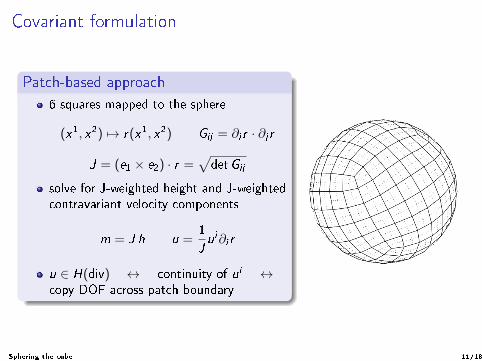
Covariant formulation
Patch-based approach
6 squares mapped to the sphere
(x1, x2) 7→ r(x1, x2) Gij = ∂i r · ∂j r
J = (e1 × e2) · r =√detGij
solve for J-weighted height and J-weightedcontravariant velocity components
m = J h u =1
Jui∂i r
u ∈ H(div) ↔ continuity of ui ↔copy DOF across patch boundary
Sphering the cube 11/18

Covariant formulation
Hamiltonian
H(uj ,m) =1
2
∫m
(gm
J+
Gij
J2ujui
)B =
δHδm
=gm
J+
Gij
2J2ujui
U i =δHδui
=m
Jui = hui
Poisson bracket
δF =
∫Gij
J
δFδui
δuj +δFδm
δm
{F ,H} = J((
δF/δui
δF/δm
),(δH/δui
δH/δm
))J((
Uˆi
Bˆ
),(Uˆi
B
))= εijqU
iU j +
∫B∂i U
i − B∂iUi
Sphering the cube 12/18

The weak and the strong
Zεij∂j // U i
∂i // M , Z = A⊗A, U1 = A⊗ B, U2 = B ⊗A, M = B ⊗ B
(U j ,
Gij
JU i
)=
(U j ,
Gij
J2mui
), U i ,U i ∈ U i
(m,B) =
(m
(g
Jm +
1
2
Gij
J2ujui
)), m,B ∈M(
ψm, q)=
(ψJf − εik Gij
Juj∂k ψ
), ψ, q ∈ Z(
U i ,Gij
J∂tu
j
)+(U i , εijU
jq)−(B∂i u
i)= 0, U i , ui ∈ U i
∂tm + ∂iUi = 0
Strong cont. eq. → can be coupled to FV transport schemes
Sphering the cube 13/18

FD3/FV2 : basis functions
Results 14/18

FD3/FV2 : order of individual operators
101
102
10−10
10−8
10−6
10−4
10−2
0−form
L
∞
error
4−th order
101
102
10−6
10−5
10−4
10−3
10−2
1−form
L
∞
error
3rd order
101
102
10−10
10−8
10−6
10−4
10−2
curl
L
∞
error
4th order
101
102
10−5
10−4
10−3
10−2
10−1
Laplacian
L
∞
error
2nd order
Results 15/18

Results : rotating shallow-water
test cases from Williamson et al. (1991)
3rd-order convergence for solid-body rotation, other tests closer to 2nd-order
Results 16/18

Results : Galewsky test-case
Results 17/18

Summary
Discretize Hamiltonian, Poisson bracket
Mimetic properties result from exact suites
Use quadrangles to balance DOFs and avoid numerical modes
Standard higher-order spaces su�er from spectral gap
Use 1 DOF per element to restore discrete translational invariance
New 1D spaces based on interpolation-reconstruction operators
Promising results on cubed sphere
Ongoing work : stabilization, e�ciency
Results 18/18