AFRL-IF-RS-TR-2006-49

Final Technical Report

February 2006

EYE DETECTION AND TRACKING FOR INTELLIGENT HUMAN COMPUTER INTERACTION State University of New York at Binghamton

APPROVED FOR PUBLIC RELEASE; DISTRIBUTION UNLIMITED.

AIR FORCE RESEARCH LABORATORY INFORMATION DIRECTORATE

ROME RESEARCH SITE ROME, NEW YORK

STINFO FINAL REPORT This report has been reviewed by the Air Force Research Laboratory, Information Directorate, Public Affairs Office (IFOIPA) and is releasable to the National Technical Information Service (NTIS). At NTIS it will be releasable to the general public, including foreign nations. AFRL-IF-RS-TR-2006-49 has been reviewed and is approved for publication APPROVED: /s/

JASON A. MOORE Project Engineer

FOR THE DIRECTOR: /s/

JAMES W. CUSACK Chief, Information Systems Division Information Directorate

REPORT DOCUMENTATION PAGE Form Approved

OMB No. 074-0188 Public reporting burden for this collection of information is estimated to average 1 hour per response, including the time for reviewing instructions, searching existing data sources, gathering and maintaining the data needed, and completing and reviewing this collection of information. Send comments regarding this burden estimate or any other aspect of this collection of information, including suggestions for reducing this burden to Washington Headquarters Services, Directorate for Information Operations and Reports, 1215 Jefferson Davis Highway, Suite 1204, Arlington, VA 22202-4302, and to the Office of Management and Budget, Paperwork Reduction Project (0704-0188), Washington, DC 20503 1. AGENCY USE ONLY (Leave blank)

2. REPORT DATEFEBRUARY 2006

3. REPORT TYPE AND DATES COVERED Final May 2005 – Sep 2005

4. TITLE AND SUBTITLE EYE DETECTION AND TRACKING FOR INTELLIGENT HUMAN COMPUTER INTERACTION

6. AUTHOR(S) Lijun Yin

5. FUNDING NUMBERS C - FA8750-05-1-0182 PE - 62702F PR - 558B TA - II WU - RS

7. PERFORMING ORGANIZATION NAME(S) AND ADDRESS(ES) State University of New York at Binghamton Department of Computer Science Binghamton New York 13902

8. PERFORMING ORGANIZATION REPORT NUMBER

N/A

9. SPONSORING / MONITORING AGENCY NAME(S) AND ADDRESS(ES) Air Force Research Laboratory/IFSB 525 Brooks Road Rome New York 13441-4505

10. SPONSORING / MONITORING AGENCY REPORT NUMBER

AFRL-IF-RS-TR-2006-49

11. SUPPLEMENTARY NOTES AFRL Project Engineer: Jason A. Moore/IFSB/(315) 330-1588/ Jason.Moore @rl.af.mil

12a. DISTRIBUTION / AVAILABILITY STATEMENT APPROVED FOR PUBLIC RELEASE; DISTRIBUTION UNLIMITED.

12b. DISTRIBUTION CODE

13. ABSTRACT (Maximum 200 Words) Knowing the user’s eye location has significant potential to enhance current human computer interfaces, given that the eye movement can be used as an indicator for user’s attention. The goal of this research is to develop a new and robust approach of eye detection and tracking, which leads to a significant application for the intelligent computer interface design in the visualization and military training system. The ultimate goal of this research is to develop an intelligent system toward the next generation of human computer interaction. In this project, Dr. Lijun Yin has developed a new algorithm for detecting and tracking eyes under an unconstrained environment using a single ordinary camera or webcam. The new algorithm is advantageous in that it works in a non-intrusive way based on a so-called Topographic Context approach.

15. NUMBER OF PAGES28

14. SUBJECT TERMS Eye Tracking, Eye Detection, HCI, Computer Vision

16. PRICE CODE

17. SECURITY CLASSIFICATION OF REPORT

UNCLASSIFIED

18. SECURITY CLASSIFICATION OF THIS PAGE

UNCLASSIFIED

19. SECURITY CLASSIFICATION OF ABSTRACT

UNCLASSIFIED

20. LIMITATION OF ABSTRACT

ULNSN 7540-01-280-5500 Standard Form 298 (Rev. 2-89)

Prescribed by ANSI Std. Z39-18 298-102

i

Table of Contents 1. Introduction.................................................................................................................. 1

2. Topographic classification............................................................................................ 2

3. Learning GMM Based Classifier................................................................................. 5

4. Mutual Information Based Eye Tracking................................................................. 10

5. Experiments................................................................................................................. 14

6. Conclusions and Discussions ...................................................................................... 19

7. Acknowledgments ....................................................................................................... 20

8. References .................................................................................................................... 20

ii

List of Figures

Figure 1: Face image and the 3D terrain surface of the eye region. The surface level is inversed so that the peak denotes the pit in real surface. (a) original face image; (b) terrain surface of the eye region of the original image; (c) face image after Gaussian filter smoothing(filter size 15 × 15, σ =3.0); (d) terrain surface of the eye region of the smoothed image. 3 Figure 2: The topographic labels: The center pixel in each example carries the indicated label. (a) peak; (b) pit; (c) ridge; (d) ravine; (e) ridge saddle; (f) ravine saddle; (g) convex hill; (h) concave hill; (i) convex saddle hill; (j) concave saddle hill; (k) slope hill; and (l) flat. ...................................................................................................................................... 4 Figure 3: (a) The topographic classification of the pixels in the face region. (b) Only the pit-labeled pixels are displayed........................................................................................... 5 Figure 4: (a) The sample used as a positive training set, whose corresponding terrain patches are shown in (c); (b) The non-eye samples used as a negative training set, whose corresponding terrain patches are shown in (d) .................................................................. 6 Figure 5: Examples of eye detection from videos .............................................................. 9 Figure 6: Examples of eye detection from images.............................................................. 9 Figure 7: Frame i (a) and frame j (b) show the centers of pupils, denoted by (α, β) and (α’, β’), respectively.......................................................................................................... 10 Figure 8: Frame i (a) and frame j (b) show the terrain surfaces of the left eye patch in frame i and frame j. ........................................................................................................... 11 Figure 9: (a-b) The terrain maps of the frames i and j, where rectangles denotes the eye regions; (c) MI calculated on the jth frame as a function of the patch position. (d) The statistical dependency measured by the empirical mutual information of the jth frame. The white spot corresponds to the peak position of (c). ................................................... 12 Figure 10: Example of the eye detection and tracking program interface (The images are selected from the MMI database [30]).............................................................................. 14 Figure 11: Examples of eye detection on the JAFFE database [21]. ................................ 16

iii

Figure 12: Sample frames of detected and tracked eyes from a video sequence captured by a static web-cam. From top-left to bottom-right: frame 1, 20, 40, 60, 80, 100, 120, 140, 160, 180, 200, and 220.............................................................................................. 17 Figure 13: Sample frames of detected and tracked eyes from a video sequence captured by an active web-cam. From top-left to bottom-right: frame 1, 20, 40, 60, 80, and 100.. 18

1

1. Introduction Facial feature detection is critical for many face-related applications, such as face recognition, face expression understanding, human computer interaction, etc. The facial features refer to the prominent features such as face-eyebrows, eyes, nose, mouth, and chin. Among the facial features, eyes play a significant role for delivering interactive signals and revealing the intention or instructions of a user. Eye features are relative steady as well as informative. There is intensive research for finding faces and detecting eyes. In the past, most of approaches required to restrict the regions of interesting for locating facial features. Then geometrical information or texture information could be used to detect eyes. Especially, the deformable template based methods have good development in the past years. Research based on this kind of methods has been reported in [1, 2, 3, 4, 5, 25, 26, 27, 28]. These approaches for eye detection are computationally intensive the proper location of face region in advance. There are also some other methods for eye location without finding faces [7, 23, 24, 29]. A fractal dimensions based method can accurately locate eye pairs in complex images [6]. Z Zhou etc. applied projection function for eye detection [8]. Furthermore, some researchers have developed facial feature detection and tracking algorithms using the infrared lighting camera [9]. Because the iris of human eye has large reflection to infrared light, the infrared (IR) illumination based technique is widely employed for locating eyes [15, 16]. This approach is relatively effective and robust. However, it requires the special hardware with IR lighting cameras. The result of detection and tracking still depends on the various eye appearances (e.g., orientation, size and eye blinking, etc.) In order to improve the performance of eye tracking, Kalman filter [16] or Mean Shift techniques [17, 18, 19] can be applied as the alternative remedies for real time implementation with sufficient accuracy. As we know, because of the specific reflection characteristic of pupil, the centers of eyeballs are always fuscous. However, the white of eyeball exhibits light-colored. If the gray image is looked as a 3D surface with the height of each location denoted by the intensity of the corresponding pixel, the eye region shows certain terrain pattern. The center consists of pits, surrounded by hillside. This gives us a hint that the eye can be detected using its terrain features [10, 11]. In this project, we propose a novel method for eye detection:

• First, we derive the terrain maps from the original gray level image by applying a new method from topographic primal sketch theory.

• Second, we denote the pit points in the terrain map as the candidates for eye pair

selection.

2

• Third, a GMM (Gaussian Mixture Model) based possibility model is learned as a classifier to determine the eyes pair from the candidate points.

After determining the initial eye location, we can further proceed to track eyes through dynamically matching their surface patches between two adjacent frames. A mutual information (MI) based fitting function is constructed to estimate the similarity between two patches. Although the eye location can be tracked by optimizing the fitting function, it is computationally expensive if we exhaust all the possible matching in the search area. Alternatively, here we apply an efficient strategy to find the optimal feature match. We take advantage of the pit terrain features to compute the mutual information selectively in the terrain map domain. Using such a strategy brings twofold benefits:

• Firstly, the probability distribution function (p.d.f.) is much easier and more precise to be estimated in the terrain map domain than in the intensity domain because the terrain map has only twelve types of topographic features while intensity domain has 256 levels.

• Secondly, the optimal match can be usually found in the location of pit feature

pixels. This implies that for most of cases, we do not need to traverse all the pixels in the search area. Experiments on eye tracking show that the optimal match can be achieved for more than 98% of frames by searching only several pit pixels in real video sequences.

The rest of the report is organized as follows. In Section 2, the background of topographic classification of pixels for gray scale image is introduced. Section 3 provides the detailed feature extraction and classification model. Section 4 describes the eye-tracking algorithm, followed by the experiments in Section 5. The final discussion and conclusion will be given in Section 6. 2. Topographic classification In topographic primal sketch theory, a gray level image is treated as 3D terrain surface. The intensity I(x,y) is represented by the height of the terrain at pixel (x,y). Figure 1 shows an example of a face image and its terrain surface in the eye region.

3

(c) (d)

(a) (b)

Figure 1: Face image and the 3D terrain surface of the eye region. The surface level is inversed so that the peak denotes the pit in real surface. (a) original face image; (b) terrain surface of the eye region of the original image; (c) face image after Gaussian filter smoothing(filter size 15 × 15, σ =3.0); (d) terrain surface of the eye region of the smoothed image. As we know, the intensity variation on a two-dimensional face image is caused by the face surface orientation and its reflectance. The resulted texture appearance provides an important visual cue in order to classify a variety of facial regions and their features [14, 20]. If viewed as a 3D terrain surface, the face image shows some 'waves' in the face region because the facial surface has certain reflectance characteristics. For eyeball, it generally composed of two parts: the black part and the white part. The reflectance characteristics of eyeball exhibits in the 3D surface. The center consists of some pit features, surrounded by hillside features. Mathematically, we can give a strict definition for pits on a terrain surface. Assume that the continuous surface is represented by the equation z=f(x,y). Thus, the gradient magnitude ||),(|| yxf∇ can be computed as:

2),(2),( ][][||),(|| yyxf

xyxfyxf ∂

∂∂

∂ +=∇ (1)

Then, the Hessian matrix H is given as:

4

⎥⎥

⎦

⎤

⎢⎢

⎣

⎡=

∂

∂∂∂

∂∂∂

∂

∂

∂

2

22

2

2

2

),(),(

),(),(

),(y

yxfyx

yxfyx

yxfx

yxf

yxH (2)

After applying the eigenvalue decomposition to the Hessian matrix, we can get:

TT uudiaguuUDUH ][)(][ 212,121 ⋅⋅== λλ (3) Where 1λ and 2λ are the eigen-values and 1u and 2u are the orthogonal eigen-vectors. A pit feature appears where a local minim gradient is found, which means that the gradient is zero and the second directional derivative is positive in all directions:

0||),(|| =∇ yxf , 01 >λ and 02 >λ . Similarly, there are also other terrain types: peak, ridge, saddle, hill, flat, ravine, or pit [10]. Hill-labeled pixels can be further specified as one of the labels: convex hill, concave hill, saddle hill or slope hill, and saddle hills can be further distinguished as concave saddle hill or convex saddle hill, saddle as ridge saddle or ravine saddle. Figure 2 shows the twelve kinds of terrain labels. By using some smoothed differentiation filters, such as the filter based on discrete Chebyshev polynomials, to fit onto the discrete surface, the topographic labeling techniques can be easily to extend to discrete case [12]. The detailed topographic labeling rules for gray scale images can be found in [13].

Figure 2: The topographic labels: The center pixel in each example carries the indicated label. (a) peak; (b) pit; (c) ridge; (d) ravine; (e) ridge saddle; (f) ravine saddle; (g) convex hill; (h) concave hill; (i) convex saddle hill; (j) concave saddle hill; (k) slope hill; and (l) flat. The smoothing preprocessing on the gray scale image before calculating the derivatives is necessary for reducing the noise influence. In order to achieve the balance between eliminating noise and maintaining enough image details, it is vital to choose proper parameters of the smoothing filter. An example of a face image and its 3D surface of the

5

eye region after Gaussian smoothing processing are shown in Figure 1. In the example, a Gaussian filter with the size of 15 ×15, the standard deviation σ=3.

(a) (b)

Figure 3: (a) The topographic classification of the pixels in the face region. (b) Only the pit-labeled pixels are displayed. By applying topographic classification technique, the pixels in the original gray scale image are labeled by one of the twelve terrain classes based on its topographic feature. An example of the result of topographic classification is shown in Figure 3. The majority of face region is classified as hill labels. Although the pits-labeled pixels are sparsely distributed, it always appears in the eyeball regions. Based on the above analysis, we make a conclusion that the pits always occurs in the eye region if the image is smoothed by a proper filter without losing too much details. Accordingly, it is conceivable that the pit-labeled pixels are set as the candidates for eye detection. In general, we first merge some pits features which are closely located each other. This processing will dramatically decrease the number of candidates and reduce the computation for the subsequent classification. 3. Learning GMM Based Classifier In order to classify the candidate pit-labeled pixels, we take into account the terrain information around the pixels. Assume that the two points a and b are the centers of two eyeballs and the distance of the two eyes is calculated as d. Two rectangular eye patches with a size of 0.6d × 0.3d, centered at a and b are cut out. The topographic information of the two rectangles is applied for evaluating the possibility of the two points to be a pair of eyes. Theoretically, we must take all the pairs of pit-labeled candidates into account. However, because some pairs of candidates have unreasonable distances, those beyond the reasonable range of eye-pair distance can be ignored. The terrain feature of a reference pixel is discretized to the range of 1,2...M, which is corresponding to the

6

number of types of terrain labels. Thus, after vectorization, the terrain feature can be represented as

},...,...,,{ 21 Ni ttttt = (4)

Where Mti <<1 the terrain label of the pixel and N is is the number of pixels. The terrain feature can be visualized by gray image. Figure 4 shows some examples from our training data set.

(c) (d)

(a) (b)

Figure 4: (a) The sample used as a positive training set, whose corresponding terrain patches are shown in (c); (b) The non-eye samples used as a negative training set, whose corresponding terrain patches are shown in (d) A training set with 293 face images are constructed for the learning of classifier. First of all, based on the topographic classification, each pixels of the image are labeled by certain terrain labels. Then, all the pit-labeled pixels are marked as the candidates for training. Third, random pairs of candidates are selected as the training samples, which roughly consists of two groups: eye pairs and non-eye pairs. Figure 4 shows some examples of these two classes of samples. Because typically human eyes are

7

approximately symmetrical, there are a little difference in the terrain surface between left eye and right eye. During the learning, we treat left eye and right eye separately. Based on the Gaussian Mixture Model, all the samples, eye candidates and non-eye candidates are supposed to distribute in a high-dimensionality space obeying certain Gaussian distribution. Here we employ a Gaussian Mixture Model (GMM) to describe the property of the terrain feature vector. If we treat each terrain feature vector of pit pixels as a sample, GMM presumes all the samples distribute in a high-dimensional space complying with several Gaussian distributions. Among all the samples for both eye candidates and non-eye candidates, we can further categorize them into three sub-spaces, i.e., a left eye space, a right eye space and an non-eye space. Each of them is described by a Gaussian distribution. Let us define a subspace ξl for the left eye, ξr for the right eye and ψ for the non-eye candidates, with the probability distribution being

),( lll ΕΡ µ , ),( rrl ΕΡ µ , ),( uuu ΕΡ µ All these three subspaces constitute a sample space Ο , whose parameterized form is defined as:

},,;,,;,,{ uuurrrlll pppO ΕΕΕ= µµµ (5)

Where },,{ url ppp are the prior probabilities, },{ Εµ denote the mean and covariance matrix of the Gaussian distributions. Given a pair of candidates, a and b, with the terrain feature vectors being },{ ba tt , the posterior probability of the candidate pair belonging to the eye space

},{ rl ξξξ = (6)

is calculated as follow:

)|()|{)|()|{),|( arblbralba tptptptpttp ξξξξξ ⋅+⋅= (7) It can be represented as the following format:

)|{)|{

)|{)|{

)|{)|{

)|{)|{),|( Otp

ptpOtp

ptpOtp

ptpOtp

ptpba b

llb

a

rra

b

rrb

a

llattp ⋅⋅⋅⋅ ⋅+⋅= ξξξξξ (8) where the probability )|{),|{ OtpOtp ba are calculated as:

uarrallaa ptpptpptpOtp ⋅Ψ+⋅+⋅= )|()|()|()|( ξξ (9)

8

ubrrbllbb ptpptpptpOtp ⋅Ψ+⋅+⋅= )|()|()|()|( ξξ (10)

With the estimated parametric model, the real eye-pair can be extracted according to the maximum value of probability ),|( ba ttp ξ

))()(21exp(

)2(

1),|()|( 1eyeeye

Teye

eyedeyeeyepEp µµ

πµ −∑−−

∑=∑= − tttt (11)

We use a training set to learn the parameters of the probabilistic model. Among all the candidate pixels (pit-labeled pixels), we randomly select a pair of candidates, and generate a terrain patch for each candidate. After obtaining all the terrain patch vectors, we divide them into three sets, i.e., two positive sets including a group of left eyes and right eyes samples, respectively, and a negative set including a non-eye group. From the training set, the parameters in formulas 5 can be estimated. By using such a probability model, we are able to extract the eye-pair with a maximum probability value calculated by Equation 8. Note that during the classification of all candidate pixels, searching all possible pairs of candidates is a time-consuming process. In order to reduce the search space, we discard the pairs of candidates which have unreasonable distances between them (e.g., the distance of a pair of candidates is beyond the range of a normal eye-pair distance with respect to the given image size, or the orientation of the eye-pair is near the vertical direction.) As such, only a small number of pairs of candidates need be examined, and thus the computation load can be greatly reduced. Figure 5 shows four examples from the several frames of a videos, where the eyes of four subjects are detected correctly from a few of candidate pixels. The topographic eye location approach has certain robustness to unconstrained background. Note that through iteratively extracting the eye pairs and verifying the inter-pair appearance features, the eye location approach can be extended to solve multiple-face cases. Figure 6. shows the several samples for the eye detection.

9

Figure 5: Examples of eye detection from videos

Figure 6: Examples of eye detection from images

10

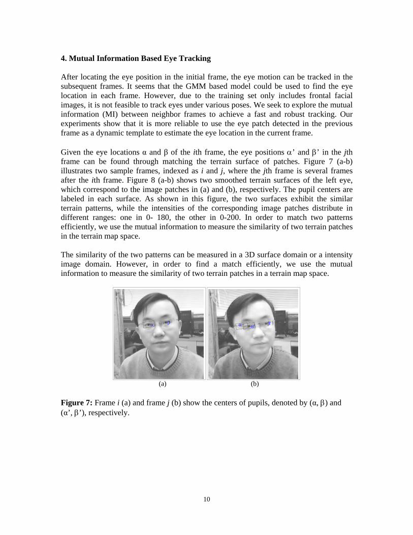
4. Mutual Information Based Eye Tracking After locating the eye position in the initial frame, the eye motion can be tracked in the subsequent frames. It seems that the GMM based model could be used to find the eye location in each frame. However, due to the training set only includes frontal facial images, it is not feasible to track eyes under various poses. We seek to explore the mutual information (MI) between neighbor frames to achieve a fast and robust tracking. Our experiments show that it is more reliable to use the eye patch detected in the previous frame as a dynamic template to estimate the eye location in the current frame. Given the eye locations α and β of the ith frame, the eye positions α’ and β’ in the jth frame can be found through matching the terrain surface of patches. Figure 7 (a-b) illustrates two sample frames, indexed as i and j, where the jth frame is several frames after the ith frame. Figure 8 (a-b) shows two smoothed terrain surfaces of the left eye, which correspond to the image patches in (a) and (b), respectively. The pupil centers are labeled in each surface. As shown in this figure, the two surfaces exhibit the similar terrain patterns, while the intensities of the corresponding image patches distribute in different ranges: one in 0- 180, the other in 0-200. In order to match two patterns efficiently, we use the mutual information to measure the similarity of two terrain patches in the terrain map space. The similarity of the two patterns can be measured in a 3D surface domain or a intensity image domain. However, in order to find a match efficiently, we use the mutual information to measure the similarity of two terrain patches in a terrain map space.

βα α β’α’

(a) (b) Figure 7: Frame i (a) and frame j (b) show the centers of pupils, denoted by (α, β) and (α’, β’), respectively.

11

(b)(a)0

1020

3040

50

0

10

20

30

40

500

50

100

150

200

α

010

2030

4050

0

10

20

30

40

500

20

40

60

80

100

120

140

160

180

α’

Figure 8: Frame i (a) and frame j (b) show the terrain surfaces of the left eye patch in frame i and frame j. Assume that two patches are centered at α and α’ and the corresponding terrain feature vectors are tα and tα’, which are represented by the random variables as X and Y, the mutual information between the two variables is calculated as:

∑∑=X Y aYaX

aaXYaaXY tPtP

ttPttPYXg

)()(),(

log),(),('

'

' (12)

In order to calculate the mutual information, we must estimate the marginal and joint p.d.f. of the random variables X and Y (where 1 < X, Y < 12). Because there are only 12 kinds of terrain labels rather than 256 levels in the intensity domain, it is fairly easy and fast to estimate the discrete p.d.f. PX, PY and PXY, which correspond to the normalized 1D and 2D histograms of the terrain map. As described in Section 2, the appearance based terrain features can be represented by a terrain map. Figure 9(a-b) illustrates the terrain maps of two patches corresponding to the two surfaces in Figure 9(c-d). Both regions are centered at the eye location α of the ith frame. The terrain patch is marked out by a rectangle along the direction of the detected eye-pair in the ith frame. Let pi= α denote the determined eye location in the ith frame and the variable p∈ P represent the current searching position in the (i+1)th frame, where P defines a search area. Then the mutual information can be defined as a function of the variable p, as shown in the following formula:

),()(),( yx ppgpgYXg == (13) Where ),( yx ppp = is a 2D coordinate of the patch center in the i+1th frame. The function g(p) does not have the explicit form, but it can be computed with the sampled p. Figure 9(c) plots the MI values within a patch. From the theory of sparse structuring of statistical dependency [27], the variable of terrain features has strong statistical dependency with a small number of other variables and negligible dependency with the reaming ones. The exactly geometrical alignment of two patches demonstrates the

12

property. As we know, the statistical dependency can be empirically evaluated by mutual information (MI). If we take the position of a terrain patch as a variable, the estimated MI value varies along with this variable. As illustrated in Figure 9, when the rectangular terrain map in (a) matches the region of (b) centered at α ', the MI function outputs a maximum value Imax. The statistical dependency described by MI can be visualized in (c) and (d). The brightest spot shows the position with strongest statistical dependency between the two patches while the dark or shaded areas indicate different degrees of patch independency.

Figure 9: (a-b) The terrain maps of the frames i and j, where rectangles denotes the eye regions; (c) MI calculated on the jth frame as a function of the patch position. (d) The statistical dependency measured by the empirical mutual information of the jth frame. The white spot corresponds to the peak position of (c). To this end, we formulate the fitting function for patch matching in the (i+1)th frame, given the eye location pi in the ith frame:

ηλipp

i epgppf−

−⋅+= )(),( (14)

The fitting function f(…) is composed of two parts: the mutual information g(…) for measuring the statistical independency and the distance penalty term for guaranteeing the continuity of tracking and preventing the terrain match from distracting by other similar regions (e.g., eyebrows). The parameters λ and η are used to balance the weights of the two parts. The updated eye locations of the (i+1)th frame is obtained by maximizing the fitting function:

),(maxarg1 ppfp iPp

i∈

+ = (15)

13

It is conceivable that the computation cost is expensive if the fitting function is optimized through traversing all the pixels in the search area. Fortunately, our target location (i.e., center of eye or pupil) shows, in most cases, the stable pit feature that makes the maximum fitting value appear at such a pit feature location reliably. Therefore, the eye location can be estimated quickly by searching the best-fitted patch in a very few pit locations. When eyes are completely closed or the head rotation is in a large degree, which makes pupils almost invisible, the fitting function outputs a small value, which signifies the loss of tracking. In this case, an approximate eye location must be estimated by finding the maximum fitting function value through all the pixels in the search area. Note that the distance penalty term can prevent the tracking point from jumping far into the other non-eye pit locations, such as eyebrows. This function maintains the smooth tracking of eyes. The complete automatic eye-tracking algorithm is summarized as follows:

1. Derive the terrain map of the first frame using topographic classification technique and set the pit pixels as eye candidates.

2. Localize the eye-pair positions in the first frame through the GMM probability

maximization as shown in Equation 8.

3. Given eye locations of the ith frame as pi and the terrain feature ti, determine a search area P with size K × K and center pi in the (i+1)th frame for searching the current eye location pi+1.

4. Calculate the terrain map of the selected search area P and detect the pit pixels.

Compute the fitting function at each pit pixel location and get the maximum value.

5. If there is no pit pixel in the patch or the maximum fitting value computed in (4)

is less than the predefined threshold (θ), maximize the fitting function by computing f(pi) for each pixel p which belongs to P.

6. Update the current eye locations and eye terrain feature as: i+1 i, pi+1 pi, ti+1

ti. Go to the step 3 for the next frame tracking. Note that unlike the computation in the eye detection stage, eye-tracking stage only computes the terrain map in a small search area around the eye rather than the whole face region, it greatly reduces the computation time.

14

5. Experiments The proposed eye detection and tracking algorithms are evaluated through the video sequences and the face image databases. We used normal webcam to capture the video (i.e., with frame resolution of 640 × 480.) The first frame is used for detecting eyes by our topographic-based eye detection algorithm. Figure 10 shows the example of the developed program interface.

Figure 10: Example of the eye detection and tracking program interface (The images are selected from the MMI database [30])

15

The performance of the initial eye localization is affected by two factors: the candidate detection and the estimation of eye pairs from the candidates. The result of candidate detection relies on the parameter selection of smoothing filter and differentiation filter, especially the scale of the filters. In order to reduce noises as well as maintain facial image details, we set the consistent parameters for the following operations, both for the training images and for the testing videos.

• The Gaussian filter for smoothing has the size 15 × 15 and σ=2.5;

• The discrete Chebyshev polynomial based differential filter has the kernel with a size of 5 × 5;

• The width and height of eye window is 0.6d and 0.3d (d is the distance of a pair of

eyes).

• The search area for tracking is (0.6d + 15) × (0.3d + 15) pixels.

• For the fitting function, the coefficient λ is 0.4, and the value of η is set as the distance of the tracked eye pair in the previous frame. The threshold θ is set as 0.65.

Our eye detector is tested on a static image database (i.e., Japanese Female Facial Expression (JAFFE) database [21]). The JAFFE images of each subject show seven universal facial expressions. Figure 11 demonstrates some sample results from our eye detector. Among 213 facial images, 204 of them are correctly detected. The algorithm achieves 95.8% correct detection rate. As an initialization stage, we apply the eye detector to ten test videos, which are captured in our lab environment with a complex background. Experiments show that our eye detector localized eyes of the first frames of all the videos correctly.

16

Figure 11: Examples of eye detection on the JAFFE database [21].

17

Figure 12: Sample frames of detected and tracked eyes from a video sequence captured by a static web-cam. From top-left to bottom-right: frame 1, 20, 40, 60, 80, 100, 120, 140, 160, 180, 200, and 220.

18

Figure 13: Sample frames of detected and tracked eyes from a video sequence captured by an active web-cam. From top-left to bottom-right: frame 1, 20, 40, 60, 80, and 100. We tested our tracking algorithm in two scenarios using both a fixed webcam and a movable webcam. In each scenario, the eye appearance of a subject is changed along with the a number of aspects. For example, facial scales (e.g., moving forward and backward), facial poses (e.g., rotating head), gaze directions (e.g., rotating eyeballs), eye status (e.g., blinking, opening/closing eyelids by expressions), illuminations (e.g., changing lighting orientations and intensities) and partial face occlusions (e.g., wearing eyeglasses or hiding non-eye areas). Figure 12 shows an example sequence which was captured by a fixed webcam. Figure 13 illustrates the sample frames from a video clip captured by an active webcam, which performed panning operations. The experiment shows that our eye detection and tracking algorithms perform well under various imaging conditions. Our eye-tracking algorithm runs on the PC with a single CPU. We tested on a number of videos performed by different subjects under varying imaging conditions. Each video has 300 - 400 frames. Experiments show that most of the time (98% of frames) the system outputs the correct tracking result (i.e., locating pupil positions precisely.) Our system fails to track eyes if the following cases occur:

• The head rotation is beyond a certain range to make the eye invisible. • The eye is completely closed. • The subject is far from the camera, so the size of eye appeared in the image is too

small. In the situation of missing track, we use the previous frame to find the eye location by re-initializing the system or wait until the normal case is restored.

19

As compared to the conventional eye tracking approaches, our approach is advantageous in that

• no special hardware (e.g., Infra-red devices) is employed;

• no face tracker is required, which alleviates the potential instability of the system;

• the use of the topographic terrain map makes the MI calculation very fast because the iteration is based only on the range of 12 in the terrain domain rather than the range of 256 in the intensity domain.

6. Conclusions and Discussions In this project, we proposed a system for eye detection and tracking through matching the terrain features. Our system works automatically using an ordinary webcam without special hardware. The major contribution of this work lies in the proposed unique approach for topographic eye feature representation, by which both eye detection and eye tracking algorithms can employ the probabilistic measurement of eye appearance in the terrain map domain rather than the intensity image domain. In addition, we defined a fitting function based on the mutual information to describe the similarity between terrain surfaces of two eye patches. With fairly small number of terrain types, the p.d.f. of marginal and joint distributions can be easily estimated, and eventually, the eye location is determined by optimizing the fitting function efficiently and robustly. Unlike some other approaches[22], our algorithm can detect eyes directly from images with complex background. Since the maximum fitting value usually appears on the pit feature pixels, the matching process can be only performed on several candidate pit locations in the terrain map. This saves us from ransacking all the pixels in the search area. The experiments show that our system can track eyes precisely in most of the time (98% of frames) using both static and active cameras under various imaging conditions and with different facial appearances. In the case of failure (e.g., large head rotation, eye invisible or eye close), we take the measure by re-initializing eye locations using the previous frame, or waiting until the normal case is restored by monitoring the fitting function values. Note that our topographic-based appearance model can alleviate the influence of various imaging conditions. However, the image smoothing process and the surface patch fitting process are all dependent on the facial scale in the image. Our future work is to include a wide variety of training samples with multi-scale facial images and various lighting conditions to improve the robustness of eye detection and eye tracking. We will also extend the work to further analyzing the facial pose information, as well as extend to

20

detect precise eye information, such as viewing directions. Generating terrain map costs the most computation time, however, the nature of the parallel calculation of the terrain feature allows us to use dual CPUs to make multiples face tracking simultaneously in the future. 7. Acknowledgments

The author would like to thank Dr. John A. Graniero (AFRL/Information Institute), Ms. Brichacek Julie (AFRL/IFSB) and Mr. Jason Moore (AFRL/IFSB) for the support of this project. 8. References [1] K. Sobottka, I. Pitas, “A novel method for automatic face segmentation, facial feature extraction and tracking”, Signal processing: Image communication, 12, pp. 263-281, 1998. [2] X. Xie, R. Sudhakar,and H. Zhuang, “On improving eye feature extraction using deformable templates”, Pattern Recognition, 27(6):791–799, 1994. [3] K.M.Lam and H. Yan, “Locating and Extracting the Eye in Human Face Images”, Pattern Recognition, Vol. 29, No. 5, pp. 771-9, 1996 [4] N. Oliver, A.P. Pentland, and F. Berard, “Lafter: Lips and face real time tracker”, IEEE International Conference on Computer Vision and Pattern Recognition, pp 16-21, 1998 [5] J. Rurainsky and P. Eisert, “Eye Center Localization Using Adaptive Templates”, First IEEE Workshop on Face Processing in Video, Washington DC, June, 2004 [6] Kwan-Ho Lin, Kin-Man Lam and Wan-Chi Siu, “Locating the Eye in Human Face Images Using Fractal Dimensions,” IEE Proceedings - Vision, Image and Signal Processing, 148(6):413-421, 2001. [7] R. Kothari and J. Mitchell. “Detection of eye location in unconstrained visual images”, IEEE International Conference on Image Processing, pp. 19A8, 1996 [8] Z.-H. Zhou and X. Geng. “Projection functions for eye detection”, Pattern Recognition, 2004, 37(5): 1049- 1056.

21

[9] A. Haro, M. Flickner and I. Essa, “Detecting and Tracking Eyes by Using Their Physiological Properties Dynamics and Appearance”, IEEE International Conference on Computer Vision and Pattern Recognition, 2002. p163-168. [10] O.D. Trier, Torfinn Taxt and A. K. Jain, “Data Capture from Maps Based on Gray Scale Topographic Analysis”, Third International Conference on Document Analysis and Recognition, 1995. [11] Li Wang and Theo Pavlidis, “Direct Gray-Scale Extraction of Features for Character Recognition”, IEEE Transactions on Pattern Analysis and Machine Intelligence, Vol. 15, No. 10, October 1993 [12] P. Meer and I. Weiss, “Smoothed Differentiation Filters for Images”, Journal of Visual Communication and Image Representation, 3(1):58-72, 1992. [13] R.M. Haralick, Layne T. Wasson, and Thomas J. Laffey, “The topographic primal sketch”, International Journal of Robotics Research., vol. 2, No. 2, pp 91-118, 1988 [14] L. Yin and S. Royt, “Recognizing facial expressions using active textures with wrinkles”, IEEE International Conference on Multimedia and Expo. 2003. p177-180. [15] Z. Zhu, K. Fujimura, and Q. Ji. “Real-time eye detection and tracking under various light conditions”. In ACM SIGCHI Symposium on Eye Tracking Res. and App., 2002. [16] A. Haro, M. Flickner, and I. Essa. “Detecting and tracking eyes by using their dynamics”. In IEEE International Conference on Computer Vision and Pattern Recognition, 2001. [17] G. Bradski. “Real time face and object tracking as a component of a perceptual user interface”. In IEEE Workshop on Applications of Computer Vision, Princeton, 1998. [18] D. Comaniciu and P. Meer. Mean shift analysis and applications”. In IEEE International Conference on Computer Vision, 1999. [19] D. Comaniciu, V. Ramesh, and P. Meer. Real-time tracking of non-rigid objects using mean shift. In IEEE International Conference on Computer Vision and Pattern Recognition, 2000. [20] L. Yin and A. Basu. Generating realistic facial expressions with wrinkles for model based coding. Computer Vision and Image Understanding, 84(2):201– 240, Nov. 2001. [21] M. Lyons, J. Budynek, and S. Akamatsu. “Automatic classification of single facial images”. IEEE Transactions on Pattern Analysis and Machine Intelligence, 21(12):1357–1362, 1999.

22

[22] J. Magee, M. Scott, B. Waber, and M. Betke. “Eye-keys: A real-time vision interface based on gaze detection from a low-grade video camera”. In IEEE CVPR Workshop on Real-Time Vision for Human Computer Interaction, 2004. [23] A. Amir C. Morimoto, D. Koons and M. Flickner. “Real-time detection of eyes and faces”. In Workshop on Perceptual User Interfaces, 1998. [24] J. Huang and H. Wechsleris. “Visual routines for eye location using learning and evolution”. IEEE Transactions on Evolutionary Computation, 4(1):73–82, 2000. [25] P. Meer and I. Weiss. “Smoothed differentiation filters for images”. Journal of Visual Communication and Image Representation, 3(1), 1992. [26] R. Ruddarraju and et al. “Perceptual user interfaces using vision-based eye tracking”. In 5th International conference on multi-model interfaces, 2002. [27] H. Scheiderman. “Learning a restricted Bayesian network for object detection”. In IEEE International Conference on Computer Vision and Pattern Recognition, 2004. [28] P. Viola and M. Jones. “Rapid object detection using a boosted cascade of simple features”. In IEEE International Conference on Computer Vision and Pattern Recognition,, 2001. [29] A. Yuille, P. Hallinan, and D. Cohen. “Feature extraction from faces using deformable templates”. International Journal on Computer Vision, 8(2), 1992. [30] MMI Face Expression Database, http://www.mmifacedb.com/, Man-Machine Interaction group of Delft University of Technology, 2005