Explorations in Geostatistical Simulation

Deven BarnettSpring 2010

Geostatistics: The Purpose

• Spatial Analysis primarily in mining and geology, or other spatially arranged data.

• Use when interested in estimating continuous spatial data: concentrations, etc.

• Used for estimating one or several values throughout a region.

• The estimated value at a specific location is expected to be related to only its proximity to other sampled locations. (Clark Chapter 1)

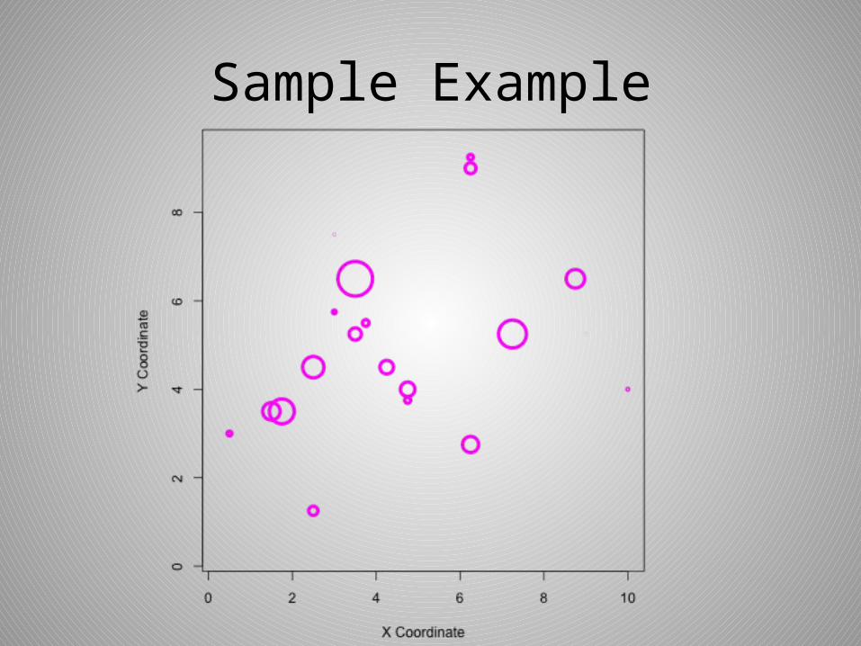
Sample Example

Geostatistics: The Procedure Theoretical

• Ordinary Kriging: “Best Linear Unbiased Estimator”• Attempts to minimize the variance of the errors, estimates

using weighted linear combinations, and attempts to have the mean residual equal to zero (Isaaks 278).

• Rough procedure derivation: (1) Use a random function model for each point of estimation, (2) Ensure that the expected value of the error at any particular location is zero (unbiasedness), (3) Use partial derivatives to minimize the variance of the model error using the constraint that the weights sum to one, to do this we must introduce a Lagrange parameter, (4) Solve a large system of equations (Isaaks 279-288).

Geostatistics: The ProcedurePractical

• Now as the user, we must choose a covariance function to calculate the covariance between all sample locations and with the point we are interested in estimating. Along with the previous derivation, this allows us to find the weights we desire to have for making our estimation (Isaaks 287-289).

• This can be repeated several times to make estimates at many locations and create a contour map of concentrations, for example.

Contour map example

Geostatistics: The ProcedureReally Practical: Choosing the Variogram and Covariance Model

• Take samples over region.• Determine empirical semi-variogram. To find the semi-variance: At

a given distance, calculate the sum of the square differences of all data points at that distance apart, and divide by twice the number of pairs (Clark Chapter 2).

• Plot the semi-variance vs. distance (empirical semi-variogram). • Choose a variogram model. Most interested in fitting small

distances. Several models to choose from with particular characteristics. Note: variogram model selection determines covariance model.

• Fit variogram model to data. Now we have a model estimating the relationship (similarity) of data values at locations of varying distance! Yippee!

Empirical semi-variogram example

My Objectives

• Focus on sample size and model fitting, rather than global prediction and mapping.

• Explore the effect of sample size on the accuracy of a fitted model.

• How do different models (other than the one used to simulate the data) fit data sampled from the simulation.

• What effect does shifting the data locations have on fitting a model.

• Keep in mind that I always created new simulations.

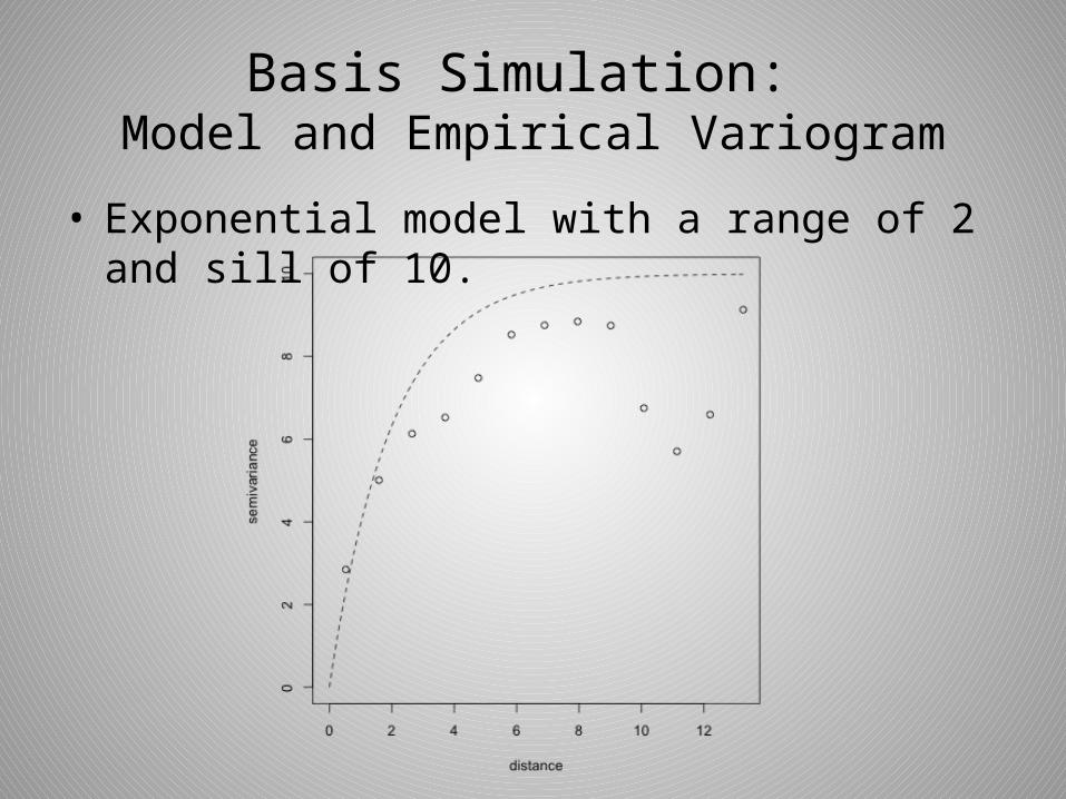
Basis Simulation: Model and Empirical Variogram

• Exponential model with a range of 2 and sill of 10.

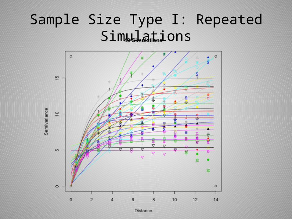
Sample Size Type I: Repeated Simulations

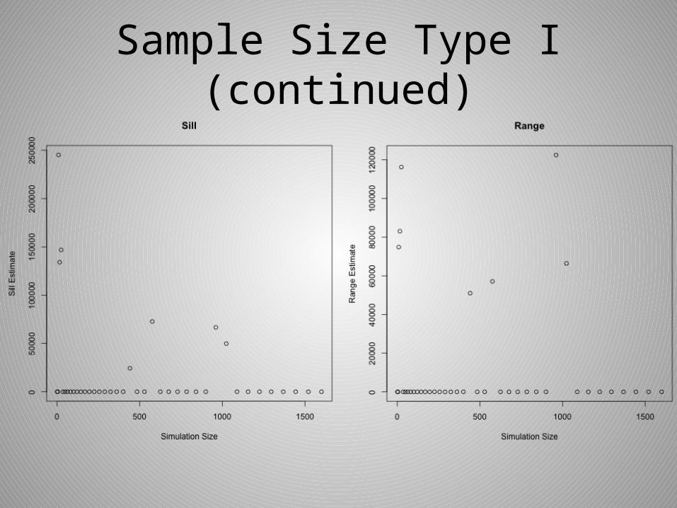
Sample Size Type I (continued)

Sample Size Type I: Repeated Sampling, analyzing Sill and Range

• Most often it was the simulations of smaller sizes that behaved undesirably, but it is worth noting that this was not always the case.

• After realizing that repeated simulations were not very practical, I took samples of varying size from one simulation and attempted to analyze the sill and range estimates.

• The results were better, but there were still often outliers that made comparing the estimates difficult.

• I moved on to considering function values. From here on out all my samples are simple random samples.

Sample Size Type II: Function Values

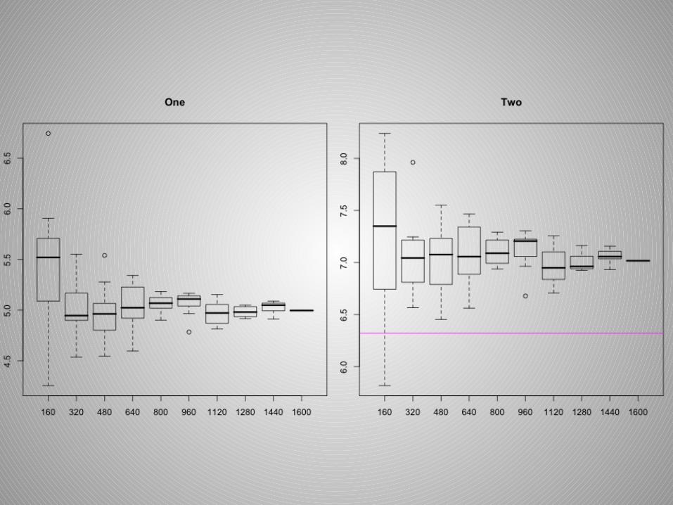
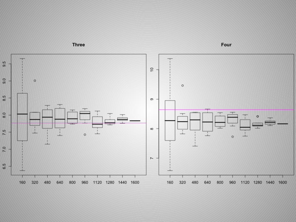
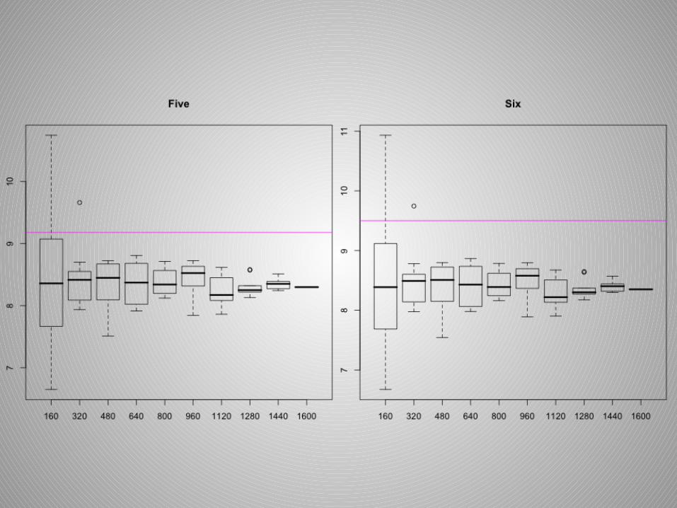
Thoughts on Sample Size

• Comparing sill and range estimates is not very useful when creating several simulations or taking samples.

• I decided a sample size of 640 to 800 out of 1600 is adequate. A great deal more of precision is not gained taking more data points.

• I took samples of size 700 for each of the rest of the explorations.

Fitting Other Models

Model Selection• Note that this example worked out particularly

nice, but often one or more of the models didn’t fit in a meaningful way.

• I found there to be 3 types of models that I considered, broken down in this way:– Linear– Wave, Gaussian, Cubic, Cauchy– Exponential, Spherical

• Trying to fit data outside of its ‘type’ will likely be unsuccessful.

Shifting Data Point Locations

Shifted Data Points: The Fitted Models

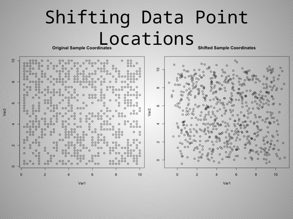
Shifting Data Point Locations

• Used random standard normal values to shift each data point’s location.

• I noticed that I had to ‘mess’ up the locations quite a bit before seeing a real difference in the fitted variogram models.

• This example had a mean location shift of 0.620 units. Pretty large in a 10x10 square unit grid.

Closing Remarks

• On sample size, model fitting, and shifting data locations.

• Do differently: Nothing. No regrets. Just kidding. Looking back, I would analyze the sample size results more.

• In the future: Work more with practical data sets, analyzing observed data.

Citations

• Advisor: Ron Barry, Professor of Statistics• Clark, Isobel. Practical Geostastics. 1979. Viewed online April

2010. http://www.kriging.com/PG1979/ • Issaks, Edward H., and R. Mohan Srivastava. An Introduction to

Applied Geostatistics. New York: Oxford University Press, 1989.