Advisor: Dr. Askar Choudhury, Mr. James Jones ,and Dr. Krzysztof M. Ostaszewski

2011

ISU/MAT Zhongkai Wen

EXPLAINING MAIZE PRICE IN NORTHERN

REGION OF GHANA BY LINEAR

REGRESSION MODEL

Contents

Abstract ......................................................................................................................................................... 1

Introduction .................................................................................................................................................. 2

Objective ....................................................................................................................................................... 7

Methodology ................................................................................................................................................. 8

Results and Discussion ................................................................................................................................ 11

Northern region ...................................................................................................................................... 11

Upper East region ................................................................................................................................... 13

Upper West region .................................................................................................................................. 15

Conclusion ................................................................................................................................................... 16

Reference .................................................................................................................................................... 16

Appendix ..................................................................................................................................................... 18

Variable lists ............................................................................................................................................ 18

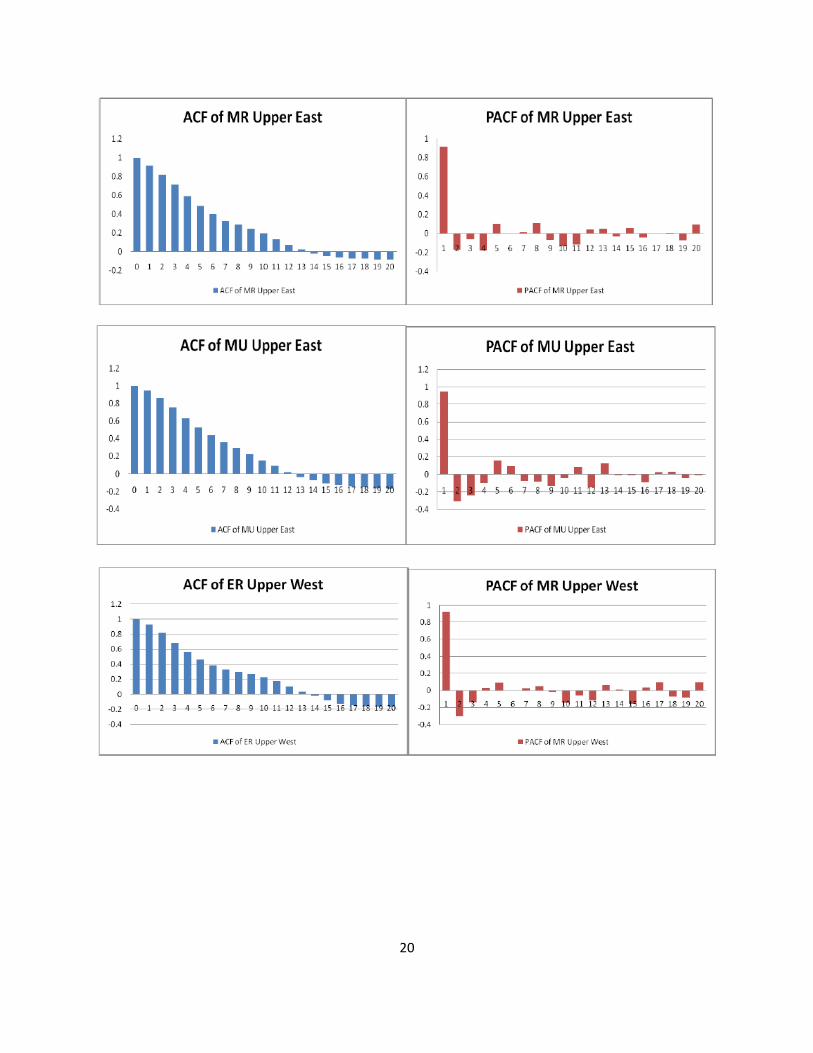
Charts of ACF and PACF for different regions ......................................................................................... 19

1

Abstract: In this project, the price of maize from three northern regions (northern

region,uppereast region and upperwest region) was investigated. Regression analysis

was done to fit the price data with proper linear model.The linear model was identified

through the cycle of autocorrealtion check, stepwise method and nomality check .Finally

Logarithm tranforamtion of price data was chosen to make the linear regression residual

normally distributed and stable.The linear regression results of logarithm transform

showed positive correlation between the price of maize and price of rice in all three

regions,which is different from expectation.It also shows that the price is correlated with

the harvest season, however,which varies for different regions.

2

Introduction

Farming is a major source of income for many people in developing countries. In Ghana

it represents 36 percent of the country’s GDP and is hiring more than 50 percent of the

population ( Lisa Biederlackand Jonathan Rivers,2009). Agricultural production depends

on a number of factors including economic, political, technological, as well as factors

such as disease, fires, and certainly weather. As a consequence of climate change,

agriculture in many parts of the world has become a riskier business activity. Given the

dependence on agriculture in developing countries, this increased risk has a potentially

dramatic effect on the lives of people throughout the developing world especially as it

relates to their financial inclusion and sustainable access to capital. It’s very important to

develop some insurance products to protect crop producers from such risks.Price of

crops is very important factor in farming industry and predicting price will help farmers

reduce the loss from weather changes.

The agribusiness has become very complex in recent years, and hence the importance

of agricultural planning has increased. Crop producers can often base their decisions for

crop production and selling on yield and price forecasts. Prediction of future crop selling

prices is another important aspect in decision planning. Accurate price predictions will

help in planning what crops to be planted and when to sell them to optimize the overall

profit. Consequently, a crop price forecasting model for predicting the upcoming prices

in any specific location and at aggregation level (e.g. weekly) will help local farmers to

optimize their crop selling strategy( Nantachai Kantanantha ,Nicoleta Serban,and Paul

Griffin).

Predicting prices for food staples in poor regions is crucial for combating food insecurity,

defined as the ability to purchase enough food to lead an active and healthy life. Food

insecurity is most frequently caused by insufficient access to food instead of absolute

lack of food availability. In Ghana, with its large population of poor who spend over half

their income on food, the local price of food can be a significant source of food

insecurity(Molly E. Brown ,Nathaniel Higgins , and Beat Hintermann,2009).

3

A number of models have been developed to forecast the cash prices. Kenyon and

Lucas (1998) study the relationship between soybean season average prices and

soybean ending stocks - the difference between supply and demand. They propose a

simple price forecasting model using price historical data and the ending stocks based

on linear regression. Many researchers studied the role of futures contract prices in

agricultural price forecasting (Working, 1942; Tomek and Gray, 1970,Kenyon et al.,

1993). Futures’ price is often used as an indicator of the expected cash price (Hoffman,

2005). Eales et al. (1990) examine the difference between futures prices and the

average cash prices surveyed from farmers and grain merchandisers in Illinois. In most

cases, futures’ price and cash price are not significantly different. Because the futures

crop price is an indicator of the cash price behavior. Zulauf and Irwin conclude that

marketing strategies offer little hope of increasing returns over simply selling at harvest.

They suggest that, because futures are efficient, the futures market should be used as a

source of information rather than as a trading medium. Kastens, Jones and Schroeder

compared various simple-to-construct forecasting methods for cash prices and

concluded that the deferred futures plus historical basis forecast method was the most

accurate for most commodities considered. Brorsen and Irwin suggest that, rather than

forecasting prices, extension economists should rely on the futures market to provide

the price forecasts needed in outlook programs. Kastens and Dhuyvetter looked at

incorporating deferred futures prices and historical localized basis to make grain storage

decisions. However, positive returns to storage were not generally found, indicating that

cash markets appear to be efficient.

Crop production flexibility today requires producers to make management decisions

based on market conditions. Economically sound decisions are critical for producers to

manage risk and take advantage of marketing opportunities. An integral factor in

production and marketing plans is accurate forecasting of the local crop basis.

In the agribusiness literature, commodity basis is denoted as the difference between the

local market cash price and the price of a futures contract for a specific time period.

Being able to accurately predict basis is critical for making marketing and management

4

decisions. Basis forecasts can be used along with futures prices to provide cash price

projections(Mykel Taylor,Kevin C. Dhuyvetter,and Terry L. Kastens,2004).

Typically, basis forecasts are based on simple time series or naive models. That is,

expected (future) basis is assumed to be historical basis. Nonetheless, especially

complex models for forecasting basis are probably not relevant for producers, as

producers must be able to constantly and quickly translate futures prices to cash price

expectations for such information to be useful. Moreover, structural models requiring

ancillary forecasts of explanatory variables are of little value to producers needing to

make production decisions based on price forecasts with limited information available.

Many studies have examined factors affecting basis. Studies have shown basis

forecasts based on simple historical averages compare favorably with more complex

forecasting models.

A fundamental structural model incorporating storage cost, transportation cost, and

regional supply and demand variables is developed to explain basis behavior( Bingrong

Jiang and Marvin Hayenga).

Dhuyvetter and Kastens built upon previous work by Hauser, Garcia, and Tumblin by

comparing practical methods of forecasting basis for wheat, corn, milo, and soybeans in

Kansas. They found that a 4-year historical average was the optimal number of years to

forecast basis. A longer-term average (5 to 7 years) was optimal for corn, milo, and

soybeans. They looked at incorporating current market information into forecasts using

futures price spreads and an historical average that is adjusted by current nearby basis

information. The basis forecasts were slightly more accurate when incorporating price

spreads between futures contracts than using current nearby basis information.

However, neither of these methods was better than a simple historical average with time

horizons greater than 8 to 12 weeks. This analysis did not recognize that the optimal

amount of current information to incorporate, when adjusting an historical average, is

likely a function of the time horizon. Incorporating current market information, such as

current nearby basis deviation from an historical average, into a harvest basis forecast

improves accuracy for only the 4 weeks ahead of harvest vantage point, but improves

5

the accuracy of post-harvest basis forecasts (24 weeks after harvest) from nearly all

vantage points considered (Scott W. Barnhart,1989).

Technological change has transformed agriculture in the US, Europe and large parts of

Asia and South America, but it has largely bypassed West Africa. In this region, most

farms are small, primarily cultivated with hand tools, planted with seeds with a low yield

potential, using little or no chemical or organic fertilizer. The climate is arid or semi-arid,

and there is inadequate infrastructure to provide water for irrigation. Consequently, most

small farms are only able to attain yields which are less than one seventh of those

regularly achieved in industrialized systems (Breman, 2003; Taylor et al., 2002).

Agriculture in northern Ghana remains particularly vulnerable. For example, the average

range of district-level maize yields in the north from 1992 to 2005 was 35 percent higher

than in the forest and 55 percent higher than at the coast. Higher rates of rural poverty

are likely exacerbated by factors linked to fewer opportunities for intensifying and

commercializing agriculture, such as poorer access to input and output markets as well

as credit and advisory services. Concerns about food insecurity are likely to remain

greater in the north, and such concerns may influence farmers to choose production

strategies that minimize risk rather than maximize comparative advantages for market

opportunities. Ghanaian agriculture is overwhelmingly dominated by smallholders; many

commodities—including cocoa, maize, and cassava—are produced predominantly on

small farms. More than 70 percent of Ghanaian farms are 3 hectares (ha) or smaller in

size (Chamberlin 2007). The smallest average holdings are in the south (for example,

2.3 ha at the coast versus 4.0 ha in the northern savanna). Smaller farms tend to

produce fewer commodities; for example, farms of 2 ha or smaller produce an average

of 3.1 crops; whereas those of 4 ha or larger produce 4.7 crops, on average. Maize and

cassava are particularly important crops for the smallest farms, reflecting the

importance of these crops to food security strategies under poor or variable market

conditions. (For the 12 percent of households that grew only these two crops, the

median holding size was 0.8 ha.)

6

Smallholder market participation rates vary by holding size. Smaller farms produce

fewer marketed crops and are less likely to sell the crops they do produce. Participation

also varies with geography. The marketed share of farm products and the percentage of

farmers who sell their produce tend to be lowest in northern Ghana Holding sizes

increase from south to north, but this increase is accompanied by lower land

productivity in the north. At the same time, land endowments are more important to farm

livelihood strategies in the north, where larger holding sizes correspond to higher

household incomes. This finding appears to indicate that efforts to increase farmer

incomes should particularly emphasize land productivity in the north, where fewer off

farm opportunities exist (Small holder agriculture in Ghana).

In Ghana, due to insufficient storage and drying facilities and lack of credit, a lot of

farmers are obliged to sell their products at post harvest time when prices are low and

re-buy during the lean season when prices are high. For example of the millet in the

nearby area of Ghana, there is a widespread lack of storage facilities (Dembele and

Staatz, 1999). Because they cannot store grains for an entire year, small farmers sell

more than their surplus (defined by total output minus annual consumption) on the

market after harvest and buy some grain back later in the year, often at higher prices.

Because of the simultaneous influx of grain, prices drop to their base levels after

harvest. As producers draw down their stocks, supply on the market decreases,

whereas consumer demand remains unchanged, leading to a gradual increase of millet

prices during spring. During the ―hungry season‖ in summer, many farmers become net

millet buyers because their own stocks are depleted, further boosting prices (Cekan,

1992). Annual prices peak just before harvest, the time of which differs across climate

zones, which is the reason for the different price peaks in Niger on the one hand (July)

and Burkina Faso and Mali on the other (August) (Molly E. Brown ,Nathaniel Higgins ,

and Beat Hintermann,2009).

The combination of limited income opportunities with high dependence on markets for

food purchases, rural households’ purchasing power is stretched which in turn is likely

to negatively impact on the quality and quantity of food they consume. Market centres

7

for food are not well integrated into rural areas because of limited road access, poor

road conditions, a one-way trade direction from traders to communities. This one-way

trade direction compensates for the communities’ limited access to markets but

transaction costs tend to be high, which further constrains the already limited

purchasing power of the rural population living in remote areas (Lisa Biederlack and

Jonathan Rivers,2009).Knowing the trend of crop price is very important for the farmers

to manage their productions and manage their income distributions. Northern regions of

Ghana are the poorest parts of Ghana. Such crop price information will be of much

more importance to the farmers in these regions.

Based on the reference papers and the actual data we got for Ghana, in this project,

first we try to explain the maize price in these regions. Because farmers in northern

region don’t have many storage facilities and the trade of the crops are not far away

from their hometown because of poor road system in northern region. The northern

region, the trading is not affected much by the international markets. In Ghana’s case,

the time series linear regression model will be used to find the relationship among

monthly maize price, monthly rice(food substitute for maize) price with consideration of

seasonality(i.e. harvest season and non-harvest season) . The maize price lags are

included in price forecasting models because there is a number of price drivers that are

important but typically unobserved. In this case, these unobserved price drivers include

income, distribution bottlenecks, local price-related policies, price expectations by

farmers and consumers, and the quality of agricultural land. Some of these unobserved

price determinants tend to move slowly over time. Lagged dependent variables on the

right-hand side of a price equation capture these unobserved, autocorrelated price

drivers. We control for the cyclical behavior of prices by introducing monthly dummy

variables.

Objective

Crop Price is an important factor for developing crop-realted insurance products.In the

project, first, I will try to explain maize price using linear model. The seasonality and

8

maize substitute(rice) will be included as predictors.The model was shown as following.

F() stands for some possible transformation of dependent time series variables.

F(Mrt)=β0+β1*rlr+Σαi*month+Σγi*f(Mr(t-i))+Σδi*year

Based on the model developed in the first step; try to do some forcasts of the price.

Hypothesis:The crop price is linear related with predictors shown above.

Based on this assumption, I did regression alalysis on these data.

Methodology

In order to determine the factors that influence maize price in these regions, since they

are time series data sets, auto regression checks were done to test the autocorrelation

between the lags of maize price. In SAS, the ARIMA procedure was used to get ACF

and PACF charts.Based on the ACF and PACF, the order of autoregression was

identified. By looking at the autocorrelation function (ACF) and partial autocorrelation

(PACF) plots of the series, we can tentatively identify the numbers of AR and/or MA

terms that are needed. ACF plot is a bar chart of the coefficients of correlation between

a time series and lags of itself. The PACF plot is a plot of the partial correlation

coefficients between the series and lags of itself. A partial autocorrelation is the amount

of correlation between a variable and a lag of itself that is not explained by correlations

at all lower-order-lags. The autocorrelation of a time series Y at lag 1 is the coefficient of

correlation between Y(t) and Y(t-1), which is presumably also the correlation between

Y(t-1) and Y(t-2). But if Y(t) is correlated with Y(t-1), and Y(t-1) is equally correlated with

Y(t-2), then we should also expect to find correlation between Y(t) and Y(t-2). The

partial autocorrelation at lag 2 is therefore the difference between the actual correlation

at lag 2 and the expected correlation due to the propagation of correlation at lag 1. The

partial autocorrelations at all lags can be computed by fitting a succession of

autoregressive models with increasing numbers of lags. In particular, the partial

autocorrelation at lag k is equal to the estimated AR(k) coefficient in an autoregressive

model with k terms--i.e., a multiple regression model in which Y is regressed on

LAG(Y,1), LAG(Y,2), etc., up to LAG(Y,k). Thus, by mere inspection of the PACF we

9

can determine how many AR terms you need to use to explain the autocorrelation

pattern in a time series: if the partial autocorrelation is significant at lag k and not

significant at any higher order lags--i.e., if the PACF "cuts off" at lag k--then this

suggests that you should try fitting an autoregressive model of order k .In the case of

maize price of Ghana in three northern regions , the PACF plot has a significant spike

only at lag 1, meaning that all the higher-order autocorrelations are effectively explained

by the lag-1 autocorrelation. It has a very large spike at lag 1(showed in the following

figure) and no other significant spikes, indicating that in the absence of differencing an

AR(1) model should be used.

Figure1 ACF and PACF bart chart of maize price of northern region in Ghana.

Stepwise method was used to identify independent variables. The significance level of

antry and stay of stepwise method was set at 10%.Based on the stepwise method,

independent variables were chosed for the regression analysis.Auto regression

procedure with maximum likelihood method was used to determine the linear regression

model based on the variables identified in the previous steps. The residual was

obtained through this step and the stationarity and normality of residue were checked

using univariate procedure in SAS.If non-normally distributed data was observed based

on the Kolmogorov-Smirnov test, certain transformations(including difference and

logarithm) of dependent variable were done to make sure the residual was normally

distributed, In this project, the natural logarithm transformation was used to improve the

normality of the data.Then again back to the first step, the autorecorrealtion of the

10

transformation was checked through ACF and PACF until the proper order of

autoregression was applied(the ACF and PACF bart charts of logarithm transformation

were shown below. The ACF and PACF charts still indicated the first order of

autoregression.The ACF and PACF bar charts of first difference showed no significant

autocorrelation. ).

Figure2 ACF and PACF bar charts of logarithm transformation of maize price of

northern region

Firgure3 ACF and PACF bar charts of first difference of maize price of northern region

Even though the first difference showed no significant autocorrelation, the logarithm

transformation was applied .Because the logarithm transformation made the residual of

regression model normally distributed and stable(especially for the maize price data of

northern region and upper west region of Ghana),which is basic assumption the

statistics test can be used to check the significance of coefficents of regression

11

models.When the first lag of regression was included as a predictor in the regression

model, the residual showed normality and showed no significant autocorrelation

anymore.The logarithm transformation was finally chosen in the regression analysis.The

logarithm form also gave the approximate quantity of percent change in depend variable

(here, it is the percentage of change in price).

Results and Discussion

Northern region

The autocorrelation was checked in the orignial form of maize price data,first difference

and natural logarithm form of price data.The ACF of original maize price showed strong

but decreasing correaltion between different lags and PACF of it showed only one

strong spike at lag1,which suggests a first order correlation. The linear regression was

run through the autoregression procedure with first lag of maize price as one of the

predictors in the model.The regression model with coeffiicents is as following:

MRt=1.9436+0.6310MR(t-1)+0.1072RLR+3.2306JUL-0.7345OCT-

0.9213Year2003+2.0241year2005+7.1917Year2008+Vt(R-square=0.8718)(1)

Vt=-0.4481V(t-1)+ᵋt

The normality of residual from this regression model was checked .The Histogram and

Q-Q probability plot showed lack of enough normality.The P-value of Kolmogorov-

Smirnov test is less than 0.01, which confirmed the lackness of normality.

-8 -6 -4 -2 0 2 4 6

0

10

20

30

40

50

60

Pe

rce

nt

res 0.1 1 5 10 25 50 75 90 95 99 99.9

-7.5

-5.0

-2.5

0

2.5

5.0

7.5

res

res

Normal Percentiles

Fuigure4 histogram and Q-Q plot of residual of model(1)

12

The results above showed the lackness of normality. So certain transformation of the

maize price should be done to reduce this non-normality.The logarithm form of maize

price was chosen to increase normality.The same routine was used to check the

logarithm form.The ACF and PACF showed in figure2 suggests the first order

autoregressin model.So the first lag of logrithm form was included in the model.The

similar autoregression procedure was used to fit the data. The regression results

showed as following:

LOGMRt=0.6563+0.7086LOGMR(t-1)+0.0048RLR-0.1844SEP-0.1453OCT-0.0496NOV-

0.0503Year2003+0.0813year2005+0.1404Year2008+Vt(R-square=0.8718)(R-sqr:0.9203)(2)

Vt=--0.3088V(t-1)+ᵋt

The autocorrelation was checked for the residual from the model above.The ACF and PACF showed no significant autocorrelation.The bar chart of PACF showed no

significant autocorrelation.

Figure4 ACF and PACF of residual of regression

Variable DF Estimate Error t Value Pr > |t|

Intercept 1 0.6563 0.2354 2.79 0.0069

lglogmr 1 0.7086 0.0998 7.10 <.0001

rlr 1 0.004808 0.001749 2.75 0.0076

Sep 1 -0.1844 0.0420 -4.39 <.0001

Oct 1 -0.1453 0.0451 -3.22 0.0019

Nov 1 -0.0496 0.0434 -1.14 0.2569

2008 1 0.1404 0.0704 1.99 0.0500

2005 1 0.0813 0.0509 1.60 0.1147

2003 1 -0.0503 0.0486 -1.04 0.3043

AR1 1 -0.3088 0.1744 -1.77 0.0810

13

The normality of the residual was checked through the univariate procedure in SAS.The

histogram and the Q-Q probability plot showed the normality.This is confirmed by the

Kolmogorov-Smirnov test (P-value=0.15).

-0.24 -0.16 -0.08 0 0.08 0.16 0.24

0

5

10

15

20

25

30

35

40

45

Pe

rce

nt

res 0.1 1 5 10 25 50 75 90 95 99 99.9

-0.3

-0.2

-0.1

0

0.1

0.2

0.3

res

res

Normal Percentiles

Firgure5 Histogram and Q-Q plot of residual

All these checks indicated that the linear regression model of logarithm transformation

was a good model for the price data.The significance of the coefficients of september

and october dummy variables corresponded to low price in the harvest season of maize.

The negative coefficients can be explained by the fact that after the harvest season the

price will drop. The coeffient of september is less than that of october, which means the

price in september dopped more than in october.The positive and significant relation

with rice price means that the rice price and maize price will rise simutaneously however

with different amount, which is not as expected. Because rice is a subsitute for maize, I

expect negative relationship between these two prices.The positive relation might be

from the lack of enough of supply of staples in the market.The significance of the first

lag shows that the lag of price is a good expectation for the price of next duration.

Upper East region

The same procedure was done for the data from upper east region.Following was the

result for linear regression .The R-square of the regression model is 0.8139.The ACF

and PACf of the residual showed no significant auto correlation.The P-vale of

Kolmogorov-Smirnov test is 0.065.The histogram and Q-Q plot of regression residual

indicated that the transformation made the residual close to normally distribution.

14

Figure6 ACF and PACF chart for residual of logarithm transformation regression.

-0.18 -0.12 -0.06 0 0.06 0.12 0.18 0.24

0

5

10

15

20

25

30

35

40

Pe

rce

nt

res

0.1 1 5 10 25 50 75 90 95 99 99.9

-0.3

-0.2

-0.1

0

0.1

0.2

0.3

res

res

Normal Percentiles

Figure 7Histogram and Q-Q plot of regression residual.

The significance of month July with positive coefficient corresponded to higher the pre-

harvest price than other season.The significant positive relation between maize price

and rice price can be explained by the same reason for the northern region,i.e. lack of

enough supply of staples in this region.

Variable DF Estimate Error t Value Pr > |t|

Intercept 1 0.7479 0.3371 2.22 0.0296

lglogmu 1 0.6797 0.1311 5.19 <.0001

rlu 1 0.003633 0.001577 2.30 0.0241

Jul 1 0.0700 0.0250 2.81 0.0064

2005 1 0.0526 0.0527 1.00 0.3215

2008 1 0.1536 0.0745 2.06 0.0427

AR1 1 -0.6627 0.1731 -3.83 0.0003

15

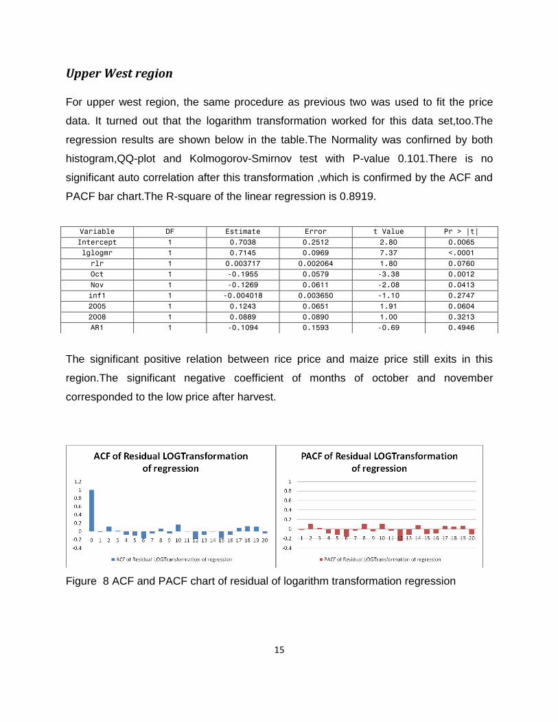
Upper West region

For upper west region, the same procedure as previous two was used to fit the price

data. It turned out that the logarithm transformation worked for this data set,too.The

regression results are shown below in the table.The Normality was confirned by both

histogram,QQ-plot and Kolmogorov-Smirnov test with P-value 0.101.There is no

significant auto correlation after this transformation ,which is confirmed by the ACF and

PACF bar chart.The R-square of the linear regression is 0.8919.

The significant positive relation between rice price and maize price still exits in this

region.The significant negative coefficient of months of october and november

corresponded to the low price after harvest.

Figure 8 ACF and PACF chart of residual of logarithm transformation regression

Variable DF Estimate Error t Value Pr > |t|

Intercept 1 0.7038 0.2512 2.80 0.0065

lglogmr 1 0.7145 0.0969 7.37 <.0001

rlr 1 0.003717 0.002064 1.80 0.0760

Oct 1 -0.1955 0.0579 -3.38 0.0012

Nov 1 -0.1269 0.0611 -2.08 0.0413

inf1 1 -0.004018 0.003650 -1.10 0.2747

2005 1 0.1243 0.0651 1.91 0.0604

2008 1 0.0889 0.0890 1.00 0.3213

AR1 1 -0.1094 0.1593 -0.69 0.4946

16

-0.42 -0.30 -0.18 -0.06 0.06 0.18 0.30 0.42

0

5

10

15

20

25

30

35

40

Pe

rce

nt

res

0.1 1 5 10 25 50 75 90 95 99 99.9

-0.6

-0.4

-0.2

0

0.2

0.4

res

res

Normal Percentiles

Figure 9 Histogram and Q-Q plot of residual

Conclusion

The regression analysis of three regions has similar results, the harvest season effect

showed in all three linear regression models, even if the effect showed significant in

different months.They have positive effect before harvest season and negative effect

after harvest season.The positive relationship between rice price and maize price

showed in all three models. This might be explained by the lack of supply of both of

them.

Reference

Acquah, Henry De-Graft (2010) .Asymmetry in Retail-Whole sale priceTransmission for

Maize:Evidence from Ghana.American-Eurasian J.Agric.&Environ.Sci.,7(4):452-456.

Armath, Paul W. and Felix Asante(2006).Traditional Maize Storage Systems and

Staple-Food Security in Ghana.Journal of Food Distribution Research 37(1),40-45.

Barnhart, Scott W. (1989).The Effects of Macroeconomic Announcements on

Commodity Prices.American Journal of Agricultural Economics, Vol. 71, No. 2 (May,

1989), 389-403.

Biederlack,Lisa (WFP) and Jonathan Rivers (WHO) (2009).Comprehensive Food

Security & Vulnerability Analysis (CFSVA) Ghana,April, 2009 .

Brandt, Jon A. and David A. Bessler(1982). Forecasting with a Dynamic Regression

Model: A Heuristic Approach. North Central Journal of Agricultural Economics, Vol. 4,

No. 1 (Jan., 1982), 27-33.

17

Brown, Molly E. , Nathaniel Higgins , and Beat Hintermann(2009) .A Model of West

African Millet Prices in Rural Markets. CEPE Working Paper No. 69 ,November 2009.

Cromarty,W. A. (1961).Free Market Price Projections Based on a Formal Econometric

Model .Journal of Farm Economics, Vol. 43, No. 2 (May, 1961), 365-378. [5]

Elmer,J.(1930). Evaluation of Methods Used in Commodity Price Forecasting.Journal of

Farm Economics, Vol. 12, No. 1 (Jan., 1930), 119-133.

Jiang,B.,and M.Hayenga.(1997). Corn and Soybean Basis Behavior and Forecasting:

Fundamental and Alternative Approaches.Proceedings of the NCR-134 Conference on

Applied Commodity Price Analysis, Forcasting, and Market Risk

Management.Chicago,IL.

Kantanantha,Nantachai, Nicoleta Serban,and Paul Griffin .Yield and Price Forecasting

for Stochastic Crop Decision Planning.

Lopatka, Jessica,Jason Topel, and Pedro de Vasconcellos(2008). Food Staples in the

Ghana School Feeding Program: Analysis of Markets, Value Chains, and Menus. UC

Berkeley – Haas School of Business International Business Development Program [23]

Micro Insurance in Africa: Filling the Distribution Gap. 3 rd African Microfinance

Conference, August 20‑23, 2007

Minot , Nicholas and Reno Dewina (2010).Impact of food price changes on ousehold

welfare in Ghana. International Food Policy Research Institute Prepared for the U.K.

Department for International Development under the project ―Assessing Impact of

Increased Global Food Price on the Poor‖

Pettee, E. W. (1936). Short-Term Price Forecasting 1920-29. The Journal of Business

of the University of Chicago, Vol. 9, No. 3 (Jul., 1936), 280-300.

OWUSU ,Frank Kofi (2010). Time Series ARIMA Modelling of Inflation in Ghana: (1990

– 2009).Thesis for master degree.

Sarris, Alexander (2002). The Demand for Commodity Insurance by Developing

Country Agricultural Producers: Theory and an Application to Cocoa in Ghana. World

Bank Policy Research Working Paper 2887, September 2002.

18

Shively, Gerald E. (1996). Food Price Variability and Economic Reform: An ARCH

Approach for Ghana. American Journal of Agricultural Economics, Vol. 78, No. 1 (Feb.,

1996), 126-136.

Shonkwiler, J. S. and G. S. Maddala(1985). Modeling Expectations of Bounded Prices:

An Application to the Market for Corn.The Review of Economics and Statistics, Vol. 67,

No. 4 (Nov., 1985), 697-702.

Skees, Jerry R., J. Roy Black, Barry J. Barnett(1997). Designing and Rating an Area

Yield Crop Insurance Contract. American Journal of Agricultural Economics, Vol. 79, No.

2 (May, 1997), pp. 430-438

Small holder agriculture in Ghana. International food policy research institute

Swamikannu ,Nedumaran, Felix Asante, Schreinemachers Pepijn and Thomas

Berger(2007). Food Consumption Behavior of Ghanaian Households: A Three-Step

Budgeting Approach. Documentation of Research.

Taylor, M., Kevin C Dhuyvetter, and Terry L. Kastens(2004). Incorporating Current

Information into Historical-Average-Based Forecasts to Improve Crop Price Basis

Forecasts.Paper presented at the NCR-134 Conference on Applied Commodity Price

Analysis,Forecasting, and Market Risk Management,St. Louis, Missouri, April 19-20,

2004

Working ,Holbrook (1958). A Theory of Anticipatory Prices, The American Economic

Review, Vol. 48, No. 2, Papers and Proceedings of the Seventieth Annual Meeting of

the American Economic Association (May, 1958), pp. 188-199

Yilma ,Tsegaye (2006). Market Survey in the Upper East Region of Ghana. Josef G.

Knoll Visiting Professorship for Development Research.

Appendix

Variable lists

MR-maize price rural monthly

19

LOGMR: logarithm of maize price

LGLOGMR: first lag of logmr

MU:maize price urban monthly

RLR:local ricew rural monthly

RLU:local rice urban

(All the price data was converted to new Ghana cedi.)

IINF1:inflaion rate*100

FEB-DEC:month dummy variables with value 0 and 1.

2002-2008-year dummy variables with value 0 and 1

UW,UE,NR-area dummy variables with value 0 and 1 .UW-upper west,UE-upper

east,North region

AR1:autoregression with order 1

Data was collected from year 2002 to 2008.All the price data was provided by

department of Statistics in Ghana.

Charts of ACF and PACF for different regions

20

21