estimation of the oil production potential of...
TRANSCRIPT
ESTIMATION OF THE OIL PRODUCTION POTENTIAL OF THE FIELD SINGUE, ORIENTE BASIN, ECUADOR
GUILLERMO FERNANDO GUERRA DEL HIERRO
MSc
School of Computing Science and Engineering
University of Salford
This dissertation is submitted in part fulfilment of the requirements
for the MSc degree in Petroleum and Gas Engineering
SUPERVISOR: MR ALLAN WELLS
2014

ii
DECLARATION
“I, GUILLERMO FERNANDO GUERRA DEL HIERRO, declare that this dissertation is
my own work. Any section, part or phrasing of more than 20 consecutive words that is
copied from any other work or publication has been clearly referenced at the point of use
and also fully described in the reference section of this dissertation.”
“Signed ………………………………………..”

iii
CERTIFICATION
“I certify that I have read this report and in my opinion it is fully adequate in scope and
quality, as partial fulfilment of the degree of Master in Science in Petroleum and Gas
Engineering.”
“Signed ………………………………………………”
MR. ALLAN WELLS
SUPERVISOR

iv
ABSTRACT
The Oriente Basin is the most important oil reservoir in Ecuador. The field Singue is one of the oil fields that is located in the basin and is considered to be one of the marginal fields of the region that have not been developed yet. In the area of the field there is one abandoned well called Singue-1 and other dry well called Alama-1. The Oriente Basin has from deep to top the following formation rocks: Hollin, Napo, Tena, Tiyuyacu, Orteguaza, Chalcana, Arajuno and Chambira. The present study is done on the Napo sandstones of the field Singue.
The objective of the project is to estimate the oil production potential of the field reservoirs based on the analysis of well logs, seismic data and background information of the basin across the region. Napo is a sandstone reservoir with high possibilities of oil production. It is subdivided in lithofacies whithin these are the sandstones: U up, U low, T up, T low and Basal T. Analysis of well logs is performed to identify the lithofacies and to calculate the petrophysical properties of each rock component. Seismic interpretation of the region is done to identify the boundaries of the reservoir. Reserves estimations are performed by the volumetric method on the net pay zones for each formation.
Based on calculations performed on the net pay interval, Napo U low is the facie that has the highest potential of oil content followed by Napo T up, Napo Basal and Napo U up. In the area of the field there are two major faults and the oil trapping structure is an anticline. The final results of the oil reserves in Napo U low sandstone are 3,270,746 bbl. and reach up to 8,065,545 bbl. if all the facies are considered.

v
DEDICATION
This work is dedicated to my family for all the support,
And to the people that believe in education as a key force to improve the world.

vi
ACKNOWLEDGEMENT
Thanks to God for all his blessing and to my family for their unconditional support.
Especially thanks to my sponsor SENESCYT in behalf of the government of Ecuador that
is promoting the scholarship program, believing in education as the main resource for the
development of the country.
The project is structured to complete the MSc. Petroleum and Gas Engineering program.
This work was completed under the tutelage of Mr. Allan Wells, scholar at the Petroleum
at Gas department of the University of Salford, would like to thank my supervisor who has
delineated and supervised the development of this project. In addition, would like to thank
all the staff and lecturers of the University of Salford that have contributed to enhance my
knowledge during this last year of study, especially to Dr. Lateef Akanji, the coordinator of
the Petroleum department and mainly Petroleum lecturer, who also has supported me with
the technical assessment for this project, as well as to Mr. Abubakar Abbas, as passionate
lecturer and technical advisor.
Additionally, would like to thank the personnel of Dygoil Cia Ltda, Ecuadorian company
who provided information for the development of the thesis. Thanks to them I discovered
the world of oil and the importance of promoting domestic industry so I decided to study
this program, thanks for the on-going technical support.
Finally would like to thank the support and encourage of my friends, especially the ones
who have meet during this year and have collaborated with their knowledge related to this
project.
The author recognizes that there are still some shortcomings in the development of the
project. Any suggestion and criticism is welcome from various parties. The author hopes
the results of this study could contribute with knowledge of the case of study for the
benefit of all.

vii
CONTENTS
TABLE OF CONTENTS
Declaration ............................................................................................................................ ii
Certification .......................................................................................................................... iii
Abstract ................................................................................................................................. iv
Dedication ............................................................................................................................. v
Acknowledgement ................................................................................................................. vi
Contents ............................................................................................................................... vii
1. Introduction .................................................................................................................... 1
1.1 Introduction ............................................................................................................. 1
1.2 Objectives ............................................................................................................... 2
General Objective ................................................................................................ 2 1.2.1
Specific Objectives .............................................................................................. 2 1.2.2
1.3 Outline .................................................................................................................... 2
1.4 Background ............................................................................................................. 3
Overview Of Importance Of Petroleum In Ecuador ........................................... 3 1.4.1
Marginal Fields ................................................................................................... 5 1.4.2
1.5 Limitations Of The Project ..................................................................................... 6
2. Literature Review ........................................................................................................... 7
2.1 Reservoir Exploration ............................................................................................. 7
2.2 Geophysical Exploration ......................................................................................... 9
Seismic Surveying ............................................................................................. 10 2.2.1
Seismic Interpretation ....................................................................................... 12 2.2.2
2.3 Well Logging ........................................................................................................ 16
Well Log Types ................................................................................................. 16 2.3.1
A. Spontaneous Pontential (Sp) ............................................................................. 16
B. Resistivity Logs ................................................................................................. 17
C. Gamma Ray (Gr) ............................................................................................... 18
viii
D. Neutron Logs ..................................................................................................... 19
E. Density Logs ..................................................................................................... 20
F. Sonic Logs ......................................................................................................... 20
G. Nuclear Magnetic Resonance Logs (Nmr) ........................................................ 21
H. Dip-Meter Logs ................................................................................................. 21
Formation Evaluation ........................................................................................ 21 2.3.2
2.4 Subsurface Geology .............................................................................................. 22
Well Correlation ................................................................................................ 22 2.4.1
Geological Cross Sections ................................................................................. 23 2.4.2
Subsurface Maps ............................................................................................... 23 2.4.3
Coring Analysis ................................................................................................. 24 2.4.4
2.5 Reserves Estimation .............................................................................................. 24
Preliminary Volumetric Calculation ................................................................. 26 2.5.1
Post-Discovery Reserves Calculations .............................................................. 27 2.5.2
2.6 Software ................................................................................................................ 29
Petrel.................................................................................................................. 29 2.6.1
Interactive Petrophysics (Ip) ............................................................................. 30 2.6.2
3. Case Of Study: The Oriente Basin, Ecuador................................................................ 32
3.1 Geology Of The Oriente Basin ............................................................................. 32
3.1.2 Depositional Environment................................................................................. 34
3.1.1 Stratigraphy Of Oriente Basin .......................................................................... 36
4. Metodology ................................................................................................................... 41
4.1 Analysis Of Data ................................................................................................... 43
4.1.1. General Information Of Singue ..................................................................... 43
4.1.2. Geological Structure Of The Basin ............................................................... 44
4.1.3. Biostratigraphy Analysis Of Singue-1 ........................................................... 45
4.1.4. Core Sample Analysis Of Singue-1 ............................................................... 45
4.1.5. Pvt Analysis Of Singue-1 .............................................................................. 46
4.1.6. Production Of Singue-1 ................................................................................. 47
4.1.7. Data: Well Logs ................................................................................................ 48
4.1.8. Data: Seismic Surveys ................................................................................... 49

ix
4.2 Well Logging Analysis...................................................................................... 50
Well Log Interpretation To Identify Reservoir Rock ........................................ 50 4.2.1
Well Correlation ................................................................................................ 51 4.2.2
Petrophysical Analysis ...................................................................................... 51 4.2.3
4.3 Seismic Interpretation ........................................................................................... 56
Well Tie ............................................................................................................. 56 4.3.1
Horizon Interpretation ....................................................................................... 57 4.3.2
Fault Interpretation ............................................................................................ 57 4.3.3
Boundary Identification..................................................................................... 57 4.3.4
4.2 Reserves Estimation .............................................................................................. 58
5. Finding / Results........................................................................................................... 59
5.1 Well Logging Interpretation ................................................................................. 59
5.1.1. Identification Of Reservoir Rock .................................................................. 59
5.1.2. Well Correlation ............................................................................................ 63
5.1.3. Petrophysical Calculations ............................................................................ 64
5.2 Seismic Interpretation ........................................................................................... 70
Well Tie ............................................................................................................. 71 5.2.1
Horizon Interpretation ....................................................................................... 73 5.2.2
Fault Interpretation ............................................................................................ 75 5.2.3
Reservoir Boundary........................................................................................... 76 5.2.4
5.3 Reserves Estimation .............................................................................................. 77
6. Conclusions And Recommendations ............................................................................ 80
6.1 Conclusions ........................................................................................................... 80
6.2 Recommendations ................................................................................................. 81
7. References And Bibliography ....................................................................................... 82
Appendix .............................................................................................................................. 86

x
LISTS OF FIGURES
Figure 1 - Reservoir geological modelling types (Weber & Van Genus, 1990) ................... 9
Figure 2 - Schematic Diagram of Seismic Study. (Faytteville Shale Natural Gas)............. 10
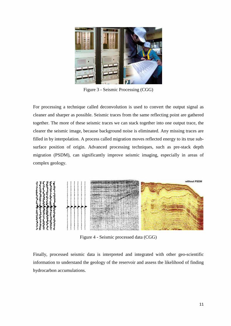
Figure 3 - Seismic Processing (CGG) ................................................................................. 11
Figure 4 - Seismic processed data (CGG) ........................................................................... 11
Figure 5 - Identification of seismic sequence boundaries (Selley R. , 1998) ...................... 13
Figure 6 - Seismic facies analysis: Reflection attributes (Bradley, 1985)........................... 14
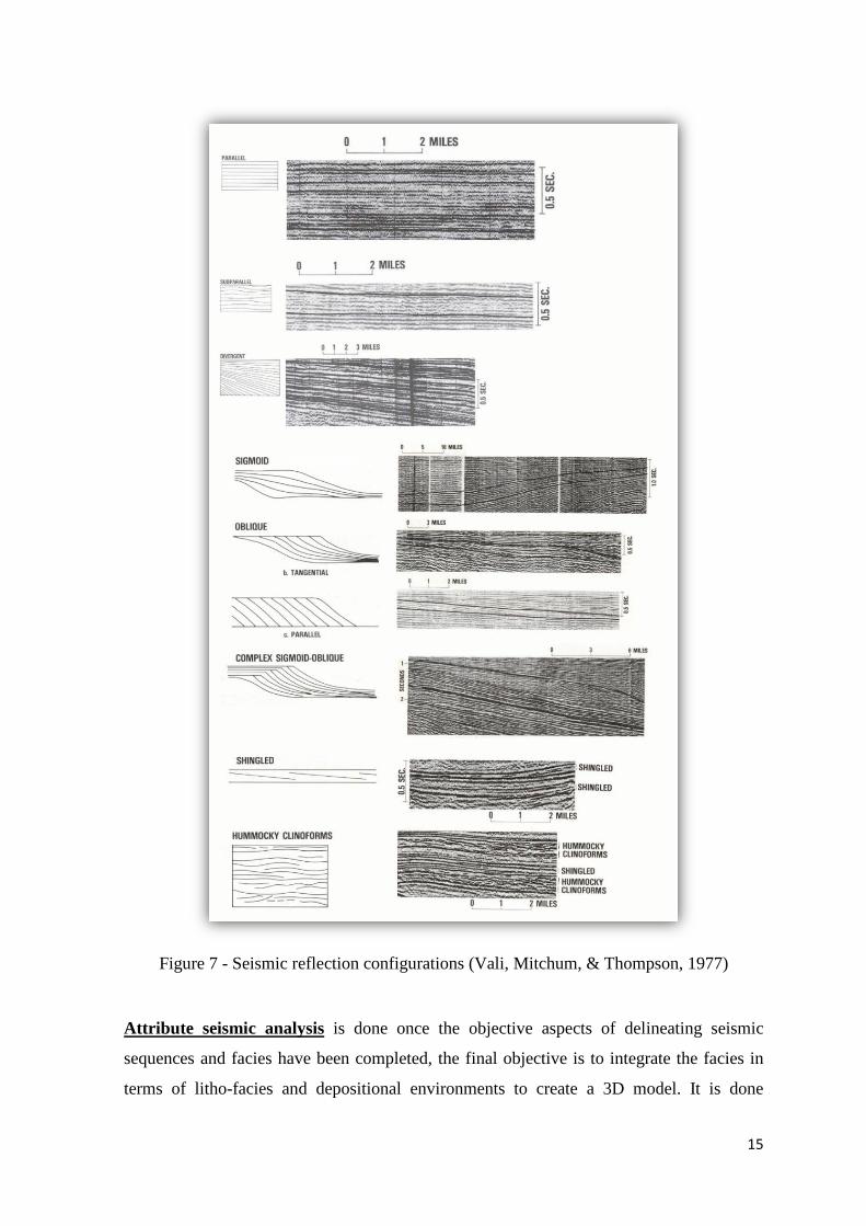
Figure 7 - Seismic reflection configurations (Vali, Mitchum, & Thompson, 1977) ........... 15
Figure 8 - Attribute seismic interpretation (Boggs, 2001)................................................... 16
Figure 9 - The borehole environment for well logging. (SPE, 2013) .................................. 18
Figure 10 - Gamma ray radiation of formation rocks (Darling, 2005) ................................ 19
Figure 11 - Reserves classification (Etherington J., 2005) .................................................. 25
Figure 12 - Regional tectonic location of Oriente-Maranon Basin (Xie Yinfu, 2010) ....... 32
Figure 13 - Oil structural corridors of Oriente Basin. (Modified from Baby, 2004)........... 33
Figure 14 – Paleogeography map of the Napo Formation, Oriente Basin .......................... 34
Figure 15 – Stratigraphy of the Oriente Basin (Dashwood M F, 1990) .............................. 35
Figure 16 – U and T sandstone of the Napo formation (J. Estupiñan R. M., 2010) ............ 38
Figure 17 - Hydrocarbon migration model Oriente Basin (Xie Yinfu, 2010) ..................... 39
Figure 18 - Methodology ..................................................................................................... 42
Figure 19 - Singue Field in Google Earth, location of wells Singue-1and Alama-1. .......... 43
Figure 20 - Well Singue-1 production ................................................................................. 48
Figure 21 - Singue-1 basic log interpretation. Lithology and well tops .............................. 60
Figure 22 - Alama-1 basic log interpretation. Lithology and well tops. ............................. 61
Figure 23 - Well correlation of Singue-1 and Alama-1. ...................................................... 63
Figure 24 - Clay volume interpretation ............................................................................... 65
Figure 25 - Saturation of fluids ........................................................................................... 66
Figure 26 - Net Pay intervals ............................................................................................... 68
Figure 27 - Seismic interpretation ....................................................................................... 71
Figure 28 - Well Tie ............................................................................................................ 72
Figure 29 - Horizon interpretation process .......................................................................... 74
Figure 30 – Horizon interpretation ...................................................................................... 74
Figure 31 - Fault interpreatation .......................................................................................... 75
xi
Figure 32 - Singue boundary ............................................................................................... 76
Figure 33 - Remaining Reserves Distribution ..................................................................... 78
LIST OF TABLES
Table 1 - Density of fluids (Myers, 2007) ........................................................................... 20
Table 2 – Napo formations sub-layers ................................................................................. 36
Table 3 - UTM and Geographic coordinates, Singue. Zone: 18S. Datum: WSG84 ........... 43
Table 4 - General Information of the wells. Singue-1 and Alama-1. .................................. 44
Table 5 - Biostratigraphy results of Singue-1 ...................................................................... 45
Table 6 - Singue 1 Core samples tests ................................................................................. 45
Table 7 - Volumetric information Napo U sanstone of Singue-1 ....................................... 46
Table 8 - Separation tests results at 100 F and 14.7 psi (U sanstone, Singue-1) ................. 47
Table 9 - Molecular composition of gas (Napo U, Singue-1) ............................................. 47
Table 10 - Well logs summary ............................................................................................ 49
Table 11 - Well tops from well log interpretation ............................................................... 62
Table 12a - SINGUE petrophysical results of the reservoir interval ................................... 69
Table 12b - SINGUE petrophysical results of the net pay interval ..................................... 69
Table 13a - ALAMA petrophysical results of the reservoir interval ................................... 69
Table 13b - ALAMA petrophysical results of the net pay interval ..................................... 69
Table 14 – Well tops ............................................................................................................ 72
Table 15 - STOIIP calculation results ................................................................................. 77
Table 16 - Reserves calculation results ............................................................................... 78
1
1. INTRODUCTION
1.1 INTRODUCTION
Singue is a small marginal oil field located in the Oriente Basin in Ecuador. Seismic
surveys and geophysical analysis were done on 1988 to define the exploitation of the field.
One exploratory well named Singue-1 was drilled on December 1990, at that time it was
part of the national oil company Petroecuador. During the drilling operation core samples
were analysed to define the rock properties of the reservoir. Additionally, analysis of the
fluid properties and initial production tests were done to make decisions about the
development of the field.
The exploratory well Singue-1 was successful. It reached an initial production of 500 bbl/
day and was kept in production with expectations of drilling more wells on the field in
order to increase the production of the national oil company at that time. During the
production stage one workover was developed due to a failure on the pump and one build
up well test was done to monitor the status of the wellbore. Shortly after, the priorities of
the national oil company shifted to more productive areas. The well was left in production
but no other wells were drilled. Singue-1 remained in production for 7 years. Afterwards
the well was closed due to highly increase in water cut and the field was finally abandoned
in 1997.
The objective of this dissertation is to analyse the present potential of the field. Available
data for this study includes geological information of the basin, seismic surveys of the area
and well logs of two wells in the field. The data will be used to calculate the volume of oil
in the reservoir. Historical production data will be used to define the situation at the end of
production time. Finally the estimation of further hydrocarbon available for commercial
use will be done. The effects of closing a well for more than 15 years were analysed in
order to estimate the production potential of the field. Analysis and discussion of results
will be used to make conclusions and suggest recommendations for further development of
the field.

2
1.2 OBJECTIVES
GENERAL OBJECTIVE 1.2.1
• Analyse the potential oil production of the field Singue of the Oriente Basin in
Ecuador.
SPECIFIC OBJECTIVES 1.2.2
• Analyse the geological information of the region and the available information
of the wells that are in the field.
• Analyse well logs to identify the lithology.
• Analyse well logs to calculate porosity, water saturation and net pay interval of
the sandstones.
• Run a simulation and interpretation of the seismic lines to establish the
accumulation of hydrocarbon.
• Calculate the original and remaining oil in place.
• Analyse the results of calculations and simulations to define the potential of
hydrocarbon in the field in order to suggest further work on it.
1.3 OUTLINE
The dissertation document in chapter one introduce an overview of the importance of oil in
Ecuador and a discussion about the desire of producing marginal fields to attend the local
energy demand and contribution for the country economical welfare. The second chapter
brings up the literature review which includes information about reservoir characterization
assessment and methods used to calculate oil in place and available oil reserves. The third
chapter introduces the geological information of the Oriente Basin, in which the field of
the present case of study is located.
Chapter four is focused on the methodology used to meet the objectives of the dissertation.
It includes an analysis of the provided data; the procedure used to perform well logging
analysis and seismic interpretation in specialized software in order to assess the location
and characterization of the reservoir defining some properties of the sandstones. At the end
of the methodology chapter the procedure to calculate remaining reserves is explained.

3
The results of the study are presented on chapter five with the corresponding discussion.
Finally, in chapter 6 are the conclusions and recommendations for further development in
the field. References and appendixes are attached on the last pages.
1.4 BACKGROUND
OVERVIEW OF IMPORTANCE OF PETROLEUM IN ECUADOR 1.4.1
All over the world petroleum is the mainly energy source. It is used in daily live for
transportation, domestic consumption and industrial applications. Therefore petroleum is a
strategic key factor that influences the economy of the nations and quality of life of the
people.
The prices of oil are established by the global consumption and by the offer of the
countries that produce this resource. OPEC is an organization in which are involved the
countries with the bigger hydrocarbon reserves. The aim of this organization is to protect
the member’s production and therefore their economy and development against the global
market in which are involved big transnational enterprises mainly based on developed
countries whose are the more energy consumers as well. OPEC plays an important role to
set the market price of oil.
Since petroleum was discovered it was used to produce energy making live more
comfortable for all their users. After the industrial revolution in 1970 the consumption
increased significantly in the countries where it took place. Developed countries were the
most consumers 40 years ago. Nowadays countries like China or India have become big
consumers because of their high population and their current industrial development. At
the end of the day the consumption is related with the population and technological level of
the country. Developed countries had reached a peak of consumption that has managed to
be steadily. In developing countries the consumption has been growing with expectations
of increment in the future. On the other side reserves of oil around the world have been
dropping through the years. For that reason the role of countries with the bigger reserves is
very important.

4
Investments with the aim of discovering new energy sources and technology development
to improve current production systems are done everywhere. Even if there are new energy
sources such as hydroelectricity, nuclear and sustainable; fossil based resources that
includes coal, petroleum and natural gas are still the most used. Petroleum is the most
important resource and natural gas has a greater foresight. The aim is to ensure energy
supplying to meet the growing global energy consumption.
In this context, one important problem is that most of the producer countries still are in
developing conditions and they do not have the technology, on the other hand consumer
countries that have the technology through the time are getting out of the resource. This
has made producer developing countries to export crude oil for cash. There are some
countries that sell crude oil and import final products like diesel, gasoline, LPG or
lubricants. Then could be understood the close relationship and dependence between
producers, consumers and their economies.
The last 5 years the price of oil have been as higher an ever, above 100 US dollars per
barrel. This has promoted the investment on the oil industry all around the world and
therefore and increasing wealthy of the countries that have the resource. Compared with
the beginning of the industry the situation has improved. Nowadays, State-owned national
oil companies control 90% of the world's conventional petroleum resources. As a result in
some countries such as Ecuador, private companies have increasingly focused on projects
located in marginal areas that are often inhabited by indigenous, tribal and minority
groups; in other words they are left to work on more costly, dangerous and risky areas.
(Wasserstrom, 2013). This fact is notably fairer for the country than in previous times.
The amazon region of Ecuador is located in the Oriente Basin. The first oil well was
discovered in 1967. Since then the country has changed to oil production as the main
economic income. Two types of crude oil have been discovered in the country: the first
called “Oriente” that has an API gravity of 26, and the second which is heavier is called
“Napo” with an API gravity of 19. Ecuador was member of OPEC from 1973 to 1993 and
then, re-joined in 2007. There are some refineries to supply the local consumption; the rest
of the crude is exported representing an important weight in the gross domestic product
(GDP) of the nation.
5
At the present, the national oil company called Petroecuador is the main operator of the
production fields; however few fields are in charge of international companies under
service contracts. The aim of the government is to let private companies to develop less
cost effective or high risk fields. In this group are the heavy oil fields, some mature and the
marginal fields. Heavy oil fields are the ones with petroleum with API gravity below 15.
Mature fields are those that have been producing for more than 30 years showing a
significantly drop on the production rate; those represent a challenge to develop middle
and long term strategies and may be an interesting opportunity to implement new
technologies to enhance the production. In addition there are the marginal fields which
have low economic or operational priority, and represent less than 1% of total national
production (Petroecuador, 2010). Marginal fields are very risky because of their small size
and based on previous experiences, they can easily disappear if there are problems with the
speed of production. Once those are put into production, oil can easily be flooded, because
of the small oil column compared to the very strong formation water.
Even though, the marginal fields are not priority of the national government those are
important for private companies that want to invest, summing up that any increasing in
production will benefit the government to maintain the current daily production quota
established by the OPEC.
The government of Ecuador since the year 2007 is driving a campaign to optimize the oil
production in all the country with appropriate environmentally and social caution. In this
program the less cost effective and risky fields have been put out to tender for development
to private companies seeking investment. The analysis of one of the marginal fields named
Singue that is considered one of the marginal fields of Ecuador is the purpose of this
dissertation. The company, Dygoil & Gente Consortium (DGC), had been in charge of the
operation of the field since 2012. Dygoil have provided the information to develop this
project. In Appendix 1 is attached the authorization letter that states the use of the provided
documentation for this project with strictly academic purposes of the author.
MARGINAL FIELDS 1.4.2
The article two of the Ecuadorean Law of Hydrocarbons stands that "marginal fields are
those of low operational or economic priority, so considered because found far from
6
Petroecuador infrastructure, to contain low gravity crude oil or heavy oil, or because
require techniques of excessively costly recovery. These fields may not represent more than
1% of the national production and will be subject to the international conservation
reserves fee." (PGE, 2013).
1.5 LIMITATIONS OF THE PROJECT
In the present project the author found certain difficulties that might affect to some extend the
results, among them are:
• From the case of study, because Singue is a non-developed field there are only two wells in the
area. It is recommended to have at least three wells to make a reservoir model. Even though the
model was not finished, the calculations that correspond to the first stage of oil exploration
were developed successfully to get results and meet the objectives of this project.
• From the available data of the area, seismic lines are 2D and are not so close, for that reason
some assumptions were done to get the boundary of the reservoir. Additionally, some available
seismic lines that have different resolution were not taken in consideration for the
interpretation.
• The method used in the calculation of reserves is the volumetric method.
• The use of Petrel and Interactive Petrophysics in short time has been a big challenge. Some
lack of experience in the programs might influence in the decision of running some
calculations in the programs with default parameters, nevertheless results have been
satisfactory obtained.

7
2. LITERATURE REVIEW
2.1 RESERVOIR EXPLORATION
A reservoir is a rock with the capability of hydrocarbon accumulation. The rock to act as a
reservoir must have pores to contain the oil or gas and the pores must be connected to
allow the movement of fluids, in other words the essential characteristics are the porosity
and permeability. Most of the oil and gas reserves have been founded in sandstones and
carbonates.
The exploration is the first stage in order to find hydrocarbon. It consists in the geological,
geophysical and petro-physical study of the earth rock layers of the possible oil reservoir.
Exploration stage concludes with the drilling of an appraisal well that will demonstrate the
existence of oil.
Geological knowledge is used to understand the development of the hydrocarbon basin in
which the reservoir rock is present. The reservoir sedimentary rock must be porous and
with a structure capable of trapping the hydrocarbon. The analysis of the geological time of
the region is used to define the organic depositional environment and sedimentary
depositional sequence of the basin. Superficial rock samples, electric log interpretations
and down-hole samples are acquired during the drilling and are used to understand the
geology of the region.
Geophysical studies are used to define the lithology, structure of the reservoir in order to
determine the probable oil accumulation zones known as facies. After having enough
information of the region, geophysical seismic prospective is done. Specialised tools
generate explosive waves that are reflected and recorded by geophones; a lineal
radiography of the subsurface is created in specialized technical software. Interpretation of
the results must define the accurate region where hydrocarbon is stored.
As was mentioned, the only way to determine the existence of oil is drilling an appraisal
well. Therefore the next stage is to drill a well in the most probable analysed zone. During
the drilling, more information of the reservoir is obtained by samples and logs that are
interpreted to define more accurate properties of the reservoir. Petrophysical analysis of the

8
well logs will determine the rock properties such as porosity, permeability and fluid
saturation. Pressure-volume-temperature (PVT) analysis of the fluid is done to determine
the type of hydrocarbon available; properties such as API gravity, viscosity, density,
bubble point are found.
The results of the appraisal well will determine investment on the field. When the well is
on production, analysis of the driven mechanism of the reservoir and composition of the
fluid could be done. As long as more wells are drilled more information could be collected
and better representation of the reservoir could be done to assess the calculation of reserves
and the effective way of recovering as much petroleum as economically possible. (Weber
& Van Genus, 1990)
A reservoir characterization is a model of the reservoir that includes all the parameters that
will define the ability of storage and production of the hydrocarbons. To characterize a
reservoir two models could be created:
• Geological static model: Created by geologists and geophysicists to provide a static
description of the reservoir before production.
• Reservoir dynamic model: Created by reservoir engineers to simulate the flow of fluids
within the reservoir during the production lifetime.
The geological model can be used to predict the distribution of porosity, permeability and
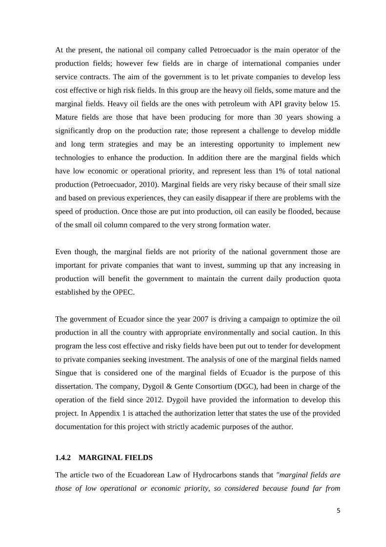
fluids in the field. Based on the geometric complexity the reservoir model could be layer
cake, jigsaw puzzle or labyrinthine type shown in (Figure 1). Whatever it is, it can be
modelled deterministically using geology or probabilistically using statics. For any
appraisal used, the objective is to produce a three dimensional grid of the field with a
specific value of porosity, permeability and petroleum saturation within each cell of the
grid. Once the model is created the hydrocarbon reserves could be calculated and the
production method could be simulated in a computer. (Tarek H, 2004)
9
Figure 1 - Reservoir geological modelling types (Weber & Van Genus, 1990)
The present project is focused on the geophysical and petrophysical interpretation of the
seismic lines well logs in order to determine the potential of oil available in the reservoir.
2.2 GEOPHYSICAL EXPLORATION
Geophysical exploration is the applied branch of geophysics that uses surface methods to
measure the physical properties of the subsurface Earth, along with the anomalies in these
properties, in order to detect the presence and position of minerals, hydrocarbons,
geothermal reservoirs, groundwater reservoirs, and other geological structures.
Geophysical exploration includes three types: the magnetic method, the gravity method
and the seismic surveying. The first two are used only in pre-drilling phase, but seismic is
used in both exploration and development phases. Seismic is the most important method
because integrates the knowledge of geologists and geophysics with physic, mathematics
and computing engineering to create a virtual model of the reservoir.
The integration of seismic surveying with geophysical logs is referred as Borehole
Geophysics and is used to generate a four dimensions model capable to give an efficient
image of the reservoir with properties prior to the identification of hydrocarbons. In later
stage it is used to the development and expansion of the field. (Darling, 2005)
10
SEISMIC SURVEYING 2.2.1
The principle of seismic is to create reflecting waves to estimate the properties of the
Earth. Seismic surveying consist in three stages: data acquisition, data processing and
interpretation.
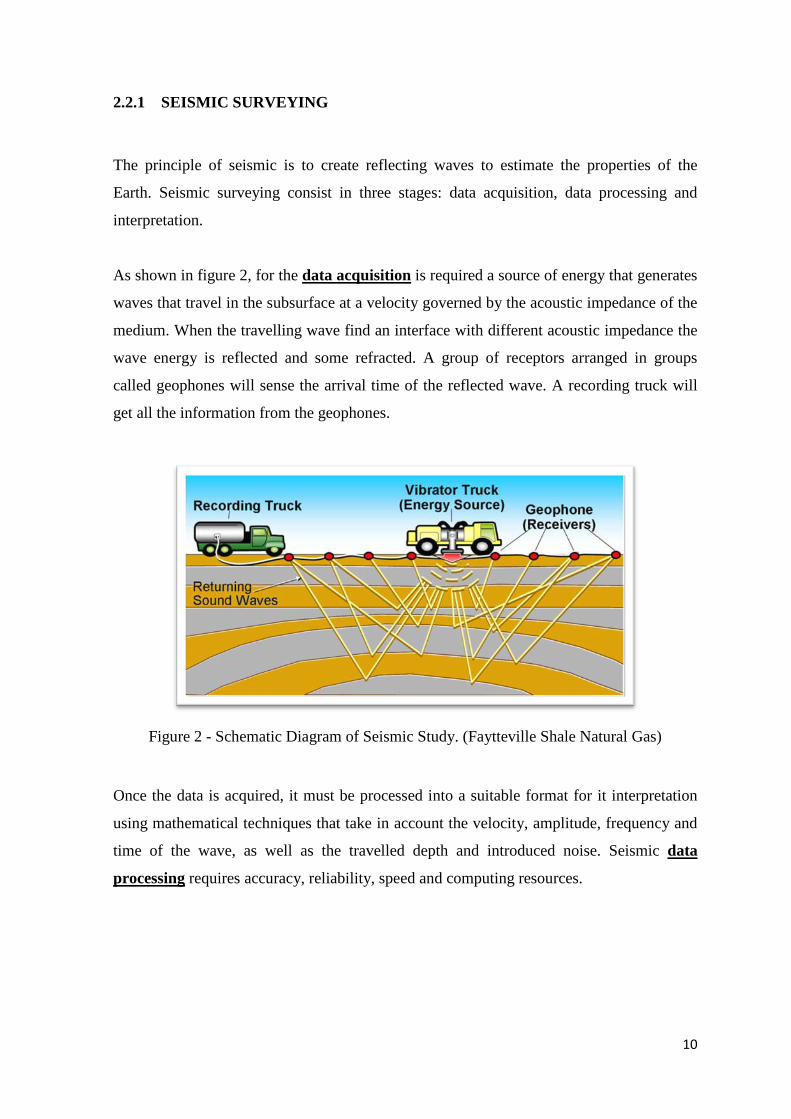
As shown in figure 2, for the data acquisition is required a source of energy that generates
waves that travel in the subsurface at a velocity governed by the acoustic impedance of the
medium. When the travelling wave find an interface with different acoustic impedance the
wave energy is reflected and some refracted. A group of receptors arranged in groups
called geophones will sense the arrival time of the reflected wave. A recording truck will
get all the information from the geophones.
Figure 2 - Schematic Diagram of Seismic Study. (Faytteville Shale Natural Gas)
Once the data is acquired, it must be processed into a suitable format for it interpretation
using mathematical techniques that take in account the velocity, amplitude, frequency and
time of the wave, as well as the travelled depth and introduced noise. Seismic data
processing requires accuracy, reliability, speed and computing resources.
11
Figure 3 - Seismic Processing (CGG)
For processing a technique called deconvolution is used to convert the output signal as
cleaner and sharper as possible. Seismic traces from the same reflecting point are gathered
together. The more of these seismic traces we can stack together into one output trace, the
clearer the seismic image, because background noise is eliminated. Any missing traces are
filled in by interpolation. A process called migration moves reflected energy to its true sub-
surface position of origin. Advanced processing techniques, such as pre-stack depth
migration (PSDM), can significantly improve seismic imaging, especially in areas of
complex geology.
Figure 4 - Seismic processed data (CGG)
Finally, processed seismic data is interpreted and integrated with other geo-scientific
information to understand the geology of the reservoir and assess the likelihood of finding
hydrocarbon accumulations.

12
SEISMIC INTERPRETATION 2.2.2
The interpretation of seismic is a very important part of the petroleum exploration because
it could be used to regional mapping, prospect mapping, reservoir delineation, seismic
modelling, hydrocarbon detection and monitoring of production. (Selley, 1998) Seismic
stratigraphic analysis is carried out in a logical series of steps: the seismic sequence, facies
and attributes analysis.
Seismic sequence analysis is based on the identification of stratigraphic units composed of
a relatively conformable succession of genetically related strata called depositional
sequence. The upper and lower boundaries of depositional sequences are unconformities or
correlative conformities. Those are recognized on seismic data by identifying reflections
caused by lateral terminations (Figure 5). In practice it separates out time-depositional
units based on detecting unconformities or changes in seismic patterns.
(Selley R. , 1998) Three main types of reflection discordance are:
• Erosional truncation: is the termination of strata against an overlying erosional surface.
• Apparent truncation: is the termination of relatively low-angle seismic reflections
beneath a dipping seismic surface, where that surface represents marine condensation.
• Lapout: is the lateral termination of a reflection at its depositional limit.
o Onlap: is recognized on seismic data by the termination of low-angle reflections
against a steeper seismic surface. Two types of onlap are recognized: marine
onlap and coastal onlap.
o Downlap: is a baselap in which an initially inclined stratum terminates downdip
against an initially horizontal or inclined surface. The surface of downlap
represents a marine condensed unit in most cases.
o Toplap: is the termination of inclined reflections against an overlying lower
angle surface, where this is believed to represent the proximal depositional
limit.

13
Figure 5 - Identification of seismic sequence boundaries (Selley R. , 1998)
The steps for depositional sequence analysis are summarized below:
1. Determine the vertical and horizontal scale of the section.
2. Define if it is migrated section and if it is marine or land data.
3. Identify multiples such as water-bottom multiples, peg-leg multiples, etc. and mark
them in light blue.
4. Identify and mark reflection terminations or unconformities (onlap, downlap, and
truncation) with arrowheads in red.
5. Identify seismic surfaces on the basis of reflection terminations. Assign a specific
colour to individual seismic surface based on its type or age.
6. Identify sequence boundaries. Sequence boundaries are commonly marked by
truncation or onlap, whereas maximum-flooding surfaces are commonly marked by
downlap.
7. Carry out a similar exercise on other intersected seismic lines and tie the seismic
surfaces and interpretation around the data set.
8. Map sequence units on the basis of thickness, geometry, orientation, or other
features to see how each sequence relates to neighbouring sequences.
9. Identify seismic facies for each sequence.
10. Interpretation of depositional environments and lithological facies.
Seismic facies analysis is the description and geological interpretation within sequences of
smaller reflection units that may be the seismic response between boundaries. It analyses

14
the configuration, continuity, amplitude, phase, frequency and interval velocity. These
parameters indicate the lithology and sedimentary environment of the facies. (Figure 6)
Figure 6 - Seismic facies analysis: Reflection attributes (Bradley, 1985)
Parallelism of reflections to cross bedding or to physical surfaces that separates older from
younger sediments are defined as reflection configurations, and are helpful to identify
stratification patterns, depositional processes, erosion and paleo-topography.
Some reflection patterns are (Figure 7):
• Parallel and subparallel
• Divergent
• Prograding: Sigmoid, oblique, complex sigmoid-oblique, shingled or hummocky.
• Chaotic
• Reflection free
15
Figure 7 - Seismic reflection configurations (Vali, Mitchum, & Thompson, 1977)
Attribute seismic analysis is done once the objective aspects of delineating seismic
sequences and facies have been completed, the final objective is to integrate the facies in
terms of litho-facies and depositional environments to create a 3D model. It is done

16
examining the lateral variation of individual reflection events to locate where stratigraphic
changes occur and identify their nature; the primary tool for this is synthetic seismograms
and seismic logs.
Figure 8 - Attribute seismic interpretation (Boggs, 2001)
2.3 WELL LOGGING
Logs are run after drilling into the open hole or completed well to measure petrophysical
properties of the formations and to assess in the geophysical analysis of the reservoir. The
well logs measure many parameters of the rock such as formation resistivity, sonic
velocity, density and radioactivity of the elements. Interpretation of the results is used to
determine the lithology, porosity of the formation, type of fluid and saturation. Logs could
be interpreted manually but, nowadays specialized computer programs process the logs to
give accurate and faster results.
WELL LOG TYPES 2.3.1
Below are described some of the types of logs commonly used in the petroleum
exploration industry.
a. Spontaneous Pontential (SP)
SP is a log that measures the natural difference in electrical potential between an electrode
in the borehole and a fixed reference electrode on the surface. It can be used in open holes
filled with conductive mud. The SP response is dependent on the difference in salinity

17
between drilling mud and the formation water. SP is used to identify permeable zones,
therefore the lithology of the well; and also could be used to calculate the formation water
resistance. Porous sandstones with high permeability tend to generate more electricity than
impermeable shales. Thus, SP logs are often used to differentiate sandstones from shales.
(SPE, 2013)
b. Resistivity logs
Resistivity logs determine the type of fluid that is present in reservoir rocks by measuring
how effective are these rocks to conducting electricity. Because fresh water and oil are
poor conductors of electricity they have high resistivity. By contrast, most formation
waters are salty enough that they conduct electricity with ease. Thus, formation waters
generally have low resistivity.
The resistivity (R) of a substance is the electrical resistance measured between opposite
faces of a unit cube of the substance at a specified temperature:
Where,
R = resistivity in ohm-m,
r = resistance in ohm,
A = area in m2,
L = length in m.
Conductivity (σ) is the reciprocal of resistivity and is expressed in milliSiemens per meter
[mS/m]:
Formation resistivity is measured by passing a known current through the formation and
measuring the electrical potential or by inducing a current distribution in the formation and
measuring its magnitude. It is usually in the range of 0.2-1000 [ohm-m]; higher resistivity
values are uncommon in most permeable formations but are observed in low porosity
formations such as evaporites. The resistivity of the borehole is commonly much less than
the formations of interest that generally consists of rock layers with widely varying
resistivity. (Figure 9)

18
Figure 9 - The borehole environment for well logging. (SPE, 2013)
The main objectives of resistivity logs are the determination of Rt and Rxo and, for the
newer imaging devices, the mapping of resistivity profiles into and around the borehole.
There are many different types of resistivity logs, which differ in how far into the rocks
they measure the resistivity (San Joaquin Valley Geology):
• The deep laterolog device (LLd)
• The deep induction device (ILd)
• The shallow laterolog (LLs)
• The medium induction (ILm)
• The microresistivity device
• The spherically focused log (SFL)
c. Gamma Ray (GR)
GR logs measure radioactivity to determine the types of rocks in the well. Natural
occurring radioactive materials (NORM) include the elements uranium, thorium,
potassium, radium and radon. Logging tools have been developed to read the gamma rays
emitted by these elements and interpret lithology from the information collected. It is
particularly used to distinguish sands from shales.

19
(Russell, 1944) In figure 10, the distributions of radiation levels observed by Russell are
plotted for numerous rock types. Evaporites (NaCl salt, anhydrites) and coals typically
have low levels. In other rocks, the general trend toward higher radioactivity with
increased shale content is apparent. At the high radioactivity extreme are organic-rich
shales and potash (KCl).
Figure 10 - Gamma ray radiation of formation rocks (Darling, 2005)
d. Neutron logs
Neutron logs or compensated neutron logs (CNL) determine porosity by assuming that the
reservoir pore spaces are filled with either water or oil; and then measure the amount of
hydrogen atoms (neutrons) in the pores. If the lithology is known, the neutron log can be
used to calculate porosity. Generally, the neutron and density logs are run together.
The level of radiation reaching the detector is inversely related to the hydrogen content as
shown below:
• High Porosity = High hydrogen content = Low GR
• Low Porosity = Low hydrogen content = High GR
Gas has a very marked effect on both density and neutron logs. If it is assumed that the
formation fluid is water and the invasion zone is shallow, then gas will result in a lower

20
bulk density and lower apparent neutron porosity. In limestone and dolomites, the lithology
of a gas zone may show up as sandstone. The gas contact can sometimes be easily
identifiable in carbonates from the raw logs, as they are frequently plotted on a limestone
scale. The gas will cause the density log to be abnormally low, at the same time the
neutron porosity will read too low. (Myers, 2007)
e. Density logs
Density logs or formation density compensated logs (FDC), determine porosity by
measuring the density of the rock. It belongs to the group of active nuclear tools, which
contains a radioactive source and two detectors. Tools rely on gamma-gamma scattering or
on photoelectric (PE) absorption.
The bulk density (𝜌b), from the density log is the sum of the density of the fluid (𝜌f) times
it relative volume (∅) plus the density of the matrix (𝜌ma) times it relative volume (1 − ∅),
or:
There is some variation in grain density. Dolomites can vary from 2.83 to 2.87. Generally,
the density tool will read mostly the flushed zone. Recommended density filtrate values are
1.0, 1.1 and 0.90 gm/cc for freshwater, saturated salt water, and oil based muds,
respectively. A list of reference densities for common materials is shown in table 1.
Table 1 - Density of fluids (Myers, 2007)
f. Sonic logs
Sonic logs or borehole compensated (BHC) logs are used to determination of porosity,
identification of gas intervals and cement evaluation. In general, those measure how fast
21
sound waves travel through rocks in the well. Sound waves travel faster through high
density shales than through low density sandstones.
g. Nuclear magnetic resonance logs (NMR)
NMR logs measure the magnetic response of fluids present in the pore spaces of the
reservoir rock and are used to determine porosity and permeability, as well as the types of
fluids present in the pore spaces.
h. Dip-meter logs
Dip-meter logs determine the orientations of sandstone and shale beds in the well, as well
as the orientations of faults and fractures. Modern dip meters could make a detailed image
of the rocks on all sides of the well hole. Borehole scanners do this with sonic waves, FMS
(formation micro scanner) and FMI (formation micro-imager) logs do this by measuring
the resistivity. These type of 3D logs are known as image logs since they provide a 360°
image of the borehole that can show bedding features, faults and fractures, and even
sedimentary structures.
FORMATION EVALUATION 2.3.2
The formation evaluation is the complete process of analysing well logs to get the
petrophysical characteristics of the formation. Required parameters for volume calculations
are: Volume of shale, porosity, water saturation and thickness of the reservoir.
The shale volume estimation (Vsh) is calculated using values of the gamma ray (GR),
spontaneous potential (SP), neutron (PHIN) and density (PHID) porosity logs.
𝑉𝑠ℎ𝑔 = 𝐺𝑅 − 𝐺𝑅𝑐𝑙𝑒𝑎𝑛
𝐺𝑅𝑠ℎ𝑎𝑙𝑒 − 𝐺𝑅𝑐𝑙𝑒𝑎𝑛
𝑉𝑠ℎ𝑠 = 𝑆𝑃− 𝑆𝑃𝑐𝑙𝑒𝑎𝑛𝑆𝑃𝑠ℎ𝑎𝑙𝑒−𝑆𝑃𝑐𝑙𝑒𝑎𝑛
𝑉𝑠ℎℎ𝑥 = 𝑃𝐻𝐼𝑁− 𝑃𝐻𝐼𝐷𝑃𝐻𝐼𝑁𝑠ℎ𝑎𝑙𝑒−𝑃𝐻𝐼𝐷𝑠ℎ𝑎𝑙𝑒
22
GR, SP, PHIN and PHID are the picked log values, while clean and shale indicates values
picked in the clean and shale base lines, respectively.
Porosity from logs is considered total porosity (PHIt), which includes the bound water in
the shale; to obtain effective porosity (PHIe) it must be corrected for shale volume. When
both the neutron and density porosity curves are available, as in this case, the best method
for correcting porosity is the complex lithology Density/Neutron crossplot. First, porosity
is corrected for shale volume by PHIxc = PHID – (Vsh × PHIshale), where x will be n for
neutron or d for density porosity. Effective porosity is then calculated as:
𝑃𝐻𝐼𝑒 = 𝑃𝐻𝐼𝑛𝑐 − 𝑃𝐻𝐼𝑑𝑐2
To calculate water saturation, most methods require a water resistivity (Rw) value. In this
case, an obvious clean water zone is present in two of the wells in the area and the water
resistivity was calculated from the porosity and resistivity in this zone, using the Ro
method, given by the following equation:
𝑅𝑊@𝑓𝑜𝑟𝑚𝑎𝑡𝑖𝑜𝑛 𝑡𝑒𝑚𝑝𝑒𝑟𝑎𝑡𝑢𝑟𝑒 = 𝑃𝐻𝐼𝑤𝑡𝑟𝑚 𝑅𝑜
𝑎
RW@FT is the water resistivity at formation temperature, PHIwtr and Ro are the total
porosity and deep resistivity values in the water zone, a is the tortuosity factor and m is the
cementation exponent.
2.4 SUBSURFACE GEOLOGY
Successful petroleum exploration involves the integration of geophysical seismic surveys
and wire line logs with geological data and concepts. When information of more than one
well is available, stratigraphic correlations could be done and summed up to the logs are
used to determine the facies and depositional environment of the reservoir. Vertical cross
sections are created to understand the geological data from small scale sections up to
regional sections.
WELL CORRELATION 2.4.1
The first stage for create a cross section is based on well correlation. When a well is drilled
and logged, a correlation of the geological data gathered from well cuttings with well logs

23
is generated. Firstly, the formation tops are picked at a specific depth by the geologist,
palaeontologist and geophysicist. Then correlation of the tops is correlated with adjacent
wells based on the geophysical logs. The gamma, sonic and resistivity curves all the most
used.
Some useful marks are coal beds and limestone, which are thin but show exaggerate kicks
on resistivity and porosity logs. Examination of the appropriate seismic data is necessary
because sometimes significant intervals may be missing caused by depositional thinning,
erosion or faulting. Repetition of sections caused by reverse faulting in sections subjected
to compressional tectonics also may be noted.
GEOLOGICAL CROSS SECTIONS 2.4.2
After the formation tops have been picked and the wells correlated, a cross section may be
created with datum which could be sea level, fluid contact or a particular geological
horizon. The procedure is simple for vertical wells, but more complex for deviated or
horizontal ones in which the true vertical depth may be used.
Cross sections of fields are based on well control. Seismic and well data is used for
regional studies. A development of a single cross section is a series of drawings using a
sequence of different data horizons that nowadays also is done by specific computer
programs.
SUBSURFACE MAPS 2.4.3
Many types of geological maps are used for oil exploration. As much information is
available the accuracy of the interpretation will increase. Some of these geological maps
are:
• The structure contour maps indicate the morphology of the basin and the traps based on
seismic data and well logs. These maps are useful for reserves calculation.
• Isopach maps record the thickness of formations based on seismic and well logs.
• Isochore maps is a particular type of isopach that indicates the thickness of the interval
between the oil-water contact and the cap rock of the trap.
24
• The net pay map contours the ratio of gross pay to net pay within the reservoir.
• Sand-shale ratio maps indicate the source of sandstones and therefore possible
reservoir areas.
• Paleogeographic maps are based on seismic and well logs of a section in which the
depositional environment has been interpreted. Those are used to predict the quality of
source rock and reservoirs.
The combination of the maps is used to delineate plays and prospects where hydrocarbon
could be found.
CORING ANALYSIS 2.4.4
During the exploration phase, coring samples are analysed in order to get more information
of the reservoir and calibrate the petrophysical model with data not obtained by the well
logs.
The information obtained from basic coring analysis is:
• Homogeneity of the reservoir
• Type of cementation and distribution of porosity and permeability
• Types of minerals in the reservoir
• Presence of fractures and their orientation
• Dip features that may influence logging tools response.
2.5 RESERVES ESTIMATION
Oil reserves are the amount of technically and economically recoverable oil. Reserves may
be calculated for a well, reservoir, field, or a nation. Estimation of reserves can be done
before a field have been drilled with approximate data that may give an indication of the
economic viability of the projects. As the field is being developed and produced, accurate
reserves could be known. Several methods are used to estimate reserves depending on the
availability of data.
25
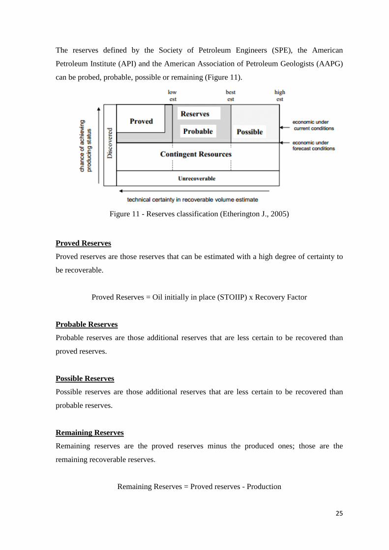
The reserves defined by the Society of Petroleum Engineers (SPE), the American
Petroleum Institute (API) and the American Association of Petroleum Geologists (AAPG)
can be probed, probable, possible or remaining (Figure 11).
Figure 11 - Reserves classification (Etherington J., 2005)
Proved Reserves
Proved reserves are those reserves that can be estimated with a high degree of certainty to
be recoverable.
Proved Reserves = Oil initially in place (STOIIP) x Recovery Factor
Probable Reserves
Probable reserves are those additional reserves that are less certain to be recovered than
proved reserves.
Possible Reserves
Possible reserves are those additional reserves that are less certain to be recovered than
probable reserves.
Remaining Reserves
Remaining reserves are the proved reserves minus the produced ones; those are the
remaining recoverable reserves.
Remaining Reserves = Proved reserves - Production

26
The volumetric method is the most common methodology used for estimation of reserves.
The precision of porosity, water saturation and volume of the reservoir will determine the
hydrocarbon calculated volume.
PRELIMINARY VOLUMETRIC CALCULATION 2.5.1
A rough estimation of reserves can be calculated assuming that the trap is full of fluid
using the following equation:
Recoverable oil reserves (bbl) = 𝑉𝑏 x RF
Where,
Vb = Bulk Volume
F = Recoverable oil (bbl/acre-ft)
The bulk volume is calculated from the area and closure estimated from seismic data with
the following equation:
𝑉𝑏 = h �𝑎02
+ 𝑎1 + 𝑎2+. . +𝑎𝑛−1 + 𝑎𝑛2�
Where,
Vb = Volume
h = Contour interval
ao= area enclosed by oil-water contact
a1= area enclosed by first contour
an= area enclosed by nth contour
The recoverable oil is difficult to assess unless local information is available from adjacent
fields. It may be calculated with an estimate of the average porosity of the reservoir. Since
only a certain amount of hydrocarbon could be recovered of the total oil in place and is
called recovery factor. It will be affected by the type of rock, the reservoir production
driven mechanism and the fluid properties. The recovery factor used for oil is about 10-
20% for carbonate reservoirs and 30% for sandstones.

27
POST-DISCOVERY RESERVES CALCULATIONS 2.5.2
Original oil in place (OOIP) or Oil initially in place (OIIP) is the total volume of
hydrocarbon content of an oil reservoir before beginning of the production and is
calculated with the following equation for stock tank barrel units:
STOIIP (STB) = 7758 × A×th × Φ ×(1−Sw) Bo
…… Eq. 1
Where,
V = Volume of the reservoir (A x h)
A = Area of the reservoir (acres)
th = Thickness of pay zone (ft)from logs
7758 = Conversion factor from acre-feet to barrels
Φ = Average rock porosity (decimal) from logs
Sw = Average water saturation (decimal) from logs
Bo = Formation volume factor for oil at initial conditions
When oil is produced, the high reservoir temperature and pressure decreases to surface
conditions and gas bubbles out of the oil. As the gas bubbles out of the oil, the volume of
the oil decreases. Stabilized oil under surface conditions (60o F, 14.7 psi) is called stock
tank oil; it could be expressed as stock tank barrel (STB).
Since the reserves are the volume that can be recoverable, when a well is drilled accurate
reservoir data become available and an efficient calculation of reserves could be done with
the appropriate recovery factor:
Recorvable oil (bbl) = STOIIP × RF …….Eq. 2
Where,
STOOIP = Initial oil in place (STB)
RF = Estimated recovery factor

28
Oil formation volume factor (Bo) converts a stock tank barrel of oil to its volume at
reservoir pressure and temperature. It depends on oil composition, but it is approximated
by calculating the gas-oil ratio (GOR) and oil density (API gravity). It usually varies from
1.0 for heavy crudes with low GOR up to 1.7 for volatile oils and high GOR.
GOR (in the reservoir) = 𝑄𝑔𝑄𝑜
= 𝜇𝑜𝐾𝑔𝜇𝑔𝐾𝑜
Where,
Q = Flow rate at reservoir pressure and temperature
g = gas
o = oil
µ = Viscosity at reservoir pressure and temperature
K = Effective permeability
An accurate measurement of Bo and GOR are done in laboratory with fluid samples. This
procedure is referred as pressure-volume-temperature (PVT) analysis.
Petro-physical analysis based on the well logs is used to assess the properties of the
reservoir rock. In addition, during the drilling of each well some rock core samples of the
reservoir are analysed in the laboratory to assess the initial information of porosity,
permeability, water saturation and other necessary reservoir properties acquired with the
logs.
As the field is produced several changes take place in the reservoir such as pressure drops
and decreases in flow rates. The GOR also changes depending on the production driven
mechanism. The changes are analysed with a material balance equation (MBE) that is
based on the law of mass conservation.
MBE relates volumes of fluid in the reservoir at initial pressure with produced and
remaining volumes at any stage of the production life. Dynamic modelling of the reservoir
is based on the material balance and more complex relations.

29
2.6 SOFTWARE
PETREL 2.6.1
Hydrocarbon exploration integrates geophysical exploration, well logging and geology
concepts. Technological development makes exploration work more efficient and less time
consuming due to specialized computing tools developed for this purpose. Several software
packages for geologic modelling of reservoirs can display, edit, digitise and automatically
calculate the parameters required by engineers, geologists and surveyors for exploration
phase as well as any other stage of hydrocarbon production.
(Schlumberger, 2014) Petrel is a Schlumberger owned Windows PC software application
intended to aggregate oil reservoir data from multiple sources. It allows the user: to
interpret seismic data, perform well correlation, build reservoir models suitable for
simulation, submit and visualize simulation results, calculate volumes, produce maps and
design development strategies to maximize reservoir exploitation. It integrates in a single
application the "seismic-to-simulation" workflow.
A probabilistic analysis of the volumetric equations described previously is done with the
required distributions of uncertainty for each parameter which, apart from the gross rock
volume, reflect the average value of that parameter over the area or volume for which oil in
place is being calculated. It takes in consideration not the hole reservoir but to be more
precise, the average net pay over the area of the reservoir, the average porosity over the
bulk volume, and the average oil saturation over the net pore volume. These computations
are often dealt with through the application of 3D geological models. Since the equation
requires the use of averages for reservoir properties as input, it is the uncertainty in the
reservoir average that must be the basis for a probabilistic analysis. (Murtha J., 2009)
Reservoir simulators in Petrel are classified according the type of fluid:
• Gas reservoir simulator: Single phase or two phase reservoirs.
• Black oil reservoir simulator: Gas, oil and water present in the reservoir.
• Compositional reservoir simulator: Condensate and volatile oil reservoirs.
After the type of model has been selected, the reservoir is divided into blocks; each block
is assigned with the rock properties (porosity and permeability), geometrical data (cell

30
dimensions and thickness) and the well data (phase saturation, relative permeability,
capillary pressure, PVT). If field data exist therefore an accurate performance predictions
can be done, if data is not available simulators may compare qualitatively the results of
different ways of operating the reservoir. Accuracy of results could be done by history
matching techniques.
The following steps are required to build a 3D geological model of a petroleum reservoir:
1) Data Import
2) Input Data Editing
3) Well Correlation
4) Fault Modeling
5) Pillar Gridding
6) Vertical Layering
7) Geometrical Property Modeling
8) Upscaling in the Vertical Direction-Well Logs Upscaling
9) Facies Modeling
10) Petrophysical Modeling
11) Defining Fluid Contacts
12) Volume calculations
INTERACTIVE PETROPHYSICS (IP) 2.6.2
(Senergy Software Ltd., 2011) IP is a fast, flexible and robust software package that is used
by petrophysicists, geologists and reservoir engineers to perform well logging analysis
offering control and flexibility through a friendly and intuitive interface. IP offers some
interpretation modules such as: Basic log analysis, Mineral solver, Monte Carlo simulation,
Saturation Height modelling, Statistical prediction modules, Rock physics interpretation,
Pore pressure prediction, Formation test, Date-Time well, Real-Time data and Image log
analysis.
The Basic log Analysis module is used to make a quick and basic log analysis. The
functionality has been deliberately simplified to perform a type of analysis that could be
easily duplicated using a calculator.

31
• Clay volume is calculated from a Gamma Ray or entered as an input curve.
• Porosity is either from the Density or Sonic tool or the Neutron / Density crossplot.
• Water saturations are calculated using either the basic Archie equation, Indonesian
equation or the Simandoux equation.
No hydrocarbon or bad-hole corrections are made. No flushed zone (Sxo) calculations are
made. The analysis can be divided into zones and a plot can be used to modify
interactively interpretation parameters.
The Clay Volume interpretation module is used to interactively calculate clay volume
curves from multiple clay indicators.
The Porosity and Water Saturation interpretation module is used to interactively
calculate porosity (PHI), water saturation (Sw), flushed zone water saturation (Sxo), matrix
density (RHOMA), hydrocarbon density (RHOHY) and wet and dry clay volumes (VWCL
& DCL).
The Cut-offs and Summation module allows you to interactively define Net Reservoir
and Net Pay cut-off criteria and zones, and to calculate the average petrophysical
properties of porosity, clay volume and water saturation for each zone within a
petrophysical interpretation.
32
3. CASE OF STUDY: THE ORIENTE BASIN, ECUADOR
3.1 GEOLOGY OF THE ORIENTE BASIN
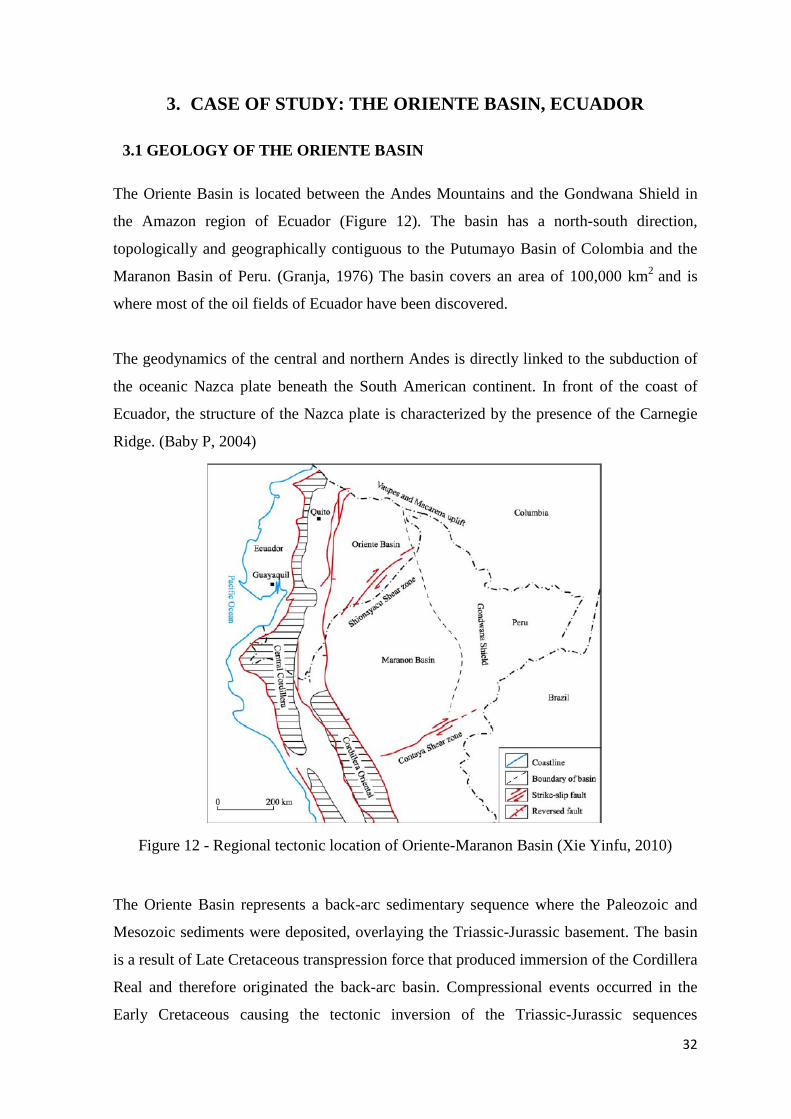
The Oriente Basin is located between the Andes Mountains and the Gondwana Shield in
the Amazon region of Ecuador (Figure 12). The basin has a north-south direction,
topologically and geographically contiguous to the Putumayo Basin of Colombia and the
Maranon Basin of Peru. (Granja, 1976) The basin covers an area of 100,000 km2 and is
where most of the oil fields of Ecuador have been discovered.
The geodynamics of the central and northern Andes is directly linked to the subduction of
the oceanic Nazca plate beneath the South American continent. In front of the coast of
Ecuador, the structure of the Nazca plate is characterized by the presence of the Carnegie
Ridge. (Baby P, 2004)
Figure 12 - Regional tectonic location of Oriente-Maranon Basin (Xie Yinfu, 2010)
The Oriente Basin represents a back-arc sedimentary sequence where the Paleozoic and
Mesozoic sediments were deposited, overlaying the Triassic-Jurassic basement. The basin
is a result of Late Cretaceous transpression force that produced immersion of the Cordillera
Real and therefore originated the back-arc basin. Compressional events occurred in the
Early Cretaceous causing the tectonic inversion of the Triassic-Jurassic sequences

33
throughout the basin. The deformation and structure of the traps and oil fields are the result
of the inversion of old faults linked to rift systems of the Triassic-Jurassic age. These faults
now reversed and steeply dipping, are mainly oriented NS or NNE-SSW. (Baby P, 2004)
The faults delineate three structural oil corridors with own characteristics (Figure 13):
• Subandino System (Weast Play)
• Sacha-Shushufindi System (Central Play)
• Capirón-Tiputini System (East Play)
Figure 13 - Oil structural corridors of Oriente Basin. (Modified from Baby, 2004)
The corridor Sacha-Shushufindi, shown in blue in figure 13, is a back arc basin controlled
by deep faults associated with a rift system developed during the Triassic-Jurassic. The
Sacha-Shushufindi play covers the most important fields of the country: Sacha,
Shushufindi and Libertador. At the north are the fields with light and medium oil, while at
the centre and south the oil turns from medium to heavy. Even if it is a mature play,
prospective is high because the traps are old; therefore any mapped structure has a good
probability of having oil.

34
The Capiron-Tiputini play, shown in green in figure 13, has normal listric faults
horizontally interconnected. The Capiron-Tiputini play is where the ITT and Pañacocha
fields are located. This structure has medium and heavy oil.
The Subandino play, shown in green in figure 13, has three important structures: The Napo
lifting in NNE-SSO direction, limited to the east and west by transpressive faults, the
Pastaza depression where the faults are more dispersed; and the Cutucu mountains where
the structures changes direction from N-S to NNW-SSE emerging the Triassic-Jurasic
Santiago and Chapiza formations. In the Subandino play is located the Bermejo field where
heavy and extra heavy oils are present.
3.1.2 DEPOSITIONAL ENVIRONMENT
The Early Cretaceous volcanic activity was followed by the marine sedimentation in the
Late Cretaceous. Continental sedimentation followed the Cretaceous depositions; Cenozoic
sediments took place along the axis of the back arc basin. Cenozoic and Mesozoic
sediments are preserved in the Ecuadorean fields. (Baldock, 1982) Figure 15 shows the
depositional environment along the region corresponding to the oil corridors previously
described.
Figure 14 – Paleogeography map of the Napo Formation, Oriente Basin
(J. Estupiñan R. M., 2010)

35
Figure 15 – Stratigraphy of the Oriente Basin (Dashwood M F, 1990)

36
3.1.1 STRATIGRAPHY OF ORIENTE BASIN
Well logging and seismic reflection have corroborated geological studies to get the
stratigraphy of the basin. The following main formations have been determined across the
Oriente Basin from bottom to surface: Hollin, Napo, Tena, Tiyuyacu, Orteguaza, Chalcana,
Arajuno and Chambira. In some areas the presence of a specific formation is more evident
than in others. Figure 14 shows the stratigraphy of the basin related to the geological
occurrence time.
There are several sets of potential source rocks in the Oriente Basin, among which the
Cretaceous Napo formation of the Mesozoic Era is the most important in the north of the
basin based on geochemical analysis of crude oil and source rock extraction; while in the
south of the basin oil comes from the Triassic-Jurassic Santiago formation.
The sandstone Cretaceous Napo formation is where most of the hydrocarbon has been
found in the fields of the country. In turn, Napo formation is composed of some layers
listed on table 2.
Table 2 – Napo formations sub-layers
Napo Formations Rock type Napo Upper Lutite
M1 Limestone M2 Limestone A Limestone
U upper Sandstone U lower Sandstone
Napo medium Lutite B Limestone
T upper Sandstone T lower Sandstone Basal T Sandstone
Napo lower Lutite

37
Within the Napo sedimentary rock formation there are two important reservoir units called
U and T sandstones. Those are composed of cyclic sequences of limestones, shales and
sandstones deposited on a low-energy shallow-marine platform controlled by sea level
changes. (White, 1995)
The depositional stage for the Napo T sandstone interval corresponds to sea level fall
during the Cretaceous Albian Age that created a major boundary and an erosive drainage
network after filled by incised valley sandstones during an early transgressive sea-level
rise.
The depositional stage of the Napo U sandstone interval corresponds to a later sea level
fall during the Cretaceous Cenomanian Age, resulted in another erosional sequence
boundary. Although similar in terms of environment of deposition, the sandstone members
are different in composition and maturity. Napo formation is the main producing reservoir
of the basin. It is composed of many formation units described on Table 2.
The braided river-delta sandstone called Hollin is other important formation of the basin.
This reservoir consists of thick-bed to massive white quartz sandstones, widely spread. It
mainly serves as a lateral migration pathway for hydrocarbons. Fields of this reservoir are
mainly distributed in the central and western parts of the Oriente Basin. (Marocco R, 1995)
The fluvial river sandstone Tena formation composed of massive quartz sandstones is
above the Napo formation, but is not well developed in the whole Oriente Basin.
Along the country the structure of the Napo reservoir varies from one point to another. In
figure 16 is summarized the stratigraphy sequence and geological occurrence time of the
entire Napo reservoir rock layers or also called litho-facies.
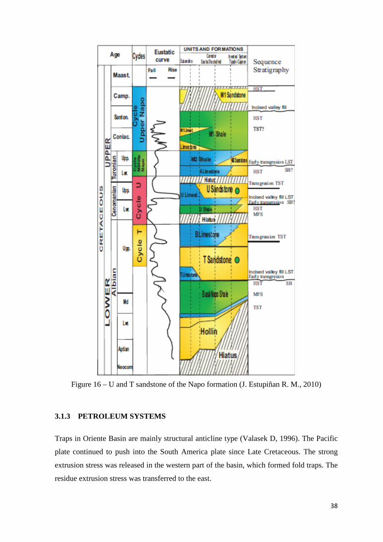
38
Figure 16 – U and T sandstone of the Napo formation (J. Estupiñan R. M., 2010)
3.1.3 PETROLEUM SYSTEMS
Traps in Oriente Basin are mainly structural anticline type (Valasek D, 1996). The Pacific
plate continued to push into the South America plate since Late Cretaceous. The strong
extrusion stress was released in the western part of the basin, which formed fold traps. The
residue extrusion stress was transferred to the east.
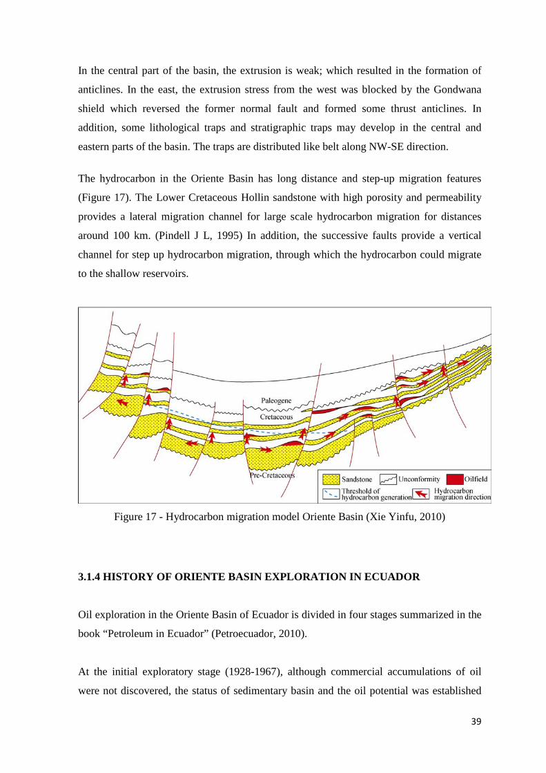
39
In the central part of the basin, the extrusion is weak; which resulted in the formation of
anticlines. In the east, the extrusion stress from the west was blocked by the Gondwana
shield which reversed the former normal fault and formed some thrust anticlines. In
addition, some lithological traps and stratigraphic traps may develop in the central and
eastern parts of the basin. The traps are distributed like belt along NW-SE direction.
The hydrocarbon in the Oriente Basin has long distance and step-up migration features
(Figure 17). The Lower Cretaceous Hollin sandstone with high porosity and permeability
provides a lateral migration channel for large scale hydrocarbon migration for distances
around 100 km. (Pindell J L, 1995) In addition, the successive faults provide a vertical
channel for step up hydrocarbon migration, through which the hydrocarbon could migrate
to the shallow reservoirs.
Figure 17 - Hydrocarbon migration model Oriente Basin (Xie Yinfu, 2010)
3.1.4 HISTORY OF ORIENTE BASIN EXPLORATION IN ECUADOR
Oil exploration in the Oriente Basin of Ecuador is divided in four stages summarized in the
book “Petroleum in Ecuador” (Petroecuador, 2010).
At the initial exploratory stage (1928-1967), although commercial accumulations of oil
were not discovered, the status of sedimentary basin and the oil potential was established

40
based on the presence of surface springs and few exploratory works. After initial analysis
the sediment thickness, potential existence of a source rock and sandstones with highly
potential of reservoir rock were discovered. The structure derived from the Andean
evolution was defined. The end of this first exploration effort was concluded by
discovering oil in one well at the Basal Tena reservoir.
The second stage (1967-1972), the Oriente was confirmed as an oil basin with the
discovery of the biggest fields: Lago Agrio, Shushufindi, Sacha and Auca. These fields
incorporated the greatest oil reserves of the country.
Third stage (1972-1982), was when exploratory activity was developed. State-owned and
international oil companies discovery the field Libertador, which is the fourth bigger in the
basin.
The fourth stage (after 1983), is when exploratory maturity is achieved. This stage was
characterized by a decrease in the rate of exploration success, by decreasing the size of the
exploration prospects and by an increase in the density of the discovered crude
(Rivadeneira M, 2004). In this stage the discovery of the small marginal fields among
which Singue was discovered. The drilling of the well Singue-1 was done in 1990 and
confirmed the existence of the field as an independent oil reservoir.
The Oriente Basin in Ecuador had been explored for more than 50 years, now it is seem to
be into the maturity stage. Seismic coverture of almost all the geography had been
obtained, an important number of exploratory wells and geological studies allow an
important knowledge of the reservoir such as the tectonic structure, stratigraphic
architecture and oil producing systems is available to assess the study of new fields in the
region. (Petroecuador, 2010)

41
4. METODOLOGY
To estimate the production potential of the field Singue and meet the objectives of this
dissertation the methodology used by the author is described in this chapter.
The first step is the analysis of the data available to understand the current status of the
field. The field has one well named Singue-1 that was producing oil from 1991 to
1997. Another exploratory well named Alama-1 that was drilled on 1984 but was water
saturated. The information available is listed:
o General information of the field.
o Geological information of the basin.
o Core samples results and bio-stratigraphic report of the well Singue-1.
o PVT analysis results of the fluid and production history of the well Singue-1.
o Raw 2D seismic surveys of the area.
o Raw well logs of Singue-1 and Alama-1.
The second step is the evaluation of the formation based on the well logging
interpretation of the available logs of Singue-1 in the software Interactive Petrophysics
(IP). With this information is possible to define the possible reservoirs in the field and
define the properties of them. The input parameters required for the program are the
“.las” files of each well. The interpretation procedure for the interpretation in IP is
detailed later on this chapter.
The third step is the seismic interpretation in Petrel to then integrate the results with the
log interpretation results and the available information described on section 4.1 to find
the boundaries of the reservoir. The process will give a better idea of the field potential.
The input parameters for Petrel are the seismic surveys “.sgy” files and the “.las” well
logs files. The procedure for the integration of logs and seismic data, as well as the
interpretation methodology is detailed later on this chapter.
Finally, the step four is the calculation of the remaining oil reserves in the field based
on previous stages results.
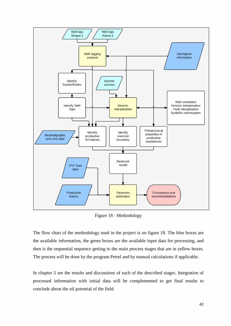
42
Figure 18 - Methodology
The flow chart of the methodology used in the project is on figure 18. The blue boxes are
the available information, the green boxes are the available input data for processing, and
then is the sequential sequence getting to the main process stages that are in yellow boxes.
The process will be done by the program Petrel and by manual calculations if applicable.
In chapter 5 are the results and discussions of each of the described stages. Integration of
processed information with initial data will be complemented to get final results to
conclude about the oil potential of the field.
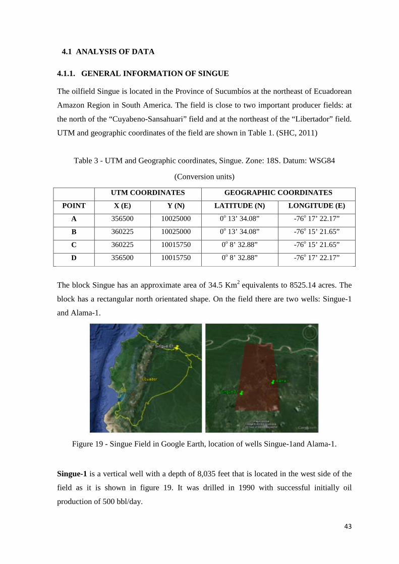
43
4.1 ANALYSIS OF DATA
4.1.1. GENERAL INFORMATION OF SINGUE
The oilfield Singue is located in the Province of Sucumbíos at the northeast of Ecuadorean
Amazon Region in South America. The field is close to two important producer fields: at
the north of the “Cuyabeno-Sansahuari” field and at the northeast of the “Libertador” field.
UTM and geographic coordinates of the field are shown in Table 1. (SHC, 2011)
Table 3 - UTM and Geographic coordinates, Singue. Zone: 18S. Datum: WSG84
(Conversion units)
UTM COORDINATES GEOGRAPHIC COORDINATES
POINT X (E) Y (N) LATITUDE (N) LONGITUDE (E)
A 356500 10025000 0o 13’ 34.08” -76o 17’ 22.17”
B 360225 10025000 0o 13’ 34.08” -76o 15’ 21.65”
C 360225 10015750 0o 8’ 32.88” -76o 15’ 21.65”
D 356500 10015750 0o 8’ 32.88” -76o 17’ 22.17”
The block Singue has an approximate area of 34.5 Km2 equivalents to 8525.14 acres. The
block has a rectangular north orientated shape. On the field there are two wells: Singue-1
and Alama-1.
Figure 19 - Singue Field in Google Earth, location of wells Singue-1and Alama-1.
Singue-1 is a vertical well with a depth of 8,035 feet that is located in the west side of the
field as it is shown in figure 19. It was drilled in 1990 with successful initially oil
production of 500 bbl/day.

44
Alama-1 is a vertical well with a depth of 8054 feet. It is the closest well to Singue-1 and
was drilled in 1984 for appraisal development of the region. The well was dry of oil,
namely water saturated. The information of this well is helpful to understand the geology
of the region. The summary of general information of the wells is on table 4.
Table 4 - General Information of the wells. Singue-1 and Alama-1.
SINGUE -1 ALAMA -1
Well location (Geographical
Coord):
Long: -76° 16' 59.45" E Long: -76° 15' 35.85" E
Lat: 00° 09' 27.46" N Lat: 00° 09' 55.04" N
Well location in UTM Zone
(18S):
X (east): 357086.9688 X (east): 359685.9063
Y (north): 10017429.0000 Y (north):
10018258.0000
Altitude of the terrain: 806 ft. 898 ft..
Depth of the well: 8035 ft. 8054 ft.
Geological position of the well: Centre of the anticline Top of anticline
Production tests: Produced Napo U lower Water saturated
Status of the well: Abandoned 1997 Dry
4.1.2. GEOLOGICAL STRUCTURE OF THE BASIN
The field is located in the Oriente Basin of Ecuador, which was result of transpressive
effort of the Late Cretacius that generated the emergence of the Cordillera Real and the
formation of the back arc basin and Ecuadorean Andes. Singue Field is located to the end
of Capirón system more NNW-Tiputini system orientated, which corresponds to an
extended inverted basin, currently structured by listric faults that are connected on a
horizontal level off overall. Additional information of the Oriente Basin can be found in
chapter 3.
The operator company at the time defined the geological structure of the field as an
anticline NS direction that was discovered with the well Singue-1. The length of the
structure is of approximately 1.2 Km and the width is approximately 0.9 Km. resulting an
anticline area of approximately 1 Km2. (Petroproduccion, 1990)

45
4.1.3. BIOSTRATIGRAPHY ANALYSIS OF SINGUE-1
The biostratigraphy analysis is the study of the micro-paleontological elements present in
rock samples taken during the drilling. The results give an idea of the sedimentary deposit
environment of each sample. Then it is assigned to a geological time of occurrence that has
specific characteristics in each rock layer. And then is possible to identify to which
formation the core belongs. The biostratigraphy analysis of Singue-1 was done with 37
reservoir samples taken from the depth of 4566 to 7900 ft. Table 5 shows the results of the
analysis. (Petroproduccion, 1991)
Table 5 - Biostratigraphy results of Singue-1
Depth interval (ft)
Sedimentary
Depositional
Environment
Geologic Time (Age) Formation that
represent
4566 – 5316 Shallow marine Oligocene Orteguaza
5379 – 6822 Shallow marine Palaeogene Tiyuyacu
6885 – 7109 Transitional Upper cretasic Tena
7210 – 7520 Continental marine Santonian Napo
7610 – 7830 Continental marine Turonian medium – Santonian Napo
7890 – 7900 Continental marine Turonian medium Napo
4.1.4. CORE SAMPLE ANALYSIS OF SINGUE-1
Three core samples of 30 ft. were analysed in laboratory to determine the percentage of
uranium, potasium and thorium presented in the formation based on the gamma radiation
of these elements in each sample. This study enforces the identification of the sedimentary
rock and depositional environments that represent. The results of the core sample analysis
of Singue-1 are shown in Table 6. (Petroproduccion, 1991)
Table 6 - Singue 1 Core samples tests
Core sample
interval (ft)
Uranium
(U)
Potasium
(K)
Thorium
(Th)
Depositional
environment
Formation that
represent
7684 – 7714 3 ppm 2.6 % 12 ppm Marine and continental Napo U upper
7760-7790 3 ppm 2.6 % 12 ppm Marine Napo U lower
7891-7921 3 ppm 2.6 % 12 ppm Marine and continental Napo T
46
4.1.5. PVT ANALYSIS OF SINGUE-1
Pressure-volume-temperature (PVT) laboratory analysis was made with two samples of the
fluid of the Napo U sandstone formation (7744-7760 ft) of the well Singue-1.
(Petroproduccion, 1994)
Bubble point was calculated at ambient temperature. Then the sample was taken to a high
pressure cell at the bottom hole temperature of 206oF. At this temperature the sample
reached the bubble point at a pressure of 550 psi and released 162 ft3 of gas per residual oil
barrel at 14.7 psi and 60 oF. The volumetric factor is 1.2289 barrels of saturated oil per
barrel of residual oil at 60oF. The residual oil at 60oF has a API gravity of 24.4 and at
206oF it has a density of 0.9587 gr/cc. Viscosity of the fluid was determined at bottom hole
temperature of 206oF, obtaining values of 3.20 cP at saturation pressure and 4.08 cP at
atmospheric pressure. Additionally, some gas parameters were calculated at bubble point
such as compressibility (Z), gas volumetric factor (Bg) and solubility (RS). Complete
results are shown in table 7.
Table 7 - Volumetric information Napo U sanstone of Singue-1
General Information Formation Napo U sandstone
Interval 7744-7760 ft
Sample height (Ho) 16 ft
Water saturation (Sw) 0.3%
Bottom hole temperature 206 oF
PVT results Saturation pressure at 206 oF 550 psi
Thermic expansion of
Saturated oil
Volume at 206 oF and 5000 psi 0.0533
Volume at 82 oF and 5000 psi 1.0661
Saturated oil
(550psi, 206 F)
Gas-Oil ratio (GOR) 162
Volumetric factor (Bo) 1.2289
Density 0.7857 (lbs/bbl)
Specific volume 0.0204
Viscosity 3.20 cP
Residual oil
API gravity at 60 oF 24.4
Density at 206 oF 0.9587 (gr/cc)
Viscosity at 206 oF 4.08
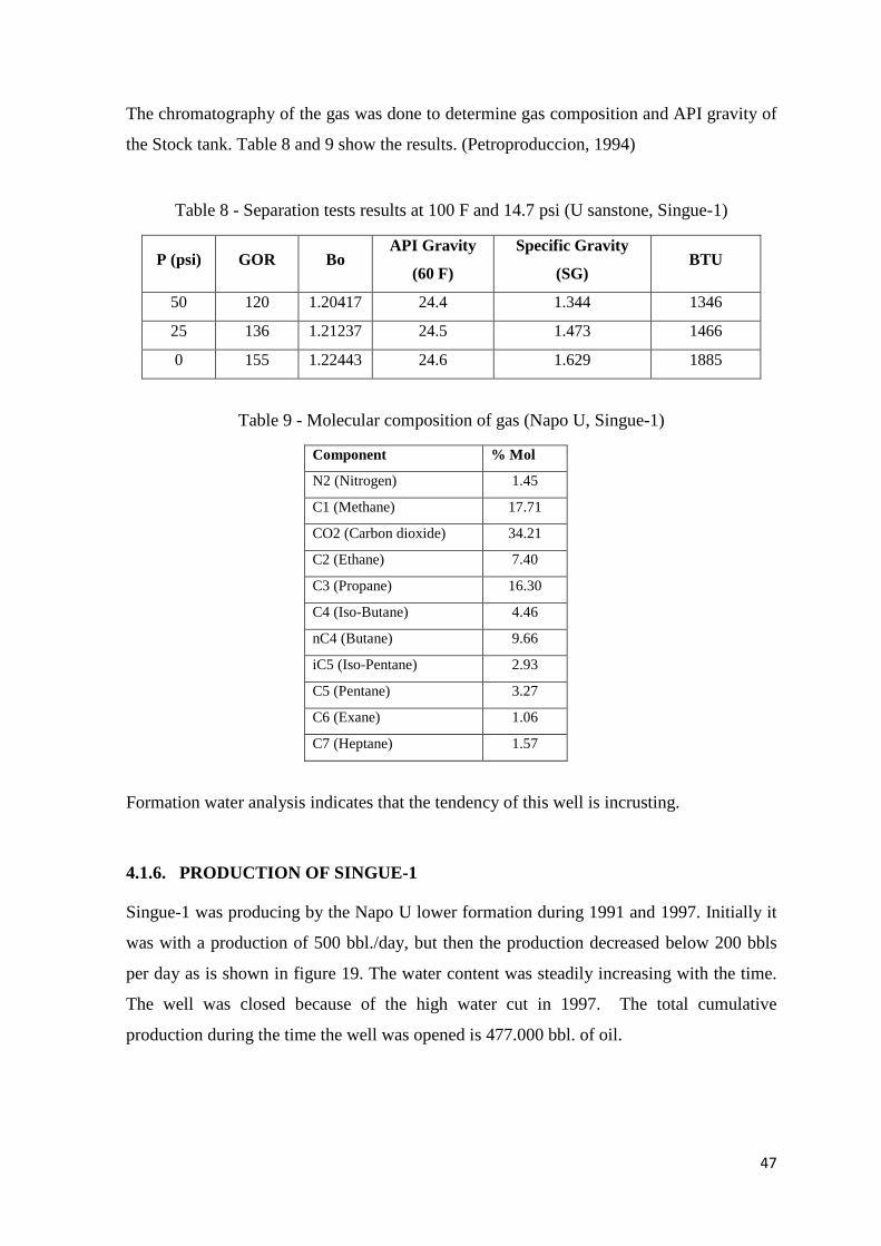
47
The chromatography of the gas was done to determine gas composition and API gravity of
the Stock tank. Table 8 and 9 show the results. (Petroproduccion, 1994)
Table 8 - Separation tests results at 100 F and 14.7 psi (U sanstone, Singue-1)
P (psi) GOR Bo API Gravity
(60 F)
Specific Gravity
(SG) BTU
50 120 1.20417 24.4 1.344 1346
25 136 1.21237 24.5 1.473 1466
0 155 1.22443 24.6 1.629 1885
Table 9 - Molecular composition of gas (Napo U, Singue-1)
Component % Mol
N2 (Nitrogen) 1.45
C1 (Methane) 17.71
CO2 (Carbon dioxide) 34.21
C2 (Ethane) 7.40
C3 (Propane) 16.30
C4 (Iso-Butane) 4.46
nC4 (Butane) 9.66
iC5 (Iso-Pentane) 2.93
C5 (Pentane) 3.27
C6 (Exane) 1.06
C7 (Heptane) 1.57
Formation water analysis indicates that the tendency of this well is incrusting.
4.1.6. PRODUCTION OF SINGUE-1
Singue-1 was producing by the Napo U lower formation during 1991 and 1997. Initially it
was with a production of 500 bbl./day, but then the production decreased below 200 bbls
per day as is shown in figure 19. The water content was steadily increasing with the time.
The well was closed because of the high water cut in 1997. The total cumulative
production during the time the well was opened is 477.000 bbl. of oil.
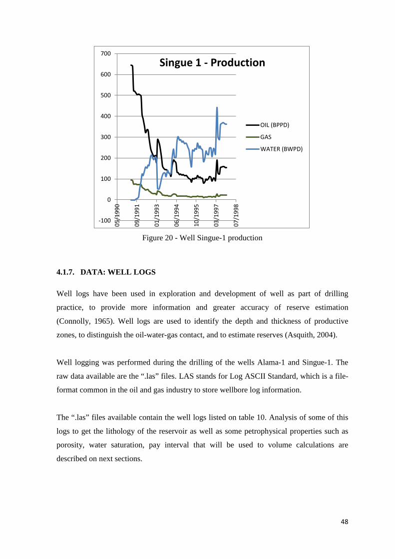
48
Figure 20 - Well Singue-1 production
4.1.7. DATA: WELL LOGS
Well logs have been used in exploration and development of well as part of drilling
practice, to provide more information and greater accuracy of reserve estimation
(Connolly, 1965). Well logs are used to identify the depth and thickness of productive
zones, to distinguish the oil-water-gas contact, and to estimate reserves (Asquith, 2004).
Well logging was performed during the drilling of the wells Alama-1 and Singue-1. The
raw data available are the “.las” files. LAS stands for Log ASCII Standard, which is a file-
format common in the oil and gas industry to store wellbore log information.
The “.las” files available contain the well logs listed on table 10. Analysis of some of this
logs to get the lithology of the reservoir as well as some petrophysical properties such as
porosity, water saturation, pay interval that will be used to volume calculations are
described on next sections.
-100
0
100
200
300
400
500
600
700
05/1
990
09/1
991
01/1
993
06/1
994
10/1
995
03/1
997
07/1
998
Singue 1 - Production
OIL (BPPD)
GAS
WATER (BWPD)
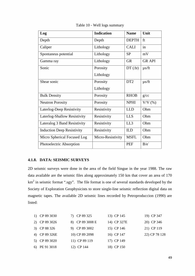
49
Table 10 - Well logs summary
Log Indication Name Unit
Depth Depth DEPTH ft
Caliper Lithology CALI in
Spontaneus potential Lithology SP mV
Gamma ray Lithology GR GR API
Sonic Porosity
Lithology
DT (Δt) µs/ft
Shear sonic Porosity
Lithology
DT2 µs/ft
Bulk Density Porosity RHOB g/cc
Neutron Porosity Porosity NPHI V/V (%)
Laterlog-Deep Resistivity Resistivity LLD Ohm
Laterlog-Shallow Resistivity Resistivity LLS Ohm
Lateralog 3 Band Resistivity Resistivity LL3 Ohm
Induction Deep Resistivity Resistivity ILD Ohm
Micro Spherical Focused Log Micro-Resistivity MSFL Ohm
Photoelectric Absorption PEF B/e-
4.1.8. DATA: SEISMIC SURVEYS
2D seismic surveys were done in the area of the field Singue in the year 1988. The raw
data available are the seismic files along approximately 150 km that cover an area of 170
km2 in seismic format “.sgy”. The file format is one of several standards developed by the
Society of Exploration Geophysicists to store single-line seismic reflection digital data on
magnetic tapes. The available 2D seismic lines recorded by Petroproduccion (1990) are
listed:
1) CP 89 3030
2) CP 89 3026
3) CP 88 326
4) CP 89 326E
5) CP 89 3020
6) PE 91 3018
7) CP 89 325
8) CP 89 3008 E
9) CP 89 3002
10) CP 89 2098
11) CP 89 119
12) CP 144
13) CP 145
14) CP 327E
15) CP 146
16) CP 147
17) CP 149
18) CP 150
19) CP 347
20) CP 346
21) CP 119
22) CP 78 128

50
Recording Equipment:
• Geophones and a portable register MDS-16, recording format SEG-B.
• The field parameters used were 40m in between points, shoots each 80m, depth 15 to
20 m with 2 pound of explosive.
• The receptor had 120 channels located in between channels 60 and 61 the farthest
channel was at 2400 m of the origin.
• 9 geophones were used per channel. The line CP-89-326-E has a coverture of 2.4% and
the shots were done each 40 m. (Petroproduccion, 1990)
Initial interpretations determined that Singue structure had high possibilities of being a
reservoir. The exploratory well Singue-1was drilled in the line CP 89 326E at the shooting
point 295. Re-process of the lines to assess in the remaining oil reserves will be described
in next sections.
4.2 WELL LOGGING ANALYSIS
The aim is to process and interpret the well logs of the well Singue-1 and Alama-1 to
determine the stratigraphy and petro-physical characteristics of the sandstones. The study
has been carried through qualitative and quantitative analysis by the programs Interactive
Petrophysics (IP).
The analysis includes determination of permeable rock zones and within each formation
calculation of formation pay thickness, porosity and fluid saturation. Other parameters
such as shale volume of each formation must be determined for this purpose.
The methodology for each stage in the program IP is described below:
WELL LOG INTERPRETATION TO IDENTIFY RESERVOIR ROCK 4.2.1
a) Create a project in IP and create the wells Singue-1 and Alama-1, define general
specifications such as well head position and import the well logs “.las” files into
each well.

51
b) Make a quality check of the logs, to be sure the data is in the corresponding units
and ranges.
c) Run the Basic Log Interpretation process and plot the results in the range of interest
for each well.
d) Interpret GR, SP, RHOB, NPHI, CALIPER and RESISTIVITY logs to identify the
lithology of the well and permeable formations.
e) Pick the well tops of each identified permeable formation.
f) Compare results with expected stratigraphy of the region presented on chapter 3
and with the bio-stratigraphic and core sample report presented on chapter 4.1.
WELL CORRELATION 4.2.2
a) Using IP analyse well logs to identify the well tops of each formation picked in the
area of interest that is between 7200 and 8100 ft.
b) Use the well correlation process to correlate the logs for the available wells to
identify if there are changes in the stratigraphy in the two available wells.
c) Plot the well correlation obtained.
PETROPHYSICAL ANALYSIS 4.2.3
Interactive Petrophysics have special modules to perform well log interpretation. The
methodology includes: calculation of clay volume, porosity, water saturation and Net Pay
thickness of each formation. The results are required for the volumetric calculation of oil in
place. The well log interpretation is based on the Interactive Petrophysics Help document
procedure (Senergy Software Ltd., 2011). The used modules are: Basic Interpretation
module, Shale volume module, Porosity and water saturation module, Cutoff and
Summation module.
The basic module is a faster way of processing the data. The other three modules use more
complex algorithms and are run together to get more accurate results. Both ways were
developed in this project. Methodology of each module used for the interpretation of the
logs of Singue-1 contained in the “.las” file is described below.

52
Basic Log Interpretation
a) In the IP project open the Basic Log Analysis module.
b) Define Density, Sonic or Neutron/density logs as input for Porosity calculations.
c) Define GR as input for Clay Volume Calculations.
d) Define the resistivity curve as input for Water Saturation calculation.
e) Define the rock zones previously found.
f) Select the clay volume calculation method and define GR clean (minimum value in
clean non shaley intervals) and GR clay (maximum value in shale intervals) values. In
this case is used GR method, Gr clean and Gr are selected interactively from the
curves.
g) Clay Volume (Vcl) is calculated and plotted using the equation:
𝑉𝑐𝑙 = 𝐺𝑟𝑙𝑜𝑔−𝐺𝑟𝑐𝑙𝑒𝑎𝑛𝐺𝑟𝑐𝑙𝑎𝑦−𝐺𝑟𝑐𝑙𝑒𝑎𝑛
h) Select the porosity calculation model from Density, Sonic or Neutron/Density. In this
case will be used the Density model. Set the parameters: Rhomatrix = 2.65 for
sandstones, Rhofluid = 1 g/cc for fresh water, Rhoclay is the density reading of the log in
the shale interval in this case is 2.626. Vcl is the caly volume calculated.
i) Porosity (Phi) is calculated and plotted using the equation:
𝑃ℎ𝑖 = 𝑅ℎ𝑜𝑚𝑎𝑡𝑟𝑖𝑥 − 𝑅ℎ𝑜𝑏 − 𝑉𝑐𝑙 × (𝑅ℎ𝑜𝑚𝑎𝑡𝑟𝑖𝑥 − 𝑅ℎ𝑜𝑐𝑙𝑎𝑦)
(𝑅ℎ𝑜𝑚𝑎𝑡𝑟𝑖𝑥 − 𝑅ℎ𝑜𝑓𝑙𝑢𝑖𝑑)
j) Select the model used for water saturation calculation from Archie, Simand or
Indonesian models. In clean rock select Archie, in shaley sands the Simandoux or
Indonesian equations will make corrections for shale in the rock and give better results.
In this case is used Archie method with the parameters: Rwformation temperature = 0.1 ohm,
Archie factor a=1, m=2 and n=2. Those parameters also could be picked from
porosity/resistivity curves. Rt is the value from the log.
k) Water saturation is calculated and plotted using the Archie’s equation:
𝑆𝑤𝑈 = (𝑎 × 𝑅𝑤
𝑃ℎ𝑖𝑚 × 𝑅𝑡)1/𝑛
l) Analyse the result curves: porosity (PHI), water saturation (Sw), bulk volume water
(BVW), clay volume (VCL), apparent water resistivity (Rwapp).

53
Clay Volume Interpretation
a) In the IP project open the Clay Volume interpretation process. Input as single clay
indicators the gamma ray (GR), resistivity (ILD) and as double clay indicators the
density/neutron (RHOB/NPHI) logs imported from the “.las” file of the well. Define
the caliper log as bad hole indicator.
b) Run the simulation to get minimum clay volume (VCL) and average clay volume
(VCLAV) and the corresponding plots.
c) Define the zones and select the method used for each clay indicator:
The Gamma Ray clay indicator (VclGr) is set to the linear as in the basic
interpretation module.
The resistivity is set as linear. 𝑍 = 𝐺𝑟𝑐𝑙𝑒𝑎𝑛𝑅𝑡
× 𝑅𝑐𝑙𝑒𝑎𝑛−𝑅𝑡𝑅𝑐𝑙𝑒𝑎𝑛−𝑅𝑐𝑙𝑎𝑦
The sonic density work on the principle of defining a clean line and a clay point.
The clay volume is calculated as the distance the input data falls between the clay
point and the clean line.
d) Analyse the input curves, change limits of maximum and minimum parameters for
each method if it is required.
e) Interpret and discuss the obtained results for VCL and VCLAV in each formation.
Porosity and Water Saturation Interpretation
a) Porosity and water saturation is done under the interpretation menu, porosity and water
saturation analysis.
b) Link the module to the clay results.
c) Define the porosity model and saturation equation. In this case is used the Density
model for porosity and the Archie equation for water saturation.
If the density porosity model is selected, then porosity is calculated as follows:
54
Where the values are picked from the input curves,
ρma= Matrix density ρb = Input bulk density log ρcl = Wet clay density ρfl =Filtrate density, calculated in 2 or entered as a parameter ρHyAp = Apparent hydrocarbon density, calculated in.4, entered as a parameter Vcl = Wet clay volume Sxo = Flushed zone water saturation
Archie water saturation equation is defined by:
Where, a = 1, n = 2, m =2.
d) IP assumes that any neutron curve entered is in Limestone matrix units. If this is not
the case, then the curve should be converted to Limestone porosity units.
e) Generate the temperature curve. Temperature is 206 F from PVT data.
f) Run the simulation to get the plots of porosity and water saturation for each zone.
Results include: porosity (PHI), water saturation (Sw), flushed zone water saturation
(Sxo), matrix density (RHOMA), hydrocarbon density (RHOHY) and wet and dry clay
volumes (VWCL & VDCL).
g) Modify the input parameters if necessary interactively from the plots, refer to me
Interactive petrophysics help manual.
h) Analyse results for each formation.
Cutoffs and Summation
The Cut-offs and Summation module allows you to interactively define Net Reservoir and
Net Pay cut-off criteria and zones, and to calculate the average petrophysical properties of
porosity, clay volume and water saturation for each zone.
a) Open Cut-offs and Summation under interpretation menu in IP.
b) Define the input curves: Clay Volume (VCL), Porosity (PHI) and Water saturation
(Sw), obtained in previous sections. .

55
c) Select the averaging method for each input curve. Available methods in selecting the
averaging method for creating a continuous attribute are:
- Arithmetic (Typically used for attributes such as porosity, saturation and net/gross
because these are additive variables. The arithmetic mean is only correct for
horizontal permeability that is constant within each layer).
- Harmonic (Gives the effective vertical permeability if the reservoir is layered with
constant permeability in each layer. The harmonic mean works well with log
normal distributions. Used for permeability because it is sensitive to lower values.
Only positive values may be used with this method).
- Geometric (Normally a good estimate for permeability if it has no spatial
correlation and is log normally distributed. The geometric mean is sensitive to
lower values, which will have a greater influence on results. Only positive values
may be used with this method).
In this case was used the arithmetic method with following equations:
• Average porosity:
• Average water saturation:
• Average Clay volume:
• Extra curve arithmethic average:

56
Where, i = ith input value, hi = height input interval, n = number of samples.
d) The default Cut-offs values are used to initialize the calculations
e) Run the simulation to get the Reservoir and Pay plots.
f) Check the Cutoff parameters: Zone Depths, Reservoir Cutoffs, Pay Cutoffs, Additional
Cutoffs,. Change any parameter in the parameters screen if is necessary.
g) Analyse results and plots that include Reservoir Results, Pay Results and Additional
Results curves with parameters which include Gross Interval, Net interval, Net/Gross
ratio, Average porosity and Average water saturation in the reservoir and in the Net
Pay intervals.
4.3 SEISMIC INTERPRETATION
The aim is to process the seismic raw data available in Petrel to get the boundaries of the
reservoir. Integration of the well logs with the picked well tops with the seismic data in
time is the initial stage. Then a model for the interpretation of horizons and faults has to be
done to get the boundaries and area of the reservoir.
a) Create a Petrel project with the coordinate reference system of the data (CRS) that is
located in the UTM zone 18S.
b) Create a well folder with the wells Singue-1 and Alama-1, define well head position,
well path and import the well logs “.las” files with the available logs for each well.
c) Open the well section window with each well and display the logs. Identify the well
tops based on the obtained data of the previous section.
d) Import the 2D seismic lines available.
WELL TIE 4.3.1
Well tie process relates well logs with seismic surveys. The procedure is done following
the Petrel 2010 Manual (Schlumberger, 2011).
a) Under well tie process in Petrel use the sonic log to create the sonic despiked log.
b) Do the sonic calibration to transform the well tops data from depth to TWT (two
way time data) to relate logs with seismic data by the wavelet extraction process.

57
c) Create the synthetic seismogram.
d) Display well tops table with depth and time.
HORIZON INTERPRETATION 4.3.2
After having the synthetic seismogram and well tops in time horizon interpretation could
be done. Each horizon corresponds to a well top, namely the top of a facie.
a) Under seismic interpretation process of Petrel open the seismic data and well tops
(TWT), each well top correspond to a seismic horizon in time domain.
b) In the interpretation window open one by one the seismic lines and start horizon
interpretation for the 5 formations: Napo U up, U low, T up, T low and Basal T.
Use manual and 2D auto-tracking tool of Horizon interpretation.
c) A folder with the horizons is created, and the horizons could be displayed in the 2D
or 3D window.
FAULT INTERPRETATION 4.3.3
a) Under seismic interpretation process, activates fault interpretation tool.
b) In the interpretation window open one by one the seismic lines and start fault
interpretation, use manual lines to identify faults.
c) Follow the identified faults in all the seismic sections.
d) A folder with the faults will be created.
BOUNDARY IDENTIFICATION 4.3.4
a) From the interpreted horizons create a surface under make/edit surfaces process.
b) Input interpreted horizon.
c) Select the algorithm used. In this case the default convergent interpolation is used.
d) Define the geometry of the field.
e) Execute the process. Surfaces for each horizon are being created.
f) Create a velocity model based on the manual (Schlumberger, 2011), use the created
surfaces and the well tops as input data. It will be used to do domain conversion
(time-depth) of any required data.
g) Convert the surfaces, horizons and faults to depth domain.

58
h) Under the operations tab of each surface variogram maps for each surface could be
created to visualize time/depth relations or properties of each surface.
i) Using the surfaces and faults define the boundary of the reservoir.
j) Use area to volumetric calculations.
4.2 RESERVES ESTIMATION
a) Calculate the STOOIP for each formation
The volumetric method used for initially oil in place calculation (STOIIP) is based on equation 1 mentioned in chapter 2.
STOIIP (STB) = 7758 × 𝑉𝑏 × Φ × (1 − Sw)
Bo
Where,
Vb = Area x thickness of the net pay
A = Area (acres) from seismic interpretation
th = Thicknes of net pay (ft) from well log interpretation
Φ = Average rock porosity (decimal) from well log interpretation
Sw = Average water saturation (decimal) from well log interpretation
Bo = Formation volume factor from PVT data
b) Calculate the initial reserves for each formation.
The initial reserves are calculated using the equation 2 mentioned in chapter 2:
Recorvable oil (bbl) = STOIIP × RF
Where,
RF = Recovery factor (approximate 25% for sandstones)
c) Calculate remaining reserves for each formation.
The remaining reserves are calculated using the equation:
Remanent reserves (bbls) = Recorvable oil – Production
Where, Production is the historical production of Singue-1
d) Add all the results to find the remaining oil in the field.
e) Discuss the results
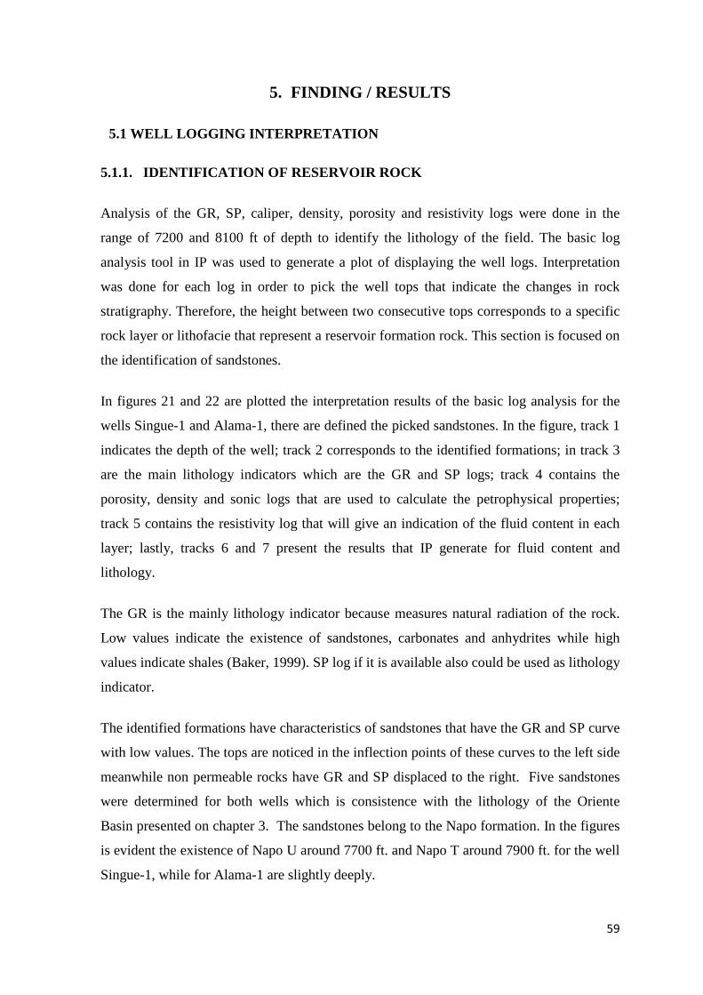
59
5. FINDING / RESULTS
5.1 WELL LOGGING INTERPRETATION
5.1.1. IDENTIFICATION OF RESERVOIR ROCK
Analysis of the GR, SP, caliper, density, porosity and resistivity logs were done in the
range of 7200 and 8100 ft of depth to identify the lithology of the field. The basic log
analysis tool in IP was used to generate a plot of displaying the well logs. Interpretation
was done for each log in order to pick the well tops that indicate the changes in rock
stratigraphy. Therefore, the height between two consecutive tops corresponds to a specific
rock layer or lithofacie that represent a reservoir formation rock. This section is focused on
the identification of sandstones.
In figures 21 and 22 are plotted the interpretation results of the basic log analysis for the
wells Singue-1 and Alama-1, there are defined the picked sandstones. In the figure, track 1
indicates the depth of the well; track 2 corresponds to the identified formations; in track 3
are the main lithology indicators which are the GR and SP logs; track 4 contains the
porosity, density and sonic logs that are used to calculate the petrophysical properties;
track 5 contains the resistivity log that will give an indication of the fluid content in each
layer; lastly, tracks 6 and 7 present the results that IP generate for fluid content and
lithology.
The GR is the mainly lithology indicator because measures natural radiation of the rock.
Low values indicate the existence of sandstones, carbonates and anhydrites while high
values indicate shales (Baker, 1999). SP log if it is available also could be used as lithology
indicator.
The identified formations have characteristics of sandstones that have the GR and SP curve
with low values. The tops are noticed in the inflection points of these curves to the left side
meanwhile non permeable rocks have GR and SP displaced to the right. Five sandstones
were determined for both wells which is consistence with the lithology of the Oriente
Basin presented on chapter 3. The sandstones belong to the Napo formation. In the figures
is evident the existence of Napo U around 7700 ft. and Napo T around 7900 ft. for the well
Singue-1, while for Alama-1 are slightly deeply.

60
Napo U is divided in two layers: U up and U low. For the first one the GR and SP logs are
not so steady, which means could be composed by other non-permeable rock elements.
The Napo U low has the most steady sandstone GR response for both wells. Below Napo
U low is evident the existence of a non-permeable rock that could be shale or a low
porosity limestone. Then is the Napo T formation that is divided in other three sub-layers:
T up, T low and T Basal. Napo T up shows steady sandstones responses to the GR. In the
border with the Napo T low the signal has drops, meaning the sandstone is mixed with
non-permeable rocks, decreasing the possibility of Napo T low to be a good permeable
rock. In Napo T Basal the signal is steady again.
Figure 21 - Singue-1 basic log interpretation. Lithology and well tops

61
Figure 22 - Alama-1 basic log interpretation. Lithology and well tops.
The sonic and caliper logs show a steady line in the sandstone region, that is a good
indicator of permeable rock. The density and neutron porosity log are together in the
sandstones regions which is another good indicator of liquid fluid content.
The analysis of the resistivity curves gives an indication of the presence of oil or water. In
the upper side of the Singue-1 in the Napo U low, the response to the right with high
resistivity values indicates the existence of oil. In the rest of the curves the log is not so

62
pronounced, it indicates the presence of water. In the well Alama-1 the resistivity response
is low, which indicates major presence of water along the facie.
The two tracks at the end show the automatic response of the software to porosity and
lithology analysis. In track 6 is shown the porosity curve and fluid content, red is for oil
and blue is for water. This information contributes to define that in Singue-1 the selected
sandstones have hydrocarbons. This does not occur in Alama-1, where responses give
highly indication of water content. This demonstrates the information that the well was oil
dry when it was drilled.
The final track shows the distribution of rock and porosity. In Singue-1 is evident the
sandstone that is yellow in all the identified formations. Napo U low is the one with
constant porosity mean value around 24%. This formation is the most probable to have
hydrocarbon. Napo U up, T up and Basal are the formations that are likely to have
petroleum but in less amount. Napo U up is the sandstone that shows very low probability
of having hydrocarbon.
In general for these first results the formation Napo is composed of sandstones but mixed
with other non-permeable rocks that change their properties and thus the probability of
having hydrocarbon content. The results obtained are summarized in table 11 and
correspond to the lithofacies of the Napo formation: Napo U up, Napo U low, Napo T up,
Napo T low and Napo Basal T.
Table 11 - Well tops from well log interpretation
SINGUE -1 ALAMA-1
Formation top Rock type Top (ft) Bottom (ft) Top (ft) Bottom (ft)
Napo U up Sandstone 7684 7742 7762 7831
Napo U low Sandstone 7742 7857 7830 7914
Napo T up Sandstone 7884 7981 7949 8036
Napo T low Sandstone 7981 8007 8036 8053
Napo Basal T Sandstone 8007 8051 8053 8102
Each formation top was assigned to a sandstone formation based on the regional
stratigraphy of the Oriente Basin described in Chapter 3. Tying this information with the
biostratigraphy and core samples data, could be concluded that the facies belong to the
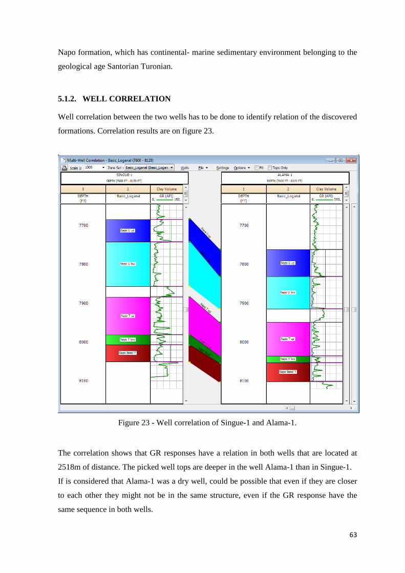
63
Napo formation, which has continental- marine sedimentary environment belonging to the
geological age Santorian Turonian.
5.1.2. WELL CORRELATION
Well correlation between the two wells has to be done to identify relation of the discovered
formations. Correlation results are on figure 23.
Figure 23 - Well correlation of Singue-1 and Alama-1.
The correlation shows that GR responses have a relation in both wells that are located at
2518m of distance. The picked well tops are deeper in the well Alama-1 than in Singue-1.
If is considered that Alama-1 was a dry well, could be possible that even if they are closer
to each other they might not be in the same structure, even if the GR response have the
same sequence in both wells.

64
After identified the five possible productive sandstones the next step is the calculation of
the petro-physical properties of each formation to get more information of each lithofacie.
5.1.3. PETROPHYSICAL CALCULATIONS
The calculation of porosity, water saturation and reservoir pay interval must be done prior
to the volumetric calculations of oil in place. The developed analysis was done on IP.
Below are presented the results of the analysis of the well Singue-1 for the clay volume,
water saturation, porosity, cutoffs and summation modules.
Clay volume
Because shales are more radioactive than sands or carbonates, Gamma Ray logs can be
used to calculate the volume of shale in selected formations. The neutron log measures the
amount of hydrogen in a formation and the density log measures the electron density of a
formation. (Baker, 1999).
Clay volume was calculated based on GR, resistivity and neutron/density logs. The results
are shown in the last track of the figure 24. The average shale volume is the blue line. It is
an average of GR, resistivity and neutron/density resopnses to shale volume. And how can
be seen the curve is similar to the GR response.
In the analysed interval, U low has small shale values, confirming to be a good sandstone.
After it the formation Basal T is also showing similar responses. The other three
formations has responses with irregular variations, meaning that the formations are not
extrictly sandstones. The clay volume calculation is only an estimate. Very few formations
are pure, many are composed of shale, clays and siltstone.

65
Figure 24 - Clay volume interpretation

66
Figure 25 - Saturation of fluids
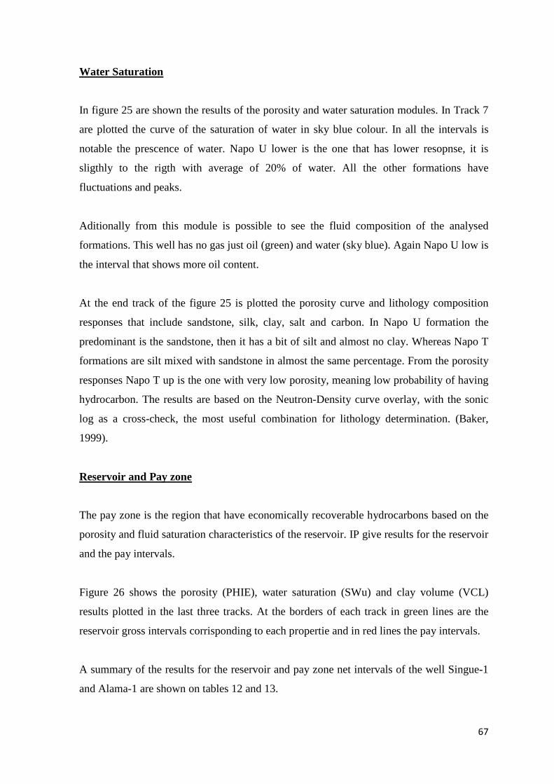
67
Water Saturation
In figure 25 are shown the results of the porosity and water saturation modules. In Track 7
are plotted the curve of the saturation of water in sky blue colour. In all the intervals is
notable the prescence of water. Napo U lower is the one that has lower resopnse, it is
sligthly to the rigth with average of 20% of water. All the other formations have
fluctuations and peaks.
Aditionally from this module is possible to see the fluid composition of the analysed
formations. This well has no gas just oil (green) and water (sky blue). Again Napo U low is
the interval that shows more oil content.
At the end track of the figure 25 is plotted the porosity curve and lithology composition
responses that include sandstone, silk, clay, salt and carbon. In Napo U formation the
predominant is the sandstone, then it has a bit of silt and almost no clay. Whereas Napo T
formations are silt mixed with sandstone in almost the same percentage. From the porosity
responses Napo T up is the one with very low porosity, meaning low probability of having
hydrocarbon. The results are based on the Neutron-Density curve overlay, with the sonic
log as a cross-check, the most useful combination for lithology determination. (Baker,
1999).
Reservoir and Pay zone
The pay zone is the region that have economically recoverable hydrocarbons based on the
porosity and fluid saturation characteristics of the reservoir. IP give results for the reservoir
and the pay intervals.
Figure 26 shows the porosity (PHIE), water saturation (SWu) and clay volume (VCL)
results plotted in the last three tracks. At the borders of each track in green lines are the
reservoir gross intervals corrisponding to each propertie and in red lines the pay intervals.
A summary of the results for the reservoir and pay zone net intervals of the well Singue-1
and Alama-1 are shown on tables 12 and 13.
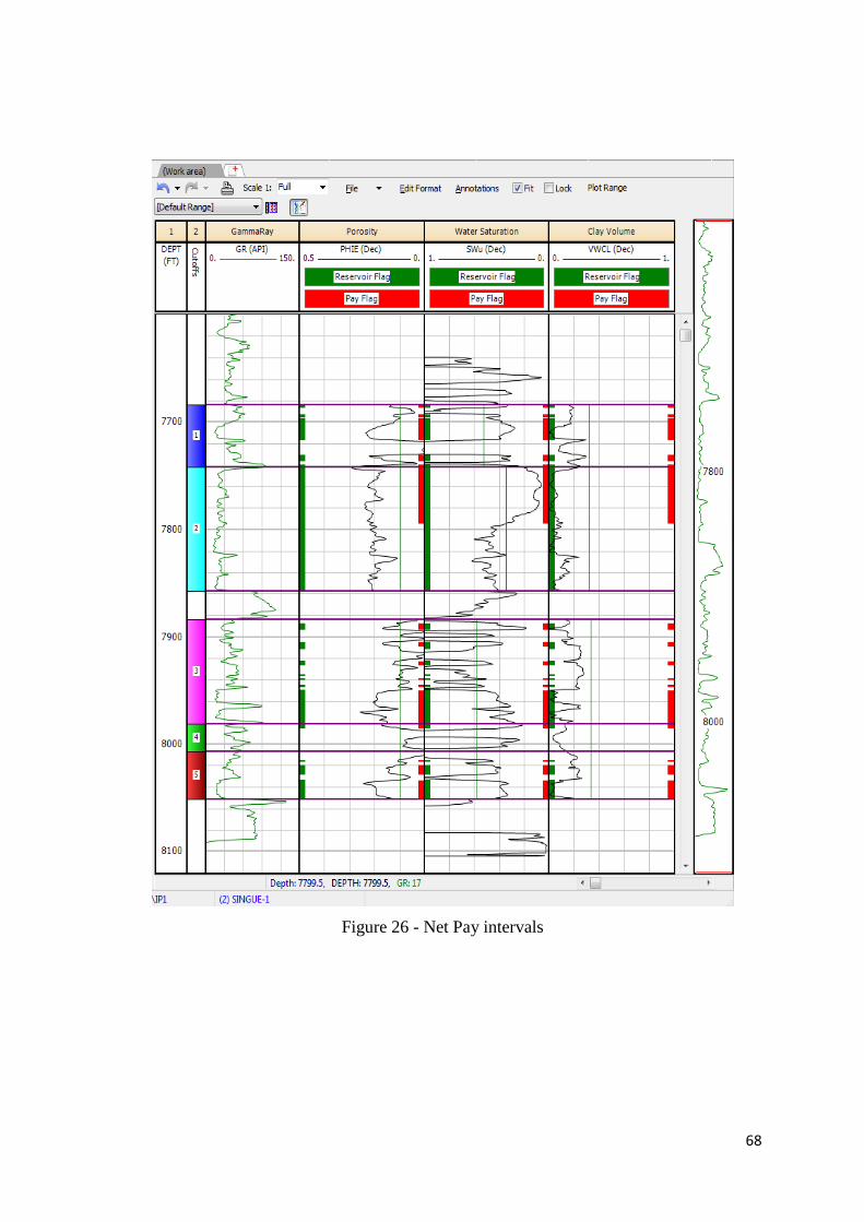
68
Figure 26 - Net Pay intervals

69
Table 12a - SINGUE petrophysical results of the reservoir interval
Table 13b - SINGUE petrophysical results of the net pay interval
Table 14a - ALAMA petrophysical results of the reservoir interval
Table 15b - ALAMA petrophysical results of the net pay interval

70
Singue-1 Net Pay interval of the Napo U low formation is the one with higher average
porosity results (21%) and less water saturation (14%), therefore this information support
previous results, concluding this formation is the better to produce oil in the field. On the
other hand, Napo T up is the one with less porosity (16%) and high water saturation (39%),
meaning cannot be a potential productive formation.
The other facies have values that are going to be computed to have an idea of the potential,
but are not as explicit as Napo U low. Napo T low has porosity of 15% and Sw of 26%,
that means could be the second important formation followed by Napo U up that has
porosity of 17% and Sw of 35%. Napo Basal has porosity of 17% and Sw of 39%.
The results of the well Alama-1 on the pay interval show that the thickness is less than in
Singue-1 for all facies. Additionally all the intervals have high water saturation with values
above 33%. Porosity results in this well are not so different to Singue-1 results. With this
information could be concluded that the lithology could be the same for both wells, but
Alama-1 might be in a different structure that is water saturated even for the Napo U low
facie compared to Singue-1 that shows good probabilities of oil in the Napo low litho-
facie.
Since Singue-1 is the well that has historical production data and that Alama was dry well,
values of the Net Pay interval of Singue-1 are going to be used for the reserves estimation
(Table 12b).
5.2 SEISMIC INTERPRETATION
Next step was the seismic interpretation of the seismic data in Petrel. To define the area of
possible hydrocarbon accumulation 20 seismic lines distributed along 150 km that cover an
area of 170 km2 were used to define the boundaries of the reservoir.
Figure 27 show the distribution of the seismic lines in 2D and 3D views. The first step was
the well tie process.

71
Figure 27 - Seismic interpretation
WELL TIE 5.2.1
With the picked well tops and after the well correlation the purpose is to locate the
information in the seismic sections, for those reason the well tie process to generate a
synthetic seismogram was done using the tops and the sonic logs. Synthetic seismograms
are used to identify the well tops in time scale and then relate it with the seismic surveys.
Then any changes from time-depth relationship can be made and seismic horizons can be
correlated with the stratigraphic boundaries identified in the well logs. (Schlumberger,
2011).
The input for the process is the sonic/density log and the seismic line where is located the
well. Sonic logs give a very detailed picture of the variation in velocity along the borehole;
however they must be integrated to give a depth time relationship. (Schlumberger, 2011)
Figure 28 shows the well tie process results. From the left side to the right the tracks of the
figure are described. The first two are the time and depth scales. Then is the sonic/density
log that was input to the process. The next track is used for the GR as a reference of
lithology. Well tops are defined by red lines.

72
On the right side of the figure are the seismic lines on both sides of the synthetic. Blue and
red colours show the reflection waves polarity of both seismic surveys and synthetic. It is
easy to follow colours at the moment of the interpretation. As it is shown in figure 28, the
synthetic wave responses are very accurate and match with the seismic data. However, the
resolution is decreasing in deeper intervals.
Figure 28 - Well Tie
Table 16 – Well tops

73
The well tie process was done manual based on the display plots, following the reflection
waves. As result of the process the well tops now have a value in time that was
automatically generated. Table 14 shows the well tops originally in depth (Z) now with the
equivalent time value (TWT).
HORIZON INTERPRETATION 5.2.2
Seismic sections show the response of the earth to seismic waves. When there are changes
in rock character in bed boundaries, wiggles occur. There is a coincidence of wiggle types
at about the same travel times. The areas of agreement are known as “seismic horizons”.
Petrel put colour to the lines of wave agreement to make interpretation easier for the
geologist or geophysicist.
Mapping started in the location of the well tops. The first trace belonged to the Top Napo
U up formation that is a well-defined reflection line that was used as reference for the work
to identify deeper reflectors. Then the other lithofacies were mapped matching the seismic
lines with the well tops.
The interpretation was done originally in the line CP-326E. After several reflector horizons
were traced across the first section then it was done along the vertical intersection lines
CP-119 and CP-128. Then with the marks projected as reference interpretation, next
sections were interpreted to match the interpreted horizons throughout the area of
coverage.
On figure 29 is explained the horizon interpretation process. On the left window is the
overview of the area and the available 2D seismic sections. In the middle window is the 3D
view of the area. At the right is the interpretation window. With yellow colour is defined
the current line that has been interpreted. With different colours are defined the picked
horizons. The X marks show the horizon cross sections picked with the same colour in
other seismic surveys.
The interpreted horizons are in the range of 1600 to 1700 TWT (two way time). Definition
of the lines is decreased on the deeper horizons which made difficult the interpretation in
all the area.
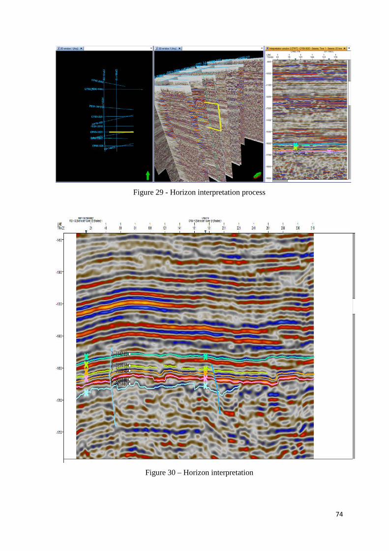
74
Figure 29 - Horizon interpretation process
Figure 30 – Horizon interpretation

75
It was concluded the existence of a slightly anticline in the area of the well Singue-1 along
the direction north – south. The interpreted section has east-west direction and shows
structural closure at different levels, which means there might be a hydrocarbon trap
capable of petroleum storage. Figure 30 show one of the interpretation windows.
FAULT INTERPRETATION 5.2.3
Fault interpretation was made creating a line starting line CP-326E on the area where the
horizons presented discontinuity. Manually lines were traced in the area of the horizon
discontinuity. Two main faults were found on the first 2D line, and then they were
projected to the other 2D sections of the area.
At the west side of the structure there is a fault, apparently is on the west border of the
structure. At the east side is another fault that do not is in contact with the structure and
that separates the wells Alama-1 and Singue-1.
The faults were found in the region close to the area of the well Singue -1. Those faults are
consistent in the shallow regions, but in the lines that are deeper those faults are not clear
defined. Could be concluded that the faults are north south orientated.
Figure 31 - Fault interpreatation

76
Figure 31 show interpretation window for the fault interpretation. In blue is defined the
fault at the east side of the field. In green is the fault that is at the west side of the field. In
between the two faults is the well Singue-1 in yellow. The well Alama-1 is on green
clearly out the area of Singue-1. These results ascertain that the two wells are not in the
same structure.
RESERVOIR BOUNDARY 5.2.4
To find the boundary of the reservoir the interpreted horizons and faults were required.
After processing the information in Petrel was possible to create surfaces of each horizon
with interpolation algorithms. Then, it was possible to create maps of each surface in
which the structure contour of each formation could be identified.
Figure 32 - Singue boundary
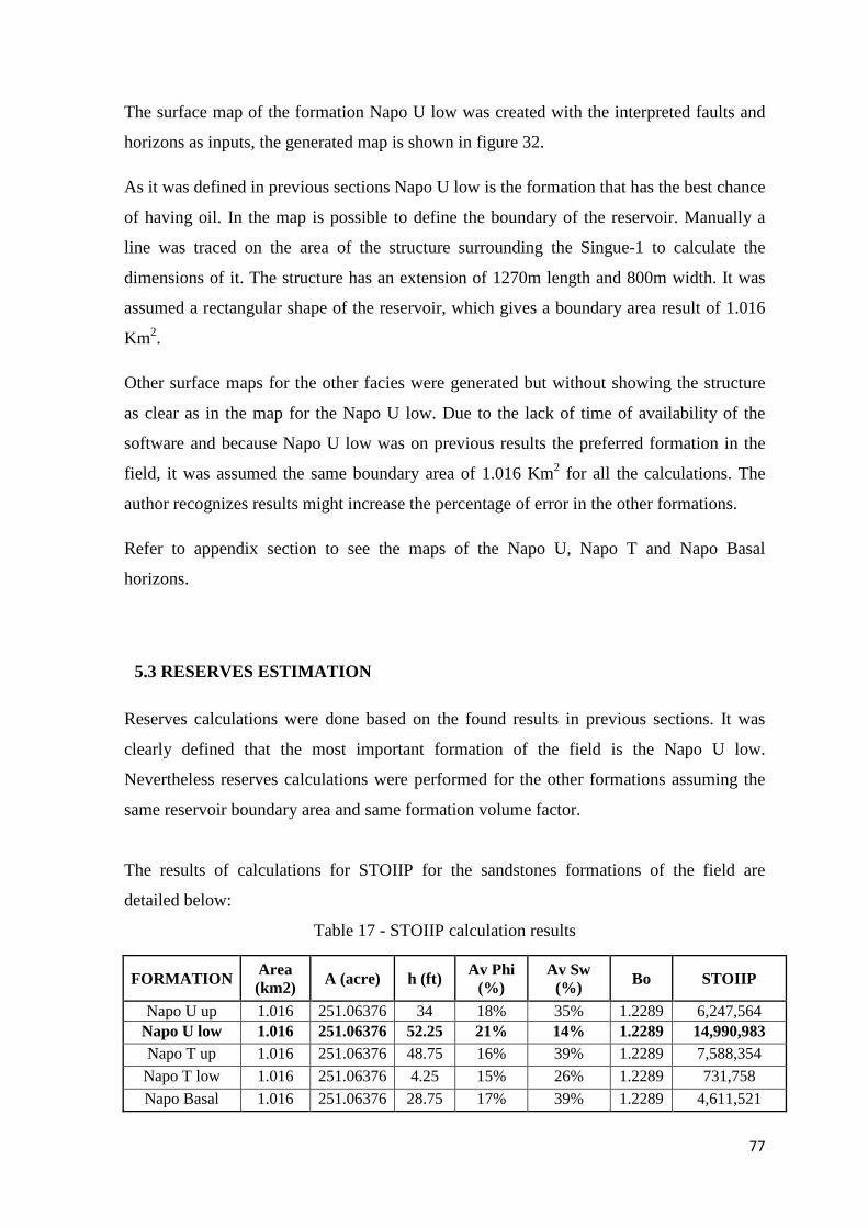
77
The surface map of the formation Napo U low was created with the interpreted faults and
horizons as inputs, the generated map is shown in figure 32.
As it was defined in previous sections Napo U low is the formation that has the best chance
of having oil. In the map is possible to define the boundary of the reservoir. Manually a
line was traced on the area of the structure surrounding the Singue-1 to calculate the
dimensions of it. The structure has an extension of 1270m length and 800m width. It was
assumed a rectangular shape of the reservoir, which gives a boundary area result of 1.016
Km2.
Other surface maps for the other facies were generated but without showing the structure
as clear as in the map for the Napo U low. Due to the lack of time of availability of the
software and because Napo U low was on previous results the preferred formation in the
field, it was assumed the same boundary area of 1.016 Km2 for all the calculations. The
author recognizes results might increase the percentage of error in the other formations.
Refer to appendix section to see the maps of the Napo U, Napo T and Napo Basal
horizons.
5.3 RESERVES ESTIMATION
Reserves calculations were done based on the found results in previous sections. It was
clearly defined that the most important formation of the field is the Napo U low.
Nevertheless reserves calculations were performed for the other formations assuming the
same reservoir boundary area and same formation volume factor.
The results of calculations for STOIIP for the sandstones formations of the field are
detailed below:
Table 17 - STOIIP calculation results
FORMATION Area (km2) A (acre) h (ft) Av Phi
(%) Av Sw
(%) Bo STOIIP
Napo U up 1.016 251.06376 34 18% 35% 1.2289 6,247,564 Napo U low 1.016 251.06376 52.25 21% 14% 1.2289 14,990,983 Napo T up 1.016 251.06376 48.75 16% 39% 1.2289 7,588,354 Napo T low 1.016 251.06376 4.25 15% 26% 1.2289 731,758 Napo Basal 1.016 251.06376 28.75 17% 39% 1.2289 4,611,521

78
Napo U low is the formation with highest STOIIP. It was the formation that the well
Singue-1 was producing in the past and is the one with higher potential.
For the reserves calculations was assumed a recovery factor of 25%, value that is common
in sandstone oil/water reservoirs of the area.
Calculation results for initial and remaining reserves in the field are detailed below:
Table 18 - Reserves calculation results
FORMATION STOIIP RF INITIAL RESERVES (bbl)
PRODUCTION (bbl)
REMAINIG RESERVES (bbl)
Napo U up 6,247,564.42 0.25 1,561,891 0 1,561,891 Napo U low 14,990,983.12 0.25 3,747,746 477000 3,270,746 Napo T up 7,588,354.14 0.25 1,897,089 0 1,897,089
Napo T low 731,758.82 0.25 182,940 0 182,940 Napo Basal 4,611,521.14 0.25 1,152,880 0 1,152,880
TOTAL 8,065,545
Figure 33 - Remaining Reserves Distribution
19%
41%
24%
2%
14%
Reserves Estimation
Napo U up
Napo U low
Napo T up
Napo T low
Napo Basal

79
As is shown on figure 33 and from the obtained results it is concluded that the field has one
important formation that is Napo U low with a recoverable reserve volume of 3.2 MMbls,
which represent the 41% of the total amount of recoverable calculated oil.
There are two other formation with high potential of having petroleum, those are: Napo T
up, Napo U up and Napo Basal T with the 24%, 19% and 14% of oil reserves as is shown
in figure 33. The total reserves for the main 4 formations reach around 7.8 MM of barrels.
The volume calculated corresponds to a marginal field in Ecuador, which represent a field
with less the 1% of production of the nation. The next step is to continue with the
modelling of the reservoir to have the water oil contact and property maps of each
formation. If it is possible to get data of one extra well in the area, a 3D model could be
created to assess in the decisions about the field. The economical evaluation of the project
to develop more wells or to put in production the ones that are there, with the option of
new formations must be done in order to evaluate the opportunity of investment.

80
6. CONCLUSIONS AND RECOMMENDATIONS
6.1 CONCLUSIONS
Exploration is one of the most important stages in the oil industry. Seismic interpretation
and well logging analysis could be used together to calculate the reserves. Specialized
software like the used in this project: Interactive Petrophysics and Petrel, help to get faster
and accurate results. As long as more information of more wells become available an
accurate results could be achieved. At beginning stages or when not too many data is
available for a field it is a challenge for petroleum engineers to assess in this kind of
projects. Experience and collaboration with professionals of areas such as Geology,
Geophysics, Petrophysics and Reservoir Engineering is recommended.
The field Singue belongs to the Oriente Basin and has a main oil productive formation
which is Napo. The sandstones facies of Napo with high oil potential production are the
Napo U low, Napo U up, Napo T up and Napo Basal. Napo U low is the one with highest
petroleum potential. Oil remaining reserves in Napo U low reach a volume of 3.2 MMbbls.
The reserves taking into account the other three important formations reach 7.8 MMbbls.
The interpreted section has east-west direction and shows structural closure at different
levels giving the possibility of being hydrocarbon traps. The structure is demonstrated as
an anticlinal extended in direction north-south . Two faults divide the wells Singue-1 and
Alama-1.
The development of marginal fields such as the one of the present case of study is
becoming necessary in countries as Ecuador that is an oil producer developing country.
Even if the amount of oil is not bigger compared with other fields, it is an attractive
opportunity of business for any petroleum company. In addition because of the world
energy demand is increasing, thus the consumption of oil is increasing and the reserves
decreasing and the need of development of new technologies and small fields is important
to satisfy that demand.
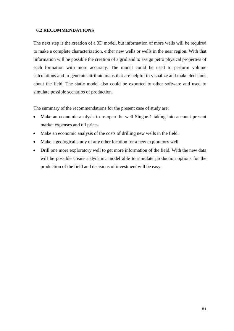
81
6.2 RECOMMENDATIONS
The next step is the creation of a 3D model, but information of more wells will be required
to make a complete characterization, either new wells or wells in the near region. With that
information will be possible the creation of a grid and to assign petro physical properties of
each formation with more accuracy. The model could be used to perform volume
calculations and to generate attribute maps that are helpful to visualize and make decisions
about the field. The static model also could be exported to other software and used to
simulate possible scenarios of production.
The summary of the recommendations for the present case of study are:
• Make an economic analysis to re-open the well Singue-1 taking into account present
market expenses and oil prices.
• Make an economic analysis of the costs of drilling new wells in the field.
• Make a geological study of any other location for a new exploratory well.
• Drill one more exploratory well to get more information of the field. With the new data
will be possible create a dynamic model able to simulate production options for the
production of the field and decisions of investment will be easy.
82
7. REFERENCES AND BIBLIOGRAPHY
Asquith, G. a. (2004). Basic well log analysis. American Association of Petroleum
Geologists, 244.
Baby P, R. M. (2004). La Cuenca oriente: geología y petróleo. Quito: ”, Andean studies
French Institute, Institut de Recherche pour le Développement, Petroecuador.
Bacon, M. M. (2003). 3-D Seismic Interpretation. Cambridge University Press.
Cambridge.
Baldock. (1982). “Geología del Ecuador”. Explanation of Ecuadorean geological map
bulletin Scale 1:1000.000, 66.
Boggs, A. (2001). Principles of sedimentary stratigraphy.
Bradley. (1985). In K. D., Tectonic Growth of a collisional continental margin: Crustal
evolution of Southern Alaska (p. 72). Geological Society of America.
CGG. (n.d.). CGG Passion for geoscience. Retrieved 04 03, 2014, from
http://www.cgg.com
Connolly, E. (1965). Production logging, a resume and current status of the use of logs in
production, Correlation of different maturity parameters in the Ahmed Abad-
Mehsana block of the Cambay Basin. SPWLA Symposium: Organic Geochemistry.
Dallas. .
Conversion units. (n.d.). Retrieved from
http://home.hiwaay.net/~taylorc/toolbox/geography/geoutm.html,
http://transition.fcc.gov/mb/audio/bickel/DDDMMSS-decimal.html
Darling, T. (2005). Well logging and formation evaluation. Boston: Elsevier.
Dashwood M F, A. I. (1990). Aspects of the petroleum geology of the Oriente Basin, .
Ecuador Geologic Society Special Publications, 89–117.
Etherington J., P. T. (2005). Comparison of Selected Reserve, Resource Classifications and
Associated Definitions. SPE Oil and Gas Reserves Committee (OGRC).

83
Faytteville Shale Natural Gas. (n.d.). Searching for natural gas. Retrieved 04 03, 2014,
from http://lingo.cast.uark.edu/LINGOPUBLIC/antgas/search/index.htm
Granja, J. C. (1976). El Petróleo misceláneas. Quito: Universitaria Editorial. .
J. Estupiñan, R. M. (2010). Reservoir sandstones of the cretaceous Napo formation U and
T members in the Oriente basin, Ecuador: links between diagenesis and sequence
stratigraphy. Journal of Petroleum Geology Vol. 33.
J. Estupiñan, R. M. (n.d.). Reservoir sandstones of the cretaceous napo formation u and t
members in the oriente basin, ecuador: links between diagenesis and sequence
stratigraphy. Journal of Petroleum Geology V. 33, 221-246.
Ltd., S. S. (2011). Interactive Petrophysics 4.0 Help document .
M., J. (2008). Hydrocarbon Exploration and Production. Amsterdam: Elsevier.
Marocco R, L. A. (1995). Intermontane Late Paleogene-Neogene Basins of the Andes of
Ecuador and Peru, sedimentologic and tectonic characteristics. In S. S. In: Tankard
A, Petroleum basins of South America.
Murtha J., R. J. (2009). Uncertainty and the Volumetric Equation. . JPT.
Myers, G. (2007). Nuclear Logging, Reservoir Engineering and Petrophysics Volume
V(A). In Petroleum Engineering Handbook (pp. V-267 to V-287). Edward
Holstein, Editor.
Petroecuador. (2010). El petroleo en el Ecuador.
Petroproduccion. (1990). Geophysic prospect of Singue.
Petroproduccion. (1991). Biostratigraphic and Paleologic report of the well Singue-1.
Ordonez M., Zambrano I., Jimenez N.
Petroproduccion. (1991). Core sample analysis.
Petroproduccion. (1994). PVT Analysis, Singue-1, Lower U sandstone. .
PGE, N. D. (2013). Hydrocarbons Law, Ecuador.
84
Pindell J L, T. K. (1995). Mesozoic-Cenozoic Andean paleogeography and regional
controls on hydrocarbon systems. In S. S. Tankard A, Petroleum basins of South
America (pp. 101-128). Tulsa.
Rivadeneira M, B. P. (2004). La cuenca oriente: Geologia y petroleo. Quito: Andean
studies French Institute - Petroecuador.
Russell, W. (1944). The total gamma ray activity of sedimentary rocks as indicated by
Geiger counter determinations. Geophysics 9 (2), pp. 180-226.
San Joaquin Valley Geology. (n.d.). Well logs. Retrieved 04 05, 2014, from
http://www.sjvgeology.org/oil/logs.html
Schlumberger. (2010). Petrel 2010: Seismic visualization and interpretation. .
Schlumberger. (2011). Petrel Help manual.
Schlumberger. (2014). Petrel E&P Software plataform. Retrieved 04 01, 2014, from
Schlumberger Software:
http://www.software.slb.com/products/platform/Pages/petrel.aspx
Selley, C. (1998). Elements of Petroleum Geology. San Diego, California: Academic Press.
Selley, R. (1998). Elements of Petroleum Geology. . Academic Press. Second Edition.
Senergy. (2014). Interactive Petrophysics webpage. Retrieved 04 28, 2014, from Senergy
World: http://www.senergyworld.com/software/interactive-petrophysics
Senergy Software Ltd. (2011). Interactive Petrophysics 4.0 Help document (2011).
SHC. (2011). Decima ronda petrolera. Retrieved 02 11, 2014, from Secretary of
Hydrocarbons Ecuador: http://www.shc.gob.ec/portal/web/ronda-
petrolera/documentacion-singue
SPE. (2013, 07 19). Petrowiki. Retrieved 04 07, 2014, from Resistivity and SP logging:
http://petrowiki.org/Resistivity_and_spontaneous_(SP)_logging
Tarek H. (2004). Advanced reservoir engineering. Oxford: Gulf Professional.
85
Valasek D, A. A. (1996). Cretaceous sequence stratigraphy of the Maranon-Oriente-
Putumayo Basins, northeastern Peru, eastern Ecuador, and Southeastern Colombia.
. AAPG Bulletin, 80(8): 1341–1342.
Vali, P., Mitchum, R., & Thompson, S. (1977). Seismic stratigraphy and global changes of
sea level.
Wasserstrom, R. R. (2013). Corporate responsability and Oil in Ecuador and Nigeria.
Anthropologists, 77-91.
Weber, K., & Van Genus, L. (1990). Framework for constructiong clastic reservoir
simulation models. Journal of Petroleum Technology.
White, H. S. (1995). Reservoir characteristics of Hollín and Napo Formations, western
Oriente basin, Ecuador. In Petroleum basin of South America. (pp. AAPG Memoir,
62, 573–596.).
Xie Yinfu, J. S. (2010). Petroleum geology and exploration potential of Oriente-Maranon
Basin (Vol. 37 (1)). PETROL. EXPLOR. DEVELOP.

86
APPENDIX
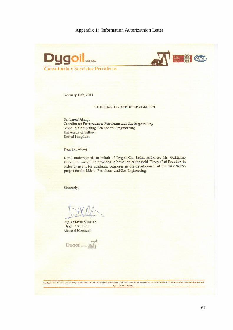
87
Appendix 1: Information Autorizathion Letter

-1637.5
-1637.5
-1637.5
-1637.5
-1625
-1612.5
-1637.5-1
637.5
-1637.5
-1637.5
Alama-1
Singue-1
356000 356800 357600 358400 359200 360000 360800
356000 356800 357600 358400 359200 360000 360800
1.00
17E
+7
1.00
18E
+7
1.00
19E
+7
1.00
2E+
71.
0021
E+
71.
0022
E+
71.0017E
+7
1.0018E+
71.0019E
+7
1.002E+
71.0021E
+7
1.0022E+
7
0 500 1000 1500 2000 2500m
1:40000
-1650-1647.5-1645-1642.5-1640-1637.5-1635-1632.5-1630-1627.5-1625-1622.5-1620-1617.5-1615-1612.5-1610-1607.5
Elevation time [ms]
Symbol legendOil Undefined
Country
Block
License
Model name
Horizon name
Scale
Contour inc
User name
Date
Signature
1:40000
2.5
stp782
05/27/2014
Map
Top Napo U

-1660 -1665
-1665
-167
0
-1665
-1660
-1660
-1655
-1660
-1660
-166
5
-166
5
-1655
-1660
-1660-1660
-1665
-1665
-1670
-1670
Alama-1
Singue-1
356000 356500 357000 357500 358000 358500 359000 359500 360000
356000 356500 357000 357500 358000 358500 359000 359500 360000
1.00
168E
+7
1.00
176E
+7
1.00
184E
+7
1.00
192E
+7
1.00
2E+
71.
0020
8E+
71.00168E
+7
1.00176E+
71.00184E
+7
1.00192E+
71.002E
+7
1.00208E+
7
0 250 500 750 1000 1250m
1:32000
-1677-1676-1675-1674-1673-1672-1671-1670-1669-1668-1667-1666-1665-1664-1663-1662-1661-1660-1659-1658-1657-1656-1655-1654-1653-1652-1651
Elevation time [ms]
Symbol legendOil Undefined
Top Napo T
Country
Block
License
Model name
Horizon name
Scale
Contour inc
User name
Date
Signature
1:32000
1
stp782
05/27/2014
Map

-168
0
-1670
-1670
-1670 -1670
-1670
-1680
-1680
-1680
-1670
-1670
-1670
-1660
-1670
-1680 -1
690
-1680
-1680
-1680
Alama-1
Singue-1
356000 356800 357600 358400 359200 360000 360800
356000 356800 357600 358400 359200 360000 360800
1.00
16E
+7
1.00
17E
+7
1.00
18E
+7
1.00
19E
+7
1.00
2E+
71.
0021
E+
71.
0022
E+
71.0016E
+7
1.0017E+
71.0018E
+7
1.0019E+
71.002E
+7
1.0021E+
71.0022E
+7
0 500 1000 1500 2000 2500m
1:40000
-1690-1688-1686-1684-1682-1680-1678-1676-1674-1672-1670-1668-1666-1664-1662-1660-1658-1656-1654
Elevation time [ms]
Country
Block
License
Model name
Horizon name
Scale
Contour inc
User name
Date
Signature
1:40000
2
stp782
05/27/2014
Map
Top Napo Basal