Equilibria in Heterogeneous Nonmonotonic Multi-Context Systems

Gerhard BrewkaDept. of Computer Science

University of LeipzigJohannisgasse 26, D-04103 Leipzigbrewka@informatik.uni-leipzig.de

Thomas EiterInstitute of Information SystemsVienna University of Technology

Favoritenstrasse 11, A-1040 Viennaeiter@kr.tuwien.ac.at

Abstract

We propose a general framework for multi-context reasoningwhich allows us to combine arbitrary monotonic and non-monotonic logics. Nonmonotonic bridge rules are used tospecify the information flow among contexts. We investigateseveral notions of equilibrium representing acceptable beliefstates for our multi-context systems. The approach general-izes the heterogeneous monotonic multi-context systems de-veloped by F. Giunchiglia and colleagues as well as the ho-mogeneous nonmonotonic multi-context systems of Brewka,Serafini and Roelofsen.

Background and Motivation

Interest in formalizations of contextual information andinter-contextual information flow has steadily increased overthe last years. Based on seminal papers by McCarthy (1987)and Giunchiglia (1993), several approaches have been pro-posed, most notably McCarthy’s propositional logic of con-text (1993) and the multi-context systems of the Trentoschool devised by Giunchiglia and Serafini (1994).

Intuitively, a multi-context system describes the informa-tion available in a number of contexts (i.e., to a number ofpeople/agents/databases/modules, etc.) and specifies the in-formation flow between those contexts. The contexts them-selves may be heterogeneous in the sense that they can usedifferent logical languages and different inference systems,and no notion of global consistency is required. The infor-mation flow is modeled via so-called bridge rules which canrefer in their premises to information from other contexts.

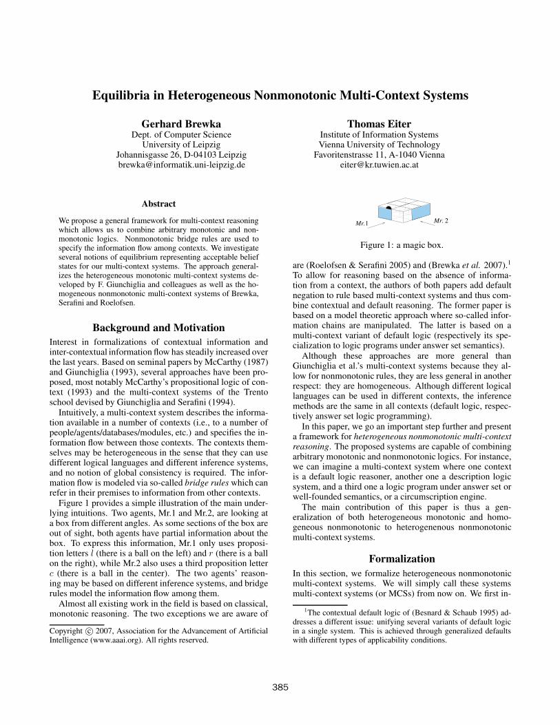
Figure 1 provides a simple illustration of the main under-lying intuitions. Two agents, Mr.1 and Mr.2, are looking ata box from different angles. As some sections of the box areout of sight, both agents have partial information about thebox. To express this information, Mr.1 only uses proposi-tion letters l (there is a ball on the left) and r (there is a ballon the right), while Mr.2 also uses a third proposition letterc (there is a ball in the center). The two agents’ reason-ing may be based on different inference systems, and bridgerules model the information flow among them.

Almost all existing work in the field is based on classical,monotonic reasoning. The two exceptions we are aware of

Copyright c© 2007, Association for the Advancement of ArtificialIntelligence (www.aaai.org). All rights reserved.

Mr.1 Mr. 2

Figure 1: a magic box.

are (Roelofsen & Serafini 2005) and (Brewka et al. 2007).1

To allow for reasoning based on the absence of informa-tion from a context, the authors of both papers add defaultnegation to rule based multi-context systems and thus com-bine contextual and default reasoning. The former paper isbased on a model theoretic approach where so-called infor-mation chains are manipulated. The latter is based on amulti-context variant of default logic (respectively its spe-cialization to logic programs under answer set semantics).

Although these approaches are more general thanGiunchiglia et al.’s multi-context systems because they al-low for nonmonotonic rules, they are less general in anotherrespect: they are homogeneous. Although different logicallanguages can be used in different contexts, the inferencemethods are the same in all contexts (default logic, respec-tively answer set logic programming).

In this paper, we go an important step further and presenta framework for heterogeneous nonmonotonic multi-contextreasoning. The proposed systems are capable of combiningarbitrary monotonic and nonmonotonic logics. For instance,we can imagine a multi-context system where one contextis a default logic reasoner, another one a description logicsystem, and a third one a logic program under answer set orwell-founded semantics, or a circumscription engine.

The main contribution of this paper is thus a gen-eralization of both heterogeneous monotonic and homo-geneous nonmonotonic to heterogenenous nonmonotonicmulti-context systems.

Formalization

In this section, we formalize heterogeneous nonmonotonicmulti-context systems. We will simply call these systemsmulti-context systems (or MCSs) from now on. We first in-

1The contextual default logic of (Besnard & Schaub 1995) ad-dresses a different issue: unifying several variants of default logicin a single system. This is achieved through generalized defaultswith different types of applicability conditions.

385

troduce MCSs, and then define several notions of equilibriafor them. An equilibrium is a collection of belief sets foreach context such that each belief set is based on the knowl-edge base of the respective context together with the infor-mation conveyed through applicable bridge rules.

As we will see, equilibria allow for certain forms of self-justification via the bridge rules. For this reason, we discussminimal equilibria and finally grounded equilibria. The lat-ter can only be defined for the subclass of reducible MCSs.

Multi-context systems

The idea behind heterogeneous MCSs is to allow differentlogics to be used in different contexts, and to model informa-tion flow among contexts via bridge rules. We first describewhat we mean by a logic here.

We will characterize the syntax of a logic L by specifyingthe set KBL of its well-formed knowledge bases. Withoutloss of generality, we assume the knowledge bases are sets.In cases where the standard definition of a knowledge basehas more structure (like in default logic where default the-ories consist of a set of formulas and a set of defaults), wecan always make sure that elements of different substruc-tures can be distinguished syntactically.

We also need to describe L’s possible belief sets BSL,that is sets of syntactical elements representing the beliefsan agent may adopt. In most cases this will be deductivelyclosed sets of formulas, but we may have further restrictions,e.g. to sets of atoms, sets of literals, and the like.

We finally have to characterize acceptable belief sets anagent may adopt based on the knowledge represented in aknowledge base. For classical, monotonic logics this willnormally just be the set of classical consequences of theknowledge base. However, in many of the typical rule-basednonmonotonic systems multiple acceptable belief sets mayarise (called extensions, expansions, answer sets etc.). Forthis reason we will characterize acceptable belief sets usinga function ACCL assigning to each knowledge base kb a setof belief sets taken from BSL.

Definition 1 A logic L = (KBL, BSL, ACCL) is composedof the following components:

1. KBL is the set of well-formed knowledge bases of L. Weassume each element of KBL is a set.

2. BSL is the set of possible belief sets,

3. ACCL : KBL → 2BSL is a function describing the “se-mantics” of the logic by assigning to each element of KBL

a set of acceptable sets of beliefs.

Example 1 Let us first discuss some example logics, de-fined over a signature Σ:

• Default logic (DL) (Reiter 1980):

– KB: the set of default theories based on Σ,

– BS: the set of deductively closed sets of Σ-formulas,

– ACC(kb): the set of kb’s extensions.

• Normal logic programs under answer set semantics (NLP)(Gelfond & Lifschitz 1991):

– KB: the set of normal logic programs over Σ,

– BS: the set of sets of atoms over Σ,

– ACC(kb): the set of kb’s answer sets.

• Propositional logic under the closed world assumption:

– KB: the set of sets of propositional formulas over Σ,

– BS: the set of deductively closed sets of propositionalΣ-formulas,

– ACC(kb): the (singleton set containing the) set of kb’sconsequences under closed world assumption.

There are numerous other examples, nonmonotonic (e.g.,circumscription, autoepistemic logic, defeasible logic) aswell as monotonic (e.g., description logics, modal logics,temporal logics). We next define multi-context systems.

Definition 2 Let L = {L1, . . . , Ln} be a set of logics. AnLk-bridge rule over L, 1 ≤ k ≤ n, is of the form

s ← (r1 : p1), . . . , (rj : pj),not (rj+1 : pj+1), . . . , not (rm : pm)

(1)

where 1 ≤ rk ≤ n, pk is an element of some belief set ofLrk

, and for each kb ∈ KBk : kb ∪ {s} ∈ KBk.

Definition 3 A multi-context system M = (C1, . . . , Cn)consists of a collection of contexts Ci = (Li, kbi, bri),where Li = (KBi, BSi, ACCi) is a logic, kbi a knowledgebase (an element of KBi), and bri is a set of Li-bridge rulesover {L1, . . . , Ln}.

We use head(r) to denote the head of a bridge rule r.Bridge rules refer in their bodies to other contexts and canthus add information to a context based on what is be-lieved or disbelieved in other contexts. Note that in con-trast with Giunchiglia’s (monotonic) multi-context systems,in our systems there is no single, global set of bridge rules.To emphasize their locality, we add the bridge rules to thosecontexts to which they potentially add new information.

Equilibria

We now need to define the acceptable belief states a sys-tem may adopt. These belief states have to be based on theknowledge base of each context, but also on the informationcontained in other contexts in case there is an appropriate ap-plicable bridge rule. Intuitively, we have to make sure thatthe chosen belief sets are in equilibrium: for each context Ci

the selected belief set must be among the acceptable beliefsets for Ci’s knowledge base together with the heads of Ci’sapplicable bridge rules.

Definition 4 Let M = (C1, . . . , Cn) be an MCS. A beliefstate is a sequence S = (S1, . . . , Sn) such that each Si isan element of BSi.

We say a bridge rule r of form (1) is applicable in a beliefstate S = (S1, . . . , Sn) iff for 1 ≤ i ≤ j: pi ∈ Sri

and forj + 1 ≤ k ≤ m: pk �∈ Srk

.

Definition 5 A belief state S = (S1, . . . , Sn) of M is anequilibrium iff, for 1 ≤ i ≤ n, the following condition holds:

Si ∈ ACCi(kbi ∪ {head(r) | r ∈ bri applicable in S}).

An equilibrium thus is a belief state which contains for eachcontext an acceptable belief set, given the belief sets of theother contexts.2

2One can view each context as a player in an n-person gamewhere players choose belief sets. Assume for a given profile

386

Minimal equilibria

Equilibria are not necessarily minimal (under component-wise set inclusion). They allow for a certain form of self-justification of elements of belief sets via bridge rules.

Example 2 Consider M = (C1) with a single context basedon classical reasoning in propositional logic. Assume kb1 isempty and br1 consists of the bridge rule p ← (1 : p). Nowboth (Th(∅)) and (Th({p})) are equilibria. The latter issomewhat questionable as p is justified by itself.

In the example (and whenever all contexts are monotonic,see below) we can solve the problem by considering mini-mal equilibria. However, there may be situations where min-imality is unwanted, or at least not for all contexts. For in-stance, LPs with cardinality constraints (Niemela & Simons2000) use expressions of the form j{a1, . . . , ak}k to statethat the number of atoms in {a1, . . . , ak} contained in ananswer set must be between j and k. Answer sets thus maybe nonminimal.

Similarly, stable expansions in autoepistemic logic (AEL)(Moore 1985) are not necessarily minimal: the premise set{Lp → p} has two stable expansions, one in which onlyAEL tautologies are believed, and one where in addition p isbelieved. If a context in an MCS is based on a logic whoseacceptable belief sets are not necessarily minimal, restrictingthe attention to minimal equilibria may not be a good idea.

The following definition allows us to explicitly selectthose contexts for which minimality is required, and to keepother contexts fixed in the minimization:

Definition 6 Let M = (C1, . . . , Cn) be an MCS, S =(S1, . . . , Sn) an equilibrium of M , C∗ a subset of the con-texts in M . S is called C∗-minimal iff there is no equilibriumS′ = (S′

1, . . . , S′n) such that

1. S′i ⊆ Si for all contexts Ci ∈ C∗,

2. S′i ⊂ Si for some context Ci ∈ C∗,

3. S′i = Si for all contexts Ci �∈ C∗.

There are also cases where minimality is not strong enough.Several nonmonotonic systems like default logic or logicprograms under answer set semantics have a stronger notionof groundedness which cannot be captured by minimality. Inparticular, the contextual default logic approach described in(Brewka, Roelofsen, & Serafini 2007) is not a proper specialcase of the notion described here. The reason is that con-textual default logic has a stronger groundedness condition:some forms of “self-justification” are possible even in mini-mal equilibria which were not allowed in the quoted paper.

Example 3 Consider the MCS M = (C1, C2) consisting oftwo default logic contexts. Assume kb1 and kb2 are empty,and br1 consists of the single bridge rule p ← (2 : q) andbr2 of two rules q ← (1 : p) and r ← not (1 : p). Nowboth (Th({p}), Th({q})) and (Th(∅), Th({r})) are mini-mal equilibria, but only the latter is a contextual extensionin the sense of (Brewka et al. 2007). The former contains

(choice of belief sets by the players) each player’s utility is 1 if shepicks an acceptable belief set given her knowledge base and theheads of bridge rules applicable under the profile, and 0 otherwise.The Nash equilibria of this game coincide with our equilibria.

beliefs which justify themselves, but this cannot be excludedby requiring minimality.

Grounded equilibria

We now define grounded equilibria for a restricted classof so called reducible MCSs. Intuitively, an MCS is re-ducible if each component logic is either monotonic (eachkb has a single acceptable belief set which grows monoton-ically when information is added to kb), or it is one of thenonmonotonic systems like default logic or logic programswhere a candidate belief set S is tested for groundedness bytransforming the original knowledge base kb to a simplerone kb′. S is accepted if it coincides with the belief set ofkb′. The standard example is the Gelfond/Lifschitz reduc-tion for logic programs. For bridge rules we will introducea similar reduction.

Definition 7 Let L = (KBL, BSL, ACCL) be a logic. L iscalled monotonic iff

1. ACCL(kb) is a singleton set for each kb ∈ KBL, and

2. kb ⊆ kb′, ACCL(kb) = {S}, and ACCL(kb′) = {S′}implies S ⊆ S′.

Remark: an MCS can be nonmonotonic even if all involvedlogics are monotonic: its bridge rules can be nonmonotonic.

Definition 8 Let L = (KBL, BSL, ACCL) be a logic. L iscalled reducible iff

1. there is KB∗L ⊆ KBL such that the restriction of L to KB

∗L

is monotonic,

2. there is a reduction function redL : KBL × BSL → KB∗L

such that for each k ∈ KBL and S, S′ ∈ BSL:

• redL(k, S) = k whenever k ∈ KB∗L,

• redL is antimonotone in the second argument, that isredL(k, S) ⊆ redL(k, S′) whenever S′ ⊆ S,

• S ∈ ACCL(k) iff ACCL(redL(k, S)) = {S}.

The conditions for redL say the following: (a) k should notbe further reduced if it is already in the target class KB∗

L,(b) justifying the elements in a larger belief set cannot bemade easier than justifying a smaller set by using a largerreduced knowledge base, and (c) acceptability of a belief setcan actually be checked by the reduction.

Definition 9 A context C = (L, kb, br) is reducible iff

1. its logic L is reducible,

2. for all H ⊆ {head(r)|r ∈ br} and belief sets S:redL(kb ∪ H, S) = redL(kb, S) ∪ H .

An MCS is reducible if all of its contexts are. Note that acontext is reducible whenever its logic L is monotonic. Inthis case KB∗ coincides with KB and redL is identity withrespect to the first argument.

We can now define grounded equilibria. We follow ideas(and terminology) from logic programming:

Definition 10 Let M = (C1, . . . , Cn) be a reducible MCS.M is called definite iff

1. none of the bridge rules in any context contains not

2. for all i, S ∈ BSi: kbi = redi(kbi, S).

387

In a definite MCS bridge rules are monotonic, and knowl-edge bases are already in reduced form. Inference is thusmonotonic and a unique minimal equilibrium exists. Wetake this equilibrium to be the grounded equilibrium:

Definition 11 Let M = (C1, . . . , Cn) be a definite MCS.S = (S1, . . . , Sn) is the grounded equilibrium of M iff S isthe unique minimal equilibrium of M .

A more operational characterization of the grounded equi-librium of a definite MCS M = (C1, . . . , Cn) is providedby the following proposition. For 1 ≤ i ≤ n, let kb0

i = kbi

and define, for each successor ordinal α + 1,

kbα+1i = kbα

i ∪ {head(r) | r ∈ bri is applicable in Eα},

where Eα = (Eα1 , . . . , Eα

n ) and ACCi(kbαi ) = {Eα

i }. Fur-

thermore, for each limit ordinal α, define kbαi =

⋃β≤α kb

βi ,

and let kb∞i =⋃

α>0 kbαi . Then we have:

Proposition 1 Let M = (C1, . . . , Cn) be a definite MCS. Abelief state S = (S1, . . . , Sn) is the grounded equilibriumof M iff ACCi(kb∞i ) = {Si}, for 1 ≤ i ≤ n.

Remark: For many logics (in particular, those satisfyingcompactness), kb∞i = kbω

i holds; that is, any bridge rule isapplied (if at all) after finitely many steps; this is also trivialif bri is finite. However, there are logics conceivable whichrequire a transfinite number of steps.

The grounded equilibrium of a definite MCS M will bedenoted GE(M). Grounded equilibria for general MCSsare defined based on a reduct which generalizes the Gel-fond/Lifschitz reduct to the multi-context case:

Definition 12 Let M = (C1, . . . , Cn) be a reducible MCS,S = (S1, . . . , Sn) a belief state of M . The S-reduct of M is

MS = (CS1 , . . . , CS

n )

where for each Ci = (Li, kbi, bri) we define CSi = (Li,

redi(kbi, Si), brSi ). Here brS

i results from bri by deleting

1. every rule with some not (k:p) in the body such that p ∈Sk, and

2. all not literals from the bodies of remaining rules.

For each MCS M and each belief set S, we have that MS isdefinite. We can thus check whether S is a grounded equi-librium in the usual manner:

Definition 13 Let M = (C1, . . . , Cn) be a reducible MCS,S = (S1, . . . , Sn) a belief state of M . S is a groundedequilibrium of M iff S is the grounded equilibrium of MS ,that is S = GE(MS).

We have the following result:

Proposition 2 Every grounded equilibrium of a reducibleMCS M is a minimal equilibrium of M .

Examples of reducible nonmonotonic systems are defaultlogic, NLPs, and LPs with cardinality constraints. For Re-iter’s default logic the reduction function red(Δ, S) takes adefault theory Δ and eliminates all defaults with justificationp such that ¬p ∈ S, and deletes all justifications from theremaining defaults. The resulting justification-free defaulttheories are monotonic and satisfy the required conditions.

Example 4 Consider again MCS M = (C1, C2) of Exam-ple 3. We saw earlier that among the two minimal equilibriaE1 = (Th({p}), Th({q})) and E2 = (Th(∅), Th({r}))only the second one has no self-justified beliefs. It is easy toverify that GE(ME1) = (Th(∅), Th(∅)) �= E1. Thus E1 isnot a grounded equilibrium, as intended. On the other hand,GE(ME2) = (Th(∅), Th({r})) = E2, and thus E2 is thesingle grounded extension of M .

Both the multi-context systems by Giunchiglia & Serafini(1994) and contextual default logic by Brewka et al. (2007)are special cases of MCSs: the former have monotonic con-texts, the latter use default logic in all contexts.

Well-founded Semantics

We can define a well-founded semantics for a reducibleMCS M based on the operator γM (S) = GE(MS), pro-vided BSi for each logic Li in any of M ’s contexts has aleast element S∗. We call MCSs satisfying this conditionnormal. The following result is a consequence of the anti-monotony of redi:

Proposition 3 Let M = (C1, . . . , Cn) be a reducible MCS.Then γM is antimonotone.

We thus obtain a monotone operator by applying γM twice.Similar to what is done in logic programming we define thewell-founded semantics of M as the least fixpoint of (γM )2.This fixpoint exists according to the Knaster-Tarski theorem.

Definition 14 Let M = (C1, . . . , Cn) be a normal re-ducible MCS. The well-founded semantics of M , denotedWFS(M), is the least fixpoint of (γM )2.

The fixpoint can be computed by iterating (γM )2 startingwith the least belief state S� = (S�

1 , . . . , S�n). The grounded

extensions of M and WFS(M) are related as usual:

Proposition 4 Let M = (C1, . . . , Cn) be a normal re-ducible multi-context system such that WFS(M) = (W1,. . . , Wn). Let S = (S1, . . . , Sn) be a grounded equilibriumof M . Then Wi ⊆ Si for 1 ≤ i ≤ n.

The well-founded semantics can thus be viewed as an ap-proximation of the belief state representing what is acceptedin all grounded equilibria. Note that WFS(M) itself is notnecessarily an equilibrium.

WFS as defined here still suffers from a weakness dis-cussed by (Brewka & Gottlob 1997) and (Brewka, Roelof-sen, & Serafini 2007). Assume γM (S�) = (T1, . . . , Tn)and one of the belief sets Ti is inconsistent and deductivelyclosed. Then none of M ’s bridge rules referring to contextCi through a body literal not (i : p) (for arbitrary p) will beused in the computation of (γM )2(S�). This may lead tooverly cautious reasoning. As discussed in the quoted pa-pers, this problem can be dealt with by considering modifiedoperators, producing sets of formulas which are not deduc-tively closed. Similar techniques can be used for MCSs.

Computational Complexity

In this section, we consider complexity aspects of MCSs.We focus on the problem of deciding whether an MCSM = (C1, . . . , Cn) has an equilibrium, and on brave (resp.,

388

cautious) reasoning from its equilibria, i.e., given an elementp, and some Ci, is p ∈ Si for some (resp., each) equilibriumS = (S1, . . . , Sn) of M . We assume familiarity with the ba-sics of complexity (see (Papadimitriou 1994)), in particularthe polynomial hierarchy (Σp

0 = Πp0 = Δp

0 = P , and, for all

k ≥ 0, Σpk+1 = NPΣ

p

k , Πpk+1 = co-Σp

k+1, and Δpk+1 = PΣ

p

k ;

here (N)PC is (non)deterministic polynomial time with anoracle for C, and co-C is the complement of class C).

Let us say that a logic L has poly-size kernels, if thereis a mapping κ which assigns to every kb ∈ KB and S ∈ACC(kb) a set κ(kb, S) ⊆ S of size (written as a string)polynomial in the size of kb, called the kernel of S, such thatthere is a one-to-one correspondence f between the beliefsets in ACC(kb) and their kernels, i.e., S � f(κ(kb, S)).Standard propositional non-monotonic logics like DL, AEL,NLP, etc. all have poly-size kernels.

If furthermore, given any knowledge base kb, an ele-ment b, and a set of elements K , deciding whether (i)K = κ(kb, S) for some S ∈ ACC(kb) and (ii) b ∈ S isin Δp

k, then we say that L has kernel reasoning in Δpk.

Note that the standard propositional NMR formalisms DLand AEL have kernel reasoning in Δp

2, and under suitablerestrictions even in Δp

1 = P, i.e., in polynomial time.

For convenience, we assume that any belief set S in anylogic L contains a distinguished element true; so for b =true, (i) and (ii) together are equivalent to (i), i.e., whetherK is a kernel for some acceptable belief set of kb.

We concentrate on finite MCS, where all knowledge baseskbi and sets of bridge rules bri are finite; the Li are from anarbitrary but fixed set. The following result gives an upperbound on deciding the existence of an equilibrium.

Theorem 1 Given a finite MCS M = (C1, . . . , Cn) whereall logics Li have poly-size kernels and kernel reasoning inΔp

k, deciding whether M has an equilibrium is in Σpk+1.

In particular, for an MCS in which the components areknowledge bases in an NMR formalism like propositionalDL, AEL, NLP, etc. deciding the existence of an equilib-rium is in the worst case not more complex than deciding theexistence of an acceptable belief set in the component log-ics. This property, however, is not automatically inherited byall fragments of a logic, because the bridge rules might addcomplexity (e.g., if all logics are propositional Horn logicprograms, but the bridge rules are unstratified).

Informally, Theorem 1 holds since we can guess kernelsκ1, . . . , κn of the belief sets S1, . . . , Sn in an equilibrium Sfor M , together with the sets of heads H1, . . . , Hn of bridgerules that are applicable in S, and check that each κi is thekernel of some Si ∈ ACC(kbi ∪ Hi), and that Hi is cor-rect; by hypothesis, checking is in Δp

k . On the other hand,we often get Σp

k+1-completeness via Σpk+1-completeness of

deciding belief set existence for the component logics; e.g.,NP-completeness for NLPs, and Σp

2-completeness for DLand AEL. The following result is easy to see.

Theorem 2 In the setting of Theorem 1, brave reasoningfrom the equilibria of a finite MCS M is in Σp

k+1 and cau-

tious reasoning is in Πpk+1 = co-Σp

k+1.

Again, completeness when using DL, AEL etc. in the com-ponents is inherited from respective reasoning results.

Brave reasoning from the minimal equilibria can be morecomplex than from all equilibria. Assuming that, in the set-ting of Theorem 1, given kernels κ and κ′ of acceptable be-lief sets S and S′ of kb, deciding whether S ⊆ S′ is in Δp

k

brave reasoning is in Σpk+2 while cautious reasoning stays

in Πpk+1

(as usual). Again, completeness for Σpk+2

may beinherited from the complexity of minimal belief sets.

Grounded equilibria In case of a definite MCS C, we cantake Hj as the kernel of the single acceptable belief set ofkbi ∪ Hi. We then get the following result.

Theorem 3 Let M = (C1, . . . , Cn) be a (finite) definiteMCS where all logics Li have kernel reasoning (using ker-nels κi(kb, S) = kb) in Δp

k, k ≥ 1. Then, the kernels κi

of the belief sets Si in GE(M) wrt. kbi ∪ Hi, 1 ≤ i ≤ n,are computable in polynomial time with a Σp

k−1 oracle, and

brave/cautious reasoning is in Δpk.

In particular, for k = 1 no oracle is needed (as Σp0 = P).

Indeed, we can compute the knowledge bases kb0i ,kb1

i ,. . . ,which are the kernels of the belief sets E0

i , E1i ,. . . with ker-

nel reasoning; each step requires at most polynomially manyinference tests for applicability, and the iteration stops afterpolynomially many steps (since M is finite).

A general reducible MCS M may have multiple groundedequilibria. Here, we can guess kernels of belief sets asabove, and exploit Theorem 3.

Theorem 4 Let M = (C1, . . . , Cn) be a (finite) reducibleMCS where each logic Li has kernel reasoning in Δp

k. andwhere red(kbi, Si) is computable, given a kernel of Si ∈ACC(kbi ∪ Hi), in polynomial time with a Σp

k−1 oracle.Then (i) deciding whether M has a grounded equilibriumand brave reasoning from M are in Σp

k+1, and cautious rea-

soning is in co-Σpk (=Πp

k).

Well-founded semantics In the setting of Theorem 4,computing γM (S) = GE(MS) is also feasible in polynomialtime with a Σp

k−1 oracle, and so is computing (γM (S))2 =

γM (γM (S)). Furthermore, the sequence S�, (γM (S�))2,(γM (S�))4, . . . , can increase only polynomially often, sinceit reaches a fixpoint if no further bridge rule is applicableand M is finite. We thus get the following result:

Theorem 5 Let M = (C1, . . . , Cn) be a (finite) normal re-ducible MCS where all logics Li have kernel reasoning inΔp

k, and where red(kbi, Si) is computable, given a kernelfor Si (w.r.t. an arbitrary kb) resp. S�

i , in polynomial timewith a Σp

k−1 oracle. Then, deciding whether p is in a belief

set in WFS(M) is in Δpk as well.

In particular, if all component logics in M admit poly-nomial kernel reasoning (like, e.g., NLPs), then reasoningunder WFS is polynomial.

We finally remark that if kernel reasoning and computingred(kbi, Si) is feasible in polynomial space, then all resultshold with PSPACE in place of Δp

k resp. Σpk.

Related Work

Our framework is related to HEX programs (Eiter et al.2005), which generalize non-monotonic LPs by higher-order

389

predicates and, more importantly here, by external atoms of

the form #g[�Y ]( �X) in rule bodies, where �Y and �X are re-spective lists of input and output terms. Intuitively, suchan atom provides a way for deciding the truth value of an

output tuple �X depending on the extension of named input

predicates �Y using an external function g. It subsumes thegeneralized quantifier atoms proposed in (Eiter et al. 2000).

For example, #reach[edge, start ](X) may single out inthe graph specified by a binary predicate edge all nodesX reachable from a node a given by start(a); then,#reach[edge, start ](b) is true iff b is reachable from a.

The semantics of a propositional HEX program P is de-fined in terms of answer sets, which are the interpretationsI (viewing #g[�y](�x) as propositional atom, where �y, �x arelists of propositional atoms) that are minimal models of thereduct fP I , which contains all rules from P whose bodyis true in I; here, #g[�y](�x) is true in I iff an associatedBoolean function f#g, which depends on I and �y, �x, re-turns 1; see (Eiter et al. 2005) for details.

HEX programs don’t simply subsume our MCSs. It mightseem that each (i : p) can be emulated by an external atom#member i[ ](ap), where the atom ap encodes p, which tellswhether p belongs to an acceptable belief set of kbi ∪ Hi,where Hi are the heads of the applicable bridge rules in bri.However, there are subtle yet salient differences:

1. A naive usage of such “brave reasoning” atoms isflawed, since occurring atoms #member i[ ](ap) and#member i[ ](aq) may use different belief sets Si of kbj∪Hj to witness p ∈ Si resp. q ∈ Si. However, in an equi-librium, all such atoms have to use the same Si.

2. Answer sets of HEX Programs are minimal (w.r.t. set in-clusion), while equilibria are not necessarily minimal.

However, if each S ∈ACC(kbj ∪Hj) has a kernelS ∩Kj for some (finite) set Kj (which applies to manystandard propositional NMR formalisms), then we can over-come the first problem by “guessing” and verifying the ker-nel of the right belief set of kbi ∪ Hi in the HEX-program.Item 2 can be handled by blocking minimization.

In the extended paper, we describe how to encode such anMCS M into a HEX program PM such that its answer setscorrespond to the equilibria of M . We further show howthe grounded equilibria of a definite such MCS and a re-ducible such MCS can be encoded elegantly into HEX pro-grams P d

M respectively P rM . In particular, the encodings can

be applied for many standard NMR formalisms. In this way,an implementation of an MCS with equilibria semantics canbe designed, by providing suitable external functions imple-mented on top of existing reasoners for NMR formalisms.

Conclusion

Motivated by semantic web applications, there is increasinginterest in combining ontologies based on description logicswith nonmonotonic formalisms, cf. (Motik & Rosati 2007;Bonatti, Lutz, & Wolter 2006; Eiter et al. 2004). Sometimesthis is achieved by embedding the combined formalisms intoa single, more general formalism, e.g. MKNF in the case of(Motik & Rosati 2007).

Rather than focusing on two specific formalisms, our ap-proach aims at providing a general framework for arbitrarylogics. We leave entirely open which logics to use (and howmany, for that matter), and we leave the logics “untouched”:there is no unifying formalism to which we translate.

The multi-context systems developed in this paper sub-stantially generalize earlier systems. They do not suffer fromthe limitations of both monotonic and homogeneous sys-tems. We believe they can provide a useful, general frame-work for integrating reasoning formalisms of various kinds,both monotonic and nonmonotonic.

ReferencesBesnard, P., and Schaub, T. 1995. An approach to context-based default reasoning. Fund. Inf. 23(2-4):175–223.Bonatti, P. A.; Lutz, C.; and Wolter, F. 2006. Descriptionlogics with circumscription. In Proc. KR-06, 400–410.Brewka, G., and Gottlob, G. 1997. Well-founded semanticsfor default logic. Fund. Inf. 31(3/4):221–236.Brewka, G.; Roelofsen, F.; and Serafini, L. 2007. Contex-tual default reasoning. In Proc. IJCAI-07, 268–273.Eiter, T.; Lukasiewicz, T.; Schindlauer, R.; and Tompits, H.2004. Combining answer set programming with descrip-tion logics for the semantic web. In Proc. KR-04, 141–151.Eiter, T.; Ianni, G.; Schindlauer, R.; and Tompits, H. 2005.A uniform integration of higher-order reasoning and ex-ternal evaluations in answer-set programming. In Proc.IJCAI-05, 90–96.Eiter, T.; Gottlob, G.; and Veith, H. 2000. GeneralizedQuantifiers in Logic Programs. In Vaananen, J., ed., Gen-eralized Quantifiers and Computation Workshop at ESSLLI97, number 1754 in LNCS, 72–98. Springer.Gelfond, M., and Lifschitz, V. 1991. Classical negation inlogic programs and disjunctive databases. New GenerationComputing 9(3/4):365–386.Giunchiglia, F., and Serafini, L. 1994. Multilanguage hi-erarchical logics, or: how we can do without modal logics.Artificial Intelligence 65(1):29–70.Giunchiglia, F. 1993. Contextual reasoning. EpistemologiaXVI:345–364.McCarthy, J. 1987. Generality in artificial intelligence.Communications of ACM 30(12):1030–1035.McCarthy, J. 1993. Notes on formalizing context. In Proc.IJCAI-93, 555–560.Moore, R. C. 1985. Semantical considerations on non-monotonic logic. Artificial Intelligence 25(1):75–94.Motik, B., and Rosati, R. 2007. A faithful integration ofdescription logics with logic programming. In Proc. IJCAI-07, 477–482.Niemela, I., and Simons, P. 2000. Extending the Smodelssystem with cardinality and weight constraints. In Minker,J., ed., Logic-Based Artificial Intelligence. Kluwer Aca-demic Pub. 491–521.Papadimitriou, C. H. 1994. Computational Complexity.Addison-Wesley.Reiter, R. 1980. A logic for default reasoning. ArtificialIntelligence 13:81–132.Roelofsen, F., and Serafini, L. 2005. Minimal and absentinformation in contexts. In Proc. IJCAI-05.

390