EQT 373

Chapter 3

Simple Linear Regression

EQT 373

Learning Objectives

In this chapter, you learn: How to use regression analysis to predict the value of

a dependent variable based on an independent variable

The meaning of the regression coefficients b0 and b1

How to evaluate the assumptions of regression analysis and know what to do if the assumptions are violated

To make inferences about the slope and correlation coefficient

To estimate mean values and predict individual values

EQT 373

Correlation vs. Regression

A scatter plot can be used to show the relationship between two variables

Correlation analysis is used to measure the strength of the association (linear relationship) between two variables Correlation is only concerned with strength of the

relationship No causal effect is implied with correlation Scatter plots were first presented in Ch. 2 Correlation was first presented in Ch. 3

EQT 373

Introduction to Regression Analysis

Regression analysis is used to: Predict the value of a dependent variable based on

the value of at least one independent variable Explain the impact of changes in an independent

variable on the dependent variable

Dependent variable: the variable we wish to predict or explain

Independent variable: the variable used to predict or explain the dependent

variable

EQT 373

Simple Linear Regression Model

Only one independent variable, X

Relationship between X and Y is described by a linear function

Changes in Y are assumed to be related to changes in X

EQT 373

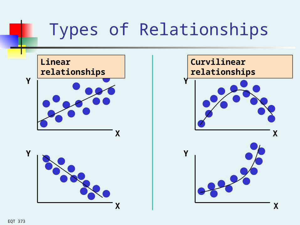
Types of Relationships

Y

X

Y

X

Y

Y

X

X

Linear relationships Curvilinear relationships

EQT 373

Types of Relationships

Y

X

Y

X

Y

Y

X

X

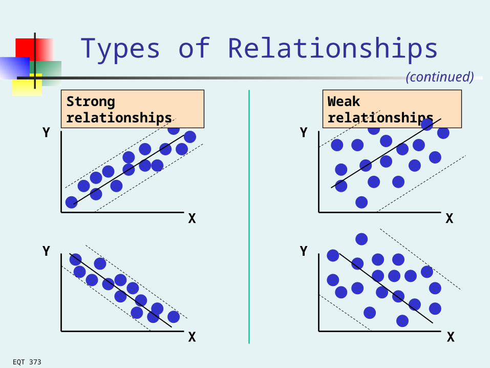
Strong relationships Weak relationships

(continued)

EQT 373

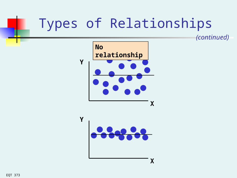
Types of Relationships

Y

X

Y

X

No relationship

(continued)

EQT 373

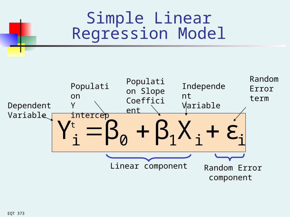
ii10i εXββY Linear component

Simple Linear Regression Model

Population Y intercept

Population SlopeCoefficient

Random Error term

Dependent Variable

Independent Variable

Random Error component

EQT 373

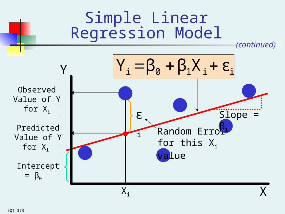
(continued)

Random Error for this Xi value

Y

X

Observed Value of Y for Xi

Predicted Value of Y for Xi

ii10i εXββY

Xi

Slope = β1

Intercept = β0

εi

Simple Linear Regression Model

EQT 373

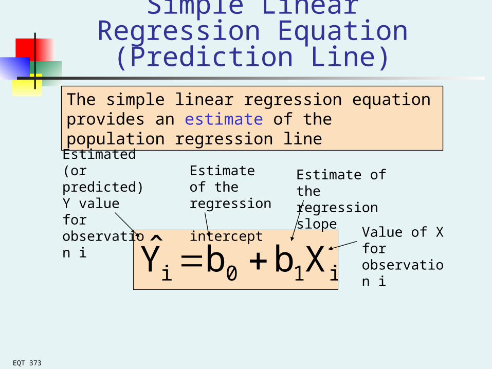
i10i XbbY

The simple linear regression equation provides an estimate of the population regression line

Simple Linear Regression Equation (Prediction Line)

Estimate of the regression

intercept

Estimate of the regression slope

Estimated (or predicted) Y value for observation i

Value of X for observation i

EQT 373

The Least Squares Method

b0 and b1 are obtained by finding the values of

that minimize the sum of the squared differences

between Y and :

2i10i

2ii ))Xb(b(Ymin)Y(Ymin

Y

EQT 373

Finding the Least Squares Equation

The coefficients b0 and b1 , and other regression results in this chapter, will be found using Excel

Formulas are shown in the text for those who are interested

EQT 373

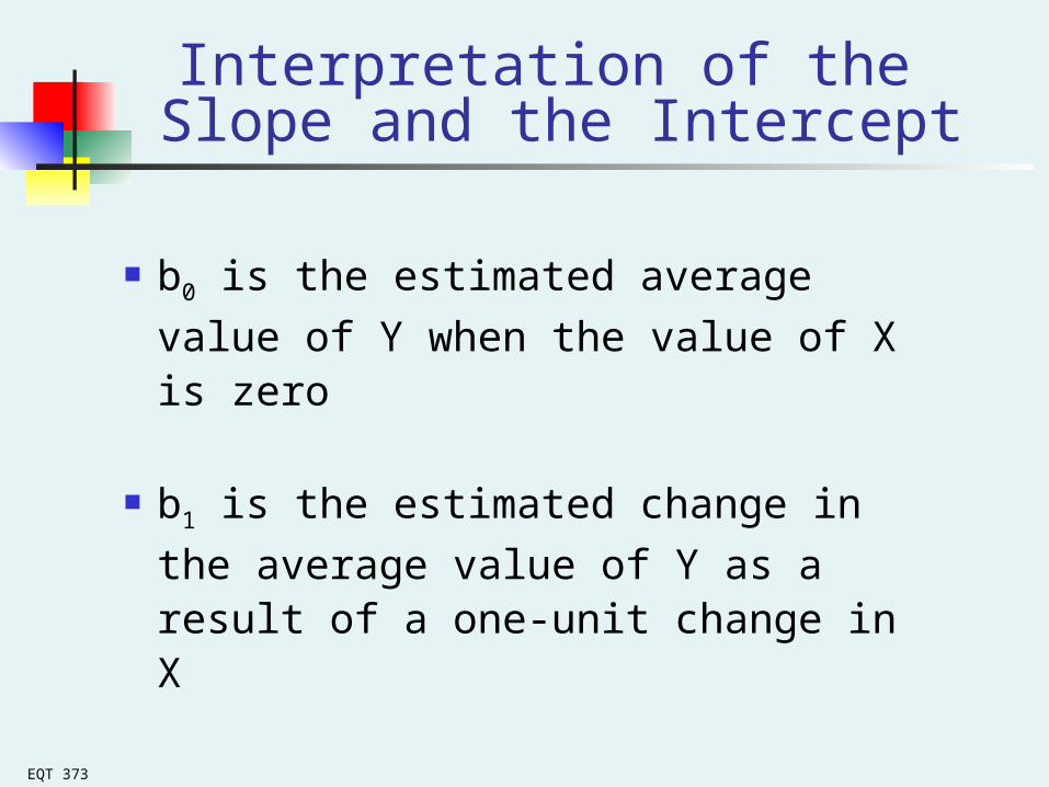
b0 is the estimated average value of Y

when the value of X is zero

b1 is the estimated change in the

average value of Y as a result of a one-unit change in X

Interpretation of the Slope and the Intercept

EQT 373

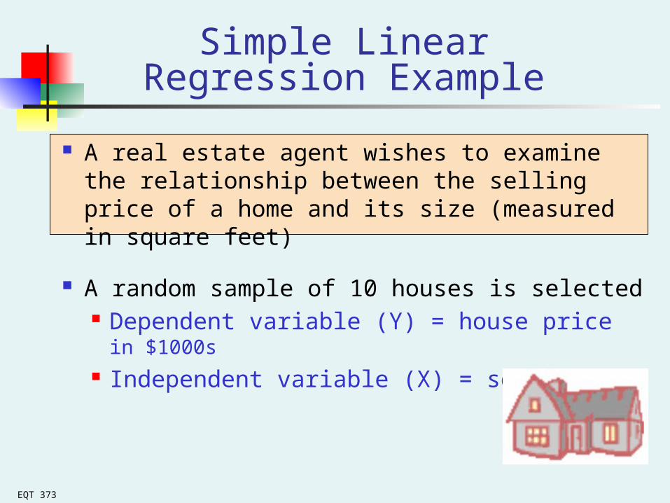
Simple Linear Regression Example

A real estate agent wishes to examine the relationship between the selling price of a home and its size (measured in square feet)

A random sample of 10 houses is selected Dependent variable (Y) = house price in $1000s Independent variable (X) = square feet

EQT 373

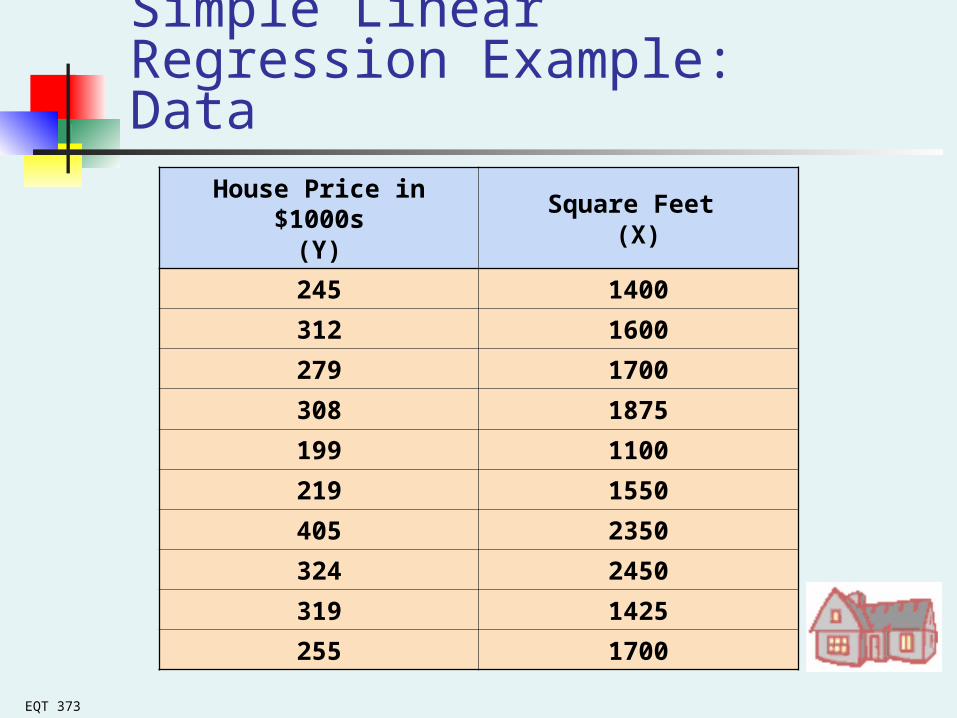
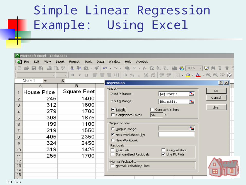
Simple Linear Regression Example: Data

House Price in $1000s(Y)

Square Feet (X)

245 1400

312 1600

279 1700

308 1875

199 1100

219 1550

405 2350

324 2450

319 1425

255 1700

EQT 373

0

50

100

150

200

250

300

350

400

450

0 500 1000 1500 2000 2500 3000

Square Feet

Ho

use

Pri

ce (

$100

0s)

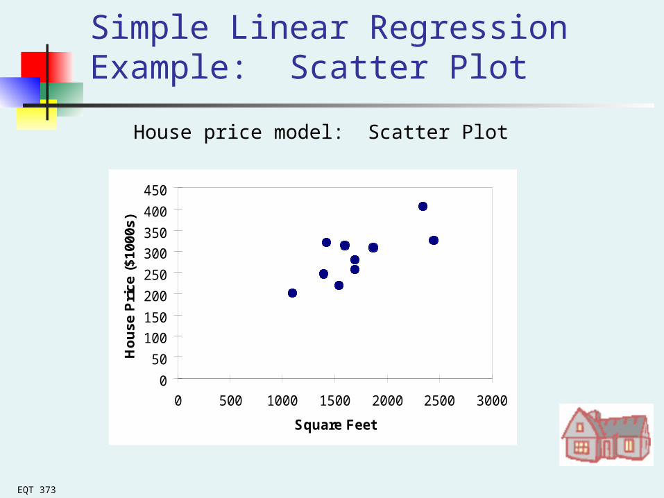
Simple Linear Regression Example: Scatter Plot

House price model: Scatter Plot

EQT 373

Simple Linear Regression Example: Using Excel

EQT 373

Simple Linear Regression Example: Excel Output

Regression Statistics

Multiple R 0.76211

R Square 0.58082

Adjusted R Square 0.52842

Standard Error 41.33032

Observations 10

ANOVA  df SS MS F Significance F

Regression 1 18934.9348 18934.9348 11.0848 0.01039

Residual 8 13665.5652 1708.1957

Total 9 32600.5000      

  Coefficients Standard Error t Stat P-value Lower 95% Upper 95%

Intercept 98.24833 58.03348 1.69296 0.12892 -35.57720 232.07386

Square Feet 0.10977 0.03297 3.32938 0.01039 0.03374 0.18580

The regression equation is:

feet) (square 0.10977 98.24833 price house

EQT 373

0

50

100

150

200

250

300

350

400

450

0 500 1000 1500 2000 2500 3000

Square Feet

Ho

use

Pri

ce (

$100

0s)

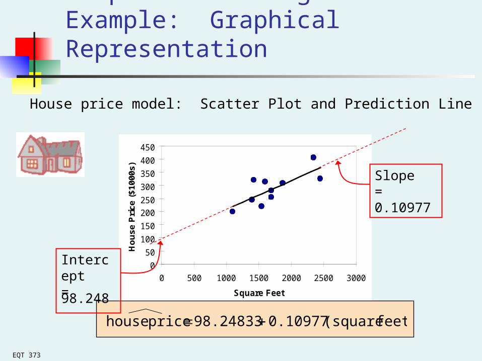
Simple Linear Regression Example: Graphical Representation

House price model: Scatter Plot and Prediction Line

feet) (square 0.10977 98.24833 price house

Slope = 0.10977

Intercept = 98.248

EQT 373

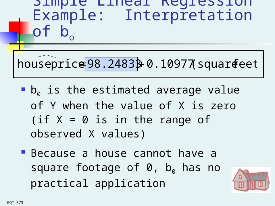
Simple Linear Regression Example: Interpretation of bo

b0 is the estimated average value of Y when the

value of X is zero (if X = 0 is in the range of observed X values)

Because a house cannot have a square footage of 0, b0 has no practical application

feet) (square 0.10977 98.24833 price house

EQT 373

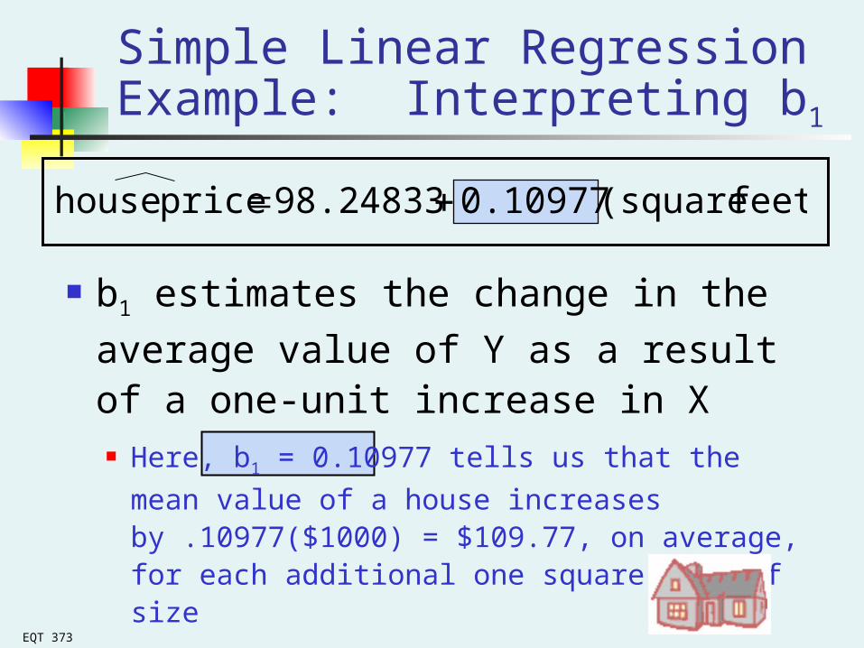
Simple Linear Regression Example: Interpreting b1

b1 estimates the change in the average

value of Y as a result of a one-unit increase in X Here, b1 = 0.10977 tells us that the mean value of a

house increases by .10977($1000) = $109.77, on average, for each additional one square foot of size

feet) (square 0.10977 98.24833 price house

EQT 373

317.85

0)0.1098(200 98.25

(sq.ft.) 0.1098 98.25 price house

Predict the price for a house with 2000 square feet:

The predicted price for a house with 2000 square feet is 317.85($1,000s) = $317,850

Simple Linear Regression Example: Making Predictions

EQT 373

0

50

100

150

200

250

300

350

400

450

0 500 1000 1500 2000 2500 3000

Square Feet

Ho

use

Pri

ce (

$100

0s)

Simple Linear Regression Example: Making Predictions

When using a regression model for prediction, only predict within the relevant range of data

Relevant range for interpolation

Do not try to extrapolate

beyond the range of observed X’s

EQT 373

Measures of Variation

Total variation is made up of two parts:

SSE SSR SST Total Sum of

SquaresRegression Sum

of SquaresError Sum of

Squares

2i )YY(SST 2

ii )YY(SSE 2i )YY(SSR

where:

= Mean value of the dependent variable

Yi = Observed value of the dependent variable

= Predicted value of Y for the given Xi valueiY

Y

EQT 373

SST = total sum of squares (Total Variation)

Measures the variation of the Yi values around their mean Y

SSR = regression sum of squares (Explained Variation)

Variation attributable to the relationship between X and Y

SSE = error sum of squares (Unexplained Variation)

Variation in Y attributable to factors other than X

(continued)

Measures of Variation

EQT 373

(continued)

Xi

Y

X

Yi

SST = (Yi - Y)2

SSE = (Yi - Yi )2

SSR = (Yi - Y)2

_

_

_

Y

Y

Y_Y

Measures of Variation

EQT 373

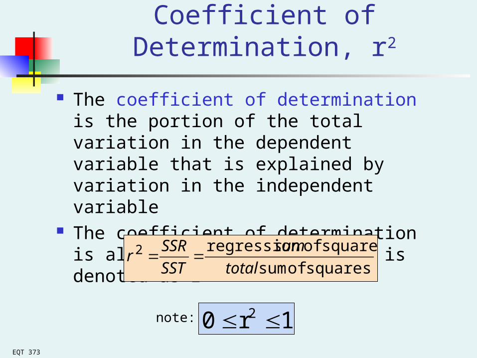
The coefficient of determination is the portion of the total variation in the dependent variable that is explained by variation in the independent variable

The coefficient of determination is also called r-squared and is denoted as r2

Coefficient of Determination, r2

1r0 2 note:

squares of sum

squares of regression2

total

sum

SST

SSRr

EQT 373

r2 = 1

Examples of Approximate r2 Values

Y

X

Y

X

r2 = 1

r2 = 1

Perfect linear relationship between X and Y:

100% of the variation in Y is explained by variation in X

EQT 373

Examples of Approximate r2 Values

Y

X

Y

X

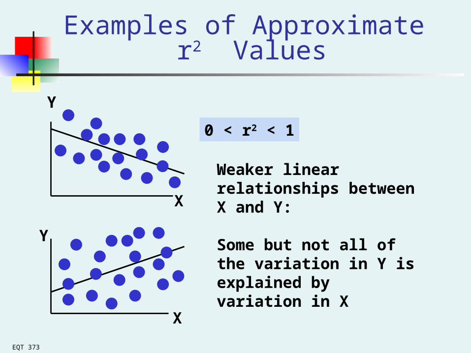
0 < r2 < 1

Weaker linear relationships between X and Y:

Some but not all of the variation in Y is explained by variation in X

EQT 373

Examples of Approximate r2 Values

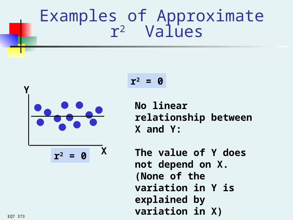
r2 = 0

No linear relationship between X and Y:

The value of Y does not depend on X. (None of the variation in Y is explained by variation in X)

Y

Xr2 = 0

EQT 373

Simple Linear Regression Example: Coefficient of Determination, r2 in Excel

Regression Statistics

Multiple R 0.76211

R Square 0.58082

Adjusted R Square 0.52842

Standard Error 41.33032

Observations 10

ANOVA  df SS MS F Significance F

Regression 1 18934.9348 18934.9348 11.0848 0.01039

Residual 8 13665.5652 1708.1957

Total 9 32600.5000      

  Coefficients Standard Error t Stat P-value Lower 95% Upper 95%

Intercept 98.24833 58.03348 1.69296 0.12892 -35.57720 232.07386

Square Feet 0.10977 0.03297 3.32938 0.01039 0.03374 0.18580

58.08% of the variation in house prices is explained by

variation in square feet

0.5808232600.5000

18934.9348

SST

SSRr 2

EQT 373

Standard Error of Estimate

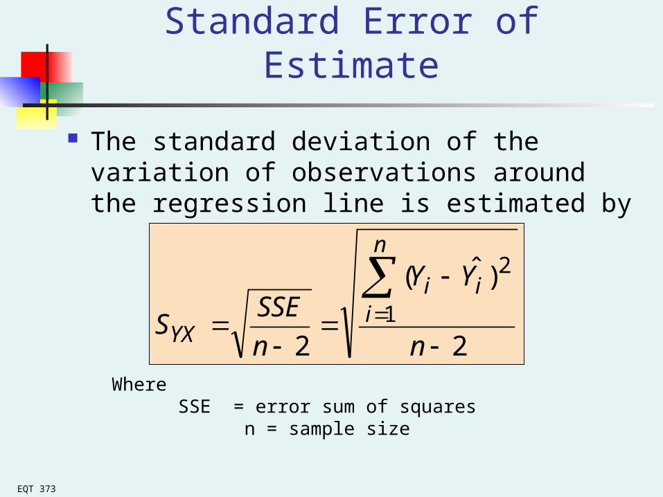
The standard deviation of the variation of observations around the regression line is estimated by

2

)ˆ(

21

2

n

YY

n

SSES

n

iii

YX

WhereSSE = error sum of squares n = sample size

EQT 373

Simple Linear Regression Example:Standard Error of Estimate in Excel

Regression Statistics

Multiple R 0.76211

R Square 0.58082

Adjusted R Square 0.52842

Standard Error 41.33032

Observations 10

ANOVA  df SS MS F Significance F

Regression 1 18934.9348 18934.9348 11.0848 0.01039

Residual 8 13665.5652 1708.1957

Total 9 32600.5000      

  Coefficients Standard Error t Stat P-value Lower 95% Upper 95%

Intercept 98.24833 58.03348 1.69296 0.12892 -35.57720 232.07386

Square Feet 0.10977 0.03297 3.32938 0.01039 0.03374 0.18580

41.33032SYX

EQT 373

Comparing Standard Errors

YY

X XYX

S smallYX

S large

SYX is a measure of the variation of observed Y values from the regression line

The magnitude of SYX should always be judged relative to the size of the Y values in the sample data

i.e., SYX = $41.33K is moderately small relative to house prices in the $200K - $400K range

EQT 373

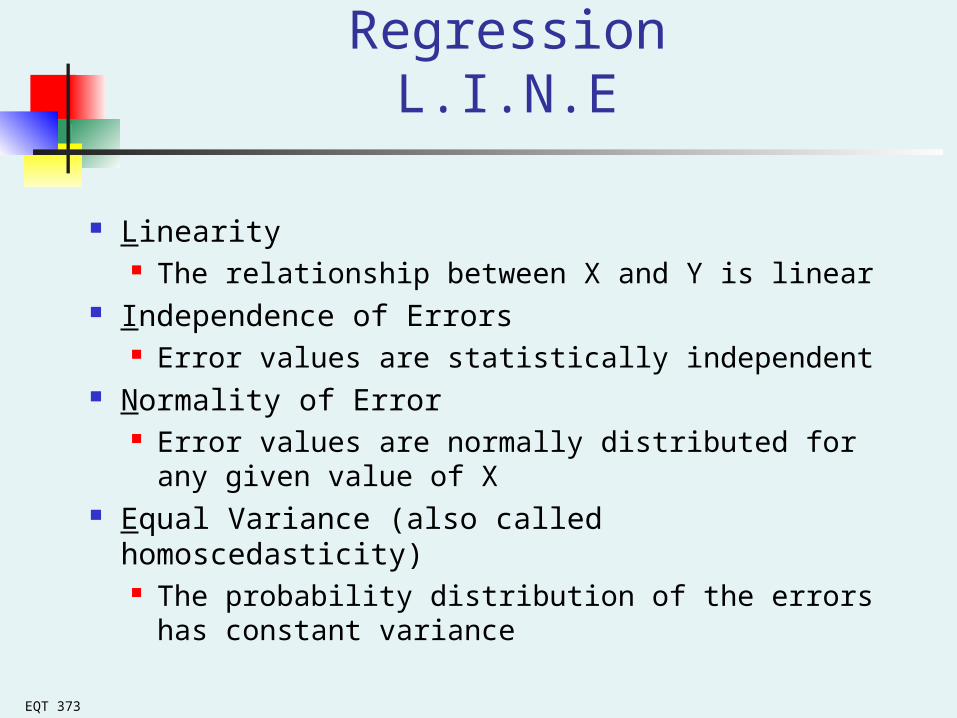
Assumptions of RegressionL.I.N.E

Linearity The relationship between X and Y is linear

Independence of Errors Error values are statistically independent

Normality of Error Error values are normally distributed for any given

value of X Equal Variance (also called homoscedasticity)

The probability distribution of the errors has constant variance

EQT 373

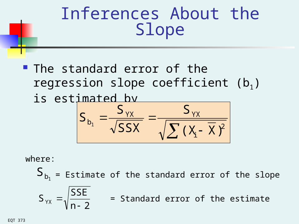
Inferences About the Slope

The standard error of the regression slope coefficient (b1) is estimated by

2i

YXYXb

)X(X

S

SSX

SS

1

where:

= Estimate of the standard error of the slope

= Standard error of the estimate

1bS

2n

SSESYX

EQT 373

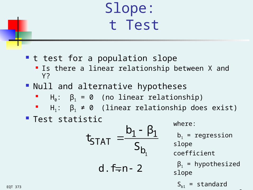
Inferences About the Slope: t Test

t test for a population slope Is there a linear relationship between X and Y?

Null and alternative hypotheses H0: β1 = 0 (no linear relationship) H1: β1 ≠ 0 (linear relationship does exist)

Test statistic

1b

11STAT S

βbt

2nd.f.

where:

b1 = regression slope coefficient

β1 = hypothesized slope

Sb1 = standard error of the slope

EQT 373

Inferences About the Slope: t Test Example

House Price in $1000s

(y)

Square Feet (x)

245 1400

312 1600

279 1700

308 1875

199 1100

219 1550

405 2350

324 2450

319 1425

255 1700

(sq.ft.) 0.1098 98.25 price house

Estimated Regression Equation:

The slope of this model is 0.1098

Is there a relationship between the square footage of the house and its sales price?

EQT 373

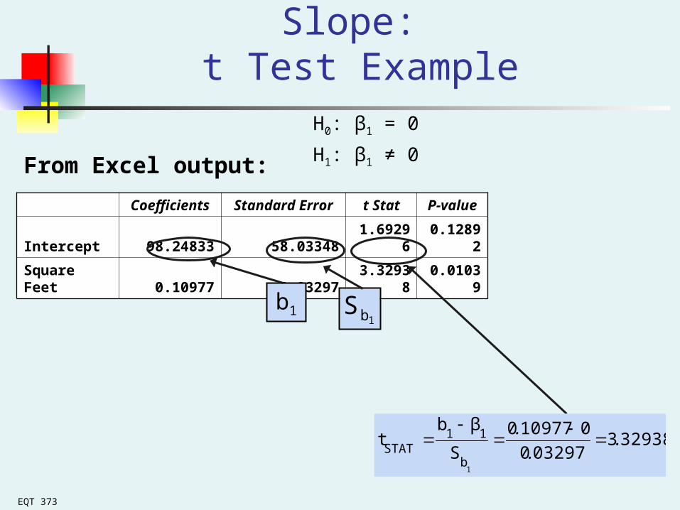
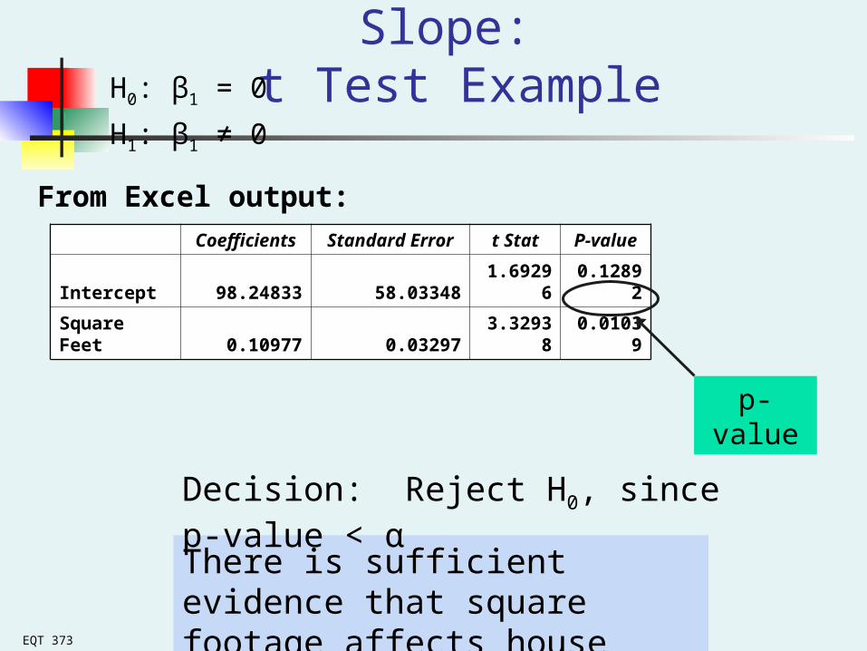
Inferences About the Slope: t Test Example

H0: β1 = 0

H1: β1 ≠ 0From Excel output:

  Coefficients Standard Error t Stat P-value

Intercept 98.24833 58.03348 1.69296 0.12892

Square Feet 0.10977 0.03297 3.32938 0.01039

1bSb1

329383032970

0109770

S

βbt

1b

11STAT

..

.

EQT 373

Inferences About the Slope: t Test Example

Test Statistic: tSTAT = 3.329

There is sufficient evidence that square footage affects house price

Decision: Reject H0

Reject H0Reject H0

/2=.025

-tα/2

Do not reject H0

0 tα/2

/2=.025

-2.3060 2.3060 3.329

d.f. = 10- 2 = 8

H0: β1 = 0

H1: β1 ≠ 0

EQT 373

Inferences About the Slope: t Test ExampleH0: β1 = 0

H1: β1 ≠ 0

From Excel output:   Coefficients Standard Error t Stat P-value

Intercept 98.24833 58.03348 1.69296 0.12892

Square Feet 0.10977 0.03297 3.32938 0.01039

p-value

There is sufficient evidence that square footage affects house price.

Decision: Reject H0, since p-value < α

EQT 373

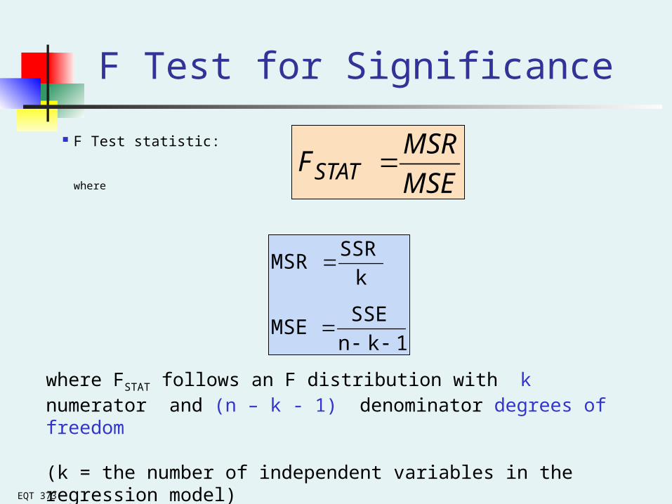
F Test for Significance

F Test statistic:

where

MSE

MSRFSTAT

1kn

SSEMSE

k

SSRMSR

where FSTAT follows an F distribution with k numerator and (n – k - 1) denominator degrees of freedom

(k = the number of independent variables in the regression model)

EQT 373

F-Test for SignificanceExcel Output

Regression Statistics

Multiple R 0.76211

R Square 0.58082

Adjusted R Square 0.52842

Standard Error 41.33032

Observations 10

ANOVA  df SS MS F Significance F

Regression 1 18934.9348 18934.9348 11.0848 0.01039

Residual 8 13665.5652 1708.1957

Total 9 32600.5000      

11.08481708.1957

18934.9348

MSE

MSRFSTAT

With 1 and 8 degrees of freedom

p-value for the F-Test

EQT 373

H0: β1 = 0

H1: β1 ≠ 0

= .05

df1= 1 df2 = 8

Test Statistic:

Decision:

Conclusion:

Reject H0 at = 0.05

There is sufficient evidence that house size affects selling price0

= .05

F.05 = 5.32Reject H0Do not

reject H0

11.08FSTAT MSE

MSR

Critical Value:

F = 5.32

F Test for Significance(continued)

F

EQT 373

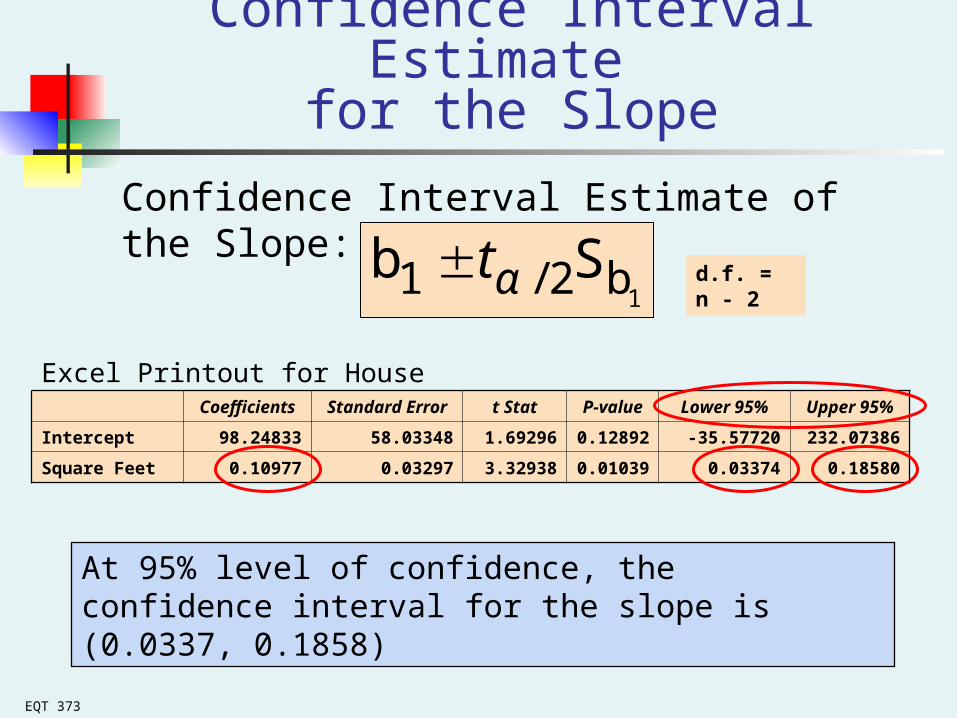
Confidence Interval Estimate for the Slope

Confidence Interval Estimate of the Slope:

Excel Printout for House Prices:

At 95% level of confidence, the confidence interval for the slope is (0.0337, 0.1858)

1b2/1 Sb αt

  Coefficients Standard Error t Stat P-value Lower 95% Upper 95%

Intercept 98.24833 58.03348 1.69296 0.12892 -35.57720 232.07386

Square Feet 0.10977 0.03297 3.32938 0.01039 0.03374 0.18580

d.f. = n - 2

EQT 373

Since the units of the house price variable is $1000s, we are 95% confident that the average impact on sales price is between $33.74 and $185.80 per square foot of house size

  Coefficients Standard Error t Stat P-value Lower 95% Upper 95%

Intercept 98.24833 58.03348 1.69296 0.12892 -35.57720 232.07386

Square Feet 0.10977 0.03297 3.32938 0.01039 0.03374 0.18580

This 95% confidence interval does not include 0.

Conclusion: There is a significant relationship between house price and square feet at the .05 level of significance

Confidence Interval Estimate for the Slope

(continued)

EQT 373

t Test for a Correlation Coefficient

Hypotheses

H0: ρ = 0 (no correlation between X and Y)

H1: ρ ≠ 0 (correlation exists)

Test statistic

(with n – 2 degrees of freedom)

2n

r1

ρ-rt

2STAT

0 b if rr

0 b if rr

where

12

12

EQT 373

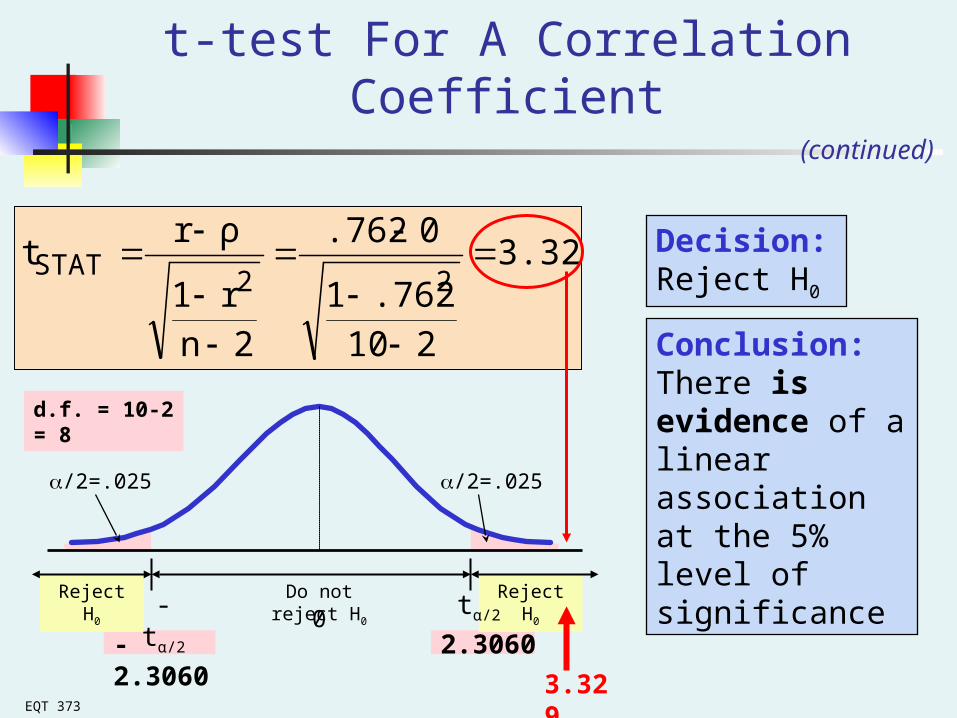
t-test For A Correlation Coefficient

Is there evidence of a linear relationship between square feet and house price at the .05 level of significance?

H0: ρ = 0 (No correlation)

H1: ρ ≠ 0 (correlation exists)

=.05 , df = 10 - 2 = 8

3.329

210

.7621

0.762

2n

r1

ρrt

22STAT

(continued)

EQT 373

t-test For A Correlation Coefficient

Conclusion:There is evidence of a linear association at the 5% level of significance

Decision:Reject H0

Reject H0Reject H0

/2=.025

-tα/2

Do not reject H0

0 tα/2

/2=.025

-2.3060 2.3060

3.329

d.f. = 10-2 = 8

3.329

210

.7621

0.762

2n

r1

ρrt

22STAT

(continued)

EQT 373

Estimating Mean Values and Predicting Individual Values

Y

X Xi

Y = b0+b1Xi

Confidence Interval for the mean of

Y, given Xi

Prediction Interval

for an individual Y, given Xi

Goal: Form intervals around Y to express uncertainty about the value of Y for a given Xi

Y

EQT 373

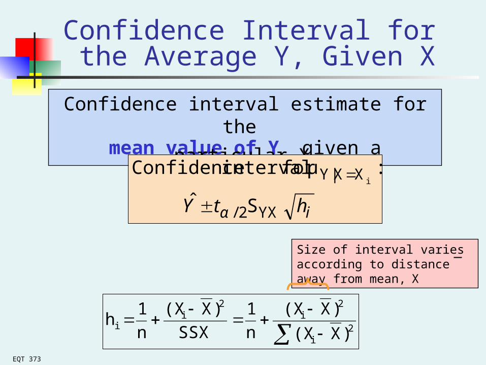
Confidence Interval for the Average Y, Given X

Confidence interval estimate for the mean value of Y given a particular Xi

Size of interval varies according to distance away from mean, X

ihtY YX2/

XX|Y

Sˆ

:μfor interval Confidencei

α

2

i

2i

2i

i)X(X

)X(X

n

1

SSX

)X(X

n

1h

EQT 373

Prediction Interval for an Individual Y, Given X

Confidence interval estimate for an Individual value of Y given a particular Xi

This extra term adds to the interval width to reflect the added uncertainty for an individual case

ihtY

1Sˆ

:Yfor interval Confidence

YX2/

XX i

α

EQT 373

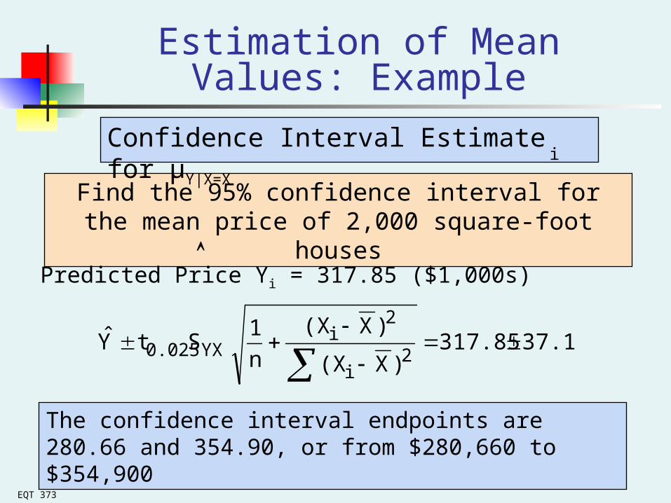
Estimation of Mean Values: Example

Find the 95% confidence interval for the mean price of 2,000 square-foot houses

Predicted Price Yi = 317.85 ($1,000s)

Confidence Interval Estimate for μY|X=X

37.12317.85)X(X

)X(X

n

1StY

2i

2i

YX0.025

The confidence interval endpoints are 280.66 and 354.90, or from $280,660 to $354,900

i

EQT 373

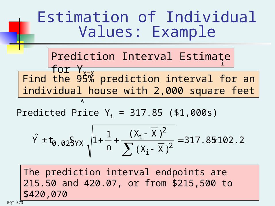
Estimation of Individual Values: Example

Find the 95% prediction interval for an individual house with 2,000 square feet

Predicted Price Yi = 317.85 ($1,000s)

Prediction Interval Estimate for YX=X

102.28317.85)X(X

)X(X

n

11StY

2i

2i

YX0.025

The prediction interval endpoints are 215.50 and 420.07, or from $215,500 to $420,070

i

EQT 373

Finding Confidence and Prediction Intervals in Excel

From Excel, use

PHStat | regression | simple linear regression …

Check the

“confidence and prediction interval for X=”

box and enter the X-value and confidence level desired

EQT 373

Input values

Finding Confidence and Prediction Intervals in Excel

(continued)

Confidence Interval Estimate for μY|X=Xi

Prediction Interval Estimate for YX=Xi

Y

EQT 373

Pitfalls of Regression Analysis

Lacking an awareness of the assumptions underlying least-squares regression

Not knowing how to evaluate the assumptions Not knowing the alternatives to least-squares

regression if a particular assumption is violated Using a regression model without knowledge of

the subject matter Extrapolating outside the relevant range

EQT 373

Strategies for Avoiding the Pitfalls of Regression

Start with a scatter plot of X vs. Y to observe possible relationship

Perform residual analysis to check the assumptions Plot the residuals vs. X to check for violations of

assumptions such as homoscedasticity Use a histogram, stem-and-leaf display, boxplot,

or normal probability plot of the residuals to uncover possible non-normality

EQT 373

Strategies for Avoiding the Pitfalls of Regression

If there is violation of any assumption, use alternative methods or models

If there is no evidence of assumption violation, then test for the significance of the regression coefficients and construct confidence intervals and prediction intervals

Avoid making predictions or forecasts outside the relevant range

(continued)

EQT 373

Chapter Summary

Introduced types of regression models Reviewed assumptions of regression and

correlation Discussed determining the simple linear

regression equation Described measures of variation Discussed residual analysis Addressed measuring autocorrelation

EQT 373

Chapter Summary

Described inference about the slope Discussed correlation -- measuring the strength

of the association Addressed estimation of mean values and

prediction of individual values Discussed possible pitfalls in regression and

recommended strategies to avoid them

(continued)