eoa, inc. memorandum - scvurppp-w2k.com (screen tool case study… · c:\jeff\eoa\current\case...
TRANSCRIPT

C:\JEFF\EOA\current\case study.doc 1 EOA, Inc.
EOA, Inc. MEMORANDUM TO: Santa Clara Valley Urban Runoff Pollution Prevention Program FROM: Jeff Soller and Adam Olivieri SUBJECT: Microbial Risk Screening Tool: Case Study TASK: SC20-02: Microbial Indicators and Effects on Beneficial Uses DATE: March 30, 2001 Abstract The primary objective of this project was to create a computer-based program that can be used to assess the relative microbial risks to public health from recreational exposure to urban creek waters. Given the complexities associated with interpreting bacterial indicator data, a program was developed that can be used on a screening level to streamline the process of evaluating the relative microbial risks to public health from exposure to urban creek waters. The background for and development of the microbial risk screening tool (screening tool) is described in detail under separate cover (Soller and Olivieri, 2001). This memorandum illustrates the utility of the screening tool through a case study example. The case study described herein is based on bacterial indicator data (fecal coliform, total coliform, enterococcus, and fecal streptococcus) collected between 1995 and 1998 from a creek in Santa Clara County in northern California. The results of the case study indicate that each of the indicators yield slightly different estimates of risk to public health. For total and fecal coliform the median risk is estimated to be one and three illness per 1000 recreators, respectively. For enterococcus and fecal streptococcus, the median risk estimate was slightly higher; 10 and 11 per 1000, respectively. Given the variability inherent in environmental data and the uncertainty associated with the relationships between bacterial indicators and pathogens, the variability in the results is not unexpected. It is anticipated that the microbial risk screening tool will be used by public agencies to facilitate the interpretation of microbial indicator or pathogen data with respect to impairment of beneficial uses. With that in mind, it should be clear that risk management decisions will need to consider use levels (how many recreators, where, when) in addition to characterizing the risk levels that are associated with recreating in a given water body as estimated by bacterial indicator data. Introduction In response to sample data showing possible exceedances of water-quality criteria for fecal coliform in various Bay Area creeks, a computer-based tool was created

C:\JEFF\EOA\current\case study.doc 2 EOA, Inc.
that can be used to evaluate the relative microbial risks to public health. The background for and development of the microbial risk screening tool is described in detail under separate cover (Soller and Olivieri, 2001). This Memorandum illustrates the utility of the microbial risk screening tool through a case study example. The case study described herein is based on bacterial indicator data collected between 1995 and 1998 from a creek in Santa Clara County. The four indicator organisms monitored in the creek were total and fecal coliform, fecal streptococcus, and enterococcus. Water quality criteria objectives are specified in the CA RWQCB San Francisco Bay Region Water Quality Control Plan (RWQCB, 1995) for total and fecal coliform bacteria for water contact recreation, shellfish harvesting, non-contact water recreation, and municipal supply beneficial uses. Additionally, US EPA specify bacteriological criteria for freshwater water contact recreation for enterococcus and E. coli (US EPA, 1986). For water contact recreation, the Basin Plan objectives and fresh water criteria are summarized in Table 1. A summary of how these criteria were established are summarized under separate cover (US EPA, 1986; EOA, Inc., 1999).
Table 1: Water Quality Criteria for Indicator Organisms Organism Criteria Value UnitsFecal Coliform log mean <200 MPN/100 ml
90th %ile <400Total Coliform median <240 MPN/100 ml
maximum <10,000Enterococci steady state 33 colonies/100ml
max at beach 61max at lightly used area 108
E Coli steady state 126 colonies/100mlmax at beach 235max at lightly used area 406
This Memorandum illustrates how the microbial risk screening tool may be used to estimate a distribution of human health risk from recreational exposure to urban creek waters. Presented below are case study results for fecal coliform, total coliform, enterococcus, and fecal streptococcus data for the Santa Clara County creek. Also presented is a comparison between those results and the Basin Plan objectives and fresh water criteria specified above. Program Input Environmental data Urban creek data were monitored for bacterial indicators between November 1995 and August 1998. The data collection attempted to characterize the variation in bacteriological levels in the creek as a function of location, time of year, and time of day. Ten in-stream surface water locations and five storm sewer outfalls that discharge to the creek were monitored. This monitoring included both

C:\JEFF\EOA\current\case study.doc 3 EOA, Inc.
undeveloped and developed residential areas. Four bacterial indicator organisms were monitored: total and fecal coliform, fecal streptococcus, and enterococcus. Data screening Preliminary data testing was performed prior to running the microbial risk screening tool by grouping the data first by location and then by date. Data were grouped by location into two groups, the in-stream sampling points and the storm sewer outfalls. A Mann-Whitney Test was performed to determine if these sets of data were significantly different. The results are shown in Tables 2 and 3. Table 2 shows the ranking for the two location groups for each of the indicators studied. Location 1 is the data from the in-stream locations; location 2 is the data from the storm sewer outfall locations. N is the number of data points collected. Ranking was done separately for each indicator organism, as shown in Table 2. Table 3 shows the results of the Mann-Whitney test for the two sets of locations. Each of the indicators reveals the same result: because the significance is small (in this case it is 0.000), it may be inferred that in-stream data points are significantly different from the storm sewer data points. Therefore, only the data that are consistent with the actual exposure scenarios, the in-stream data, are used in subsequent analyses.
Table 2: Ranking the Location Data for use in the Mann-Whitney Test
Table 3: Mann-Whitney Test Statistics for Location Data
342 190.50 65152.5093 319.11 29677.50
435342 192.44 65814.5093 311.99 29015.50
435342 191.83 65606.0091 311.59 28355.00
433342 188.60 64501.5093 326.11 30328.50
435
LOCCODE12Total12Total12Total12Total
FecalColiform
Fecal Strep
Enterococci
TotalColiform
NMeanRank
Sum ofRanks
Ranks
6499.500 7161.500 6953.000 5848.50065152.500 65814.500 65606.000 64501.500
-8.761 -8.134 -8.115 -9.369.000 .000 .000 .000
Mann-Whitney UWilcoxon WZAsymp. Sig. (2-tailed)
FECCOLIF FECSTREP ENTEROC TOTCOLIF
C:\JEFF\EOA\current\case study.doc 4 EOA, Inc.
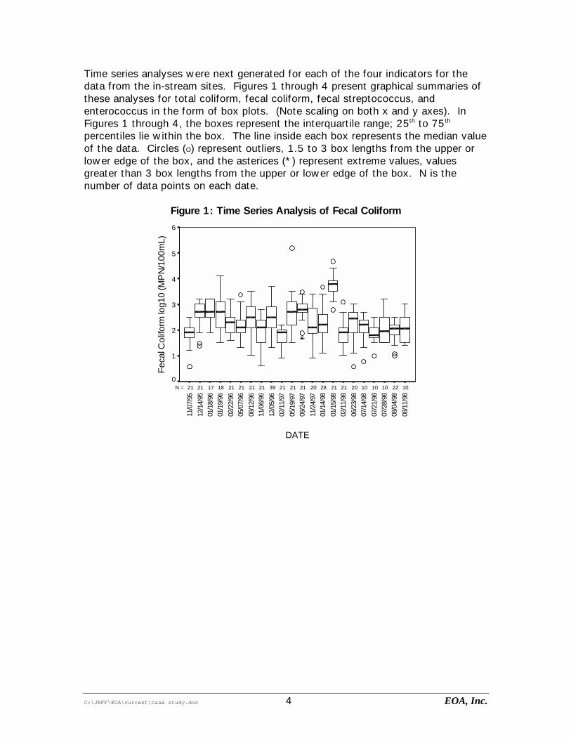
Time series analyses were next generated for each of the four indicators for the data from the in-stream sites. Figures 1 through 4 present graphical summaries of these analyses for total coliform, fecal coliform, fecal streptococcus, and enterococcus in the form of box plots. (Note scaling on both x and y axes). In Figures 1 through 4, the boxes represent the interquartile range; 25th to 75th percentiles lie within the box. The line inside each box represents the median value of the data. Circles (O) represent outliers, 1.5 to 3 box lengths from the upper or lower edge of the box, and the asterices (*) represent extreme values, values greater than 3 box lengths from the upper or lower edge of the box. N is the number of data points on each date.
Figure 1: Time Series Analysis of Fecal Coliform
10221010102021212820212121392121212118172121N =
DATE
08/1
1/98
08/0
4/98
07/2
8/98
07/2
1/98
07/1
4/98
06/2
3/98
02/1
1/98
01/1
5/98
01/1
4/98
11/2
4/97
09/2
4/97
05/1
9/97
02/1
1/97
12/0
5/96
11/0
6/96
08/1
2/96
05/0
7/96
02/2
2/96
01/1
9/96
01/1
8/96
12/1
4/95
11/0
7/95
Feca
l Col
iform
log1
0 (M
PN/1
00m
L)
6
5
4
3
2
1
0

C:\JEFF\EOA\current\case study.doc 5 EOA, Inc.
Figure 2: Time Series Analysis of Total Coliform
10221010102021212820212121392121212118172121N =
DATE
08/1
1/98
08/0
4/98
07/2
8/98
07/2
1/98
07/1
4/98
06/2
3/98
02/1
1/98
01/1
5/98
01/1
4/98
11/2
4/97
09/2
4/97
05/1
9/97
02/1
1/97
12/0
5/96
11/0
6/96
08/1
2/96
05/0
7/96
02/2
2/96
01/1
9/96
01/1
8/96
12/1
4/95
11/0
7/95
Tota
l Col
iform
log1
0 (M
PN/1
00m
L)
6
5
4
3
2
1
0
Figure 3: Time Series Analysis of Enterococcus
10221010102021212820212121392121212116172121N =
DATE
08/1
1/98
08/0
4/98
07/2
8/98
07/2
1/98
07/1
4/98
06/2
3/98
02/1
1/98
01/1
5/98
01/1
4/98
11/2
4/97
09/2
4/97
05/1
9/97
02/1
1/97
12/0
5/96
11/0
6/96
08/1
2/96
05/0
7/96
02/2
2/96
01/1
9/96
01/1
8/96
12/1
4/95
11/0
7/95
Ente
roco
ccus
log1
0 (c
fu/1
00m
l)
6
5
4
3
2
1
0
-1

C:\JEFF\EOA\current\case study.doc 6 EOA, Inc.
Figure 4: Time Series Analysis of Fecal Streptococcus
10221010102021212820212121392121212118172121N =
DATE
08/1
1/98
08/0
4/98
07/2
8/98
07/2
1/98
07/1
4/98
06/2
3/98
02/1
1/98
01/1
5/98
01/1
4/98
11/2
4/97
09/2
4/97
05/1
9/97
02/1
1/97
12/0
5/96
11/0
6/96
08/1
2/96
05/0
7/96
02/2
2/96
01/1
9/96
01/1
8/96
12/1
4/95
11/0
7/95
Feca
l Stre
p lo
g10
(cfu
/100
mL)
5
4
3
2
1
0
-1
Inspection of Figures 1 through 4 reveals that for all four indicators, the data are scattered and no significant trends seem to exist throughout the year. In the ensuing analysis data for all of the in-stream sites are grouped for each individual indicator. Hence, this study comprises four data sets, one for each indicator (and excludes data collected from the storm sewer outfalls). Health effects The microbial risk screening tool estimates the distribution of risk to human health for recreational exposure to pathogens in a freshwater environment. Given a set of bacteriological indicator or pathogen data, the screening tool outputs an estimated distribution of risk to human health. The background, development, and basis for the screening tool are described in detail under separate cover (EOA, Inc., 2000). The screening tool takes as input, bacteriological indicator or pathogen data including the following: total coliform, fecal coliform, fecal streptococcus, F+RNA coliphage, E. coli, enterococcus, giardia spp., and cryptosporidium parvum. For F+RNA coliphage, fecal coliform, total coliform, and fecal streptococcus, the program first converts indicator concentration data to an “equivalent” pathogen concentration (based on translation functions derived via literature review). Using the appropriate dose-response equation and a distribution for ingestion, the pathogen concentration distributions are then converted to a distribution of risk based on a series of Monte Carlo simulations. For E. coli and enterococcus, the indicator concentration distributions are converted directly to risk via simulation using the dose-response equations developed by the US EPA (1986) and a distribution of ingestion. Giardia spp. and cryptosporidium parvum are pathogenic to humans and, therefore, are converted directly to health

C:\JEFF\EOA\current\case study.doc 7 EOA, Inc.
risk via simulations using the appropriate dose-response equations, and the distribution of ingestion. The following assumptions are embedded into the microbial risk screening tool (EOA, Inc., 2000):
• Bacterial indicator or pathogen data are obtained from an urban freshwater environment;
• The data input are representative of the water body under study, and any preliminary data screening has been carried out prior to inputting the data into the screening tool. The existence of outliers may impact the results of the computations carried out in the screening tool, and data not considered representative must be removed prior to running the program;
• Exposure to pathogens occurs through recreational contact (i.e. swimming). If other routes of exposure are significant, the screening tool may not be suitable;
• Exposure events are independent, and results of the screening tool estimate the relative risk associated with a single exposure event;
• The primary risk from recreational exposure to pathogens is to enteric viruses;
• Factors not accounted for include person to person transmission of disease, immunity (protection from infection due to prior exposure), and differential susceptibility within the population;
• Ingestion is estimated as a lognormal distribution with mean of 50 mL and 90% of the data between 25 and 75mL;
• The output from the program is the estimated distribution of risk to enteric virus infection per person per exposure event (when giardia spp. or cryptosporidium parvum data are input the output risk is to those pathogens), and
• This program is intended only as a screening tool to determine if further investigations of health risk are appropriate.
Those readers interested in more detail are referred to the program documentation (Soller and Olivieri, 2001). Results of Case Study Risk distributions associated with exposure to microbial pathogens were estimated using the screening tool. The four bacteriological indicators monitored were total and fecal coliform, enterococcus, and fecal streptococcus. A summary of the indicator concentration data is presented in Table 4. Inspection of Table 4 reveals that the data were right skewed for each of the indicators (mean > median). Therefore for each of the indicators, concentration data were fit to lognormal distributions using the method of maximum likelihood.

C:\JEFF\EOA\current\case study.doc 8 EOA, Inc.
Table 4: Summary of Indicator Concentration Data
Concentration Indicator
Number of samples
Mean
Median
Fecal coliform 342 833 130 Total coliform 342 1280 300 Enterococcus 342 219 85 Fecal streptococcus 342 283 120
Enterococcus Figures 5a and 5b show the output from the microbial risk screening tool for enterococcus data. Output from the program also includes the assumptions that are used in the program to generate the results. For the enterococcus results shown in Figures 5a and 5b, those assumptions are found in Appendix A. Shown in the first graph in Figure 5a are the observed concentration data shown as a histogram and the corresponding maximum likelihood estimate shown as a line graph. Note that the concentration axis is shown on a log scale. The second graph shown in Figure 5a (Graph B upper right) shows the ingestion rate distribution per person per event. This distribution is derived from the generally accepted volume of water ingested during recreational activities (50 mL). The ingestion is modeled as a lognormal distribution with a mean of 50 mL and with 90 percent of the ingestion events occurring between 25 and 75 mL. Graph C (middle left) in Figure 5a shows the distribution of dose. For enterococcus, "Distribution of Dose" refers to the expected distribution of indicator organisms ingested per recreational event. Graph D (middle right) in Figure 5a displays the dose-response function for enterococcus (US EPA, 1986): Y = -6.278 + 9.40 log (x) where Y is the illness rate per 1000 swimmers and x is the enterococcus density per 100 mL. Graphs E and F (bottom) in Figure 5a show the resultant distribution of risk and the cumulative distribution of risk, respectively, per person per exposure event. The results shown in Graphs E and F are the result of a series of simulations which sampled the distributions described above. To display of the majority of the data in the clearest way, the upper 5% of the distribution is truncated and not shown in graph E. Graph F shows the full cumulative distribution of risk. For enterococcus in this case study, the estimated risk distribution has a median of 10 illnesses per 1000 people exposed, and a 95th percentile of 22 illnesses per 1000 people exposed.
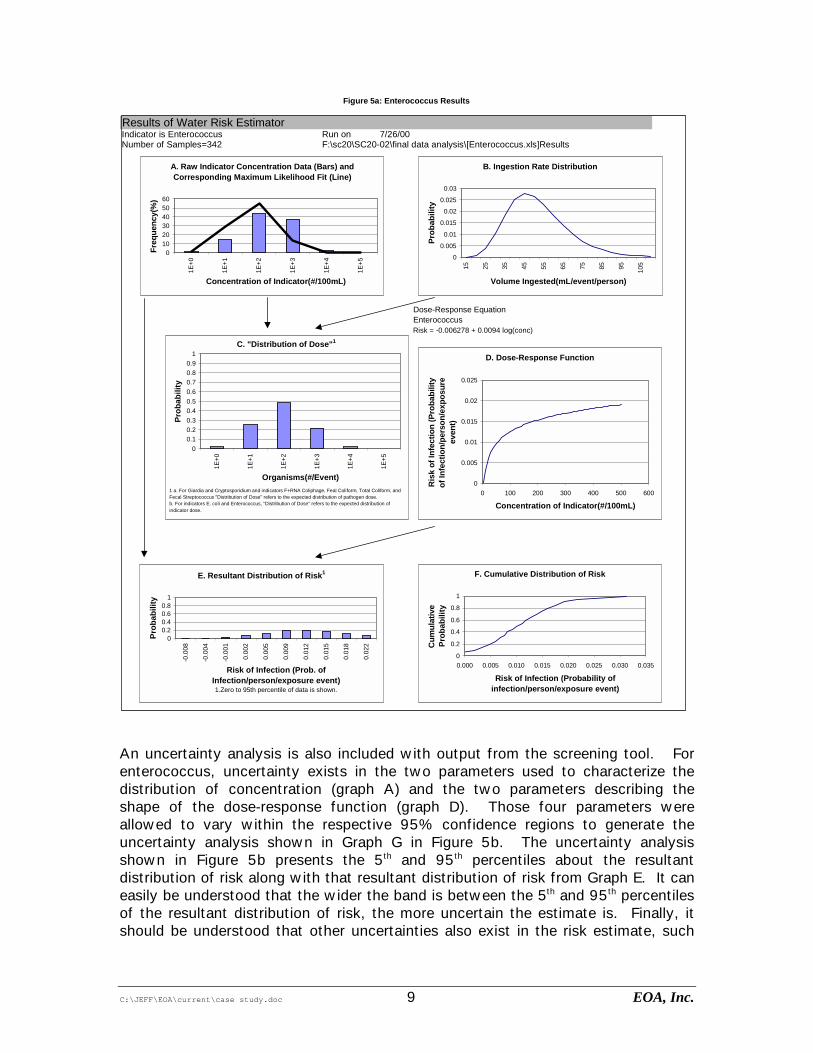
C:\JEFF\EOA\current\case study.doc 9 EOA, Inc.
Results of Water Risk EstimatorIndicator is Enterococcus Run on 7/26/00Number of Samples=342 F:\sc20\SC20-02\final data analysis\[Enterococcus.xls]Results
Dose-Response EquationEnterococcusRisk = -0.006278 + 0.0094 log(conc)
Figure 5a: Enterococcus Results
A. Raw Indicator Concentration Data (Bars) and Corresponding Maximum Likelihood Fit (Line)
0102030405060
1E+0
1E+1
1E+2
1E+3
1E+4
1E+5
Concentration of Indicator(#/100mL)
Freq
uenc
y(%
)B. Ingestion Rate Distribution
0
0.005
0.01
0.015
0.02
0.025
0.03
15 25 35 45 55 65 75 85 95 105
Volume Ingested(mL/event/person)
Prob
abili
ty
C. "Distribution of Dose"1
00.10.20.30.40.50.60.70.80.9
1
1E+0
1E+1
1E+2
1E+3
1E+4
1E+5
Organisms(#/Event)
Prob
abili
ty
1 a. For Giardia and Cryptosporidium and indicators F+RNA Coliphage, Feal Coliform, Total Coliform, and Fecal Streptococcus "Distribution of Dose" refers to the expected distribution of pathogen dose.b. For indicators E. coli and Enterococcus, "Distribution of Dose" refers to the expected distribution of indicator dose.
E. Resultant Distribution of Risk1
00.20.40.60.8
1
-0.0
08
-0.0
04
-0.0
01
0.00
2
0.00
5
0.00
9
0.01
2
0.01
5
0.01
8
0.02
2
Risk of Infection (Prob. of Infection/person/exposure event)1.Zero to 95th percentile of data is shown.
Prob
abili
ty
F. Cumulative Distribution of Risk
0
0.2
0.4
0.6
0.8
1
0.000 0.005 0.010 0.015 0.020 0.025 0.030 0.035
Risk of Infection (Probability of infection/person/exposure event)
Cum
ulat
ive
Prob
abili
ty
D. Dose-Response Function
0
0.005
0.01
0.015
0.02
0.025
0 100 200 300 400 500 600
Concentration of Indicator(#/100mL)
Ris
k of
Infe
ctio
n (P
roba
bilit
y of
Infe
ctio
n/pe
rson
/exp
osur
e ev
ent)
An uncertainty analysis is also included with output from the screening tool. For enterococcus, uncertainty exists in the two parameters used to characterize the distribution of concentration (graph A) and the two parameters describing the shape of the dose-response function (graph D). Those four parameters were allowed to vary within the respective 95% confidence regions to generate the uncertainty analysis shown in Graph G in Figure 5b. The uncertainty analysis shown in Figure 5b presents the 5th and 95th percentiles about the resultant distribution of risk along with that resultant distribution of risk from Graph E. It can easily be understood that the wider the band is between the 5th and 95th percentiles of the resultant distribution of risk, the more uncertain the estimate is. Finally, it should be understood that other uncertainties also exist in the risk estimate, such

C:\JEFF\EOA\current\case study.doc 10 EOA, Inc.
as the uncertainty in the analytical results. However other uncertainties are more difficult to quantify than those accounted for in the screening tool.
Figure 5b: Enterococcus Uncertainty Analysis
G. Uncertainty of Risk
00.10.20.30.40.50.60.70.80.9
1
-0.01
-0.01 0.0
00.0
00.0
10.0
20.0
20.0
30.0
40.0
4
Risk of Infection (Probability of Infection/person/exposure event)
Prob
abili
ty95th %ile of Risk
Maximum Likelihood RiskDistribution5th %ile of Risk
Fecal Coliform The risk to public health associated with the fecal coliform monitoring results is estimated in a manner analogous to that presented above for enterococcus. Output from the screening tool is presented in Figures 6a and 6b. The assumptions associated with those results for fecal coliform are found in Appendix B. Shown in Figure 6a Graph A are the observed concentration data (histogram) and the corresponding maximum likelihood estimate (line graph). The second graph shown in Figure 6a (Graph B upper right) shows the ingestion rate distribution per person per event. Graph C (middle left) in Figure 6a presents the distribution of dose, which for fecal coliform, refers to the expected distribution of pathogens (viruses) ingested1 per recreational event. Graph D (middle right) in Figure 6a displays the appropriate dose-response function2 (Ward, et al., 1986 and Haas, 1983):
r = 1 – (1 + y/b)^(-a)
where r is the risk of infection per person per exposure event, y is the dose of viruses ingested, and a and b are 0.26 and 0.42, the parameters of the dose-response function. This dose-response function is also used for total coliform and fecal streptococcus. Graphs E and F (bottom) in Figure 6a show the resultant distribution of risk and the cumulative distribution of risk, respectively, per person per exposure event. For fecal coliform in this case study, the estimated risk distribution has a median of 3
1 Those readers interested in the procedures used to translate indicator data to pathogen data are referred to EOA, 2000. 2 It is assumed that risk from recreational activities is mainly derived from ingestion of human infectious viruses, and that those viruses are conservatively characterized by using the dose-response for rotavirus.

C:\JEFF\EOA\current\case study.doc 11 EOA, Inc.
illnesses per 1000 people exposed, and a 95th percentile of 128 illnesses per 1000 people exposed. The uncertainty analysis for fecal coliform is slightly different than that performed for enterococcus. For fecal coliform, uncertainty exists in the two parameters used to calculate the distribution of concentration (Graph A), the two parameters describing the shape of the dose-response function (Graph D), and the two parameters describing the relationship between indicator and pathogen concentration (not shown). These six parameters are varied in the uncertainty analysis, the results of which are shown in Graph G in Figure 6b. In Figure 6b, the 5th and 95th percentiles about the resultant risk along with the distribution of risk from Graph E are presented.
Results of Water Risk EstimatorIndicator is Fecal Coliform Run on 7/26/00Number of Samples=342 F:\sc20\SC20-02\final data analysis\[Fecal Coliform.xls]Results
Dose-Response EquationFecal ColiformRisk = 1 - (1+(dose/0.42))^(-0.26)
Figure6a: Fecal Coliform Results
A. Raw Indicator Concentration Data (Bars) and Corresponding Maximum Likelihood Fit (Line)
010203040506070
1E+0
1E+1
1E+2
1E+3
1E+4
1E+5
Concentration of Indicator(#/100mL)
Freq
uenc
y(%
)
B. Ingestion Rate Distribution
0
0.005
0.01
0.015
0.02
0.025
0.03
15 25 35 45 55 65 75 85 95 105
Volume Ingested(mL/event/person)
Prob
abili
ty
C. "Distribution of Dose"1
00.10.20.30.40.50.60.70.80.9
1
0.02
9
0.05
9
0.08
8
0.11
7
0.14
6
0.17
6
0.20
5
0.23
4
0.26
3
0.29
3
Organisms(#/Event)
Prob
abili
ty
1 a. For Giardia and Cryptosporidium and indicators F+RNA Coliphage, Feal Coliform, Total Coliform, and Fecal Streptococcus, "Distribution of Dose" refers to the expected distribution of pathogen dose.b. For indicators E. coli and Enterococcus, "Distribution of Dose" refers to the expected distribution of indicator dose.c.Zero to 95th percentile of data is shown.
E. Resultant Distribution of Risk1
00.20.40.60.8
1
0.01
0.03
0.04
0.05
0.06
0.08
0.09
0.10
0.12
0.13
Risk of Infection (Prob. of Infection/person/exposure event)1.Zero to 95th percentile of data is shown.
Prob
abili
ty
F. Cumulative Distribution of Risk
0
0.2
0.4
0.6
0.8
1
0.000 0.100 0.200 0.300 0.400 0.500
Risk of Infection (Probability of infection/person/exposure event)
Cum
ulat
ive
Prob
abili
ty
D. Dose-Response Function
0
0.1
0.2
0.3
0.4
0.5
0.6
0.7
0.8
0.9
0 100 200 300 400 500 600
Organisms(#/event)
Ris
k of
Infe
ctio
n (P
roba
bilit
y of
Infe
ctio
n/pe
rson
/exp
osur
e ev
ent)

C:\JEFF\EOA\current\case study.doc 12 EOA, Inc.
Figure 6b: Fecal Coliform Uncertainty Analysis
G. Uncertainty of Risk
00.10.20.30.40.50.60.70.80.9
1
0.05
0.14
0.23
0.32
0.41
0.51
0.60
0.69
0.78
0.88
Risk of Infection (Probability of Infection/person/exposure event)
Prob
abili
ty
95th %ile of Risk
Maximum Likelihood RiskDistribution5th %ile of Risk
Total Coliform The risk to public health associated with the total coliform monitoring results is estimated in a manner most analogous to that presented above for fecal coliform. Output from the screening tool for total coliform is presented in Figures 7a and 7b. The assumptions associated with those results for total coliform are found in Appendix C. The observed total coliform concentration data and the corresponding maximum likelihood estimate are presented in Figure 7a Graph A. The second graph shown in Figure 7a (Graph B upper right) shows the ingestion rate distribution per person per event. Graph C (middle left) in Figure 7a presents the distribution of dose, which for total coliform, refers to the expected distribution of pathogens (viruses) ingested per recreational event. To estimate the expected distribution of viruses, total coliform are first converted to a fecal coliform equivalent. A site specific translation may be used if data are available, otherwise the default value of 0.18 is used, based on US EPA data (US EPA, 1986). The “fecal coliform equivalent” is then converted to an equivalent concentration of viruses as described in the previous section. Graph D (middle right) in Figure 6a displays the appropriate dose-response function, as previously described. Graphs E and F (bottom) in Figure 7a show the resultant distribution of risk and the cumulative distribution of risk, respectively, per person per exposure event. As described previously, only the lower 95 percent of the data are shown in Graph E. For total coliform in this case study, the estimated risk distribution has a median of 1 illness per 1000 people exposed, and a 95th percentile of 29 illnesses per 1000 people exposed. The uncertainty analysis for total coliform is similar to that performed for fecal coliform. For total coliform, uncertainty exists in the two parameters used to calculate the distribution of concentration (Graph A), the two parameters describing the shape of the dose-response function (Graph D), and the two parameters describing the relationship between indicator and pathogen concentration (not shown). These six parameters are varied in the uncertainty analysis, the results of which are shown in Graph G in Figure 7b.
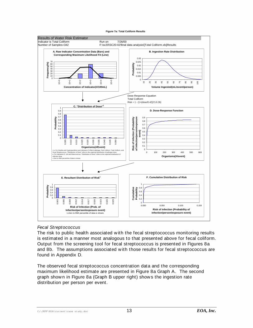
C:\JEFF\EOA\current\case study.doc 13 EOA, Inc.
Results of Water Risk EstimatorIndicator is Total Coliform Run on 7/26/00Number of Samples=342 F:\sc20\SC20-02\final data analysis\[Total Coliform.xls]Results
Dose-Response EquationTotal ColiformRisk = 1 - (1+(dose/0.42))^(-0.26)
Figure 7a: Total Coliform Results
A. Raw Indicator Concentration Data (Bars) and Corresponding Maximum Likelihood Fit (Line)
010203040506070
1E+0
1E+1
1E+2
1E+3
1E+4
1E+5
Concentration of Indicator(#/100mL)
Freq
uenc
y(%
)B. Ingestion Rate Distribution
0
0.005
0.01
0.015
0.02
0.025
0.03
15 25 35 45 55 65 75 85 95 105
Volume Ingested(mL/event/person)
Prob
abili
ty
C. "Distribution of Dose"1
00.10.20.30.40.50.60.70.80.9
1
0.00
5
0.01
0
0.01
5
0.02
0
0.02
5
0.03
0
0.03
5
0.04
0
0.04
5
0.05
0
Organisms(#/Event)
Prob
abili
ty
1 a. For Giardia and Cryptosporidium and indicators F+RNA Coliphage, Feal Coliform, Total Coliform, and Fecal Streptococcus, "Distribution of Dose" refers to the expected distribution of pathogen dose.b. For indicators E. coli and Enterococcus, "Distribution of Dose" refers to the expected distribution of indicator dose.c.Zero to 95th percentile of data is shown.
E. Resultant Distribution of Risk1
00.20.40.60.8
1
0.00
3
0.00
6
0.00
9
0.01
2
0.01
4
0.01
7
0.02
0
0.02
3
0.02
6
0.02
9
Risk of Infection (Prob. of Infection/person/exposure event)1.Zero to 95th percentile of data is shown.
Prob
abili
ty
F. Cumulative Distribution of Risk
0
0.2
0.4
0.6
0.8
1
0.000 0.050 0.100 0.150
Risk of Infection (Probability of infection/person/exposure event)
Cum
ulat
ive
Prob
abili
ty
D. Dose-Response Function
0
0.1
0.2
0.3
0.4
0.5
0.6
0.7
0.8
0.9
0 100 200 300 400 500 600
Organisms(#/event)
Ris
k of
Infe
ctio
n (P
roba
bilit
y of
Infe
ctio
n/pe
rson
/exp
osur
e ev
ent)
Fecal Streptococcus The risk to public health associated with the fecal streptococcus monitoring results is estimated in a manner most analogous to that presented above for fecal coliform. Output from the screening tool for fecal streptococcus is presented in Figures 8a and 8b. The assumptions associated with those results for fecal streptococcus are found in Appendix D. The observed fecal streptococcus concentration data and the corresponding maximum likelihood estimate are presented in Figure 8a Graph A. The second graph shown in Figure 8a (Graph B upper right) shows the ingestion rate distribution per person per event.

C:\JEFF\EOA\current\case study.doc 14 EOA, Inc.
Figure 7b: Total Coliform Uncertainty Analysis
G. Uncertainty of Risk
00.10.20.30.40.50.60.70.80.9
1
0.04
0.12
0.21
0.29
0.37
0.46
0.54
0.62
0.71
0.79
Risk of Infection (Probability of Infection/person/exposure event)
Prob
abili
ty
95th %ile of Risk
Maximum Likelihood RiskDistribution5th %ile of Risk
Results of Water Risk EstimatorIndicator is Fecal Streptococcus Run on 7/26/00Number of Samples=342 F:\sc20\SC20-02\final data analysis\[Fecal Streptococcus.xls]Results
Dose-Response EquationFecal StreptococcusRisk = 1 - (1+(dose/0.42))^(-0.26)
Figure 8a: Fecal Streptococcus Results
A. Raw Indicator Concentration Data (Bars) and Corresponding Maximum Likelihood Fit (Line)
0102030405060
1E+0
1E+1
1E+2
1E+3
1E+4
1E+5
Concentration of Indicator(#/100mL)
Freq
uenc
y(%
)
B. Ingestion Rate Distribution
0
0.005
0.01
0.015
0.02
0.025
0.03
15 25 35 45 55 65 75 85 95 105
Volume Ingested(mL/event/person)
Prob
abili
ty
C. "Distribution of Dose"1
00.10.20.30.40.50.60.70.80.9
1
0.25
3
0.50
6
0.75
9
1.01
2
1.26
5
1.51
8
1.77
0
2.02
3
2.27
6
2.52
9
Organisms(#/Event)
Prob
abili
ty
1 a. For Giardia and Cryptosporidium and indicators F+RNA Coliphage, Feal Coliform, Total Coliform, and Fecal Streptococcus, "Distribution of Dose" refers to the expected distribution of pathogen dose.b. For indicators E. coli and Enterococcus, "Distribution of Dose" refers to the expected distribution of indicator dose.c.Zero to 95th percentile of data is shown.
E. Resultant Distribution of Risk1
00.20.40.60.8
1
0.04
0.08
0.12
0.16
0.20
0.24
0.28
0.32
0.36
0.40
Risk of Infection (Prob. of Infection/person/exposure event)1.Zero to 95th percentile of data is shown.
Prob
abili
ty
F. Cumulative Distribution of Risk
0
0.2
0.4
0.6
0.8
1
0.000 0.200 0.400 0.600 0.800 1.000
Risk of Infection (Probability of infection/person/exposure event)
Cum
ulat
ive
Prob
abili
ty
D. Dose-Response Function
0
0.1
0.2
0.3
0.4
0.5
0.6
0.7
0.8
0.9
0 100 200 300 400 500 600
Organisms(#/event)
Ris
k of
Infe
ctio
n (P
roba
bilit
y of
Infe
ctio
n/pe
rson
/exp
osur
e ev
ent)

C:\JEFF\EOA\current\case study.doc 15 EOA, Inc.
Graph C (middle left) in Figure 8a presents the distribution of dose, which for fecal streptococcus, refers to the expected distribution of pathogens (viruses) ingested per recreational event. Graph D (middle right) in Figure 6a displays the appropriate dose-response function. Graphs E and F (bottom) in Figure 8a show the resultant distribution of risk and the cumulative distribution of risk, respectively, per person per exposure event. As described previously, only the lower 95 percent of the data are shown in Graph E. For fecal streptococcus in this case study, the estimated risk distribution has a median of 11 illnesses per 1000 people exposed, and a 95th percentile of 400 illnesses per 1000 people exposed. The uncertainty analysis for fecal streptococcus is similar to that performed for fecal coliform. For fecal streptococcus, uncertainty exists in the two parameters used to calculate the distribution of concentration (Graph A), the two parameters describing the shape of the dose-response function (Graph D), and the two parameters describing the relationship between indicator and pathogen concentration (not shown). These six parameters are varied in the uncertainty analysis, the results of which are shown in Graph G in Figure 8b.
Figure 8b: Streptococcus Uncertainty Analysis
G. Uncertainty of Risk
00.10.20.30.40.50.60.70.80.9
1
0.05
0.15
0.25
0.35
0.44
0.54
0.64
0.74
0.84
0.94
Risk of Infection (Probability of Infection/person/exposure event)
Prob
abili
ty
95th %ile of Risk
Maximum Likelihood RiskDistribution5th %ile of Risk
Discussion A summary of the results from the case study investigation for total and fecal coliform, enterococcus, and fecal streptococcus is presented in Table 6. Recall that the case study included monitoring of an urban creek at in-stream sampling locations over the course of approximately a four year period. Inspection of Table 6 reveals that the median level of predicted illness from recreational exposure varied between indicators. The lowest predicted level of illness was based on total coliform data (median of 1/1000), whereas the highest level was based on fecal streptococcus data (median of 11/1000). It can further be noted that the 95th percentiles of the cumulative distributions of risk, based on the various indicators are highly variable. By comparing the median estimated number of illnesses per 1000 recreators to the levels considered acceptable by U.S. EPA, it is possible to
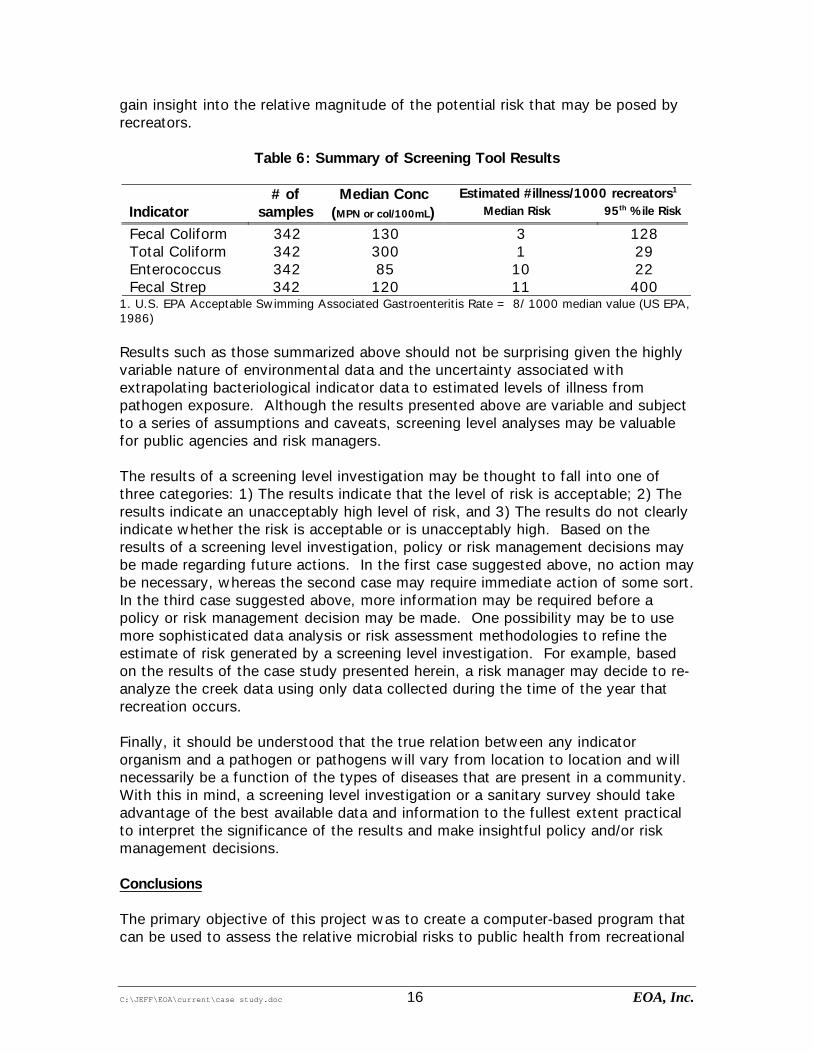
C:\JEFF\EOA\current\case study.doc 16 EOA, Inc.
gain insight into the relative magnitude of the potential risk that may be posed by recreators.
Table 6: Summary of Screening Tool Results
Median Conc Estimated #illness/1000 recreators1 Indicator
# of samples (MPN or col/100mL) Median Risk 95th %ile Risk
Fecal Coliform 342 130 3 128 Total Coliform 342 300 1 29 Enterococcus 342 85 10 22 Fecal Strep 342 120 11 400
1. U.S. EPA Acceptable Swimming Associated Gastroenteritis Rate = 8/ 1000 median value (US EPA, 1986) Results such as those summarized above should not be surprising given the highly variable nature of environmental data and the uncertainty associated with extrapolating bacteriological indicator data to estimated levels of illness from pathogen exposure. Although the results presented above are variable and subject to a series of assumptions and caveats, screening level analyses may be valuable for public agencies and risk managers. The results of a screening level investigation may be thought to fall into one of three categories: 1) The results indicate that the level of risk is acceptable; 2) The results indicate an unacceptably high level of risk, and 3) The results do not clearly indicate whether the risk is acceptable or is unacceptably high. Based on the results of a screening level investigation, policy or risk management decisions may be made regarding future actions. In the first case suggested above, no action may be necessary, whereas the second case may require immediate action of some sort. In the third case suggested above, more information may be required before a policy or risk management decision may be made. One possibility may be to use more sophisticated data analysis or risk assessment methodologies to refine the estimate of risk generated by a screening level investigation. For example, based on the results of the case study presented herein, a risk manager may decide to re-analyze the creek data using only data collected during the time of the year that recreation occurs. Finally, it should be understood that the true relation between any indicator organism and a pathogen or pathogens will vary from location to location and will necessarily be a function of the types of diseases that are present in a community. With this in mind, a screening level investigation or a sanitary survey should take advantage of the best available data and information to the fullest extent practical to interpret the significance of the results and make insightful policy and/or risk management decisions. Conclusions The primary objective of this project was to create a computer-based program that can be used to assess the relative microbial risks to public health from recreational
C:\JEFF\EOA\current\case study.doc 17 EOA, Inc.
exposure to urban creek waters. This memorandum illustrated the utility of the screening tool through a case study example. The results of the case study demonstrated that the estimated risk of infection from recreational exposure may vary from one indicator organism to the next. With respect to determining whether or not a beneficial use may be impaired due to exceedances of bacterial indicator data, the previous observation highlights the need to critically evaluate all available information related to those beneficial uses prior to attempting to make such an assessment. References Eisenberg, J.N., E.Y. Seto, A.W. Olivieri, R.C. Spear, "Quantifying Water Pathogen Risk in
an Epidemiological Framework", Society for Risk Analysis, pp.549-563, 1996. Eisenberg, J.N., E.Y. Seto, J.M. Colford, A.W. Olivieri, R.C. Spear, “An Analysis of the
Milwaukee Cryptosporidiosis Outbreak Based on a Dynamic Model of the Infection Process”, Epidemiology, 9: #3, May, 1998.
EOA, Inc, 1999. SCVURPPP Monitoring Project, Microbial Indicators and Effects on Beneficial Uses, Work Plan (Included as attachment to Soller and Olivieri, 2001).
RWQCB San Francisco Bay Basin Region, Water Quality Control Plan, 1995.
Soller, J. A. and A.W. Olivieri, 2001. Microbial Indicators and Effects on Beneficial Uses, Microbial Risk Screening Tool, Technical Memorandum Prepared by EOA, Inc. for the Santa Clara Valley Urban Runoff Pollution Prevention Program, 2001.
US EPA, 1986. Ambient Water Quality for Bacteria, EPA440/5-84-002, 1986.

C:\JEFF\EOA\current\case study.doc 18 EOA, Inc.
Appendix A: Summary of Assumptions Used to Generate Results for Enterococcus

C:\JEFF\EOA\current\case study.doc 19 EOA, Inc.
Assumptions of Water Risk EstimatorNotes:
1)The analysis carried out in this program is based on the assumption that an outlier analysis has been performed and that all data input are representative of the water body under study. Users should refer to textbooks on environmental data analysis for a thorough discussion on this topic. It should be understood that outliers will impact the results of the computations carried out in this program, and that data that are not considered representative should be removed prior to running this program.
2)This microbial risk screening tool estimates risk from exposure to waterborne pathogens from recreational contact based on the risk of viral infection. Adverse health effects from exposure to recreational waters may occur from exposure to bacteria, parasites, and/or viruses, all of which may be present when waters are fecally contaminated. A large base of literature, however suggests that the vast majority of the risk associated with recreational exposure to waterborne pathogens is from viral agents. Supporting evidence is available from the World Health Organization (1999) and from the CDC (Mead et al., 1999).
A. Raw Indicator Concentration Data (Bars) and Corresponding Maximum Likelihood Fit (Line)
On the initial screen, the user inputs Enterococcus concentration data and chooses the indicator organism (Enterococcus). These data are presented in Graph A as a histogram.
The line in Graph A represents the maximum likelihood fit of this data using either a lognormal or a weibull distribution. The distribution is selected based on skewness; a lognormal is selected if the data are positively skewed and a weibull is used if the data are negatively skewed (Ott, 1995).
B. Ingestion Rate Distribution
The distribution of ingestion amounts is assumed to be lognormal with a mean value of 50 ml per exposure event and 90% of ingestion events between 25 and 75 ml. (Roseberry and Burmaster, 1992).
C. Expected Dose of Pathogen
A dose is calculated by sampling once from the indicator concentration distribution and once from the ingestion rate distribution and then multiplying these two resulting values. This process is repeated 500 times yielding the dose (number organisms/event) histogram shown in Graph C.
D. Dose-Response Function
To calculate risk for Enterococcus, the following equation was used:
Y = -6.278 + 9.40 log (x)
where y is the illness rate per 1000 swimmers and x is the Enterococcus density per 100 ml (US EPA, 1986). This relationship is based on epidemiological studies carried at freshwater recreation areas by the US EPA.
E and F. Resultant Distribution of Risk
Risk (probability of infection per person per exposure event) is calculated by randomly sampling the concentration distribution shown in Graph A and plugging the result into the function shown in Graph D. This random sampling calculation is performed 500 times and the result is shown both as a histogram and as a cumulative distribution of risk in Figures E and F.
In graph E only, to enable the clearest display of the bulk of the data, only the 0 to 95th percentiles of data are shown. Thus, the end of the tail is truncated on the graph. Graph F shows 100 percent of the data.

C:\JEFF\EOA\current\case study.doc 20 EOA, Inc.
G. Uncertainty of Risk
Uncertainty bounds for the risk estimate are calculated by varying the four parameters of the distributions in Graphs A and D and finding the 5th and 95th percentiles about the distribution in Graph E. The parameters varied are the two parameters describing the maximum likelihood fit of the raw data and the two parameters describing the shape of the dose response function.
Thus, in Graph G, the fifth and ninety-fifth percentile probabilities are plotted along with the maximum likelihood risk distribution from E.
H. References
United States Environmental Protection Agency, 1986. EPA 440/5-84-002, "Ambient Water Quality Criteria for Bacteria".
Ott W.R., "Environmental Statistics and Data Analysis", Lewis Publishers, Boca Raton, FL, 1995.
Roseberry, A. M. and D. E. Burmaster, 1992. "Log-normal Distributions for Water Intake by Children and Adults". Risk Analysis, 12 (1): 99-104.
Mead et al., 1999. Food-Related Illness and Death in the United States, Emerging Infectious Diseases, V.5 No.5.
World Health Organization, 1999. Health Based Monitoring of Recreational Waters: The Feasibility of a New Approach, WHO/SDE/WSH/99.1

C:\JEFF\EOA\current\case study.doc 21 EOA, Inc.
Appendix B: Summary of Assumptions Used to Generate Results for Fecal Coliform

C:\JEFF\EOA\current\case study.doc 22 EOA, Inc.
Assumptions of Water Risk EstimatorNotes:
1)The analysis carried out in this program is based on the assumption that an outlier analysis has been performed and that all data input are representative of the water body under study. Users should refer to textbooks on environmental data analysis for a thorough discussion on this topic. It should be understood that outliers will impact the results of the computations carried out in this program, and that data that are not considered representative should be removed prior to running this program.
2)This microbial risk screening tool estimates risk from exposure to waterborne pathogens from recreational contact based on the risk of viral infection. Adverse health effects from exposure to recreational waters may occur from exposure to bacteria, parasites, and/or viruses, all of which may be present when waters are fecally contaminated. A large base of literature, however suggests that the vast majority of the risk associated with recreational exposure to waterborne pathogens is from viral agents. Supporting evidence is available from the World Health Organization (1999) and from the CDC (Mead et al., 1999).
A. Raw Indicator Concentration Data (Bars) and Corresponding Maximum Likelihood Fit (Line)
On the initial screen, the user inputs fecal coliform concentration data and chooses the indicator organism (Fecal Coliform). These data are presented in Graph A as a histogram.
The line in Graph A represents the maximum likelihood fit of this data using either a lognormal or a weibull distribution. The distribution is selected based on skewness; a lognormal is selected if the data are positively skewed and a weibull is used if the data are negatively skewed (Ott, 1995).
This indicator data needs to be converted to pathogen concentration data in order to enable its use later in the dose response equation. The following equation converts Fecal Coliform concentration to enteric virus concentration:
Log(y) = -1.16 + 1.56 * Log(x)
where x is the concentration of Fecal Coliform (per mL) and y is the concentration of enteric viruses (per L). This relationship is based on a study by Havelaar et al. (1993). This relationship is applicable in river water. Although this relation may vary from site to site, it is currently the best available relationship.
Thus, a distribution for enteric virus concentration is constructed using this transformation. This new distribution is not shown in any of the Graphs A through F, but is used in calculating dose as described below.
B. Ingestion Rate Distribution
The distribution of ingestion amounts is assumed to be lognormal with a mean value of 50 ml per exposure event and 90% of ingestion events between 25 and 75 ml. (Roseberry and Burmaster, 1992).
C. Expected Dose of Pathogen
A dose is calculated by sampling once from the pathogen concentration distribution (converted from indicator concentrations) and once from the ingestion rate distribution and then multiplying these two resulting values. This process is repeated 500 times yielding the dose (number organisms/event) histogram shown in Graph C.
In order to clearly display most of the data, only the 0 to 95th percentiles of data are shown in graph C. Thus, the end of the tail is truncated on the graph.
D. Dose-Response Function
To calculate the probability of infection per person per exposure event for fecal coliform, the following dose-response function is used:
r = 1 - (1 + y / b)^(-a)
where r is the risk of infection, y is the predicted dose, and a and b are the parameters corresponding to 0.26 and 0.42. This relationship between enteric virus and risk of infection is based on a maximum likelihood fit of data obtained from a rotavirus dosing trial (Ward et al. 1986) using a beta Poisson function (Hass, 1983).
E and F. Resultant Distribution of Risk
Risk (probability of infection per person per exposure event) is calculated by randomly sampling the enteric virus dose distribution shown in Graph C and plugging the result into the dose-response function shown in D. This random sampling calculation is performed 500 times and the result is shown both as a histogram and as a cumulative distribution of risk in Figures E and F.
In graph E only, to enable the clearest display of the bulk of the data, only the 0 to 95th percentiles of data are shown. Thus, the end of the tail is truncated on the graph. Graph F shows 100 percent of the data.

C:\JEFF\EOA\current\case study.doc 23 EOA, Inc.
G. Uncertainty of Risk
Uncertainty bounds for the risk estimate are calculated by varying the six parameters of the distributions in Graphs A, C, and D and finding the 5th and 95th percentiles about the distribution in Graph E. The parameters varied are the two parameters describing the maximum likelihood fit of the raw data, the two parameters describing the shape of the dose response function, and the two parameters describing the relation between indicator and pathogen concentration.
Thus, in Graph G, the fifth and ninety-fifth percentile probabilities are plotted along with the maximum likelihood risk distribution from E.
H. References
United States Environmental Protection Agency, 1986. EPA 440/5-84-002, "Ambient Water Quality Criteria for Bacteria".
Haas, C. N., 1983. "Estimation of Risk Due to Low Doses of Microorganisms: a Comparison of Alternative Methodologies". American Journal of Epidemiology, 118 (4): 573-82.
Havelaar, A.H., M. Van Olphen, and Y.C. Drost, 1993. F-specific bacteriophages are adequate model organisms for enteric viruses in fresh water. Applied & Environmental Microbiology, pp.2956-62.
Ott W.R., "Environmental Statistics and Data Analysis", Lewis Publishers, Boca Raton, FL, 1995.
Roseberry, A. M. and D. E. Burmaster, 1992. "Log-normal Distributions for Water Intake by Children and Adults". Risk Analysis, 12 (1): 99-104.
Ward, R. L., D. I. Bernstein, E. C. Young, J. R. Sherwood, D. R. Knowlton and G. M. Schiff, "Human Rotavirus Studies in Volunteers: Determination of Infectious Dose and Serological Response to Infection," Journal of Infectious Disease, 154, 871-880, 1986.
Mead et al., 1999. Food-Related Illness and Death in the United States, Emerging Infectious Diseases, V.5 No.5.
World Health Organization, 1999. Health Based Monitoring of Recreational Waters: The Feasibility of a New Approach, WHO/SDE/WSH/99.1

C:\JEFF\EOA\current\case study.doc 24 EOA, Inc.
Appendix C: Summary of Assumptions Used to Generate Results for Total Coliform

C:\JEFF\EOA\current\case study.doc 25 EOA, Inc.
Assumptions of Water Risk EstimatorNotes:
1)The analysis carried out in this program is based on the assumption that an outlier analysis has been performed and that all data input are representative of the water body under study. Users should refer to textbooks on environmental data analysis for a thorough discussion on this topic. It should be understood that outliers will impact the results of the computations carried out in this program, and that data that are not considered representative should be removed prior to running this program.
2)This microbial risk screening tool estimates risk from exposure to waterborne pathogens from recreational contact based on the risk of viral infection. Adverse health effects from exposure to recreational waters may occur from exposure to bacteria, parasites, and/or viruses, all of which may be present when waters are fecally contaminated. A large base of literature, however suggests that the vast majority of the risk associated with recreational exposure to waterborne pathogens is from viral agents. Supporting evidence is available from the World Health Organization (1999) and from the CDC (Mead et al., 1999).
A. Raw Indicator Concentration Data (Bars) and Corresponding Maximum Likelihood Fit (Line)
On the initial screen, the user inputs raw total Coliform concentration data and chooses the indicator organism (Total Coliform). These data are presented in Graph A as a histogram.
The line in Graph A represents the maximum likelihood fit of this data using either a lognormal or a weibull distribution. The distribution is selected based on skewness; a lognormal is selected if the data are positively skewed and a weibull is used if the data are negatively skewed (Ott, 1995).
This indicator data needs to be converted to pathogen concentration data in order to enable its use later in the dose response equation. Total coliform is first converted to fecal coliform either using a percentage input by the user or by using a default relationship developed by the United States Environmental Protection Agency (US EPA, 1986). In this relationship, Fecal Coliform concentrations are assumed to be 18% of the Total Coliform concentrations.
The following equation converts fecal coliform concentration to enteric virus concentration:
Log(y) = -1.16 + 1.56 * Log(x)
where x is the concentration of fecal coliform (per mL) and y is the concentration of enteric viruses (per L). This relationship is based on a study by Havelaar et al. (1993). It applies in river water and coagulated secondary effluent, and though it may vary from site to site, it is currently the best available relationship.
Thus, a distribution for enteric virus concentration is constructed using these two transformations. This new distribution is not shown in any of the Graphs A through F, but is used in calculating dose as described below.
B. Ingestion Rate Distribution
The distribution of ingestion amounts is assumed to be lognormal with a mean value of 50 ml per exposure event and 90% of ingestion events between 25 and 75 ml. (Roseberry and Burmaster, 1992).
C. Expected Dose of Pathogen
A dose is calculated by sampling once from the pathogen concentration distribution (converted from indicator concentrations) and once from the ingestion rate distribution and then multiplying these two resulting values. This process is repeated 500 times yielding the dose (number organisms/event) histogram shown in Graph C.
In order to clearly display most of the data, only the 0 to 95th percentiles of data are shown in graph C. Thus, the end of the tail is truncated on the graph.
D. Dose-Response Function
To calculate the probability of infection per person per exposure event for total coliform, the following dose-response function is used:
r = 1 - (1 + y / b)^(-a)
where r is the risk of infection, y is the predicted dose, and a and b are the parameters corresponding to 0.26 and 0.42. This relationship between enteric virus and risk of infection is based on a maximum likelihood fit of data obtained from a rotavirus dosing trial (Ward et al. 1986) using a beta Poisson function (Hass, 1983).
E and F. Resultant Distribution of Risk
Risk (probability of infection per person per exposure event) is calculated by randomly sampling the enteric virus dose distribution shown in Graph C and plugging the result into the dose-response function shown in D. This random sampling calculation is performed 500 times and the result is shown both as a histogram and as a cumulative distribution of risk in Figures E and F.
In graph E only, to enable the clearest display of the bulk of the data, only the 0 to 95th percentiles of data are shown. Thus, the end of the tail is truncated on the graph. Graph F shows 100 percent of the data.

C:\JEFF\EOA\current\case study.doc 26 EOA, Inc.
G. Uncertainty of Risk
Uncertainty bounds for the risk estimate are calculated by varying the six parameters of the distributions in Graphs A, C, and D and finding the 5th and 95th percentiles about the distribution in Graph E. The parameters varied are the two parameters describing the maximum likelihood fit of the raw data, the two parameters describing the shape of the dose response function, and the two parameters describing the relation between indicator and pathogen concentration.
Thus, in Graph G, the fifth and ninety-fifth percentile probabilities are plotted along with the maximum likelihood risk distribution from E.
H. References
United States Environmental Protection Agency, 1986. EPA 440/5-84-002, "Ambient Water Quality Criteria for Bacteria".
Haas, C. N., 1983. "Estimation of Risk Due to Low Doses of Microorganisms: a Comparison of Alternative Methodologies". American Journal of Epidemiology, 118 (4): 573-82.
Havelaar, A.H., M. Van Olphen, and Y.C. Drost, 1993. F-specific bacteriophages are adequate model organisms for enteric viruses in fresh water. Applied & Environmental Microbiology, pp.2956-62.
Ott W.R., "Environmental Statistics and Data Analysis", Lewis Publishers, Boca Raton, FL, 1995.
Roseberry, A. M. and D. E. Burmaster, 1992. "Log-normal Distributions for Water Intake by Children and Adults". Risk Analysis, 12 (1): 99-104.
Ward, R. L., D. I. Bernstein, E. C. Young, J. R. Sherwood, D. R. Knowlton and G. M. Schiff, "Human Rotavirus Studies in Volunteers: Determination of Infectious Dose and Serological Response to Infection," Journal of Infectious Disease, 154, 871-880, 1986.
Mead et al., 1999. Food-Related Illness and Death in the United States, Emerging Infectious Diseases, V.5 No.5.
World Health Organization, 1999. Health Based Monitoring of Recreational Waters: The Feasibility of a New Approach, WHO/SDE/WSH/99.1

C:\JEFF\EOA\current\case study.doc 27 EOA, Inc.
Appendix D: Summary of Assumptions Used to Generate Results for Fecal
Streptococcus

C:\JEFF\EOA\current\case study.doc 28 EOA, Inc.
Assumptions of Water Risk EstimatorNotes:
1)The analysis carried out in this program is based on the assumption that an outlier analysis has been performed and that all data input are representative of the water body under study. Users should refer to textbooks on environmental data analysis for a thorough discussion on this topic. It should be understood that outliers will impact the results of the computations carried out in this program, and that data that are not considered representative should be removed prior to running this program.
2)This microbial risk screening tool estimates risk from exposure to waterborne pathogens from recreational contact based on the risk of viral infection. Adverse health effects from exposure to recreational waters may occur from exposure to bacteria, parasites, and/or viruses, all of which may be present when waters are fecally contaminated. A large base of literature, however suggests that the vast majority of the risk associated with recreational exposure to waterborne pathogens is from viral agents. Supporting evidence is available from the World Health Organization (1999) and from the CDC (Mead et al., 1999).
A. Raw Indicator Concentration Data (Bars) and Corresponding Maximum Likelihood Fit (Line)
On the initial screen, the user inputs fecal streptococcus concentration data and chooses the indicator organism (Fecal Streptococcus). These data are presented in Graph A as a histogram.
The line in Graph A represents the maximum likelihood fit of this data using either a lognormal or a weibull distribution. The distribution is selected based on skewness; a lognormal is selected if the data are positively skewed and a weibull is used if the data are negatively skewed (Ott, 1995).
This indicator data needs to be converted to pathogen concentration data in order to enable its use later in the dose response equation. The following equation converts Fecal Streptococcus concentrations to enteric virus concentration:
Log(y) = -0.2 + 1.81 * Log(x)
where x is the concentration of Fecal Streptococcus (per mL) and y is the concentration of enteric viruses (per L). This relationship is based on a study by Havelaar et al. (1993). Though it may vary from site to site, it is currently the best available relationship.
Thus, a distribution for enteric virus concentration is constructed using this transformation. This new distribution is not shown in any of the Graphs A through F, but is used in calculating dose as described below.
B. Ingestion Rate Distribution
The distribution of ingestion amounts is assumed to be lognormal with a mean value of 50 ml per exposure event and 90% of ingestion events between 25 and 75 ml. (Roseberry and Burmaster, 1992).
C. Expected Dose of Pathogen
A dose is calculated by sampling once from the pathogen concentration distribution (converted from indicator concentrations) and once from the ingestion rate distribution and then multiplying these two resulting values. This process is repeated 500 times yielding the dose (number organisms/event) histogram shown in Graph C.
In order to clearly display most of the data, only the 0 to 95th percentiles of data are shown in graph C. Thus, the end of the tail is truncated on the graph.
D. Dose-Response Function
To calculate the probability of infection per person per exposure event for fecal streptococcus, the following dose-response function is used:
r = 1 - (1 + y / b)^(-a)
where r is the risk of infection, y is the predicted dose, and a and b are the parameters corresponding to 0.26 and 0.42. This relationship between enteric virus and risk of infection is based on a maximum likelihood fit of data obtained from a rotavirus dosing trial (Ward et al. 1986) using a beta Poisson function (Hass, 1983).
E and F. Resultant Distribution of Risk
Risk (probability of infection per person per exposure event) is calculated by randomly sampling the enteric virus dose distribution shown in Graph C and plugging the result into the dose-response function shown in D. This random sampling calculation is performed 500 times and the result is shown both as a histogram and as a cumulative distribution of risk in Figures E and F.
In graph E only, to enable the clearest display of the bulk of the data, only the 0 to 95th percentiles of data are shown. Thus, the end of the tail is truncated on the graph. Graph F shows 100 percent of the data.

C:\JEFF\EOA\current\case study.doc 29 EOA, Inc.
G. Uncertainty of Risk
Uncertainty bounds for the risk estimate are calculated by varying the six parameters of the distributions in Graphs A, C, and D and finding the 5th and 95th percentiles about the distribution in Graph E. The parameters varied are the two parameters describing the maximum likelihood fit of the raw data, the two parameters describing the shape of the dose response function, and the two parameters describing the relation between indicator and pathogen concentration.
Thus, in Graph G, the fifth and ninety-fifth percentile probabilities are plotted along with the maximum likelihood risk distribution from E.
H. References
United States Environmental Protection Agency, 1986. EPA 440/5-84-002, "Ambient Water Quality Criteria for Bacteria".
Haas, C. N., 1983. "Estimation of Risk Due to Low Doses of Microorganisms: a Comparison of Alternative Methodologies". American Journal of Epidemiology, 118 (4): 573-82.
Havelaar, A.H., M. Van Olphen, and Y.C. Drost, 1993. F-specific bacteriophages are adequate model organisms for enteric viruses in fresh water. Applied & Environmental Microbiology, pp.2956-62.
Ott W.R., "Environmental Statistics and Data Analysis", Lewis Publishers, Boca Raton, FL, 1995.
Roseberry, A. M. and D. E. Burmaster, 1992. "Log-normal Distributions for Water Intake by Children and Adults". Risk Analysis, 12 (1): 99-104.
Ward, R. L., D. I. Bernstein, E. C. Young, J. R. Sherwood, D. R. Knowlton and G. M. Schiff, "Human Rotavirus Studies in Volunteers: Determination of Infectious Dose and Serological Response to Infection," Journal of Infectious Disease, 154, 871-880, 1986.
Mead et al., 1999. Food-Related Illness and Death in the United States, Emerging Infectious Diseases, V.5 No.5.
World Health Organization, 1999. Health Based Monitoring of Recreational Waters: The Feasibility of a New Approach, WHO/SDE/WSH/99.1