emva standard 1288 · jai/pulnix tue moerk ... all pixels start exposing and stop exposing at the...

September 06 Copyright EMVA, 2005

EMVA Standard 1288 Standard for Characterization and Presentation of Speci-fication Data for Image Sensors and Cameras Release A1.03

Standard for Characterization and Presentation of Specification Data for Image Sensors and Cameras

September 06 Release A1.03

of 23 Copyright EMVA, 2005

Acknowledgements

Companies participate in the elaboration of the EMVA Standard 1288 and they're representatives

Company Represented by:

Adimec Jochem Herrmann

Asentics Wolfgang Pomrehn

Aspect Systems Marcus Verhoeven

ATMEL Jacques Leconte

AWAIBA Martin Wäny

Basler Dr. Friedrich Dierks

DALSA Prof. Dr. Albert Theuwissen

BOSCH Dr. Uve Apel

IDT Daniel Diezemann

JAI/Pulnix Tue Moerk

MELEXIS Dr. Arnaud Darmont

PCO Dr. Gerhard Holst

Sony Jérôme Avenel

Stemmer Imaging Martin Kersting / Manfred Wütschner

TVI Vision Kari Siren / Jari Löytömaki

University Heidelberg Prof. Dr. Bernd Jähne

University Oldenburg Dr. Heinz Helmers

Rights and Trademarks

The European Machine Vision Association owns the "EMVA, standard 1288 compliant" logo. Any com-pany can obtain a license to use the "EMVA standard 1288 compliant" logo, free of charge, with prod-uct specifications measured and presented according to the definitions in EMVA standard 1288. The licensee guarantees that he meets the terms of use in the relevant version of EMVA standard 1288. Licensed users will self -certify compliance of their measurement setup, computation and represent a-tion with which the "EMVA standard 1288 compliant" logo is used. The licensee has to check reg ularly compliance with the relevant version of EMVA standard 1288, at least once a year. When di splayed on line the logo has to be featured with a link to EMVA standardization web page. EMVA will not be liable for specifications not compliant with the standard and damage r esulting there from. EMVA keeps the right to withdraw the granted license any time and without giving reasons.




About this Standard EMVA has started the initiative to define a unified method to measure, compute and present specifica-tion parameters and characterization data for cameras and image sensors used for machine vision applications.

The standard does not define what nature of data should be disclosed. It is up to the component manufacturer to decide if he wishes to publish typical data, data of an individual component, guaran-teed data, or even guaranteed performance over life time of the component. However the component manufacturer shall clearly indicate what the nature of the presented data is.

The Standard is organized in different modules, each addressing a group of specification parameters, assuming a certain physical behavior of the sensor or camera under c ertain boundary conditions. Ad-ditional modules covering more parameters and a wider range of sensor and camera products will be added at a later date.

For the time being it will be necessary for the manufacturer to indicate additional, component specific information, not defined in the standard, to fully describe the performance of image sensor or camera products, or to describe physical behavior not covered by the mathematical mo dels of the standard.

The purpose of the standard is to benefit the Automated Vision Industry by providing fast, comprehen-sive and consistent access to specification information for Cameras and Sensors. Particularly it will be beneficial for those who wish to compare cameras or who wish to calculate system performance based on the performance specifications of a image sensor or a camera.




Contents

ACKNOWLEDGEMENTS 2

RIGHTS AND TRADEMARK S 2

ABOUT THIS STANDARD 3

CONTENTS 4

4 INTRODUCTION AND SCOPE 5

5 BASIC INFORMATION 6

6 GENERAL DEFINITIONS 7

6.1 ACTIVE AREA 7 6.2 NUMBER OF PIXELS 7 6.3 (GEOMETRICAL) PIXEL AREA 7

7 MODULE 1: CHARACTERIZING THE IMAGE QUALITY AND SENSITIVITY OF MACHINE VISION CAMERAS AND SENSORS 8

7.1 MATHEMATICAL MODEL 8 7.2 MEASUREMENT SETUP 12 7.3 MATCHING THE MODEL TO THE DATA 13 7.3.1 EXTENDED PHOTON TRANSFER METHOD 13 7.3.2 SPECTROGRAM METHOD 16 7.4 PUBLISHING THE RESULTS 20 7.4.1 CHARACTERIZING TEMPORAL NOISE AND SENSITIVITY 20 7.4.2 CHARACTERIZING TOTAL AND SPATIAL NOISE 21

8 REFERENCES 23




4 Introduction and Scope The first version of this standard covers monochrome digital area scan cameras with linear photo re-sponse characteristics. Line scan and color cameras will follow.

Analog cameras can be described according to this standard in conjunction with a frame grabber; similarly, image sensors can be described as part of a camera.

The standard text is organized into separate modules. The first module covers noise and sensitivity. More modules will follow in future versions of the standard.

Camera

Mathematical Model

Parameters

Matching themodel to the

data

Measurementdata

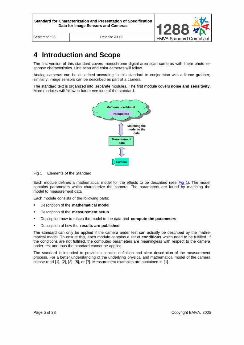
Fig 1 Elements of the Standard

Each module defines a mathematical model for the effects to be described (see Fig 1). The model contains parameters which characterize the camera. The parameters are found by matching the model to measurement data.

Each module consists of the following parts:

§ Description of the mathematical model

§ Description of the measurement setup

§ Description how to match the model to the data and compute the parameters

§ Description of how the results are published

The standard can only be applied if the camera under test can actually be described by the mathe-matical model. To ensure this, each module contains a set of conditions which need to be fulfilled. If the conditions are not fulfilled, the computed parameters are meaningless with respect to the camera under test and thus the standard cannot be applied.

The standard is intended to provide a concise definition and clear description of the measurement process. For a better understanding of the underlying physical and mathematical model of the camera please read [1], [2], [3], [5], or [7]. Measurement examples are contained in [1].




5 Basic Information Before discussing the modules, this section describes the basic information which must be published for each camera:

§ Vendor name

§ Model name

§ Type of data presented: Typical; Guaranteed; Guaranteed over life time 1

§ Sensor type

CCD; CMOS; CID etc...

§ Sensor diagonal in [mm] (Sensor length in the case of line sensors)

§ Indication of lens category to be used [inch]

§ Resolution of the sensor’s active area (width x height in [pixels])

§ Pixel size (width x height in [µm])

§ Readout type (CCD only)

− progressive scan

− interlaced

§ Transfer type (CCD only)

− Interline transfer

− Frame transfer

− Full frame transfer

− Frame interline transfer

−

§ Shutter type (CMOS only)

− Global : all pixels start exposing and stop exposing at the same time.

− Rolling : exposure starts line by line with a slight delay between line starts; the exposure time for each line is the same.

− Others : defined in the data-sheet.

§ Overlap capabilities

− Overlapping : readout of frame n and exposure of frame n+1 can happen at the same time.

− Non-overlapping : readout of frame n and exposure of frame n+1 can only happen sequen-tially.

− Others : defined in the data-sheet.

§ Maximum frame rate at the given operation point. (no change of settings permi tted)

§ General conventions

§ Definition used for typical data. (Number of samples, sample selection) .

§ Others (Interface Type etc.)

1 The type of data may vary for different parameters. E.g. guaranteed specification for most of the parameters and typical data for some measurements not easily done in production (e.g. η(λ)). It then has to be clearly indicated which data is of what nature.




6 General definitions This section defines general terms used in the different modules

6.1 Active Area The Active Area of an image sensor or of a camera is defined as the array of light sensitive pi xels that are functional2 in normal operation mode.

6.2 Number of Pixels The number of pixels is defined as: The number of pixels is the number of separate, physically existing and light sensitive photosites in the Active Area3. Stacked photosites4 are counted as a single pixel The number of pixels of a sensor / camera is indicated in number of column s x number of rows. (E.g. 640 x 480)

6.3 (Geometrical) Pixel Area

Geometrical not necessarily light sensitive area of a pixel, given by horizontal pixel pitch x vertical pixel pitch.

2 Functional in this context means that the pixel values are given out. 3 Dark pixels are not counted 4 Stacked pixels are sometimes used for colour separation




7 Module 1: Characterizing the Image Quality and Sensitivity of Machine Vision Cameras and Sen-sors

This module describes how to characterize the temporal and spatial noise of a camera and its sensitiv-ity to light.

7.1 Mathematical Model

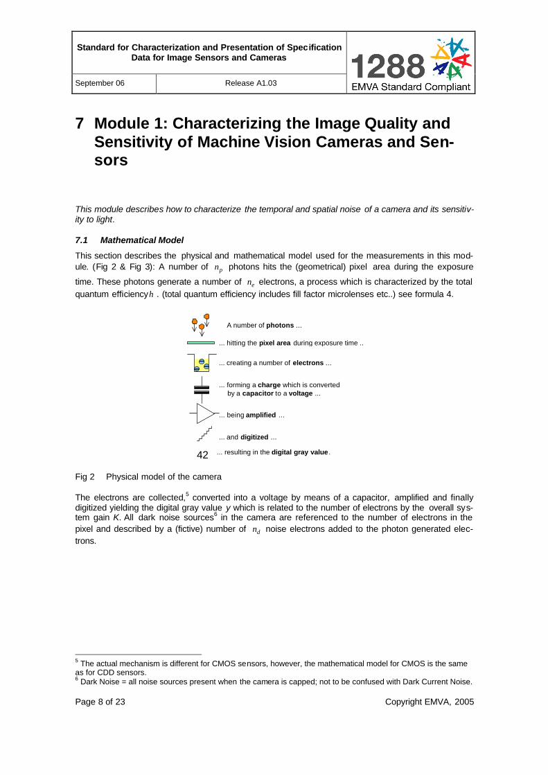
This section describes the physical and mathematical model used for the measurements in this mod-ule. (Fig 2 & Fig 3): A number of pn photons hits the (geometrical) pixel area during the exposure

time. These photons generate a number of en electrons, a process which is characterized by the total quantum efficiencyη . (total quantum efficiency includes fill factor microlenses etc..) see formula 4.

42

A number of photons ...

... hitting the pixel area during exposure time ...

... creating a number of electrons ...

... forming a charge which is converted by a capacitor to a voltage ...

... being amplified ...

... and digitized ...

... resulting in the digital gray value .

Fig 2 Physical model of the camera

The electrons are collected,5 converted into a voltage by means of a capacitor, amplified and finally digitized yielding the digital gray value y which is related to the number of electrons by the overall sys-tem gain K. All dark noise sources6 in the camera are referenced to the number of electrons in the pixel and described by a (fictive) number of dn noise electrons added to the photon generated elec-trons.

5 The actual mechanism is different for CMOS sensors, however, the mathematical model for CMOS is the same as for CDD sensors. 6 Dark Noise = all noise sources present when the camera is capped; not to be confused with Dark Current Noise.




pe

K yηnn

dnquantumefficiency

system gain

number ofphotons

number ofelectrons

digital grey value

dark noise

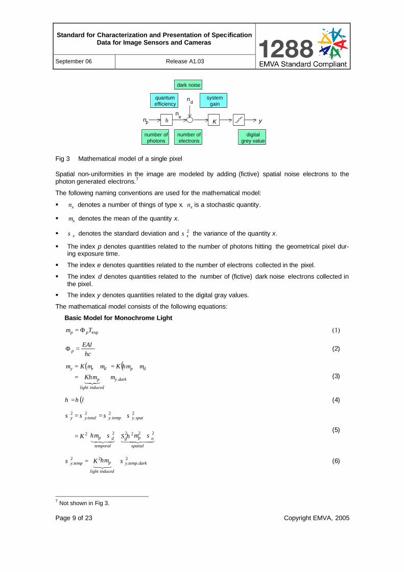
Fig 3 Mathematical model of a single pixel

Spatial non-uniformities in the image are modeled by adding (fictive) spatial noise electrons to the photon generated electrons.7

The following naming conventions are used for the mathematical model:

§ xn denotes a number of things of type x. xn is a stochastic quantity.

§ xµ denotes the mean of the quantity x.

§ xσ denotes the standard deviation and 2xσ the variance of the quantity x.

§ The index p denotes quantities related to the number of photons hitting the geometrical pixel dur-ing exposure time.

§ The index e denotes quantities related to the number of electrons collected in the pixel.

§ The index d denotes quantities related to the number of (fictive) dark noise electrons collected in the pixel.

§ The index y denotes quantities related to the digital gray values.

The mathematical model consists of the following equations:

Basic Model for Monochrome Light

expTpp Φ=µ (1)

hcEA

pλ=Φ (2)

( ) ( )darky

inducedlight

p

dpdey

K

KK

.µηµ

µηµµµµ

+=

+=+=

321 (3)

( )ληη = (4)

+++=

+==

44 3442143421spatial

opg

temporal

dp

spatytempytotalyy

SK 222222

2.

2.

2.

2

σµησηµ

σσσσ

(5)

2..

22. darktempy

inducedlight

ptempy K σηµσ +=321

(6)

7 Not shown in Fig 3.




2..

22222. darkspaty

inducedlight

pgspaty SK σµησ +=43421

(7)

Saturation

satysaturationy .µµ → . (8)

02 →saturationyσ (9)

satpdsatpsate ... ηµµηµµ ≈+= (10)

Model Extension for Dark Current Noise

expd0d TNd+= µµ (11)

exp2

02 TNddd += σσ (12)

dkC

dd NN°−

=30

30 2ϑ

(13)

Model Extension for Non-White Noise

2.

2.

2. nonwhiteywhiteyfully σσσ += (14)

Derived Measures

( ) 222220 pgpod

py

SSNR

µηηµσσ

ηµ

+++= (15)

ησ

µ 0min.

dp = (16)

min.

.

p

satpinDYN

µ

µ= (see footnotes89) (17)

0

.

d

sateoutDYN

σµ

= (18)

2.

2.

whitey

fullyFσ

σ= (19)

Alternative Measures10

gSPRNU =1288 (20)

oDSNU σ=1288 (21)

8 For linear sensors, outin DYNDYN = holds true. 9 The dynamic range must be present in the same image (“intra scene”). 10 These measures are given for convenience. Note that for historical reasons several inconsistent definitions of these terms exist. Therefore the 1288 suffix should always be used.




using the following quantities with their units given in square brackets:

A area of the (geometrical) pixel [m2]

c Speed of light sm

103 8⋅≈c

inDYN Input dynamic range [1]

outDYN Output dynamic range [1] E irradiance on the sensor surface [W/m2] F Non-whiteness coefficient h Planck’s constant Js1063.6 34−≈h

K overall system gain [DN/e-]

dk Doubling temperature of the dark current [°C]

dN dark current [e-/s]

30dN dark current for a housing temperature of 30°C [e-/s] 2gS variance coefficient of the spatial gain noise [%2]

PRNU1288 photo response non-uniformity [%] ySNR gray value’s signal-to-noise ratio [%]

expT exposure time [s]

η total quantum efficiency11 [e-/p~] = [1] = [%] ϑ housing temperature of the camera [°C] λ wavelength of light [m]

eµ mean number of photon generated electrons [e-]12

sate.µ saturation capacity, i.e. mean equivalent electrons if the camera is saturated [e-]

dµ mean number of (fictive) temporal dark noise electrons [e-]

0dµ mean number of (fictive) dark noise electrons for exposure time zero [e-]

pµ mean number of photons collected by one pixel during exposure time [p~] 13

min.pµ Absolute sensitivity threshold [p~]

satp.µ mean number of photons colleted if the camera is saturated [p~]

yµ mean gray value [DN] 14

darky.µ mean gray value with no light applied [DN]

saty.µ mean gray value if the camera is saturated [DN] 2dσ variance of temporal distribution of dark signal referred to electrons [e-2] 2

0dσ variance of the (fictive) temporal dark noise electrons for exposure time zero [e-2] 2oσ variance of the spatial offset noise [e-2]

DSNU1288 dark signal non-uniformity [e-] 2. fullyσ variance of the gray values’ distribution including white noise and artifacts [DN2]

2.nonwhiteyσ variance of the gray values’ distribution including the non-white part of the noise only [DN2]

2.spatyσ variance of spatial distribution of gray values (spatial noise) [DN2]

2.. darkspatyσ variance of the spatial distribution of dark signal (spatial dark noise) [DN2]

2.tempyσ variance of temporal distribution of gray values (temporal noise) [DN2]

11 Including the geometrical fill factor. 12 The unit [e-] = [e-2] = 1 denotes a number of electrons. 13 The unit [p~] = [p~2] = 1 denotes a number of photons. 14 The unit [DN] = [DN2] = 1 denotes digital numbers.




2.. darktempyσ variance of temporal distribution of dark signal (temporal dark noise) [DN2]

2.totalyσ variance of the distribution of gray values (total noise) [DN2]

2.whiteyσ variance of the gray values’ distribution including the white part of the noise only [DN2]

pΦ number of photons collected in the geometric pixel per unit exposure time [p~/s]

Throughout this document noise energy is described in terms of variance. An equivalent way would be using rms (root mean square) values. The following relation holds true: variance = rms2.

The model contains several important assumptions that need to be challenged during the qualification:

§ The amount of photons collected by a pixel depends on the product of irradiance and exposure time.

§ All noise sources are stationary and white with respect to time and space.15 The parameters de-scribing the noise are invariant with respect to time and space.

§ Only the total quantum efficiency is wavelength dependent. The effects caused by light of different wavelengths can be linearly superimposed.

§ Only the dark current is temperature dependent.

If these assumptions do not hold true and the mathematical model cannot be matched to the meas-urement data, the camera cannot be characterized using this standard.

7.2 Measurement Setup

The measurements described in the following section use dark and bright measurements. Dark meas-urements are performed while the camera is capped.

Bright measurements are taken without a lens and in a dark room. The sensor is illuminated by a dif-fuse disk-shaped light source16 placed in front of the camera (see Fig. 4). Each pixel must “see” the whole disk.17 No reflection shall take place.18

Fig. 4 : Optical setup

The f-number of this setup is defined as:

Dd

f =# (22)

15 The spectrogram method (see section 7.3.2) is used to challenge this assumption. 16 This could be, for example, the port of an a Ulbricht sphere. A good diffuser with circular ape rture would also do. 17 Beware, the mount forms an artificial horizon for the pixels and might occlude parts of the disk for pixels located at the border of the sensor. 18 Especially not on the mount's inside screw thread.

sensor

disk

-sha

ped

light

sou

rce

mount

d

D D'

temperature sensor




with the following quantities: d distance from sensor to light source [m] D diameter of the disk-shaped light source [m]

The f-number must be 8.

If not otherwise stated, measurements are performed at a 30°C camera housing temperature. The housing temperature is measured by placing a temperature sensor at the lens mount. For cameras consuming a lot of power, measurements may be performed at a higher temperature.

Measurements are done with monochrome light. Use of the wavelength where the quantum efficiency of the camera under test is maximal is recommended. The wavelength variation must be nm50≤ .

The amount of light falling on the sensor is measured with an accuracy19 of better than ±5%. The char-acteristic of non-removable filters is taken as part of the camera characteristic.

The number of photons hitting the pixel during exposure time is varied by changing the exposure time and computed using equations (1) and (2).

All camera settings (besides the variation of exposure time where stated) are identical for all meas-urements. For different settings (e.g., gain) different sets of measurements must be acquired and dif-ferent sets of parameters, containing all parameters20 which may influence the characteristic of the camera, must be presented.

7.3 Matching the Model to the Data

7.3.1 Extended Photon Transfer Method

The measurement scheme described in this section is based on the “Photon Transfer Method” (see [4]) and identifies those model parameters which deal with temporal noise.

For a fixed set of camera settings, two series of measurements are performed with varying exposure times21 expT :

§ First a dark run is performed and the following quantities are determined (details below): expT , darky.µ , and 2

.. darktempyσ .

§ Second a bright run is performed and the following quantities are determined: expT , pµ , yµ , and 2.tempyσ .

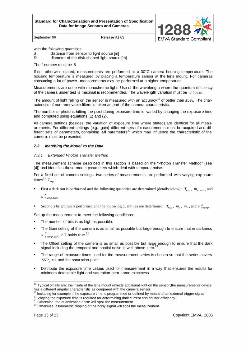
Set up the measurement to meet the following conditions:

§ The number of bits is as high as possible.

§ The Gain setting of the camera is as small as possible but large enough to ensure that in darkness

12.. ≥darktempyσ holds true.22

§ The Offset setting of the camera is as small as possible but large enough to ensure that the dark signal including the temporal and spatial noise is well above zero.23

§ The range of exposure times used for the measurement series is chosen so that the series covers 1=ySNR and the saturation point.

§ Distribute the exposure time values used for measurement in a way that ensures the results for minimum detectable light and saturation bear same exactness.

19 Typical pitfalls are: the inside of the lens mount reflects additional light on the sensor ;the measurements device has a different angular characteristic as compared with the came ra sensor. 20 Including for example if the exposure time is programmed or defined by means of an external trigger signal. 21 Varying the exposure time is required for determining dark current and shutter efficiency. 22 Otherwise, the quantization noise will spoil the measurement. 23 Otherwise, asymmetric clipping of the noisy signal will spoil the measurement.




§ No automated parameter control (e.g., automated gain control) is enabled.

* * *

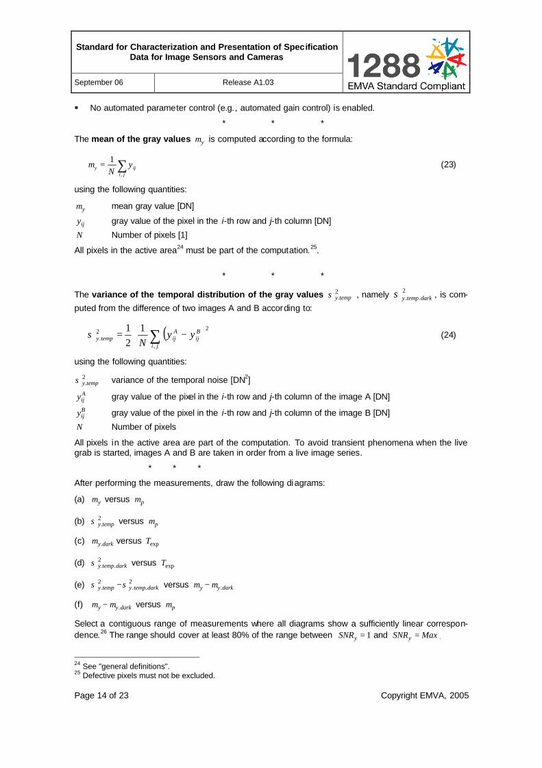
The mean of the gray values yµ is computed according to the formula:

∑=ji

ijy yN ,

1µ (23)

using the following quantities:

yµ mean gray value [DN]

ijy gray value of the pixel in the i-th row and j-th column [DN]

N Number of pixels [1]

All pixels in the active area24 must be part of the computation.25.

* * *

The variance of the temporal distribution of the gray values 2.tempyσ , namely 2

.. darktempyσ , is com-

puted from the difference of two images A and B according to:

( )

−= ∑

ji

Bij

Aijtempy yy

N ,

22.

121

σ (24)

using the following quantities:

2.tempyσ variance of the temporal noise [DN2]

Aijy gray value of the pixel in the i-th row and j-th column of the image A [DN] Bijy gray value of the pixel in the i-th row and j-th column of the image B [DN]

N Number of pixels

All pixels in the active area are part of the computation. To avoid transient phenomena when the live grab is started, images A and B are taken in order from a live image series.

* * *

After performing the measurements, draw the following diagrams:

(a) yµ versus pµ

(b) 2.tempyσ versus pµ

(c) darky.µ versus expT

(d) 2.. darktempyσ versus expT

(e) 2..

2. darktempytempy σσ − versus darkyy .µµ −

(f) darkyy .µµ − versus pµ

Select a contiguous range of measurements where all diagrams show a sufficiently linear correspon-dence.26 The range should cover at least 80% of the range between 1=ySNR and MaxSNRy = .

24 See "general definitions". 25 Defective pixels must not be excluded.




* * *

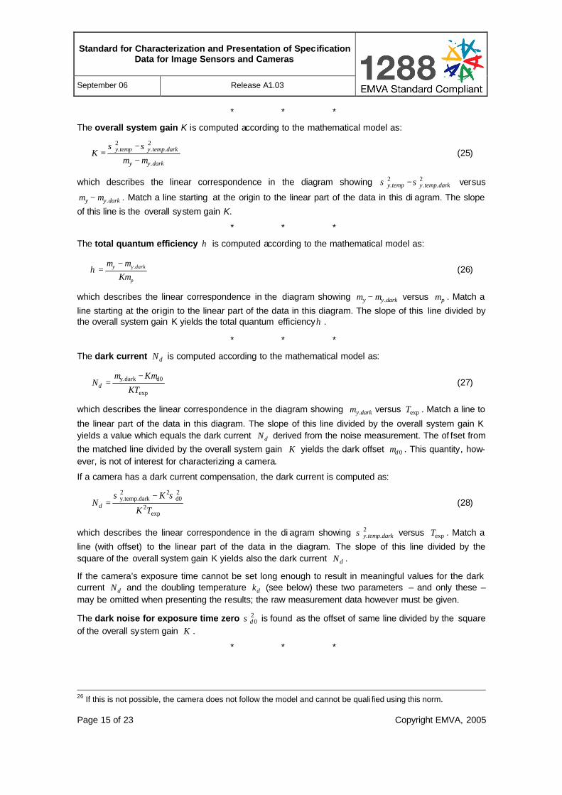
The overall system gain K is computed according to the mathematical model as:

darkyy

darktempytempyK.

2..

2.

µµ

σσ

−

−= (25)

which describes the linear correspondence in the diagram showing 2..

2. darktempytempy σσ − versus

darkyy .µµ − . Match a line starting at the origin to the linear part of the data in this di agram. The slope

of this line is the overall system gain K.

* * *

The total quantum efficiency η is computed according to the mathematical model as:

p

darkyy

Kµµµ

η .−= (26)

which describes the linear correspondence in the diagram showing darkyy .µµ − versus pµ . Match a

line starting at the origin to the linear part of the data in this diagram. The slope of this line divided by the overall system gain K yields the total quantum efficiencyη .

* * *

The dark current dN is computed according to the mathematical model as:

exp

d0y.dark

KT

KNd

µµ −= (27)

which describes the linear correspondence in the diagram showing darky.µ versus expT . Match a line to

the linear part of the data in this diagram. The slope of this line divided by the overall system gain K yields a value which equals the dark current dN derived from the noise measurement. The of fset from the matched line divided by the overall system gain K yields the dark offset 0dµ . This quantity, how-ever, is not of interest for characterizing a camera.

If a camera has a dark current compensation, the dark current is computed as:

exp2

2d0

22ky.temp.dar

TK

KNd

σσ −= (28)

which describes the linear correspondence in the di agram showing 2.. darktempyσ versus expT . Match a

line (with offset) to the linear part of the data in the diagram. The slope of this line divided by the square of the overall system gain K yields also the dark current dN .

If the camera’s exposure time cannot be set long enough to result in meaningful values for the dark current dN and the doubling temperature dk (see below) these two parameters – and only these –may be omitted when presenting the results; the raw measurement data however must be given.

The dark noise for exposure time zero 20dσ is found as the offset of same line divided by the square

of the overall system gain K .

* * *

26 If this is not possible, the camera does not follow the model and cannot be quali fied using this norm.




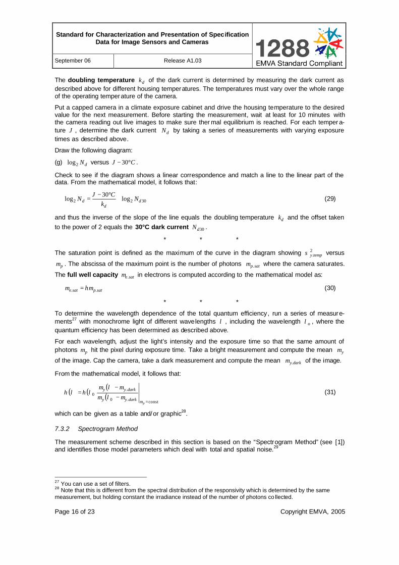
The doubling temperature dk of the dark current is determined by measuring the dark current as described above for different housing temperatures. The temperatures must vary over the whole range of the operating temperature of the camera.

Put a capped camera in a climate exposure cabinet and drive the housing temperature to the desired value for the next measurement. Before starting the measurement, wait at least for 10 minutes with the camera reading out live images to make sure ther mal equilibrium is reached. For each temper a-ture ϑ , determine the dark current dN by taking a series of measurements with varying exposure times as described above.

Draw the following diagram:

(g) dN2log versus C°− 30ϑ .

Check to see if the diagram shows a linear correspondence and match a line to the linear part of the data. From the mathematical model, it follows that:

3022 log30

log dd

d Nk

CN +

°−=

ϑ (29)

and thus the inverse of the slope of the line equals the doubling temperature dk and the offset taken to the power of 2 equals the 30°C dark current 30dN .

* * *

The saturation point is defined as the maximum of the curve in the diagram showing 2.tempyσ versus

pµ . The abscissa of the maximum point is the number of photons satp.µ where the camera saturates.

The full well capacity sate.µ in electrons is computed according to the mathematical model as:

satpsate .. ηµµ = (30)

* * *

To determine the wavelength dependence of the total quantum efficiency, run a series of measure-ments27 with monochrome light of different wavelengths λ , including the wavelength oλ , where the quantum efficiency has been determined as described above.

For each wavelength, adjust the light’s intensity and the exposure time so that the same amount of photons pµ hit the pixel during exposure time. Take a bright measurement and compute the mean yµ

of the image. Cap the camera, take a dark measurement and compute the mean darky.µ of the image.

From the mathematical model, it follows that:

( ) ( ) ( )( )

const.0

.0

=−

−=

pdarkyy

darkyy

µµλµ

µλµληλη (31)

which can be given as a table and/or graphic28.

7.3.2 Spectrogram Method

The measurement scheme described in this section is based on the “Spectrogram Method” (see [1]) and identifies those model parameters which deal with total and spatial noise.29

27 You can use a set of filters. 28 Note that this is different from the spectral distribution of the responsivity which is determined by the same measurement, but holding constant the irradiance instead of the number of photons co llected.




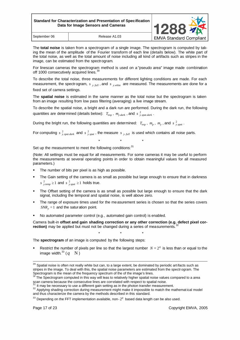
The total noise is taken from a spectrogram of a single image. The spectrogram is computed by tak-ing the mean of the amplitude of the Fourier transform of each line (details below). The white part of the total noise, as well as the total amount of noise including all kind of artifacts such as stripes in the image, can be estimated from the spectrogram.

For linescan cameras the spectrogram method is used on a "pseudo area" image made combination off 1000 consecutively acquired lines.30

To describe the total noise, three measurements for different lighting conditions are made. For each measurement, the spectrogram, fully.σ , and whitey.σ are measured. The measurements are done for a

fixed set of camera settings.

The spatial noise is estimated in the same manner as the total noise but the spectrogram is taken from an image resulting from low pass filtering (averaging) a live image stream.

To describe the spatial noise, a bright and a dark run are performed. During the dark run, the following quantities are determined (details below): expT , darky.µ , and 2

.. darkspatyσ .

During the bright run, the following quantities are determined: expT , pµ , yµ , and 2.spatyσ .

For computing 2.. darkspatyσ and 2

.spatyσ , the measure fully.σ is used which contains all noise parts.

* * *

Set up the measurement to meet the following conditions:31

(Note: All settings must be equal for all measurements. For some cameras it may be useful to perform the measurements at several operating points in order to obtain meaningful values for all measured parameters.)

§ The number of bits per pixel is as high as possible.

§ The Gain setting of the camera is as small as possible but large enough to ensure that in darkness 12

. ≥tempyσ and 12. ≥spatyσ holds true.

§ The Offset setting of the camera is as small as possible but large enough to ensure that the dark signal, including the temporal and spatial noise, is well above zero.

§ The range of exposure times used for the measurement series is chosen so that the series covers 1=ySNR and the saturation point.

§ No automated parameter control (e.g., automated gain control) is enabled.

Camera built-in offset and gain shading correction or any other correction (e.g. defect pixel cor-rection) may be applied but must not be changed during a series of measurements.32

* * *

The spectrogram of an image is computed by the following steps:

§ Restrict the number of pixels per line so that the largest number qN 2= is less than or equal to the image width.33 ( Ν∈q )

29 Spatial noise is often not really white but can, to a large extent, be dominated by periodic art ifacts such as stripes in the image. To deal with this, the spatial noise parameters are estimated from the spectr ogram. The Spectrogram is the mean of the frequency spectrum of the of the image’s lines. 30 The Spectrogram computed in this way will leas to relatively higher spatial noise values compared to a area scan camera because the consecutive lines are correlated with respect to spatial noise. 31 It may be necessary to use a different gain setting as in the photon transfer measurement. 32 Applying shading correction during measurement might make it impossible to match the mathemat ical model and thus characterize the camera by the methods described in this standard. 33 Depending on the FFT implementation available, non- q2 based data length can be also used.




§ For each of the M lines of the image, compute the amplitude of the Fourier transform:

− Prepare an array ( )ky with the length N2 .

− Copy the pixels from the image to the first half of the array ( 10 −≤≤ Nk ).

− Compute the mean of the pixels in the first half of the array

( )∑−

=

=1

0

1 N

k

kyN

y (32)

− Subtract the mean from the values

( ) ( ) ykyky −=: (33)

− Fill the second half of the array with zeros ( 12 −≤≤ NkN ).

− Apply a (Fast) Fourier Tr ansformation to the array y(k):

( ) ( )∑−

=

=12

0

22N

k

Nnk

jekynY

π (34)

The frequency index n runs in the interval Nn ≤≤0 yielding N+1 complex result values. Verify that the first value ( )0Y is zero. (This must be the case if the mean was subtracted from each line and computation was done correctly)

− Compute the amplitude of the Fourier transform as:

( ) ( ) ( )nYnYnY *= (35)

§ Take the squared mean of the amplitude values for all M lines of the image

( ) ( )∑=j

j nYM

nY21

(36)

where ( )nY j is the amplitude of the Fourier transform of the j-th line.

The N+1 values ( )nY with Nn ≤≤0 form the spectrogram of the image. It should be flat with occa-sional peaks only.

* * * The mean of the squared transform is the variance of the noise, describing the total grey value noise, including all artifacts. It is computed according to:

( )∑+=

nfully nY

N

22. 1

1σ (37)

The square of the height of the flat part seen in the spectrogram curve is the variance describing the

white part of the noise. It is estimated by taking the median of the spectrogram; sort the values ( )nY

and take the value with the index 2N .

( )( )2

. ,2,1,0sort Nindexwhitey NnnY

=== Kσ (38)

* * *

To check if the total noise is white, take three spectrograms: one in darkness, one with the camera at 50% saturation capacity sate.µ and one with the camera at 90% saturation. Draw the three spectro-




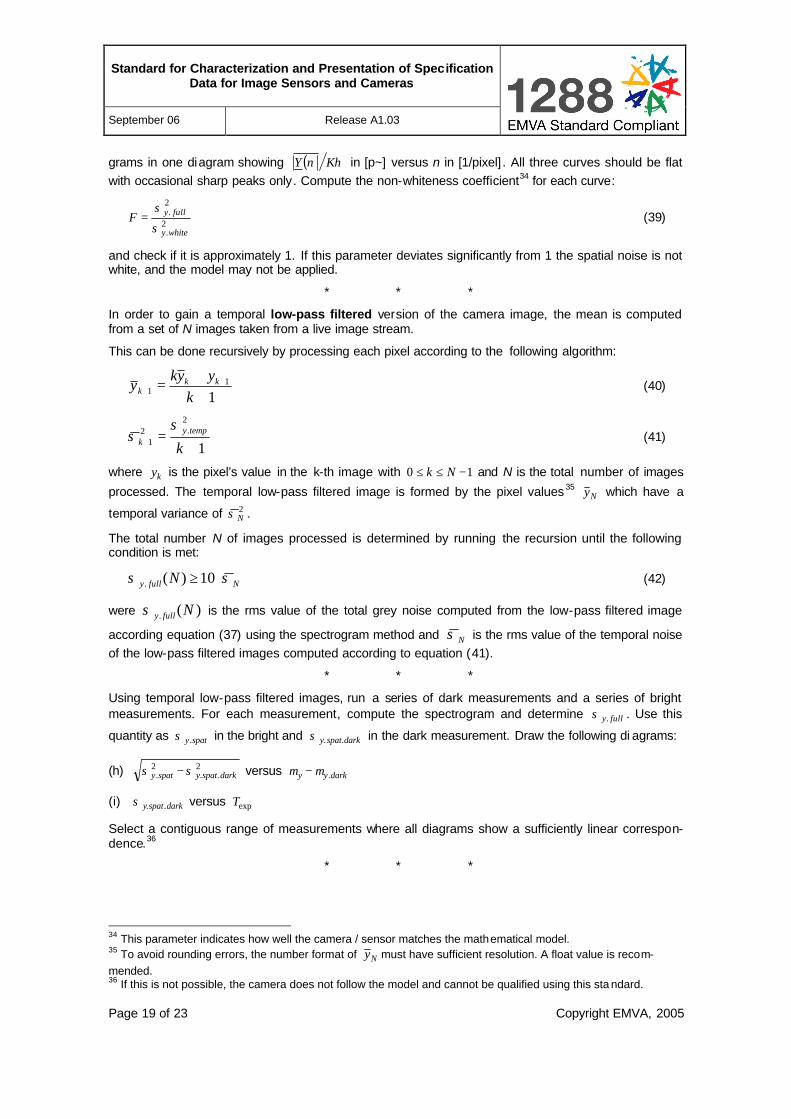
grams in one diagram showing ( ) ηKnY in [p~] versus n in [1/pixel] . All three curves should be flat with occasional sharp peaks only. Compute the non-whiteness coefficient34 for each curve:

2.

2.

whitey

fullyFσ

σ= (39)

and check if it is approximately 1. If this parameter deviates significantly from 1 the spatial noise is not white, and the model may not be applied.

* * *

In order to gain a temporal low-pass filtered version of the camera image, the mean is computed from a set of N images taken from a live image stream.

This can be done recursively by processing each pixel according to the following algorithm:

11

1 ++

= ++ k

yyky kk

k (40)

1

2.2

1 +=+ k

tempyk

σσ (41)

where ky is the pixel’s value in the k-th image with 10 −≤≤ Nk and N is the total number of images

processed. The temporal low-pass filtered image is formed by the pixel values 35 Ny which have a

temporal variance of 2Nσ .

The total number N of images processed is determined by running the recursion until the following condition is met:

Nfully N σσ ⋅≥10)(. (42)

were )(. Nfullyσ is the rms value of the total grey noise computed from the low-pass filtered image

according equation (37) using the spectrogram method and Nσ is the rms value of the temporal noise of the low-pass filtered images computed according to equation (41).

* * *

Using temporal low-pass filtered images, run a series of dark measurements and a series of bright measurements. For each measurement, compute the spectrogram and determine fully.σ . Use this

quantity as spaty.σ in the bright and darkspaty ..σ in the dark measurement. Draw the following di agrams:

(h) 2..

2. darkspatyspaty σσ − versus darkyy .µµ −

(i) darkspaty ..σ versus expT

Select a contiguous range of measurements where all diagrams show a sufficiently linear correspon-dence.36

* * *

34 This parameter indicates how well the camera / sensor matches the mathematical model. 35 To avoid rounding errors, the number format of Ny must have sufficient resolution. A float value is recom-mended. 36 If this is not possible, the camera does not follow the model and cannot be qualified using this sta ndard.




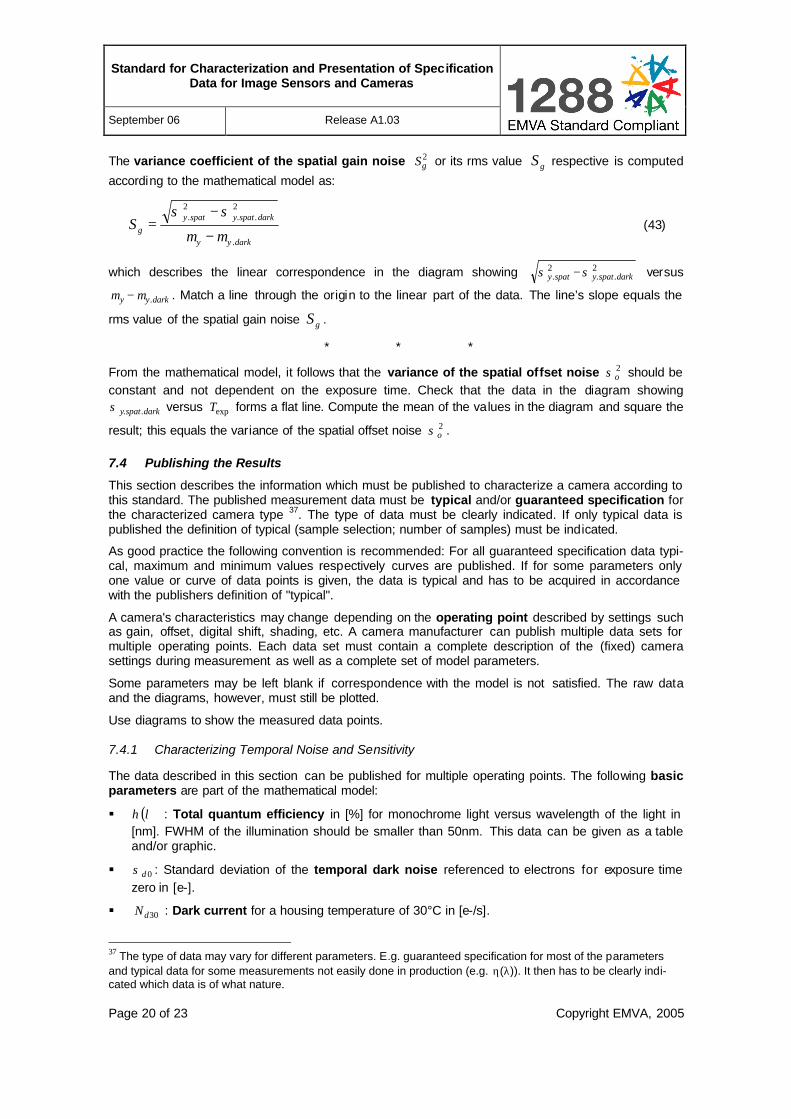
The variance coefficient of the spatial gain noise 2gS or its rms value gS respective is computed

according to the mathematical model as:

darkyy

darkspatyspatygS

.

2..

2.

µµ

σσ

−

−= (43)

which describes the linear correspondence in the diagram showing 2..

2. darkspatyspaty σσ − versus

darkyy .µµ − . Match a line through the origin to the linear part of the data. The line’s slope equals the

rms value of the spatial gain noise gS .

* * *

From the mathematical model, it follows that the variance of the spatial offset noise 2oσ should be

constant and not dependent on the exposure time. Check that the data in the diagram showing

darkspaty ..σ versus expT forms a flat line. Compute the mean of the values in the diagram and square the

result; this equals the variance of the spatial offset noise 2oσ .

7.4 Publishing the Results

This section describes the information which must be published to characterize a camera according to this standard. The published measurement data must be typical and/or guaranteed specification for the characterized camera type 37. The type of data must be clearly indicated. If only typical data is published the definition of typical (sample selection; number of samples) must be indicated.

As good practice the following convention is recommended: For all guaranteed specification data typi-cal, maximum and minimum values respectively curves are published. If for some parameters only one value or curve of data points is given, the data is typical and has to be acquired in accordance with the publishers definition of "typical".

A camera's characteristics may change depending on the operating point described by settings such as gain, offset, digital shift, shading, etc. A camera manufacturer can publish multiple data sets for multiple operating points. Each data set must contain a complete description of the (fixed) camera settings during measurement as well as a complete set of model parameters.

Some parameters may be left blank if correspondence with the model is not satisfied. The raw data and the diagrams, however, must still be plotted.

Use diagrams to show the measured data points.

7.4.1 Characterizing Temporal Noise and Sensitivity

The data described in this section can be published for multiple operating points. The following basic parameters are part of the mathematical model:

§ ( )λη : Total quantum efficiency in [%] for monochrome light versus wavelength of the light in [nm]. FWHM of the illumination should be smaller than 50nm. This data can be given as a table and/or graphic.

§ 0dσ : Standard deviation of the temporal dark noise referenced to electrons for exposure time zero in [e-].

§ 30dN : Dark current for a housing temperature of 30°C in [e-/s].

37 The type of data may vary for different parameters. E.g. guaranteed specification for most of the parameters and typical data for some measurements not easily done in production (e.g. η(λ)). It then has to be clearly indi-cated which data is of what nature.




§ dk : Doubling temperature of the dark current in [°C].

§ K1

: Inverse of overall system gain in [e-/DN].

§ sate.µ : Saturation capacity referenced to electrons in [e-].

The following derived data is computed from the mathematical model using the basic parameters given above:

§ ( )λµ min.p : Absolute sensitivity threshold in [p~] for monochrome light versus wavelength of the

light in [nm].

§ ( )pySNR µ : Signal to noise ratio in [1] versus number of photons collected in a pixel during expo-

sure time in [p~] for monochrome light with it’s wavelength given in [nm]. The wavelength should be near the maximum of the quantum efficiency. If this data is given as a diagram, it must be plot-ted with ySNR on the y-axis using a double scale 2log [bit] / 20 10log [dB] and pµ on the x-axis

using a single scale 2log [bit].

§ outin DYNDYN = : Dynamic range in [1]

The following raw measurement data is given in graphic form allowing the reader to estimate how well the camera follows the mathematical model. In all graphics, the linear part of the data used for estimating the parameters must be indicated.

§ ( )py µµ : Mean gray value in [DN] versus number of photons collected in a pixel during exp osure

time in [p~].

§ ( )ptempy µσ 2. : Variance of temporal distribution of gray values in [DN2] versus number of photons

collected in a pixel during exposure time in [p~].

§ ( )exp. Tdarkyµ : Mean of the gray values’ dark signal in [DN] versus exposure time in [s].

§ ( )exp2

.. Tdarktempyσ : Variance of the gray values’ temporal distribution in dark in [DN2] versus expo-

sure time in [s].

§ [ ]( )darkyydarktempytempy .2

..2

. µµσσ −− : Light induced variance of temporal distribution of gray values

in [DN2] versus light induced mean gray value in [DN].

§ [ ]( )pdarkyy µµµ .− : light induced mean gray value in [DN] versus the number of photons col-

lected in a pixel during exposure time in [p~].

§ ( )CNd °− 30log2 ϑ : logarithm to the base 2 of the dark current in [e-/s] versus devi ation of the housing temperature from 30°C in [°C]

7.4.2 Characterizing Total and Spatial Noise

The data described in this section can be published for multiple operating points. The following basic parameters are part of the mathematical model:

§ oσ : Standard deviation of the spatial offset noise referenced to electrons in [e-].

§ gS : Standard deviation of the spatial gain noise in [%].




§ ( )ηK

nY : Spectrogram referenced to photons in [p~] versus spatial frequency in [1/pixel] for no

light, 50% saturation and 90% saturation. Indicate the whiteness factor F for each of the three graphs.

The following raw measurement data is given in graphic form allowing the reader to estimate how well the camera follows the mathematical model. In all graphics, the linear part of the data used for estimating the parameters must be indicated.

§ ( )darkyydarkspatyspaty .2

..2

. µµσσ −− : Light induced standard deviation of the spatial noise in [DN] ver-

sus light induced mean of gray values [DN].

§ ( )exp.. Tdarkspatyσ : Standard deviation of the spatial dark noise in [DN] versus exposure time in [s].




8 References [1] Dierks, Friedrich, “Sensitivity and Image Quality of Digital Cameras”, download at

http://www.baslerweb.com/ [2] Holst, Gerald, “CCD arrays, cameras, and displays”, JCD Publishing, 1998, ISBN 0-9640000-4-0 [3] Jähne, Bernd, Practical Handbook on Image Processing for Scientific and Technical Applications,

CRC Press 2004, ISBN [4] Janesick, James R., CCD characterization using the photon transfer technique, Proc. SPIE Vol.

570, Solid State Imaging Arrays, K. Pretty johns and E. Derenlak, Eds., pp. 7-19 (1985) [5] Janesick, James R., Scientific Charge-Coupled Devices, SPIE PRESS Monograph Vol. PM83,

ISBN 0-8194-3698-4 [6] Kammeyer, Karl, Kroschel, Kristian, Digitale Signalverarbeitung, Teubner Stuttgart 1989, ISBN 3-

519-06122-8 [7] Theuwissen, Albert J.P., Solid-State Imaging with Charge-Coupled Devices, Kluwer Academic

Publishers 1995, ISBN 0-7923-3456-6

emva standard 1288 · jai/pulnix tue moerk ... all pixels start exposing and stop exposing at the...

Documents