emva standard 1288 - zenodo.org

EMVA Standard 1288

Standard for Characterization of ImageSensors and Cameras

Release 3.0

November 29, 2010

Issued by

European Machine Vision Association

www.emva.org

Contents

1 Introduction and Scope . . . . . . . . . . . . . . . . . . . . . . . . . . . . . . . . 42 Sensitivity, Linearity, and Noise . . . . . . . . . . . . . . . . . . . . . . . . . . . 5

2.1 Linear Signal Model . . . . . . . . . . . . . . . . . . . . . . . . . . . . . . . 52.2 Noise Model . . . . . . . . . . . . . . . . . . . . . . . . . . . . . . . . . . . 62.3 Signal-to-Noise Ratio (SNR) . . . . . . . . . . . . . . . . . . . . . . . . . . 72.4 Signal Saturation and Absolute Sensitivity Threshold . . . . . . . . . . . . 7

3 Dark Current . . . . . . . . . . . . . . . . . . . . . . . . . . . . . . . . . . . . . 83.1 Mean and Variance . . . . . . . . . . . . . . . . . . . . . . . . . . . . . . . 83.2 Temperature Dependence . . . . . . . . . . . . . . . . . . . . . . . . . . . . 8

4 Spatial Nonuniformity and Defect Pixels . . . . . . . . . . . . . . . . . . . . . . 84.1 Spatial Variances, DSNU, and PRNU . . . . . . . . . . . . . . . . . . . . . 94.2 Types of Nonuniformities . . . . . . . . . . . . . . . . . . . . . . . . . . . . 94.3 Defect Pixels . . . . . . . . . . . . . . . . . . . . . . . . . . . . . . . . . . . 10

4.3.1 Logarithmic Histograms. . . . . . . . . . . . . . . . . . . . . . . . . . 104.3.2 Accumulated Histograms. . . . . . . . . . . . . . . . . . . . . . . . . 11

4.4 Highpass Filtering . . . . . . . . . . . . . . . . . . . . . . . . . . . . . . . . 115 Overview Measurement Setup and Methods . . . . . . . . . . . . . . . . . . . . 126 Methods for Sensitivity, Linearity, and Noise . . . . . . . . . . . . . . . . . . . . 12

6.1 Geometry of Homogeneous Light Source . . . . . . . . . . . . . . . . . . . . 126.2 Spectral Properties of Light Source . . . . . . . . . . . . . . . . . . . . . . . 136.3 Variation of Irradiation . . . . . . . . . . . . . . . . . . . . . . . . . . . . . 146.4 Calibration of Irradiation . . . . . . . . . . . . . . . . . . . . . . . . . . . . 146.5 Measurement Conditions for Linearity and Sensitivity . . . . . . . . . . . . 156.6 Evaluation of the Measurements according to the Photon Transfer Method 15

www.emva.org

bjaehne

Schreibmaschinentext

doi: 10.5281/zenodo.10696

Standard for Characterizationof Image Sensors and CamerasRelease 3.0, Nov. 29, 2010

6.7 Evaluation of Linearity . . . . . . . . . . . . . . . . . . . . . . . . . . . . . 197 Methods for Dark Current . . . . . . . . . . . . . . . . . . . . . . . . . . . . . . 19

7.1 Evaluation of Dark Current at One Temperature . . . . . . . . . . . . . . . 197.2 Evaluation of Dark Current with Temperatures . . . . . . . . . . . . . . . . 19

8 Methods for Spatial Nonuniformity and Defect Pixels . . . . . . . . . . . . . . . 218.1 Spatial Standard Deviation, DSNU, PRNU . . . . . . . . . . . . . . . . . . 218.2 Horizontal and Vertical Spectrograms . . . . . . . . . . . . . . . . . . . . . 248.3 Defect Pixel Characterization . . . . . . . . . . . . . . . . . . . . . . . . . . 25

9 Methods for Spectral Sensitivity . . . . . . . . . . . . . . . . . . . . . . . . . . . 289.1 Spectral Light Source Setup . . . . . . . . . . . . . . . . . . . . . . . . . . . 289.2 Measuring Conditions . . . . . . . . . . . . . . . . . . . . . . . . . . . . . . 289.3 Calibration . . . . . . . . . . . . . . . . . . . . . . . . . . . . . . . . . . . . 289.4 Evaluation . . . . . . . . . . . . . . . . . . . . . . . . . . . . . . . . . . . . 28

10 Publishing the Results . . . . . . . . . . . . . . . . . . . . . . . . . . . . . . . . 2910.1 Basic Information . . . . . . . . . . . . . . . . . . . . . . . . . . . . . . . . 3010.2 The EMVA 1288 Parameters . . . . . . . . . . . . . . . . . . . . . . . . . . 3010.3 The EMVA 1288 Datasheet . . . . . . . . . . . . . . . . . . . . . . . . . . . 3010.4 Template Datasheet . . . . . . . . . . . . . . . . . . . . . . . . . . . . . . . 31

A Bibliography . . . . . . . . . . . . . . . . . . . . . . . . . . . . . . . . . . . . . . 31B Notation . . . . . . . . . . . . . . . . . . . . . . . . . . . . . . . . . . . . . . . . 32C Changes to Release A2.01 . . . . . . . . . . . . . . . . . . . . . . . . . . . . . . 33

C.1 Added Features . . . . . . . . . . . . . . . . . . . . . . . . . . . . . . . . . . 33C.2 Extension of Methods to Vary Irradiation . . . . . . . . . . . . . . . . . . . 33C.3 Modifications in Conditions and Procedures . . . . . . . . . . . . . . . . . . 33C.4 Limit for Minimal Temporal Standard Deviation; Introduction of Quantiza-

tion Noise . . . . . . . . . . . . . . . . . . . . . . . . . . . . . . . . . . . . . 34C.5 Highpass Filtering with Nonuniformity Measurements . . . . . . . . . . . . 35

2 of 36 c© Copyright EMVA, 2010


Acknowledgements

Please refer to www.standard1288.org for the list of contributors to the Standard.EMVA 1288 is an initiative driven by the industry and living from the personal initiative

of the supporting companies and institutions delegates as well as from the support of theseorganizations. Thanks to this generosity the presented document can be provided free ofcharge to the users of this standard. EMVA thanks those contributors in the name of thewhole vision community.

Rights and Trademarks

The European Machine Vision Association owns the ”EMVA, standard 1288 compliant” logo.Any company can obtain a license to use the ”EMVA standard 1288 compliant” logo, freeof charge, with product specifications measured and presented according to the definitionsin EMVA standard 1288. The licensee guarantees that he meets the terms of use in therelevant release of EMVA standard 1288. Licensed users will self-certify compliance of theirmeasurement setup, computation and representation with which the ”EMVA standard 1288compliant” logo is used. The licensee has to check regularly compliance with the relevantrelease of EMVA standard 1288, at least once a year. When displayed on line the logo hasto be featured with a link to EMVA standardization web page. EMVA will not be liablefor specifications not compliant with the standard and damage resulting there from. EMVAkeeps the right to withdraw the granted license any time and without giving reasons.

About this Standard

EMVA has started the initiative to define a unified method to measure, compute and presentspecification parameters and characterization data for cameras and image sensors used formachine vision applications. The standard does not define what nature of data should bedisclosed. It is up to the component manufacturer to decide if he wishes to publish typicaldata, data of an individual component, guaranteed data, or even guaranteed performanceover life time of the component. However the component manufacturer shall clearly indicatewhat the nature of the presented data is. The standard is organized in different sections,each addressing a group of specification parameters, assuming a certain physical behaviorof the sensor or camera under certain boundary conditions. Additional sections coveringmore parameters and a wider range of sensor and camera products will be added succes-sively. There are compulsory sections, of which all measurements must be made and ofwhich all required data and graphics must be included in a datasheet using the EMVA1288logo. Further there are optional sections which may be skipped for a component where therespective data is not relevant or the mathematical model is not applicable. Each datasheetshall clearly indicate which sections of the EMVA1288 standard are enclosed.

It may be necessary for the manufacturer to indicate additional, component specificinformation, not defined in the standard, to fully describe the performance of image sensoror camera products, or to describe physical behavior not covered by the mathematical modelsof the standard. It is possible in accordance with the EMVA1288 standard to include suchdata in the same datasheet. However the data obtained by procedures not described in thecurrent release of the EMVA1288 standard must be clearly designated and grouped in aseparate section. It is not permitted to use parameter designations defined in any of theEMVA1288 modules for such additional information not acquired or presented accordingthe EMVA1288 procedures.

The standard is intended to provide a concise definition and clear description of themeasurement process and to benefit the Automated Vision Industry by providing fast, com-prehensive and consistent access to specification information for cameras and sensors. It willbe particularly beneficial for those who wish to compare cameras or who wish to calculatesystem performance based on the performance specifications of an image sensor or a camera.

c© Copyright EMVA, 2010 3 of 36

www.standard1288.org


1 Introduction and Scope

This release of the standard covers monochrome and color digital cameras with linear photoresponse characteristics. It is valid for area scan and line scan cameras. Analog camerascan be described according to this standard in conjunction with a frame grabber; similarly,image sensors can be described as part of a camera. If not specified otherwise, the termcamera is used for all these items.

The standard text is parted into four sections describing the mathematical model andparameters that characterize cameras and sensors with respect to

• Section 2: linearity, sensitivity, and noise for monochrome and color cameras,

• Section 3: dark current,

• Section 4: sensor array nonuniformities and defect pixels characterization,

a section with an overview of the required measuring setup (Section 5), and five sectionsthat detail the requirements for the measuring setup and the evaluation methods for

• Section 6: linearity, sensitivity, and noise,

• Section 7: dark current,

• Section 8: sensor array nonuniformities and defect pixels characterization,

• Section 9: spectral sensitivity,

The detailed setup is not regulated in order not to hinder progress and the ingenuity ofthe implementers. It is, however, mandatory that the measuring setups meet the propertiesspecified by the standard. Section 10 finally describes how to produce the EMVA 1288datasheets. Appendix B describes the notation and Appendix C details the changes torelease 2

It is important to note that the standard can only be applied if the camera under test canactually be described by the mathematical model on which the standard is based. If theseconditions are not fulfilled, the computed parameters are meaningless with respect to thecamera under test and thus the standard cannot be applied. Currently, electron multiplyingcameras (EM CCD, [1, 2]) and cameras that are sensitive in the deep ultraviolet, where morethan one electron per absorbed photon is generated [5], are not covered by the standard.The general assumptions include

1. The amount of photons collected by a pixel depends on the product of irradiance E(units W/m2) and exposure time texp (units s), i. e., the radiative energy density Etexp

at the sensor plane.

2. The sensor is linear, i. e., the digital signal y increases linear with the number of photonsreceived.

3. All noise sources are wide-sense stationary and white with respect to time and space.The parameters describing the noise are invariant with respect to time and space.

4. Only the total quantum efficiency is wavelength dependent. The effects caused by lightof different wavelengths can be linearly superimposed.

5. Only the dark current is temperature dependent.

These assumptions describe the properties of an ideal camera or sensor. A real sensor willdepart more or less from an ideal sensor. As long as the deviation is small, the description isstill valid and it is one of the tasks of the standard to describe the degree of deviation froman ideal behavior. However, if the deviation is too large, the parameters derived may be toouncertain or may even render meaningless. Then the camera cannot be characterized usingthis standard. The standard can also not be used for cameras that clearly deviate from oneof these assumptions. For example, a camera with a logarithmic instead of a linear responsecurve cannot be described with the present release of the standard.



a

42

A number of photons ...

... hitting the pixel area during exposure time ...

... creating a number of electrons ...

... forming a charge which is converted by a capacitor to a voltage ...

... being amplified ...

... and digitized ...

... resulting in the digital gray value.

b

pe

K yηnn

dnquantumefficiency

system gain

number ofphotons

number ofelectrons

digital grey value

dark noise quantization noise

qσ

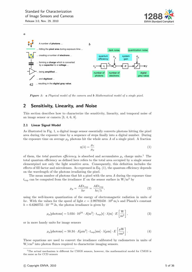
Figure 1: a Physical model of the camera and b Mathematical model of a single pixel.

2 Sensitivity, Linearity, and Noise

This section describes how to characterize the sensitivity, linearity, and temporal noise ofan image sensor or camera [3, 4, 6, 8].

2.1 Linear Signal Model

As illustrated in Fig. 1, a digital image sensor essentially converts photons hitting the pixelarea during the exposure time by a sequence of steps finally into a digital number. Duringthe exposure time on average µp photons hit the whole area A of a single pixel. A fraction

η(λ) =µeµp

(1)

of them, the total quantum efficiency, is absorbed and accumulates µe charge units.1 Thetotal quantum efficiency as defined here refers to the total area occupied by a single sensorelementpixel not only the light sensitive area. Consequently, this definition includes theeffects of fill factor and microlenses. As expressed in Eq. (1), the quantum efficiency dependson the wavelength of the photons irradiating the pixel.

The mean number of photons that hit a pixel with the area A during the exposure timetexp can be computed from the irradiance E on the sensor surface in W/m2 by

µp =AEtexp

hν=AEtexp

hc/λ, (2)

using the well-known quantization of the energy of electromagnetic radiation in units ofhν. With the values for the speed of light c = 2.99792458 · 108 m/s and Planck’s constanth = 6.6260755 · 10−34 Js, the photon irradiance is given by

µp[photons] = 5.034 · 1024 ·A[m2] · texp[s] · λ[m] · E[

W

m2

], (3)

or in more handy units for image sensors

µp[photons] = 50.34 ·A[µm2] · texp[ms] · λ[µm] · E[µW

cm2

]. (4)

These equations are used to convert the irradiance calibrated by radiometers in units ofW/cm2 into photon fluxes required to characterize imaging sensors.

1The actual mechanism is different for CMOS sensors, however, the mathematical model for CMOS isthe same as for CCD sensors



In the camera electronics, the charge units accumulated by the photo irradiance isconverted into a voltage, amplified, and finally converted into a digital signal y by an analogdigital converter (ADC). The whole process is assumed to be linear and can be described bya single quantity, the overall system gain K with units DN/e−, i. e., digits per electrons.2

Then the mean digital signal µy results in

µy = K(µe + µd) or µy = µy.dark +Kµe, (5)

where µd is the mean number electrons present without light, which result in the meandark signal µy.dark = Kµd in units DN with zero irradiation. Note that the dark signalwill generally depend on other parameters, especially the exposure time and the ambienttemperature (Section 3).

With Eqs. (1) and (2), Eq. (5) results in a linear relation between the mean gray valueµy and the number of photons irradiated during the exposure time onto the pixel:

µy = µy.dark +Kη µp = µy.dark +KηλA

hcE texp. (6)

This equation can be used to verify the linearity of the sensor by measuring the mean grayvalue in relation to the mean number of photons incident on the pixel and to measure theresponsivity Kη from the slope of the relation. Once the overall system gain K is determinedfrom Eq. (9), it is also possible to estimate the quantum efficiency from the responsivityKη.

2.2 Noise Model

The number of charge units (electrons) fluctuates statistically. According to the laws ofquantum mechanics, the probability is Poisson distributed. Therefore the variance of thefluctuations is equal to the mean number of accumulated electrons:

σ2e = µe. (7)

This noise, often referred to as shot noise is given by the basic laws of physics and equal forall types of cameras.

All other noise sources depend on the specific construction of the sensor and the cameraelectronics. Due to the linear signal model (Section 2.1), all noise sources add up. Forthe purpose of a camera model treating the whole camera electronics as a black box it issufficient to consider only two additional noise sources. All noise sources related to thesensor read out and amplifier circuits can be described by a signal independent normal-distributed noise source with the variance σ2

d. The final analog digital conversion (Fig. 1b)adds another noise source that is uniform-distributed between the quantization intervals andhas a variance σ2

q = 1/12 DN2 [8].Because the variance of all noise sources add up linear,the total temporal variance of the digital signal y, σ2

y, is given according to the laws of errorpropagation by

σ2y = K2

(σ2d + σ2

e

)+ σ2

q (8)

Using Eqs. (7) and (5), the noise can be related to the measured mean digital signal:

σ2y = K2σ2

d + σ2q︸︷︷︸

offset

+ K︸︷︷︸slope

(µy − µy.dark). (9)

This equation is central to the characterization of the sensor. From the linear relationbetween the variance of the noise σ2

y and the mean photo-induced gray value µy−µy.dark it ispossible to determine the overall system gain K from the slope and the dark noise varianceσ2d from the offset. This method is known as the photon transfer method [6, 7].

2DN is a dimensionless unit, but for sake of clarity, it is better to denote it specifically.



2.3 Signal-to-Noise Ratio (SNR)

The quality of the signal is expressed by the signal-to-noise ratio (SNR), which is defined as

SNR =µy − µy.dark

σy. (10)

Using Eqs. (6) and (8), the SNR can then be written as

SNR(µp) =ηµp√

σ2d + σ2

q/K2 + ηµp

. (11)

Except for the small effect caused by the quantification noise, the overall system gain Kcancels out so that the SNR depends only on the quantum efficiency η(λ) and the darksignal noise σd in units e−. Two limiting cases are of interest: the high-photon range withηµp � σ2

d + σ2q/K

2 and the low-photon range with ηµp � σ2d + σ2

q/K2:

SNR(µp) ≈

√ηµp, ηµp � σ2

d + σ2q/K

2,

ηµp√σ2d + σ2

q/K2, ηµp � σ2

d + σ2q/K

2.(12)

This means that the slope of the SNR curve changes from a linear increase at low irradiationto a slower square root increase at high irradiation.

A real sensor can always be compared to an ideal sensor with a quantum efficiencyη = 1, no dark noise (σd = 0) and negligible quantization noise (σq/K = 0). The SNR ofan ideal sensor is given by

SNRideal =√µp. (13)

Using this curve in SNR graphs, it becomes immediately visible how close a real sensorcomes to an ideal sensor.

2.4 Signal Saturation and Absolute Sensitivity Threshold

For an k-bit digital camera, the digital gray values are in a range between the 0 and 2k − 1.The practically useable gray value range is smaller, however. The mean dark gray valueµy.dark must be higher than zero so that no significant underflow occurs by temporal noiseand the dark signal nonuniformity (for an exact definition see Section 6.5). Likewise themaximal usable gray value is lower than 2k− 1 because of the temporal noise and the photoresponse nonuniformity.

Therefore, the saturation irradiation µp.sat is defined as the maximum of the measuredrelation between the variance of the gray value and the irradiation in units photons/pixel.The rational behind this definition is that according to Eq. (9) the variance is increasing withthe gray value but is decreasing again, when the digital values are clipped to the maximumdigital gray value 2k − 1.

From the saturation irradiation µp.sat the saturation capacity µe.sat can be computed:

µe.sat = ηµp.sat. (14)

The saturation capacity must not be confused with the full-well capacity. It is normallylower than the full-well capacity, because the signal is clipped to the maximum digital value2k − 1 before the physical saturation of the pixel is reached.

The minimum detectable irradiation or absolute sensitivity threshold, µp.min can be de-fined by using the SNR. It is the mean number of photons required so that the SNR is equalto one.

For this purpose, it is required to know the inverse function to Eq. (11), i. e., the numberof photons required to reach a given SNR. Inverting Eq. (11) results in

µp(SNR) =SNR2

2η

1 +

√1 +

4(σ2d + σ2

q/K2)

SNR2

. (15)



In the limit of large and small SNR, this equation approximates to

µp(SNR) ≈

SNR2

η

(1 +

σ2d + σ2

q/K2

SNR2

), SNR2 � σ2

d + σ2q/K

2,

SNR

η

(√σ2d + σ2

q/K2 +

SNR

2

), SNR2 � σ2

d + σ2q/K

2.

(16)

This means that for almost all cameras, i. e., when σ2d +σ2

q/K2 � 1, the absolute sensitivity

threshold can be well approximates by

µp(SNR = 1) = µp.min ≈1

η

(√σ2d + σ2

q/K2 +

1

2

)=

1

η

(σy.dark

K+

1

2

). (17)

The ratio of the signal saturation to the absolute sensitivity threshold is defined as thedynamic range (DR):

DR =µp.sat

µp.min. (18)

3 Dark Current

3.1 Mean and Variance

The dark signal µd introduced in the previous section, see Eq. (5), is not constant. Themain reason for the dark signal are thermally induced electrons. Therefore, the dark signalshould increase linearly with the exposure time

µd = µd.0 + µtherm = µd.0 + µItexp. (19)

In this equation all quantities are expressed in units of electrons (e−/pixel). These valuescan be obtained by dividing the measured values in the units DN by the overall system gainK (Eq. (9)).

The quantity µI is named the dark current, given in the units e−/(pixel s). Accordingto the laws of error propagation, the variance of the dark signal is then given as

σ2d = σ2

d.0 + σ2therm = σ2

d.0 + µItexp, (20)

because the thermally induced electrons are Poisson distributed as the light induced onesin Eq. (7) with σ2

therm = µtherm. If a camera or sensor has a dark current compensation thedark current can only be characterized using Eq. (20).

3.2 Temperature Dependence

The temperature dependence of the dark current is modeled in a simplified form. Becauseof the thermal generation of charge units, the dark current increases roughly exponentiallywith the temperature [4, 5, 11]. This can be expressed by

µI = µI.ref · 2(T−Tref)/Td . (21)

The constant Td has units K or ◦C and indicates the temperature interval that causes adoubling of the dark current. The temperature Tref is a reference temperature at which allother EMVA 1288 measurements are performed and µI.ref the dark current at the referencetemperature. The measurement of the temperature dependency of the dark current is theonly measurement to be performed at different ambient temperatures, because it is the onlycamera parameter with a strong temperature dependence.

4 Spatial Nonuniformity and Defect Pixels

The model discussed so far considered only a single pixel. All parameters of an array ofpixels, will however vary from pixel to pixel. Sometimes these nonuniformities are called



fixed pattern noise, or FPN. This expression is however misleading, because inhomogeneitiesare no noise, which makes the signal varying in time. The inhomogeneity may only bedistributed randomly. Therefore it is better to name this effect nonuniformity.

Essentially there are two basic nonuniformities. First, the dark signal can vary from pixelto pixel. This effect is called dark signal nonuniformity, abbreviated by DSNU. Second, thevariation of the sensitivity is called photo response nonuniformity, abbreviated by PRNU.

The EMVA 1288 standard describes nonuniformities in three different ways. The spatialvariance (Section 4.1) is a simply overall measure of the spatial nonuniformity. The spectro-gram method (Section 4.2) offers a way to analyze patterns or periodic spatial variations,which may be disturbing to image processing operations or the human observer. Finally,the characterization of defect pixels (Section 4.3) is a flexible method to specify unusable ordefect pixels according to application specific criteria.

4.1 Spatial Variances, DSNU, and PRNU

For all types of spatial nonuniformities, spatial variances can be defined. This results inequations that are equivalent to the temporal noise but with another meaning. The averagingis performed over all pixels of a sensor array. The mean of the M ×N dark and the 50%saturation images, ydark and y50, are given by:

µy.dark =1

MN

M−1∑m=0

N−1∑n=0

ydark[m][n], µy.50 =1

MN

M−1∑m=0

N−1∑n=0

y50[m][n], (22)

where M and N are the number of rows and columns of the image and m and n the rowand column indices of the array, respectively. Likewise, the spatial variances s2 of dark and50% saturation images are given by:

s2y.dark =

1

MN − 1

M−1∑m=0

N−1∑n=0

(ydark[m][n]− µy.dark)2, (23)

s2y.50 =

1

MN − 1

M−1∑m=0

N−1∑n=0

(y50[m][n]− µy.50)2. (24)

All spatial variances are denoted with the symbol s2 to distinguish them easily from thetemporal variances σ2.

The DSNU and PRNU values of the EMVA 1288 standard are based on spatial standarddeviations:

DSNU1288 = sy.dark/K (units e−),

PRNU1288 =

√s2y.50 − s2

y.dark

µy.50 − µy.dark· 100%.

(25)

The index 1288 has been added to these definitions because many different definitions ofthese quantities can be found in the literature. The DSNU1288 is expressed in units e−; bymultiplying with the overall system gain K it can also be given in units DN. The PRNU1288

is defined as a standard deviation relative to the mean value. In this way, the PRNU1288

gives the spatial standard deviation of the photoresponse nonuniformity in % from the mean.

4.2 Types of Nonuniformities

The variances defined in the previous sections give only an over-all measure of the spatialnonuniformity. It can, however, not be assumed in general that the spatial variations arenormally distributed. This would only be the case if the spatial variations are totally ran-dom, i. e., that there are no spatial correlation of the variations. However, for an adequatedescription of the spatial nonuniformities several effects must be considered:

Gradual variations. Manufacturing imperfections can cause gradual low-frequency vari-ations over the whole chip. This effect is not easy to measure because it requires a veryhomogeneous irradiation of the chip, which is difficult to achieve. Fortunately this effect



a b

OutlierLog

His

togr

am

x-Valueµx

Single Image Histogram

Averaged Image Histogram

σspat

σtotal

Figure 2: Logarithmic histogram of spatial variations a Showing comparison of data to model andidentification of deviations from the model and of outliers, b Comparison of logarithmic histogramsfrom single images and averaged over many images.

does not really degrade the image quality significantly. A human observer does not detectit at all and additional gradual variations are introduced by lenses (shading, vignetting)and nonuniform illumination. Therefore, gradual variations must be corrected with thecomplete image system anyway for applications that demand a flat response over thewhole sensor array.

Periodic variations. This type of distortion is caused by electronic interferences in thecamera electronic and is very nasty, because the human eye detects such distortionsvery sensitively. Likewise many image processing operations are disturbed. Thereforeit is important to detect this type of spatial variation. This can most easily be doneby computing a spectrogram, i. e., a power spectrum of the spatial variations. In thespectrogram, periodic variations show up as sharp peaks with specific spatial frequenciesin units cycles/pixel.

Outliers. This are single pixels or cluster of pixels that show a significantly deviation fromthe mean. This type of nonuniformity is discussed in detail in Section 4.3.

Random variations. If the spatial nonuniformity is purely random, i. e., shows no spatialcorrelation, the power spectrum is flat, i. e., the variations are distributed equally overall wavelengths. Such a spectrum is called a white spectrum.

From this description it is obvious that the computation of the spectrogram, i. e., thepower spectrum, is a good tool.

4.3 Defect Pixels

As application requirements differ, it will not be possible to find a common denominator toexactly define when a pixel is defective and when it is not. Therefore it is more appropriate toprovide statistical information about pixel properties in the form of histograms. In this wayan applicant can specify how many pixels are unusable or defect using application-specificcriteria.

4.3.1 Logarithmic Histograms. It is useful to plot the histograms with logarithmic y-axis for two reasons (Fig. 2a). Firstly, it is easy to compare the measured histograms with anormal distribution, which shows up as a negatively shaped parabola in a logarithmic plot.Thus it is easy to see deviations from normal distributions. Secondly, also rare outliers, i. e.,a few pixels out of millions of pixels can be seen easily.

All histograms have to be computed from pixel values that come from averaging overmany images. In this way the histograms only reflect the statistics of the spatial noise andthe temporal noise is averaged out. The statistics from a single image is different. It containsthe total noise, i.e. the spatial and the temporal noise. It is, however, useful to see in howfar the outliers of the averaged image histogram will vanish in the temporal noise (Fig. 2b).

It is hard to generally predict in how far a deviation from the model will impact thefinal applications. Some of them will have human spectators, while others use a variety of



Log

accu

mul

aged

H

isto

gram

(%)

Absolute Deviation from Mean Value µx

Dev

iatio

n

Outlier

Mod

el Stop

Ban

d

100

Figure 3: Accumulated histogram with logarithmic y-axis.

algorithms to make use of the images. While a human spectator is usually able to workwell with pictures in which some pixel show odd behaviors, some algorithms may sufferfrom it. Some applications will require defect-free images, some will tolerate some outliers,while other still have problems with a large number of pixels slightly deviating. All thisinformation can be read out of the logarithmic histograms.

4.3.2 Accumulated Histograms. A second type of histograms, accumulated histogramis useful in addition (Fig. 3). It is computed to determine the ratio of pixels deviating bymore than a certain amount. This can easily be connected to the application requirements.Quality criteria from camera or chip manufacturers can easily be drawn in this graph.Usually the criteria is, that only a certain amount of pixels deviates more than a certainthreshold. This can be reflected by a rectangular area in the graph. Here it is called stopband in analogy to drawings from high-frequency technologies that should be very familiarto electronics engineers.

4.4 Highpass Filtering

This section addresses the problem that the photoresponse distribution may be dominatedby gradual variations in illumination source, especially the typical fall-off of the irradiancetowards the edges of the sensor. Low-frequency spatial variations of the image sensor,however, are of less importance, because of two reasons. Firstly, lenses introduce a fall-offtowards the edges of an image (lens shading). Except for special low-shading lenses, thiseffect makes a significant contribution to the low-frequency spatial variations. Secondly,almost all image processing operations are not sensitive to gradual irradiation changes. (Seealso discussion in Section 4.2 under item gradual variations.)

In order to show the properties of the camera rather than the properties of an imperfectillumination system, a highpass filtering is applied before computing the histograms fordefect pixel characterization discussed in Sections 4.3.1–4.3.2. In this way the effect of lowspatial frequency sensor properties is suppressed. The highpass filtering is performed usinga box filter, for details see Appendix C.5.


Standard for Characterization

of Image Sensors and Cameras

Release 3.0, Nov. 29, 2010

Table 1: List of all EMVA 1288 measurements with classification into mandatory and optionalmeasurements.

Type of measurement Mandatory Reference

Sensitivity, temporal noise and linearity Y Section 6

Nonuniformity Y Sections 8.1 and 8.2

Defect pixel characterization Y Section 8.3

Dark current Y Section 7.1

Temperature dependence on dark current N Section 7.2

Spectral measurements η(λ) N Section 9

5 Overview Measurement Setup and Methods

The characterization according to the EMVA 1288 standard requires three different measur-ing setups:

1. A setup for the measurement of sensitivity, linearity and nonuniformity using a homoge-neous monochromatic light source (Sections 6 and 8).

2. The measurement of the temperature dependency of the dark current requires somemeans to control the temperature of the camera. The measurement of the dark currentat the standard temperature requires no special setup (Section 7).

3. A setup for spectral measurements of the quantum efficiency over the whole range ofwavelength to which the sensor is sensitive (Section 9).

Each of the following sections describes the measuring setup and details the measur-ing procedures. All camera settings (besides the variation of exposure time where stated)must be identical for all measurements. For different settings (e. g., gain) different sets ofmeasurements must be acquired and different sets of parameters, containing all parameterswhich may influence the characteristic of the camera, must be presented. Line-scan sensorsare treated as if they were area-scan sensors. Acquire at least 100 lines into one image andthen proceed as with area-scan cameras for all evaluations except for the computation ofvertical spectrograms (Section 8.2).

Not all measurements are mandatory as summarized in Table 1. A data sheet is onlyEMVA 1288 compliant if the results of all mandatory measurements from at least one cameraare reported. If optional measurements are reported, these measurements must fully complyto the corresponding EMVA 1288 procedures.

All example evaluations shown in Figs. 5–12 come from simulated data — and thus served also

to verify the methods and algorithms. A 12-bit 640 × 480 camera was simulated with a quantum

efficiency η = 0.5, a dark value of 29.4 DN, a gain K = 0.1, a dark noise σ0 = 30 e− (σy.dark =

3.0 DN), and with a slightly nonlinear camera characteristics. The DSNU has a white spatial

standard deviation sw = 1.5 DN and two sinusoidal patterns with an amplitude of 1.5 DN and

frequencies in horizontal and vertical direction of 0.04 and 0.2 cylces/pixel, respectively. The PRNU

has a white spatial standard deviation of 0.5%. In addition, a slightly inhomogenous illumination

with a quadratic fall-off towards the edges by about 3% was simulated.

6 Methods for Sensitivity, Linearity, and Noise

6.1 Geometry of Homogeneous Light Source

For the measurement of the sensitivity, linearity and nonuniformity, a setup with a lightsource is required that irradiates the image sensor homogeneously without a mounted lens.Thus the sensor is illuminated by a diffuse disk-shaped light source with a diameter Dplaced in front of the camera (Fig. 4a) at a distance d from the sensor plane. Each pixelmust receive light from the whole disk under a angle. This can be defined by the f-number




Release 3.0, Nov. 29, 2010

a

sensor

dis

k-s

hap

ed lig

ht sou

rce

mount

d

D D'

b

Figure 4: a Optical setup for the irradiation of the image sensor by a disk-shaped light source,b Relative irradiance at the edge of a image sensor with a diameter D′, illuminated by a perfectintegrating sphere with an opening D at a distance d = 8D.

of the setup, which is is defined as:

f# =d

D. (26)

Measurements performed according to the standard require an f -number of 8.The best available homogenous light source is an integrating sphere. Therefore it is not

required but recommended to use such a light source. But even with a perfect integratingsphere, the homogeneity of the irradiation over the sensor area depends on the diameter ofthe sensor, D′, as shown in Fig. 4b [9, 10]. For a distance d = 8 · D (f-number 8) and adiameter D′ of the image sensor equal to the diameter of the light source, the decrease isonly about 0.5% (Fig. 4b). Therefore the diameter of the sensor area should not be largerthan the diameter of the opening of the light source.

A real illumination setup even with an integrating sphere has a much worse inhomo-geneity, due to one or more of the following reasons:

Reflections at lens mount. Reflections at the walls of the lens mount can cause signif-icant inhomogeneities, especially if the inner walls of the lens mount are not suitablydesigned and are not carefully blackened and if the image sensor diameter is close to thefree inner diameter of the lens mount.

Anisotropic light source. Depending on the design, a real integrating sphere will showsome residual inhomogeneities. This is even more the case for other types of light sources.

Therefore it is essential to specify the spatial nonuniformity of the illumination, ∆E. Itshould be given as the difference between the maximum and minimum irradiation over thearea of the measured image sensor divided by the average irradiation in percent:

∆E[%] =Emax � Emin

µE· 100. (27)

It is recommended that ∆E is not larger than 3%. This recommendation results from thefact that the linearity should be measured over a range from 5–95% of the full range of thesensor (see Section 6.7).

6.2 Spectral Properties of Light Source

Measurements of gray-scale cameras are performed with monochromatic light with a fullwidth half maximum (FWHM) of less than 50 nm. For monochrome cameras it is recom-mended to use a light source with a center wavelength to the maximum quantum efficiencyof the camera under test. For the measurement of color cameras, the light source mustbe operated with different wavelength ranges, each wavelength range must be close to themaximum response of one of the corresponding color channels. Normally this are the colorsblue, green, and red, but it could be any combination of color channels including channelsin the ultraviolet and infrared.




Release 3.0, Nov. 29, 2010

Such light sources can be achieved, e. g., by a light emitting diode (LED) or a broadbandlight source such as incandescent lamp or an arc lamp with an appropriate bandpass filter.The mean and the standard deviation of the wavelength, µλ and σλ of the light sources mustbe specified. These values can be estimated by fitting a Gaussian function to the spectralirradiance E(λ) of the light source

E(λ) = exp

((λ− µλ)2

2σ2λ

)(28)

or by computing

µλ =

∫λE(λ) dλ

/∫E(λ) dλ and σ2

λ =

∫(λ− µλ)2E(λ) dλ

/∫E(λ) dλ . (29)

The FWHM is 2√

ln 4 ≈ 2.355 times σλ.

6.3 Variation of Irradiation

Basically, there are three possibilities to vary the irradiation of the sensor, i. e., the radiationenergy per area received by the image sensor:

I. Constant illumination with variable exposure time.With this method, the light source is operated with constant radiance and the irradi-ation is changed by the variation of the exposure time. The irradiation H is given asthe irradiance E times the exposure time texp of the camera. Because the dark signalgenerally may depend on the exposure time, it is required to measure the dark image atevery exposure time used. The absolute calibration depends on the true exposure timebeing equal to the exposure time set in the camera.

II. Variable continuous illumination with constant exposure time.With this method, the radiance of the light source is varied by any technically possibleway that is sufficiently reproducible. With LEDs this is simply achieved by changing thecurrent. The irradiation H is given as the irradiance E times the exposure time texp ofthe camera. Therefore the absolute calibration depends on the true exposure time beingequal to the exposure time set in the camera.

III. Pulsed illumination with constant exposure time.With this method, the irradiation of the sensor is varied by the pulse length of the LED.When switched on, a constant current is applied to the LEDs. The irradiation H is givenas the LED irradiance E times the pulse length t. The sensor exposure time is set to aconstant value, which is larger than the maximum pulse length for the LEDs. The LEDspulses are triggered by the “integrate enable” or “strobe out” signal from the camera.The LED pulse must have a short delay to the start of the integration time and it mustbe made sure that the pulse fits into the exposure interval so that there are no problemswith trigger jittering. The pulsed illumination technique must not be used with rollingshutter mode. Alternatively it is possible to use an external trigger source in order totrigger the sensor exposure and the LED flashes synchronously.

According to the basic assumption number one and two made in Section 1, all threemethods are equivalent because the amount of photons collected and thus the digital grayvalue depends only on the product of the irradiance E and the time, the radiation is applied.Therefore all three measurements are equivalent for a camera that adheres to the linear signalmodel as described in Section 2.1. Depending on the available equipment and the propertiesof the camera to be measured, one of the three techniques for irradiation variation can bechosen.

6.4 Calibration of Irradiation

The irradiation must be calibrated absolutely by using a calibrated photodiode put at theplace of the image sensor. The calibration accuracy of the photodiode as given by thecalibration agency plus possible additional errors related to the measuring setup must be




Release 3.0, Nov. 29, 2010

specified together with the data. The accuracy of absolute calibrations are typically between3% and 5%, depending on the wavelength of the light. The reference photodiode should berecalibrated at least every second year. This will then also be the minimum systematic errorof the measured quantum efficiency.

The precision of the calibration of the different irradiance levels must be much morehigher than the absolute accuracy in order to apply the photon transfer method (Sections 2.2and 6.6) and to measure the linearity (Sections 2.1 and 6.7) of the sensor with sufficientaccuracy. Therefore, the standard deviation of the calibration curve from a linear regressionmust be lower than 0.1% of the maximum value.

6.5 Measurement Conditions for Linearity and Sensitivity

Temperature. The measurements are performed at room temperature or a controlled tem-perature elevated above the room temperature. The type of temperature control mustbe specified. Measure the temperature of the camera housing by placing a temperaturesensor at the lens mount with good thermal contact. If a cooled camera is used, spec-ify the set temperature. Do not start measurements before the camera has come intothermal equilibrium.

Digital resolution. Set the number of bits as high as possible in order to minimize theeffects of quantization on the measurements.

Gain. Set the gain of the camera as small as possible without saturating the signal due tothe full well capacity of any pixel (this almost never happens). If with this minimal gain,the dark noise σy.dark is smaller than 0.5 DN, the dark noise cannot be measured reliably.(This happens only in the rare case of a 8-bit camera with a high-quality sensor.) Thenonly an upper limit for the temporal dark noise can be calculated. The dynamic rangeis then limited by the quantization noise.

Offset. Set the offset of the camera as small as possible but large enough to ensure thatthe dark signal including the temporal noise and spatial nonuniformity does not causeany significant underflow. This can be achieved by setting the offset at a digital value sothat less than about 0.5% of the pixels underflow, i. e., have the value zero. This limitcan easily be checked by computing a histogram and ensures that not more than 0.5%of the pixels are in the bin zero.

Distribution of irradiance values. Use at least 50 equally spaced exposure times or irra-diation values resulting in digital gray value from the dark gray value and the maximumdigital gray value. Only for production measurements as few as 9 suitably chosen valuescan be taken.

Number of measurements taken. Capture two images at each irradiation level. Toavoid transient phenomena when the live grab is started, images A and B are takenfrom a live image series. It is also required to capture two images each without irradia-tion (dark images) at each exposure time used for a proper determination of the meanand variance of the dark gray value, which may depend on the exposure time (Section 3).

6.6 Evaluation of the Measurements according to the Photon Transfer Method

As described in section Section 2, the application of the photon transfer method and thecomputation of the quantum efficiency requires the measurement of the mean gray valuesand the temporal variance of the gray together with the irradiance per pixel in units pho-tons/pixel. The mean and variance are computed in the following way:

Mean gray value. The mean of the gray values µy over all N pixels in the active area ateach irradiation level is computed from the two captured M ×N images yA and yB as

µy =1

2NM

M−1∑m=0

N−1∑n=0

(yA[m][n] + yB [m][n]) (30)

averaging over all rows i and columns j. In the same way, the mean gray value of darkimages, µy.dark, is computed.




Release 3.0, Nov. 29, 2010

0 1 2 3 4 5 6 7 8 9

x 104

0

500

1000

1500

2000

2500

3000

3500

4000

Sensitivity

irradiation (photons/pixel)

gray

val

ue −

dar

k va

lue

μy−μ

y.da

rk (D

N)

μy.dark = 29.41 DN

data fit

Figure 5: Example of a measuring curve to determine the responsivity R = Kη of a camera.The graph draws the measured mean photo-induced gray values µy − µy.dark versus the irradiationH in units photons/pixel and the linear regression line used to determine R = Kη. The thick linesmarks the 0 – 70% range of saturation that is used for the linear regression. For color cameras, thegraph must contain these items for each color channel. If the irradiation is changed by changing theexposure time (method I in Section 6.3), a second graph must be provided which shows µy.dark as afunction of the exposure time texp.

Temporal variance of gray value. Normally, the computation of the temporal variancewould require the capture of many images. However on the assumptions put forwardin Section 1, the noise is stationary and homogenous, so that it is sufficient to take themean of the squared difference of the two images

σ2y =

1

2NM

M−1∑m=0

N−1∑n=0

(yA[m][n]− yB [m][n])2. (31)

Because the variance of the difference of two values is the sum of the variances of thetwo values, the variance computed in this way must be divided by two as indicated inEq. (31).

The estimation of derived quantities according to the photon transfer method is performedas follows:

Saturation. The saturation gray value µy.sat is given as the mean gray value where thevariance σy has a maximum value (see vertical dashed line in Fig. 6).

Responsivity R. According to Eq. (6), the slope of the relation

µy − µy.dark = Rµp

(with zero offset) gives the responsivity R = Kη. For this regression all data points mustbe used in the range between the minimum value and 70% saturation (0.7 · (µy.sat −µy.dark)) (Fig. 5).

Overall system gain K. According to Eq. (9), the slope of the relation

σ2y − σ2

y.dark = K(µy − µy.dark)




Release 3.0, Nov. 29, 2010

0 500 1000 1500 2000 2500 3000 3500 40000

50

100

150

200

250

300

350

400Photon transfer

gray value − dark value μy−μ

y.dark (DN)

varia

nce

gray

val

ue σ

y2 −σy.

dark

2 (D

N2 )

σy.dark2 = 9.08 DN2, K = 0.098 ± 0.2%

saturation

data fit

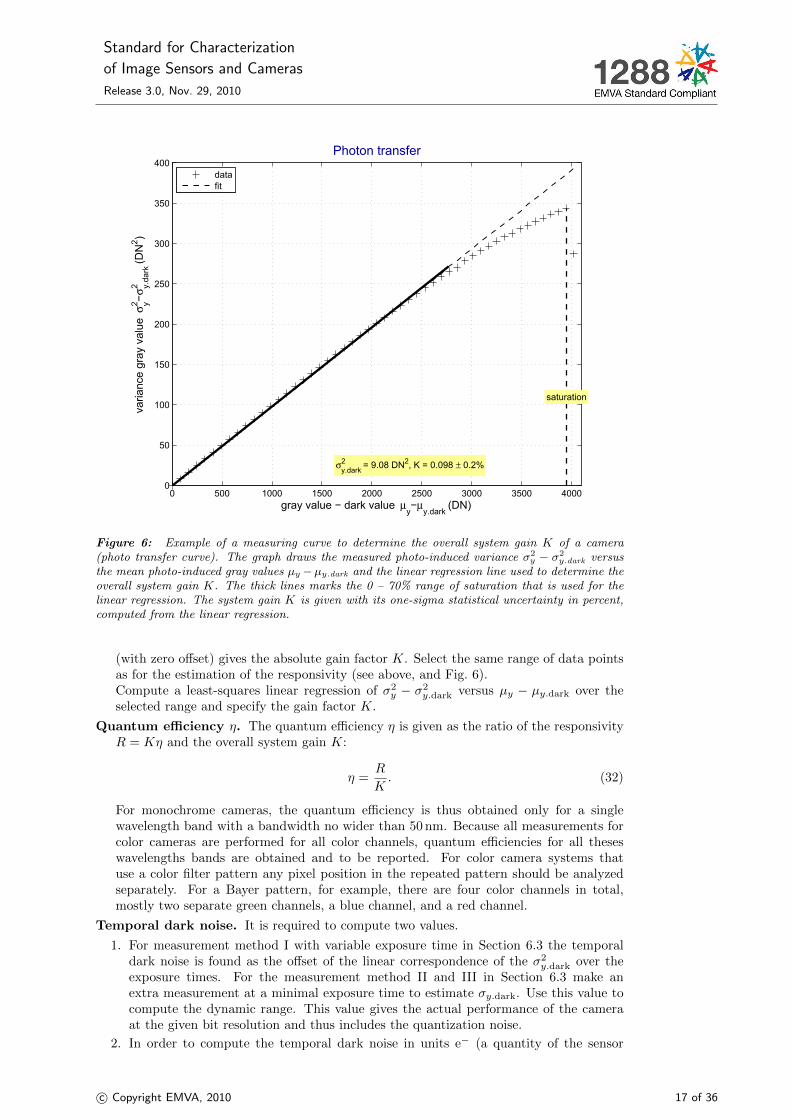
Figure 6: Example of a measuring curve to determine the overall system gain K of a camera(photo transfer curve). The graph draws the measured photo-induced variance σ2

y − σ2y.dark versus

the mean photo-induced gray values µy −µy.dark and the linear regression line used to determine theoverall system gain K. The thick lines marks the 0 – 70% range of saturation that is used for thelinear regression. The system gain K is given with its one-sigma statistical uncertainty in percent,computed from the linear regression.

(with zero offset) gives the absolute gain factor K. Select the same range of data pointsas for the estimation of the responsivity (see above, and Fig. 6).Compute a least-squares linear regression of σ2

y − σ2y.dark versus µy − µy.dark over the

selected range and specify the gain factor K.

Quantum efficiency η. The quantum efficiency η is given as the ratio of the responsivityR = Kη and the overall system gain K:

η =R

K. (32)

For monochrome cameras, the quantum efficiency is thus obtained only for a singlewavelength band with a bandwidth no wider than 50 nm. Because all measurements forcolor cameras are performed for all color channels, quantum efficiencies for all theseswavelengths bands are obtained and to be reported. For color camera systems thatuse a color filter pattern any pixel position in the repeated pattern should be analyzedseparately. For a Bayer pattern, for example, there are four color channels in total,mostly two separate green channels, a blue channel, and a red channel.

Temporal dark noise. It is required to compute two values.

1. For measurement method I with variable exposure time in Section 6.3 the temporaldark noise is found as the offset of the linear correspondence of the σ2

y.dark over theexposure times. For the measurement method II and III in Section 6.3 make anextra measurement at a minimal exposure time to estimate σy.dark. Use this value tocompute the dynamic range. This value gives the actual performance of the cameraat the given bit resolution and thus includes the quantization noise.

2. In order to compute the temporal dark noise in units e− (a quantity of the sensor




Release 3.0, Nov. 29, 2010

100 101 102 103 104 105 10610−1

100

101

102

103SNR


SN

R

satu

ratio

n

thre

shol

d S

NR

= 1

data fittheor. limit

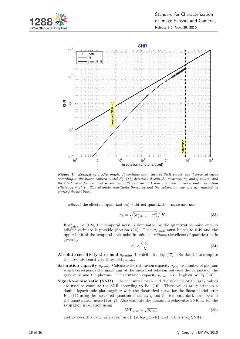
Figure 7: Example of a SNR graph. It contains the measured SNR values, the theoretical curveaccording to the linear camera model Eq. (11) determined with the measured σ2

d and η values, andthe SNR curve for an ideal sensor Eq. (13) with no dark and quantization noise and a quantumefficiency η of 1. The absolute sensitivity threshold and the saturation capacity are marked byvertical dashed lines.

without the effects of quantization), subtract quantization noise and use

σd =√

(σ2y.dark − σ2

q )/K. (33)

If σ2y.dark < 0.24, the temporal noise is dominated by the quantization noise and no

reliable estimate is possible (Section C.4). Then σy.dark must be set to 0.49 and theupper limit of the temporal dark noise in units e− without the effects of quantization isgiven by

σd <0.40

K. (34)

Absolute sensitivity threshold µp.min. Use definition Eq. (17) in Section 2.4 to computethe absolute sensitivity threshold µp.min.

Saturation capacity µp.sat. Calculate the saturation capacity µp.sat as number of photonswhich corresponds the maximum of the measured relation between the variance of thegray value and the photons. The saturation capacity µe.sat in e− is given by Eq. (14).

Signal-to-noise ratio (SNR). The measured mean and the variance of the gray valuesare used to compute the SNR according to Eq. (10). These values are plotted in adouble logarithmic plot together with the theoretical curve for the linear model afterEq. (11) using the measured quantum efficiency η and the temporal dark noise σd andthe quantization noise (Fig. 7). Also compute the maximum achievable SNRmax for thesaturation irradiation using

SNRmax =√µe.sat (35)

and express this value as a ratio, in dB (20 log10 SNR), and in bits (log2 SNR).




Release 3.0, Nov. 29, 2010

Dynamic range (DR). Use the definition Eq. (18) in Section 2.4 to compute the dynamicrange. It should be given as a ratio, in dB (20 log10 DR), and in bits (log2 DR).

6.7 Evaluation of Linearity

According to Section 6.5 at least 9 pairs of mean digital gray µy[i] and irradiation values H[i]are available. The linearity is determined by computing a least-squares linear regression withthe data points in the range between 5 and 95% of the saturation capacity µp.sat − µp.dark

y = a0 + a1H (36)

with an offset a0 and a slope a1 (Fig. 8a). Using this regression, the relative deviation fromthe regression can be computed by

δy[i] [%] = 100(µy[i]− µy.dark[i])− (a0 + a1H[i])

0.9(µy.sat − µy.dark), (37)

where µy.dark and µy.sat, are the dark and the saturation gray values, respectively (Fig. 8b).The factor 0.9 comes from the fact that only values in the range between 5 and 95% of thesaturation capacity µy.sat are considered. The linearity error is then defined as the mean ofthe difference of the maximal deviation to the minimal deviation

LE =max(δy)−min(δy)

2, (38)

and thus defines the mean of the positive and negative deviation from the linear regression.

7 Methods for Dark Current

7.1 Evaluation of Dark Current at One Temperature

Dark current measurements require no illumination source. From Eqs. (19) and (20) inSection 3 it is evident that the dark current can either be measured from the linear increaseof the mean or the variance of the dark gray value ydark with the exposure time. The preferredmethod is, of course, the measurement of the mean, because the mean can be estimated moreaccurately than the variance. If, however, the camera features a dark current compensation,the dark current must be estimated using the variance.

At least six equally spaced exposure times must be chosen. For low dark currents, itmight be required to choose much longer exposure times than for the sensitivity, linearity,and noise measurements.

The dark current is then given as the slope in the relation between the exposure timeand mean and/or variance of the dark value. A direct regression of the measured dark valuesgives the dark current in units DN/s. Use the measured gain K (units DN/e−) to expressthe dark current also in units e−/s.

If the camera’s exposure time cannot be set long enough to result in meaningful valuesfor the dark current, this value still must be reported together with its one-sigma error fromthe regression. In this way at least an upper limit of the dark current can be given, providedthat µI + σI > 0. The lower limit of the auto saturation time is then

tsat >µe.sat

µI + σI. (39)

7.2 Evaluation of Dark Current with Temperatures

The doubling temperature of the dark current is determined by measuring the dark currentas described above for different housing temperatures. The temperatures must vary over thewhole range of the operating temperature of the camera. Put a capped camera in a climateexposure cabinet or control its temperature in another suitable way and drive the housingtemperature to the desired value for the next measurement. For cameras with internaltemperature regulation and cooling of the image sensor no climate cabinet is required. Then




Release 3.0, Nov. 29, 2010

a

0 1 2 3 4 5 6 7 8 9

x 104

0

500

1000

1500

2000

2500

3000

3500

4000

Linearity


gray

val

ue −

dar

k va

lue

μy−μ

y.da

rk (D

N)

data fit

b

0 1 2 3 4 5 6 7 8 9

x 104

−1.4

−1.2

−1

−0.8

−0.6

−0.4

−0.2

0

0.2

0.4Deviation linearity


Line

arity

err

or L

E (%

)

LE = ± 0.41%

data

Figure 8: Example for the evaluation of the linearity: a Mean gray value minus the dark valueversus the irradiation plus the linear regression curve covering all measured values. The thick linesmarks the 5 – 95% range of saturation that is used for the linearity regression. b Percentage of thedeviation from the linear regression to determine the linearity error LE. The 5% and 95% saturationvalues are marked by dashed vertical lines, which range from min(δy) to max(δy), see Eqs. (37) and(38).




Release 3.0, Nov. 29, 2010

the temperature dependence of the dark current can only be measured in the temperaturerange that can be set.

After a temperature change wait until the camera values are stable. This is most easilydone by continuosly measuring the dark values at the largest exposure time. For eachtemperature, determine the dark current by taking a series of measurements with varyingexposure times as described in Section 7.1.

In order to determine the doubling temperature, the logarithm of the dark current mustbe plotted as a function of the temperature T . Then according to Eq. (21), a linear relationis obtained

log10 µI = log10 µI.ref + log10 2 · T − Tref

Td(40)

and the doubling temperature Td is given as the inverse slope a1 of a least-squares linearregression as log10 2/a1.

8 Methods for Spatial Nonuniformity and Defect Pixels

The measurements for spatial nonuniformity and the characterization of defect pixels areperformed with the same setup as the sensitivity, linearity, and noise, described in Section 6.Therefore, the basics measuring conditions are also the same (Section 6.5).

All quantities describing nonuniformities must be computed from mean gray valuesaveraged over many images. This is because the variance of the temporal noise (σy ≈ 1%) istypically larger than the variance of the spatial variations (sy ≈ 0.3− 0.5%). The temporalnoise can be suppressed by averaging over L images.

The typical figures imply that at least a sequence s of L = 16 images y are required sothat sy becomes large compared to σ2

y/L. This low value was chosen so that the methodcan also be applied for fast inline inspection. However, it is better to suppress the temporalnoise to such an extend that it no longer influences the standard deviation of the spatialnoise. This requires typically the averaging of L = 100−−400 images:

y′ =1

L

L−1∑l=0

s[l]. (41)

8.1 Spatial Standard Deviation, DSNU, PRNU

The measured variance when averaging L images is given by the sum of the spatial varianceand the residual variance of the temporal noise as

s2y.measured = s2

y + σ2y.stack/L. (42)

The spatial variance can be computed according to Eq. (42) by subtracting the temporalvariance:

s2y = s2

y.measured − σ2y.stack/L. (43)

The variance of the temporal noise must be computed directly from the same stack ofimages s[l] as the mean of the variance at every pixel using

σ2s[m][n] =

1

L− 1

L−1∑l=0

(s[l][m][n]− 1

L

L−1∑l=0

s[l][m][n]

)2

and σ2y.stack =

1

NM

N−1∑i=0

M−1∑j=0

σ2s[m][n].

(44)

The DSNU1288 and PRNU1288 values are then given according to Eq. (25) in Section 4.1 to

DSNU1288 = sy.dark/K (units e−),

PRNU1288 =

√s2y.50 − s2

y.dark

µy.50 − µy.dark· 100%.




Release 3.0, Nov. 29, 2010

a

0 0.05 0.1 0.15 0.2 0.25 0.3 0.35 0.4 0.45 0.510−1

100

101

102Horizontal spectrogram DSNU

cycles (periods/pixel)

stan

dard

dev

iatio

n (D

N)

sw = 1.50 DN, F = 1.98

b

0 0.05 0.1 0.15 0.2 0.25 0.3 0.35 0.4 0.45 0.510−1

100

101

102Vertical spectrogram DSNU


stan

dard

dev

iatio

n (D

N)

sw = 1.49 DN, F = 2.01

Figure 9: Example for spectrograms of the dark image: a Horizontal spectrogram b Verticalspectrogram. The dashed horizontal lines marks the white noise spectrum corresponding to thestandard deviation of the dark temporal noise σy.dark for acquiring a single image without averaging.




Release 3.0, Nov. 29, 2010

a

0 0.05 0.1 0.15 0.2 0.25 0.3 0.35 0.4 0.45 0.510−1

100

101

102Horizontal spectrogram PRNU


stan

dard

dev

iatio

n (%

)

sw = 0.54%, F = 1.02

b

0 0.05 0.1 0.15 0.2 0.25 0.3 0.35 0.4 0.45 0.510−1

100

101

102Vertical spectrogram PRNU


stan

dard

dev

iatio

n (%

)

sw = 0.54%, F = 1.02

Figure 10: Example for spectrograms of the photoresponse: a Horizontal spectrogram b Verticalspectrogram. The dashed horizontal lines marks the white noise spectrum corresponding to thestandard deviation of the temporal noise of the photoresponse in percent for acquiring a singleimage without averaging.




Release 3.0, Nov. 29, 2010

8.2 Horizontal and Vertical Spectrograms

The computation of the horizontal spectrograms requires the following computing steps:

1. Subtract the mean value from the image y.

2. Compute the Fourier transform of each row vector y[m]:

y[m][v] =1√N

N−1∑n=0

y[m][n] exp

(−2πinv

N

)for 0 ≤ v < N.. (45)

3. Compute the mean power spectrum p[v] averaged over all M row spectra:

p[v] =1

M

M∑m=0

y[m][v]y∗[m][v]− σ2y.stack/L, (46)

where the superscript ∗ denotes the complex conjugate and again the residual temporalnoise remaining — due to the averaging over only a finite number of L images — issubtracted. The power spectrum according to Eq. (46) is scaled in such a way thatwhite noise gets a flat spectrum with a mean value corresponding to the spatial variances2y.

In the spectrograms the square root of the power spectrum,√p[v], is displayed as a

function of the spatial frequency v/N (in units of cycles per pixel) up to v = N/2(Nyquist frequency). It is sufficient to draw only the first part of the power spectrumbecause the power spectrum has an even symmetry

p[N − v] = p[v] ∀v ∈ [1, N/2].

In these plots the level of the white noise corresponds directly to the standard deviationof the spatial white noise. Also draw a line with the standard deviation of the temporalwhite noise, σy (Figs. 9 and 10). In this way, it is easy to compare spatial and temporalnoise. Please note that the peak height in the spectrograms are not equal to the am-plitude of corresponding periodic patterns. The amplitude a of a periodic pattern canbe computed by adding up the spatial frequencies in the power spectrum belonging to apeak:

a = 2

(1

N

vmax∑vmin

p[v]

)1/2

. (47)

For the vertical spectrograms (area cameras only), the same computations are performed(Fig. 9b and Fig. 10b). Only rows and columns must be interchanged.

4. The total spatial variance is the mean value of the power spectrum

DSNU: s2y =

1

N − 1

N−1∑v=1

p[v], PRNU: s2y =

1

N − 15

N−8∑v=8

p[v], (48)

excluding the first eight frequencies only for the PRNU.

5. The white noise part of the spatial variance, s2y.white, is then given by the median of the

power spectrum. The median value can easily be computed by sorting the N values inthe vector p is ascending order to give a new vector psorted. The median is then thevalue at the position, psorted[N/2].

6. Finally, the non-whiteness factor F is computed as the ratio of the spatial variance andthe white-noise spatial variance:

F = s2y

/s2y.white (49)




Release 3.0, Nov. 29, 2010

8.3 Defect Pixel Characterization

Before evaluation of the PRNU image y′ = y50−ydark, this image must be highpass-filteredas detailed in Section 4.4 and Appendix C.5. No highpass-filtering is performed with theDSNU image ydark.

The computation of the logarithmic histogram involves the following computing stepsfor every averaged and highpass-fitered nonuniformity image y:

1. Compute minimum and maximum values ymin and ymax.

2. Part the interval between the minimum and maximum values into at least Q = 256 binsof equal width

3. Compute a histogram with all values of the image using these bins. The bin q to beincremented for a value y is

q = floor

(Q

y − ymin

ymax − ymin

). (50)

The values of the center of the bins as a deviation from the mean value are given as:

4. Draw the histogram in a semilogarithmic plot. Use a x-axis with the values of the binsrelative to the mean value. The y axis must start below 1 so that single outlying pixelscan be observed.

5. Add the normal propability density distribution corresponding to the non-white variances2nw as a dashed line to the graph:

pnormal[q] =ymax − ymin

Q· NM√

2π snw· exp

(− y[q]2

2s2nw

), (51)

where y[q] is given by inverting Eq. (50) as the y value in the middle of the bins:

y[q] = ymin +q + 0.5

Q· (ymax − ymin). (52)

The accumulated logarithmic histogram gives the probability distribution (integral ofthe probability density function) of the absolute deviation from the mean value. Thus theaccumulated logarithmic histogram gives the number of pixels that show at least a certainabsolute deviation from the mean in relation to the absolute deviation. The computationinvolves the following steps:

1. Subtract the mean from the averaged and highpass-fitered nonuniformity image y andtake the absolute value:

y′ = |y − µy| (53)

2. Compute the maximum value y′max of y′; the minimum is zero.

3. Part the interval between the zero and the maximum value into at least Q = 256 bins ofequal width

4. Compute a histogram with all values of the image using these bins. The bin q to beincremented for a value y is

q = floor(Qy′

y′max

). (54)

5. Accumulate the histogram. If h[q′] are the Q values of the histogram, then the values ofthe accumulated histogram H[q] are:

H[q] =

Q∑q′=q

h[q′]. (55)

6. Draw the accumulated histogram in a semilogarithmic plot. Use a x-axis with the valuesof the bins relative to the mean value. The y axis must start below 1 so that singleoutlying pixels can be observed.

Logarithmic histograms and accumulated logarithmic histograms are computed anddrawn for both the DSNU and the PRNU. This gives four graphs in total as shown inFigs. 11 and 12.




Release 3.0, Nov. 29, 2010

a

−10 −5 0 5 10 15 2010−1

100

101

102

103

104Logarithmic histogram DSNU

Deviation from mean (DN)

Num

ber o

f pix

el/b

in

snw = 2.11 DN

data fit

b

−25 −20 −15 −10 −5 0 5 1010−1

100

101

102

103

104

105Logarithmic histogram PRNU

Deviation from mean (%)

Num

ber o

f pix

el/b

in

snw = 0.55%

data fit

Figure 11: Example for logarithmic histograms for a dark signal nonuniformity (DSNU), b pho-toresponse nonuniformity (PRNU). The dashed line is the model normal probability density distri-bution with the non-white standard deviation snw according to Eq. (51).




Release 3.0, Nov. 29, 2010

a

0 2 4 6 8 10 12 14 16 18 20

10−3

10−2

10−1

100

101

102Accumulated log histogram DSNU

Deviation from mean (DN)

Per

cent

age

of p

ixel

/bin

b

0 5 10 15 20 25

10−3

10−2

10−1

100

101

102Accumulated log histogram PRNU

Deviation from mean (%)

Per

cent

age

of p

ixel

/bin

Figure 12: Example for accumulated logarithmic histograms for a dark signal nonuniformity(DSNU), b photoresponse nonuniformity (PRNU).




Release 3.0, Nov. 29, 2010

9 Methods for Spectral Sensitivity

9.1 Spectral Light Source Setup

The measurement of the spectral dependence of the quantum efficiency requires a separateexperimental setup with a light source that can be scanned over a certain wavelength range.This apparatus includes either a monochromator with a broadband light source or a lightsource that can be switched between different wavelengths by any other means. Use anappropriate optical setup to ensure that the light source has the same geometrical propertiesas detailed in Section 6.1. This means that a light source with a diameter D must evenlyilluminate the sensor array or calibration photodiode placed at a distance d = 8D witha diameter D′ ≤ D. A different aperture d/D can be used and must be reported. It isadvantageous to set up the whole system in such a way that the photon irradiance is aboutthe same for all wavelengths.

Spectroscopic measurements are much quite demanding. It might not be possible toilluminate the whole sensors evenly. Therefore only a section of the sensor may be used forthe spectroscopic measurements.

9.2 Measuring Conditions

This section summarizes the measuring conditions.

Sensor area. Specify the fraction of the sensor area used (all, half, . . . ).

Operation point. The operation point must be the same as for all other measurements.

Bandwidth. The FWHM (full width at half maximum) bandwidth of the light source shallbe less than 10 nm. If it is technically not feasible to work with such narrow FWHM,the FWHM bandwidth can be enlarged to values up to 50 nm. The FWHM used for themeasurement must be reported. Please not that if you use a FWHM larger than 10 nmit will not be possible to evaluate the color rendition of a color sensor, e. g., accordingto the ISO 13655 and CIE 15.2. Some image sensors show significant oscillations inthe quantum efficiency as a function of the wavelength of the light (Fig. 13). If suchoscillations occur, the peak positions vary from sensor to sensor. Therefore it is allowedto smooth, provided that the filter procedure is described including the width of thefilter.

Wavelength range. The scanned wavelength range should cover all wavelength to whichthe sensor responds. Normally, this includes a wavelength range from at least 350 nm to1100 nm. For UV sensitive sensors the wavelength range must be extended to correspond-ingly shorter wavelengths, typically down to 200 nm. If technically feasible, the numberof measuring points must be chosen in such a way that the whole wavelength range iscovered without gaps. This implies that the distance between neighboring wavelengthsis smaller than or equal to the 2 FWHM.

Signal range. An exposure time should be set to a value so that sufficiently large signals areobtained for all wavelengths. If the irradiation of the light source shows large variationsfor different wavelengths, this could require more than one spectral scan with differentexposure times. Before and after each wavelength sweep and for every exposure timeused, a dark image must be taken.

9.3 Calibration

The experimental setup is calibrated in the same way as the monochromatic setup (Sec-tion 6.4). The image sensor is replaced by a calibrated photodiode for these measurements.From the measured irradiance at the sensor surface, the number of photons µp(λ) collectedduring the exposure time are computed using Eq. (2).

9.4 Evaluation

The measured wavelength dependent quantum efficiency is averaged over all pixels of thesensor or the selected sensor area. For color cameras, the spectral response must be evaluatedfor all colors separately just in the same way as described at the end of Section 6.6.




Release 3.0, Nov. 29, 2010

300 400 500 600 700 800 900 1000 11000

0.05

0.1

0.15

0.2

0.25

0.3

0.35

wavelength λ (nm)

quan

tum

effi

cien

cy η

m1001, 08.02.2010

Figure 13: Example for a spectroscopic measurement of the quantum efficiency in a range from300–1100 nm with a FWHM of 7 nm, no smoothing is applied.

The evaluation procedure contains the following steps for every chosen wavelength:

1. Compute the mean spectral gray value.

2. Subtract the mean dark value from the mean spectral values.

3. Divide byK, as determined from the linearity and sensitivity measurements (Section 6.6),performed at the same operation point, to compute the number of accumulated chargeunits.

4. Divide by the mean number of photons, µp(λ), calculated using the spectral calibrationcurve Section 9.3 to obtain the quantum efficiency:

η(λ) =µy(λ)− µy.dark

K µp(λ). (56)

An example curve is shown in Fig. 13.

10 Publishing the Results

This section describes the basic information which must be published for each camera andprecedes the EMVA 1288 data.




Release 3.0, Nov. 29, 2010

10.1 Basic Information

Item Description

Vendor Name

Model Name

Type of data presented1 Single; typical; guaranteed; guaranteed over life time

Sensor type CCD, CMOS, CID, . . .

Sensor diagonal in [mm] (Sensor length in the case of line sensors)

Lens category Indication of lens category required [inch]

Resolution Resolution of the sensor’s active area: width x height in [pixels]

Pixel size width x height in [µm]

CCD only

Readout type progressive scan or interlaced

Transfer type interline transfer, frame transfer, full frame transfer, frame in-terline transfer

CMOS only

Shutter type Global: all pixels start exposing and stop exposing at the sametime. Rolling: exposure starts line by line with a slight delaybetween line starts; the exposure time for each line is the same.Other: defined in the data-sheet.

Overlap capabilities Overlapping: readout of frame n and exposure of frame n+1can happen at the same time. Non-overlapping: readout offrame n and exposure of frame n+1 can only happen sequen-tially. Other: defined in the data-sheet.

Maximum readout rate at the given operation point (no change of settings permitted)

Dark current compensation Specify whether camera has dark current compensation

Interface type Analog2, USB2, IEEE 1394a or b, CameraLink, . . .

Operation point(s) Describe operation points used for EMVA 1288 measurements(including gain, offset, maximum exposure time, mode of cam-era, . . . )

EMVA 1288 Specify which optional EMVA 1288 data have been measured1Specify definition used for typical data, e. g., number of samples, sample selection. The type of data may

vary for different parameters, e. g., guaranteed specification for most of the parameters and typical data for

some measurements not easily done in production. It then has to be clearly indicated which data is of what

nature.2 Specify frame grabber used with analog camera

10.2 The EMVA 1288 Parameters

The EMVA 1288 parameters should be published in the following way: A summary sheetwith a maximum of two pages should include

• The basic information about the camera as described in Section 10.1

• A table with all quantities according to Table 2, which are detailed in Sections 6–9.Quantities that are not mandatory according to Table 2 must be listed as well to makeclear what has not been measured.

• A graph with the photon transfer curve (Fig. 6)

• A graph with the SNR curve (Fig. 7)

• If spectrometric measurements are performed, a graph with the wavelength dependencyof the quantum efficiency (Fig. 13)

10.3 The EMVA 1288 Datasheet

This two-page summary sheet is followed by several pages with all the graphs that detailthe performed measurements and that are contained in Sections 6–9.




Release 3.0, Nov. 29, 2010

Table 2: List of all EMVA 1288 parameters with classification into mandatory and optional.

Type of measurement Mandatory Reference

Quantum efficiency η Y Specify center and FWHM wavelengths ofthe light source used

Gain 1/K Y units e−/DN

Dark noise Y in units DN and e−

DSNU1288 Y in units DN and e−

Signal to noise ratio SNRmax Y as ratio and in units dB and bits

SNR−1max Y in %

PRNU1288 Y in %

Non-whiteness factor F (dark) Y

Non-whiteness factor F (50%) Y

Non-linearity error LE Y %

Absolute sensitivity threshold Y in number of electrons and photons, specifycenter wavelength

Saturation capacity Y in number of electrons and photons, specifycenter wavelength

Dynamic range (DR) Y as ratio and in units dB and bits

Dark current Y in units DN/s and e−/s

Doubling temperature Td (K) N see Section 7.2

10.4 Template Datasheet

Two template datasheets, one for a monochrome camera, and one for a color camera, arepublished in extra documents. These template data sheets also detail all the axes labeling,and it is marked which graphs are mandatory.

A Bibliography

[1] Denvir, D. J. and E. Conroy. Electron multiplying CCDs. In Shearer, A., F. D. Murtagh,J. Mahon, and P. F. Whelan, eds., Optical Metrology, Imaging, and Machine Vision, vol. 4877of SPIE Proc., pp. 55–68, 2003.

[2] DeWeert, M. J., J. B. Cole, A. W. Sparks, and A. Acker. Photon transfer methods andresults for electron multiplication CCDs. In Tescher, A. G., ed., Applications of Digital ImageProcessing XXVII, vol. 5558 of SPIE Proc., pp. 248–259, 2004.

[3] Dierks, F. Sensitivity and Image Quality of Digital Cameras. http://www.baslerweb.com.

[4] Holst, G. C. and T. S. Lomheim. CMOS/CCD Sensors and Camera Systems. SPIE, 2007.

[5] Janesick, J. R. Scientific Charge-Coupled Devices. SPIE, Bellingham, WA, 2001.

[6] Janesick, J. R. CCD characterization using the photon transfer technique. In Prettyjohns, K.and E. Derenlak, eds., Solid State Imaging Arrays, vol. 570 of SPIE Proc., pp. 7–19, 1985.

[7] Janesick, J. R. Photon Transfer. SPIE Press, 2007.

[8] Jahne, B. Digital Image Processing. Springer, Berlin, 6th edn., 2005.

[9] Labsphere. A Guide to Integrating Sphere Theory and Applications. Technical guide, seehttp://www.labsphere.com/, 2003.

[10] Labsphere. Integrating Sphere Uniform Light Source Applications. Technical guide, seehttp://www.labsphere.com/, 2003.

[11] Theuwissen, A. J. P. Solid-State Imaging with Charge-Coupled Devices. Kluwer AcademicPublishers, 1995.

[12] Widrow, B. and I. Kollar. Quantization Noise — Roundoff Error in Digital Compu-tation, Signal Processing, Control, and Communications. Cambridge Univ Press, 2008.www.cambridge.org/9780521886710.


http://www.baslerweb.com

www.cambridge.org/9780521886710



Release 3.0, Nov. 29, 2010

B Notation

This section summarizes the used notation in two tables. The first table describes all quan-tities used, the second table, the meaning of indices that are used with various quantities.With this split in the description, the notation tables are much shorter.

Quantity Units Description

A µm2 Area of a sensor element (pixel)

c m/s Velocity of light

d mm Distance of sensor plane to opening (aperture) oflight source

D mm Diameter of opening (aperture) of light source

D′ mm Diameter of image sensor

DSNU1288 DN Dark signal nonuniformity

DR 1, dB, bits Dynamic range

E W/m2, Photons/(s pixel) Irradiance at sensor plane

F 1 Non-whiteness factor, def. Eq. (49)

h Js Planck constant

H Ws/m2, Photons/pixel Irradiation (exposure) at sensor plane

k m−1 wave number

K DN/e− Overall system gain of a digital camera

PRNU1288 % Photo response nonuniformity

SNR 1, dB, bits Signal to noise ratio

p — Power spectrum

s — spatial standard deviation of the quantity putinto the index

s2 — spatial variance of the quantity put into the index

s DN Digital image sequence

texp s Exposure time

y DN Digital gray value

y DN 2-D digital image

η 1 Total quantum efficiency, def. Eq. (1)

λ nm wavelength of light

µ — mean of the quantity put into the index

ν Hz frequency of light

σ — temporal standard deviation of the quantity putinto the index

σ2 — temporal variance of the quantity put into theindex

Index Units Description

d e− relates to dark signal in units of e−

dark DN relates to dark signal in units of DN

e — relates to number of electrons

min — relates to absolute sensitivity threshold

p — relates to number of photons

q — relates to quantization noise

sat — relates to saturation of the sensor

[l] — selection of an image in a image sequence

[m] — selection of a row in a image

[n] — selection of a column in a image




Release 3.0, Nov. 29, 2010

C Changes to Release A2.01

This section summarizes the changes of release 3.0 over the previous release A2.01 of theEMVA 1288 standard. Mostly, only extensions were added to the standard as describedin Section C.1. To improve the standard and simplify its usage some minor changes werenecessary. All these changes were implemented in release 3.0 in a way so that the data ofcameras measured according to the specifications of release A2.01 are still valid.

C.1 Added Features

The following features are added to release 3.0 of the standard:

1. Color sensors and color cameras and not only gray scale cameras are now covered

2. Flexible characterization of defect pixels via logarithmic histograms (Sections 4.3 and 8)

C.2 Extension of Methods to Vary Irradiation

In release A2.01 of the standard, the photon transfer method (sensitivity and noise mea-surements) had to performed with a continuous light source and varying exposure times,while the linearity measurements had to be measured with a constant exposure time and apulsed light source with varying pulse widths. This was awkward, because the same type ofmeasurements had to be performed twice.

With release 3.0 of the standard, any method described in Section 6.3 can be used tovary the irradiation and so the same set of measurements can be used to evaluate the dataaccording to the photon transfer method (Section 6.6) and to determine the linearity error(Section 6).

C.3 Modifications in Conditions and Procedures

The following measuring conditions have been unified, described more precisely, or beenchanged:

1. For the photon transfer method, the mean value has to be computed from both imagesaccording to Eq. (30), and not only from the first as in release A2.01.

2. Condition to set the offset of the camera in order to avoid underflow with linearitymeasurements and nonuniformity measurements (Section 6.5). In release A2.01 differentconditions were prescribed for linearity measurements, photo transfer measurements, andnonuniformity measurements.

3. The number of measuring points for sensitivity, linearity, and noise measurements isincreased to 50. Only for production measurements as few as 9 values are allowed.

4. Number of images to be used for nonuniformity measurements. It is now possible toperform these measurements with just 16 images for inline inspection by correcting thebias caused by the residual temporal noise (Section 8).

5. The spatial noise is no longer contained in the definition of the SNR (compare Eq. (11)with Eq. 15 of release A2.01. This change has been made, because it is possible to reducethe spatial nonuniformities by suitable shading correction techniques with a single image,while this is not possible with the temporal noise.

6. The condition for the gray value range for the regression of the mean gray values againstthe irradiation has been better adapted to possible nonlinearities in this relation. Inrelease A2.01 it was at least the range from the dark image to 80% of the maximumtemporal variance (Section 6.6), now it is reduced to 70%.

7. For a computation of the absolute sensitivity threshold the more accurate equationEq. (17) is used. This change was required because the old equation without the correc-tion term 1/2 in release A2.01 is not accurate enough for cameras with a very low darknoise of only a few electrons.

8. The linearity LE must be specified for the interval of 5–95% of the saturation points(Section 6.7).




Release 3.0, Nov. 29, 2010

a

0.3 0.4 0.5 0.6 0.7 0.8 0.9 10

0.01

0.02

0.03

0.04

0.05

0.06Estimation of mean values

Standard deviation temporal noise [DN]

Est

imat

ion

erro

r [D

N]

standard deviation errormaximal error

b

0.3 0.4 0.5 0.6 0.7 0.8 0.9 1−0.2

−0.15

−0.1

−0.05

0

0.05

0.1

0.15Estimation of standard deviation

Standard deviation temporal noise [DN]

Est

imat

ion

erro

r [D

N]

minmaxmean

Figure 14: Results from Monte Carlo simulations for the estimation of a the mean value and bthe standard deviation of the digital gray value as a function of the standard deviation in units ofdigital numbers [DN] in the range between 0 and 1.

9. For dark current measurements a minimum number of six equally spaced exposure timesmust be used (Section 7.1).

10. For a proper analysis of defect pixels, a highpass filtering is introduced so that the PRNUmeasurements are not spoiled by the imperfections of the used light source (Section 4.4).This highpass filtering is used also before all other nonuniformity evaluations includ-ing the estimation of spatial variances (Section 8.1) except for the computation of thespectrograms and all quantities derived from them (Section 8.2).

11. Measuring conditions for spectral measurements are relaxed (Section 9). The f -numbercan now deviate from 8, but must be reported.

C.4 Limit for Minimal Temporal Standard Deviation; Introduction of QuantizationNoise

In the previous releases of the standard, quantization noise was neglected in the linearcamera model. This led to a more complicated measuring procedure with low-resolutiondigitalization, i. e., 8 bit cameras. The problem resulted from the fact that the standarddeviation of the temporal noise in the dark image may become smaller than the quantizationinterval.

Versions 1 and 2 of the EMVA 1288 standard therefore recommended:

”The gain setting of the camera is as small as possible but large enough to ensure thatin darkness

Kσd ≥ 1

holds true (Otherwise, the quantization noise will spoil the measurement.)”

It turns out that this limit is too cautious [12]. Monte-Carlo simulations were performedto check how accurate the mean and the variance can be estimated as a function of standarddeviation σy in units DN. For the simulations 201 mean gray values equally distributedbetween 0 and 1 were taken and zero-mean normally distributed noise was added to thevalues. The estimated mean and variances were averaged over 900 000 realizations of eachvalue. Finally, the deviations in the estimations were averaged over all 201 values.

The results are shown in the range [0.3, 1] for σy in Fig. 14. The mean gray value canbe estimated with a maximum error of less than 0.014 DN even for standard deviations aslow as 0.4 DN (Fig. 14b). The estimate of the standard deviation is biased by the addi-tional standard deviation of the quantization, σq =

√1/12. However, if the estimate of

the standard deviation is corrected for the additional effect of the standard deviation of thequantization error (unbiased estimation)

σ2y = σ2

est − σ2q = σ2

est − 1/12, (57)




Release 3.0, Nov. 29, 2010

the maximum error of the estimate remains below 0.04 even for standard deviations as lowas 0.4. The variation in the estimation of the standard deviation comes from the differentpositions of the mean in the [0, 1] interval. If it is close the edge of the interval, the valuesflip often either to the higher or lower value, resulting in a higher standard deviation. Ifthe mean is in the middle of the interval this happens less frequently, so that the standarddeviation is lower.

In conclusion, the variance σ2y.dark must be larger than 0.24 DN2. Subtraction the quanti-

zation noise variance σ2q = 1/12 DN2, this results in a minimal detectable temporal standard

deviation of 0.40 DN. If the measured temporal variance is smaller than 0.24 DN2, two thingscan be stated:

1. The dynamic range is limited by the quantization noise (and the maximum possible butnot determinable temporal noise to µy.sat/0.49.

2. The standard deviation of the dark noise in units e− can be estimated to σd < 0.40/K.

The correction of the temporal noise by the quantization noise, which is possible downto a measured temporal noise variance of 0.24, expands the measurable dynamic range of acamera by a factor of about 2 over the condition of release A2.01. For a 8-bit camera, themaximum and measurable dynamic range is 255/0.49 ≈ 500

C.5 Highpass Filtering with Nonuniformity Measurements

The highpass filtering with defect pixel measurements is implemented by subtracting a 5× 5box-filtered image from the original mean images:

y′ = y − 5R ∗ y with 5R =

1 1 1 1 1

1 1 1 1 1

1 1 1 1 1

1 1 1 1 1

1 1 1 1 1

/25. (58)

The transfer function of this highpass filter is given by [8, p. 303]:

ph(k1, k2) = 1− sin(πP k1/2)

P sin(πk1/2)· sin(πP k2/2)

P sin(πk2/2), (59)

where P = 5 and k1 and k2 are the wave numbers in horizontal and vertical direction,respectively, normalized by the spatial Nyquist frequency. This type of highpass filteringremoves only a small fraction of the white noise. This can be computed by integrating overthe squared transfer function

s2y′ = s2

y

1∫k1=0

1∫k2=0

r2(k1, k2) dk1dk2 = s2y(1− r0,0)2 = s2

y

(1− 1

P 2

)2

= 0.92 s2y, (60)

provided that the spectrum of the random spatial variations is white (Section 4.2). Thusthis method efficiently suppresses low-frequency spatial variations of the light source withoutreducing the estimate of the variance of the white noise significantly. For the proposed 5× 5box filter (P = 5), the reduction in the standard deviation is just 4%: σy′ = 0.96σy.Therefore the measured spatial standard deviation sy′ must be divided by 0.96 in order toobtain the correct value sy.

For all further processing leave out two border lines at the top and bottom and twoborder columns on the left and right of the filtered image, because the filtering will not beexact in these areas. This procedure reduces the image size by four lines and four rows.

For line-scan cameras only a horizontal 5× 1 box filter is applied. Therefore the correc-tion factor is in this case (compare Eq. (60))

s2y′ = s2

y

1∫k1=0

r2(k1) dk1 = s2y(1− r0)2 = s2

y

(1− 1

P

)2

= 0.64 s2y. (61)




Release 3.0, Nov. 29, 2010

The measured spatial standard deviation for line cameras sy′ must be divided by 0.80 in orderto obtain the correct value sy. For all further processing of highpassed average nonuniformityimages from line cameras leave out two border columns on the left and right.


emva standard 1288 - zenodo.org

Documents