1

DRAFT – NOT FOR CITATION

The findings, interpretation and conclusions expressed in this paper are entirely those of the authors. They do not necessarily represent the views of The World Bank and its affiliated organizations, or those of the Executive Directors of the World Bank or the governments they represent. If you wish to comment on this paper, please send your comments to Priya Shyamsundar (pshyamsundar@worldbank.org) or Sushenjit Bandyopadhyay (sbandyopadhyay@worldbank.org)

Yield Impact of Irrigation Management Transfer: A Success

Story from the Philippines

Sushenjit Bandyopadhyay*, Priya Shyamsundar*

*Affiliations: The World Bank

Addresses:

Environment Department - The World Bank

1818, H Street, NW - Mail Stop MC5-511

Washington DC - 20433 – USA

Corresponding Author:

Sushenjit Bandyopadhyay

Environment Department - The World Bank

1818, H Street, NW - Mail Stop MC5-511

Washington DC - 20433 – USA

sbandyopadhyay@worldbank.org

Ph: +1 202 473 7690

2

Abstract

Irrigation Management Transfer (IMT) is an important strategy among donors and governments

to strengthen farmer control over water and irrigation infrastructure. In this study, we seek to

understand if IMT is meeting the promise of its commitments. We use data from a survey of 68

irrigator associations and 1020 farm households in the Philippines to estimate the impact of IMT

on irrigation association performance and on rice yields. We also estimate a stochastic frontier

production function to assess contributions to technical efficiency. We find that: a) IMT

contributes to an increase in maintenance activities undertaken by irrigation associations. While

associations with and without IMT contracts undertake canal maintenance, the frequency of

maintenance in IMT IAs is higher; b) by increasing local control over water delivery, IMT

increases farm yields by 2-6%. Rice production in IMT areas is higher even after we control for

various differences amongst rice farmers in IMT and non-IMT areas; and, c) IMT is, at a

minimum, poverty-neutral, and may even give the asset-poor a small boost in terms of rice yields.

We speculate that this boost may be a result of increased timeliness of water delivery and better

resolution of conflicts related to illegal use.

Key words: Irrigation Management Transfer, Stochastic Production Function, Impact

Evaluation, the Philippines.

3

Yield Impact of Irrigation Management Transfer: A Success

Story from the Philippines

1. Introduction

Over the last several decades communities have increasingly sought and won control over

the management of natural resources. Developing countries have seen a shift from

traditional state control over resources to increased local authority. This trend towards

decentralization in resource management is a result of a growing recognition that the state

cannot effectively monitor the local uses of natural resources. Simultaneously, it has also

become clear that the local communities, under differing circumstances and conditions,

are able to cooperate to successfully manage resource use (Ostrom 1990, Baland and

Platteau 1996, Agrawal 2001).

While decentralization in resource management is prevalent in several sectors, it is

perhaps strongest in irrigation management. This process of transferring irrigation

management responsibilities from the government to farmer or irrigator organizations,

also known as irrigation management transfer (IMT), first began and expanded in the

United States, France, Colombia, and Taiwan during the 1950s through the 1970s. Many

developing countries followed this trend in the 1980s and 1990s (Vermillion 1992, Araral

2005). Today, participatory irrigation is an important component of irrigation reform

worldwide.

4

There are many reasons for the increased interest in participatory irrigation. First,

irrigation provision has proven to be a large financial burden on national irrigation

agencies and exchequers. Cash-strapped irrigation departments, unable to sustain

investments in infrastructure, are looking to transfer operational responsibilities to

farmers. Further, the possibility of increased floods and droughts from climate change has

re-focused attention on water-use efficiency and the need for local scrutiny and control.

Third, there is a general trend towards all forms of decentralization in government

functions, which has found support in the irrigation sector as well.

In practical terms, participatory irrigation has meant a reduced role for government

agencies in operation and maintenance (O&M), fee collection, water management, and

conflict resolution. It has also resulted in the growth of a larger number of farmer-run

irrigation or water user associations. These farmer associations have taken on numerous

functions that were previously the responsibility of national irrigation agencies.

While participatory irrigation management is widespread, there is surprisingly little

evidence about its impacts (Araral 2005). While many studies focus on government

savings, fewer have sought to quantify impacts on farm productivity or water

conservation (see Araral 2005 and Vermillion 1997). A recent exception is a study by

Wang et al. (2006), which examines the role of water user associations in influencing

water savings in China. They find that monetary incentives to water managers can

5

contribute to water savings; however, these savings do not result in any increase in the

incidence of poverty.

An increasingly loud criticism is that with its focus on the state’s financial burdens,

irrigation reform has moved away for its original objectives of improving the livelihoods

of poor farmers (Kloezen et al. 1997; Vermillion 1997; Koppen et al. 2002; Shah et al.

2002). The majority of the world’s poor is rural and dependent on farming in one form or

the other. Thus, institutional reform in the irrigation sector ultimately has to contribute to

the lot of the poor. Thus, far there are few studies that carefully examine this question.

There is also little empirical literature on whether there are differential effects of

institutional reforms within farming communities.

Given the many gaps in the literature on irrigation management transfer, this paper is

motivated by the need to understand the farm level impacts of irrigation management

transfer. The paper seeks to answer three questions: a) does irrigation management

transfer result in improvements in the irrigation system through increased operations and

maintenance and better revenue collection? b) Does the increased control farmers have as

a result of IMT translate to improvements in crop yield? And c) do these improvements

differ for rich and poor farmers? We address these questions in the context of a case

study in the Philippines.

We primarily use an econometric approach to answer these questions. We first examine

whether the performance of irrigation associations as reflected in operations and

6

maintenance activities changes when management transfer occurs. The hypothesis is that

management transfer leads to local control and improves system performance. Second,

we look at farm yield impacts. We estimate a Cobb-Douglas production function and

examine whether yields are affected by increased local control over water delivery. Third,

we estimate a stochastic frontier production function to assess the decrease in overall

production in-efficiency. We then look at distributional issues related to yield impacts to

understand whether irrigation reforms have a similar effect on rich and poor farmers.

This paper is based on data from a survey of 1020 households and 68 irrigation

associations covering the Magat River Integrated Irrigation System, a reservoir irrigation

system in the Philippines. The section below first describes the irrigation management

system in the Philippines. This is followed by a discussion on methodological issues and

data. Results and conclusions follow.

2. Irrigation Management Transfer in the Philippines

In the Philippines, approximately 1.4 million hectares of land is irrigated. Fifty percent

of this area is managed publicly under national irrigation systems; some 37% is managed

by communal irrigation systems and 13% by private irrigation systems. The national

systems are owned and operated by the National Irrigation Administration (NIA), a semi-

autonomous government corporation that is responsible for irrigation development.

(Sabio and Mendoza 2002, Bagadion 2002).

7

The Philippines history of organizing farmers to improve production goes back to the late

sixties. However, a more participatory approach to irrigation management was first

developed in the mid-1970s for communal systems, and then expanded to national

systems in the 1980s. By December 1999, some 2078 IAs operated in nationally owned

irrigation systems and 3018 IAs managed communal systems. Overall, these irrigator

associations cover 82% of the area developed for irrigation (Mejia 2002).

The late nineties saw the emergence of a new type of contractual relationship between

irrigation associations and the National Irrigation Agency in the form of irrigation

management transfer. This meant that NIA would progressively become a "whole-sale

irrigation water manager" for head-works and main systems, while empowered irrigators

associations took over responsibility for smaller systems. This strong push towards

decentralization effort was supported by two World Bank loans and resulted in a number

of irrigation associations with IMT contracts.1

A typical irrigation association has a Board of Directors and Officers. It oversees a

variety of irrigation management and infrastructure maintenance related tasks and in

some cases offers other services as well. NIA supports the growth and development of

these IAs, which can enter into different types of contracts with NIA. An IMT contract,

1 In December 1997, the Government enacted it’s the Agriculture and Fisheries Management Act, which

facilitated the decentralization in irrigation. IMT was supported with two World Bank loans under the

Second Irrigation Operations Support Project which was completed in 2000, and the Water Resources

Development Project.

8

in particular, transfers operations and maintenance responsibilities of secondary canals to

IAs in large systems and O&M of the entire system in case of smaller systems (3000

hectares or less) (World Bank 2001). This transfer in O&M responsibility is

accompanied by changes in how water-user fees are obtained from farmers and used by

associations. In most cases, the change marks a move to a simple 50-50 sharing of water

user fees between IAs and NIA – this money is collected by IAs from members and sent

to NIA, which then returns part of the fees.

The motivation behind IMT is that it will reduce government responsibilities for

operation and maintenance and simultaneously increase farmer supervision over water-

use. In general, irrigation management transfer is in line with a broad government

strategy to empower communities through decentralization, increase accountability and

quality of public sector services, and, streamline the public sector. This move, by

lowering government expenditures on irrigation and strengthening local governance, is

expected to have a long-term impact on the country’s agricultural and natural resource

sectors.

3. The Benefits of Irrigation Management Transfer

Irrigation management transfer can be expected to affect farm households through

multiple ways. The pathways through which the farm benefits occur are presented in

Figure 1.

9

First, IMT is expected to increase the control local farmer associations have on irrigation

infrastructure and water. For example in a recent survey of 63 IMT contracts in 19

systems across the Philippines provides, association leaders were asked what they liked

most about IMT -- the top two reasons were the sense of ownership and control and

access to revenues (Hassal and Associates International 2004). With an IMT contract,

these associations can make better decisions regarding water delivery and timeliness and

can organize themselves to resolve conflicts and maintain infrastructure. Without local

control, associations have to wait for the national agency to come in and undertake

repairs – with IMT they perform repairs as and when needed.

In terms of revenue generation, an IMT contract makes IAs responsible for collecting

user fees from members. The fees are remitted to the National Irrigation Agency, which

then sends back a portion. While this process of money transfer is tedious and has

resulted in many complaints about NIA, it still increases access to resources by IAs.

These resources are critical to the functioning of IAs and enable them to harness

members to undertake routine maintenance of canals.

Irrigation management transfer to the extent that it improves the quantity and timeliness

of water delivery and reduces uncertainty also affects farm yields. First, there is the

direct effect of having water when the farmer needs it. Crops require water at different

stages and yields are likely to improve if there is a good match between water delivery

and critical growth stages. Second, if the farmer is more certain about water delivery,

then this may affect his or her decisions related to other input use. Thus, it is likely to

10

increase the overall efficiency of farm production. This is an issue that we examine in

detail in this paper.

Also of interest to us in this paper is the distributional effect of institutional change.

Recent literature on decentralization in natural resource management raises the possibility

of elite capture, with the rich gaining more than the poor (Adhikari 2003; Klooster 2000a;

Klooster 2000b). In an interesting study, Koppen et al. (2002), compare the impacts of

irrigation management transfer on poor and non-poor farmers in India and note that

interests of the poor do not always overlap with the overall general goals of irrigation

schemes. They find that small farmers, who often participate in repair and rehabilitation

work, can be unaware of the existence of the water user association, while large farmers

involve themselves in committee work and makes decisions. The evidence from Andhra

Pradesh and Gujarat, India, points to the strong domination of local elite.

IMT increases local control over water-distribution and can result in localized re-

allocation of water – the effect of this on poorer farmers is not clear and will depend on

the type of re-allocation done. However, improved matching of farmer needs with water

availability could mean that there is more water available in upstream as well as

downstream areas. To the extent that the poorer households are located in downstream

areas, any improvements in water availability will give them an additional boost.

While the theory on how IMT is supposed to work is reasonably clear and there is some

evidence that IMT is beneficial, there are questions globally about whether governments

11

have been too fast in passing on irrigation management responsibilities to local

associations (Fujuiie et al. 2005). It is important to carefully examine if ground reality

matches the conceptual design of irrigation reforms in the Philippines. Clearly, there are

many things that are changed locally when institutional reforms are implemented. There

are several levels at which decisions need be made – NIA level, IA level as well as by the

farmer and at each stage there may be incentives that work to promote or undermine the

change. Thus, whether IMT is good for irrigation in the Philippines is an empirical

question and we examine various aspects of this question in the rest of the paper.

4. Study Area and Descriptive Statistics

Our study was undertaken in the Magat River Integrated Irrigation System (MRIIS) in

Region-2, Luzon, of the Philippines. The system is located in the basin of the Magat

River, which runs into the Cagayan Valley. It covers 85,294 hectares of service area and

encompasses three provinces: Isabella, Quirino and Ifugao.2 The dams in this system

provide year-round irrigation and rice is the major crop grown. Our goal was examine

one particular fairly simple reservoir-based irrigation system to understand whether IMT

was indeed beneficial to farmers.

Irrigation associations started in MRIIS more than two decades ago. Some of the earliest

IAs were registered in 1980 and the number of IAs rapidly expanded during the eighties.

2 It has four administrative irrigation districts: District III (20,366 hectares) is on the left bank of the river

and Districts I (21,797 hectares), II (23,241 hectares) and IV (19,890 hectares) on the right bank.

12

However, IAs with IMT contracts is a relatively new phenomenon. As of 2003 some

60% of the service area was under IMT contracts. For our study, we collected primary

data from 68 irrigation associations or approximately 20% of the 349 IAs in MRIIS. The

survey included questions on irrigation infrastructure, service fees, IA or CIA (council of

IAs) governance, and system O&M.

We selected a random sample of 43 IAs under IMT contract and 25 IAs that were not

under IMT for the survey. Our goal was to carefully examine the IAs with IMT contracts

and compare their performance with similar IAs that had yet to sign these contracts. Our

sample data shows that 86% of the selected IMT IAs had signed their IMT contract with

NIA prior to or during 2001. To the best of our understanding, as of 2006 all the IAs in

MRIIS had signed an IMT contract.

Our study also involved a household survey of 1020 farm households or approximately

9% of the total IA membership in MRIIS. The households selected for this study were

chosen from a master list of IA farmer members from the District Offices. A random

sample of 15 farmers was identified from each IA. The survey of IA and farm households

was undertaken during May to August of 2003. The survey collected data on various

farm level inputs and outputs as well as information on the effects of IMT. Secondary

data was obtained on variables such as historical user fee collection from the irrigation

district offices.

13

A simple comparison of IAs with IMT and IAs without IMT along different indicators is

presented in Table 1. It shows that both IMT and non-IMT IAs are of approximately the

same size in terms of hectares managed. The IMT IAs tend to service a somewhat larger

number of farmers and seem to have slightly greater percentage of upstream and

midstream farmers. In terms of irrigation infrastructure, the IMT IAs have a slightly

larger number of gates, more lined canals and modified infrastructure. These differences

are not huge and are logical because IAs tend to get some infrastructure assistance prior

to obtaining IMT contracts.

Interestingly there are few obvious differences amongst IMT and non-IMT IAs in terms

of a variety of governance indicators on which we collected data. For instance, there is

little difference in the fee collection rate from farmer members or number of female

Board members. However, we do find that IMT IAs are better at managing and resolving

conflicts from the household data. Households in IMT and non-IMT areas were asked

various questions about irrigation water distribution, conflicts and conflict resolution and

involvement in maintenance activities. Significantly more households in IMT IAs said

that the IAs helped with conflict resolution (see Table 2).

An important objective of transferring management responsibility to IAs is to enable

them to take over routine maintenance of irrigation infrastructure. A simple comparison

of means shows that this is true of some indicators. A larger percentage of IMT IAs are

likely to prepare maintenance plans each year and participate in canal cleaning. There

are other indicators of maintenance on which IMT and non-IMT IAs do equally well. A

14

significantly larger percentage of households in IMT areas relative to non-IMT areas said

that the water distribution schedule was followed and they participated in routine

maintenance activities (Table 2).

Simple mean differences between farm households are reported in Table 2, which shows

that about 84% of the sample of farmers has at least a high school degree and some 40%

of the households are college educated. There is little difference in education, household

assets or livestock between farmers in IMT and non-IMT areas. Farmers in both areas on

average farm approximately 2.4 hectares on land in each season. Thus, the average farm

is still rather small.

While household characteristics and assets are more or less equal among farmers in IMT

and non-IMT areas, there are some interesting differences in farm output. Farmers in

IMT areas have on average a 7% higher yield. In the next few sections we follow up on

this issue and ask if the higher yield can be attributed to the presence of IMT.

The survey also asked questions about perceptions of change over the last five years. As

Table 2 shows, a larger percentage of farmers in IMT areas said that they had seen

improvements in three aspects: a) services provided by IAs or NIA; b) participation of

farmers in O&M activities; and c) timeliness of water delivery. In general, the first level

analyses of mean differences among households in IMT and non-IMT IAs suggests that

households in IMT areas do better in terms of a variety of irrigation related issues.

15

5. Methods

We try to gauge whether or not IMT is successful is by examining IA performance and

by investigating farmer level benefits. There are many methodological challenges to

assessing performance and ascribing improvements to IMT, which we discuss below.

5.1. IMT impacts on irrigation association performance

The IMT contract hands over responsibility over canal O&M to IAs. It also specifies that

the IAS have to collect membership dues. But does this actually happen? And does it

translate to a greater effort at canal re-shaping or improved efficiency in fee collection?

Another methodologically important question is whether any observed differences are

due to IMT or other pre-existing factors. To answer such questions, we consider IAs

with IMT contracts and very similar IAs that have yet to sign their contracts and examine

their performance.

In order to attribute differences in IA performances to an IMT contract, we have to

account for pre-existing differences. A simple comparison of mean differences in

outcomes does not tell us whether this reflects IMT influence. In particular, some of the

pre-existing differences between IAs may have been instrumental to specific IAs being

selected for IMT. For example, IAs with more irrigation infrastructure are more likely to

join IMT. Similarly, IAs with leaders with better leadership skills may be more likely to

16

join in IMT. In both these cases the factors influencing the participation in IMT are also

factors that influence the performance of the IAs.

While various irrigation infrastructures are observable in our data, the leadership skills of

IAs leaders are not. These are examples of selection bias based on both observable and

unobservable data. Under ideal conditions, correction for both observable and

unobservable selection bias in the evaluation of impacts requires before and after

intervention data. Without base-line ‘before IMT’ data, we use cross-sectional data and

compute the average treatment on treated (ATT) by comparing IMT IAs with non-IMT

IAs using propensity score and instrumental variable techniques.

The treatment in the ATT is the participation of IAs in IMT and the treated refers to the

IMT-IAs. Thus, ATT measures the average effect of IMT on performance of those IAs

with IMT contrasted with the hypothetical scenario where these IAs did not have IMT.

We estimate ATT using both non-parametric and parametric methods. The non-

parametric estimators of ATT are based of propensity score matching.

A propensity score is an index that is based on the probability of an IA having an IMT

contract. It is used to match the non-IMT IAs (i.e. the comparator group) with IMT IAs

(i.e. the treatment group) on the basis of a set of observed characteristics. This method is

appealing where only cross-sectional data are available to examine program impacts and

is regarded as one of the best alternatives when random experiment design is not possible

(Rubin 1973).

17

To calculate the propensity score, we model the probability of an IA being selected for

IMT as a function of aggregated household and community characteristics.

)1()1Pr( 210 eIAFIMT +++Φ== ααα (1)

where IMT is an indicator variable that takes the value 1 if an IA is an IMT-IA and 0

otherwise. The probability of an IA becoming an IMT IA depends on factors that

influence the ability of IAs to cooperate and collectively make the decision to obtain an

IMT contract. Thus, our choice of the variables included in (1) reflects our understanding

of the vast literature on factors that affect collective action (Agrawal 2001) and a handful

of studies that have attempted to econometrically assess the role of different factors in

influencing the behavior of irrigation associations (Bardhan 2000, Meinzen-Dick et al.

2002). Of particular interest is a recent study of irrigator associations in the Philippines

by Fujiie et al. (2005), which finds find that collective action in irrigation is influenced by

water availability and variability, association size, population density, share of non-farm

farmers and the history of irrigated farming. There is no underlying theory that tells us

the functional form that (1) takes.

The probability of an association obtaining an IMT contract depends on demographic

heterogeneity, infrastructural differences and other factors that may motivate and

strengthen collective behavior. In (1), F is a vector of farmer member characteristics and

includes aggregate level of education of the head of households, which reflects

18

leadership; percent of catholic households in the IA, an indicator of social norms; the

average number of years a household in the IA has been a member of other user groups,

reflecting a history of collective action; and average land size in the IA and the number of

farmers that are IA members, which are indicators of association size.. IA1 is a vector of

irrigation system characteristics such as length of canals, number of head gates, number

of duckbills, and other community characteristics such as whether the IA has a post

office, and the ratio of IMT-IAs in the municipality. The last variable captures the peer

effect of IMT on IA -- an IA in a municipality with relatively more IMT-IAs is likely to

be an IMT-IA.

We use four different methods to calculate the ATT: kernel density weighted, radius,

nearest neighbor, and stratification to match the propensity scores of IMT-IAs with non-

IMT IAs. Each method uses a slightly different approach to match the propensity scores

of these two sets of IAs – details of these methods can be found in Abadie et al. (2003)

and Imbens (2004). The four alternate measures of ATT estimate impact of IMT on the

IAs by the average difference in the outcome indicators between the matched IMT IA and

the non-IMT IAs.

To measure the impact of IMT on the irrigation system, we use two classes of outcome

indicators, maintenance and irrigation service fees collection. We use two measures of

maintenance indicators: (i) whether the IAs prepare a maintenance plan every year, (ii)

whether canals in the IAs are reshaped more than twice a year or when needed. The

effectiveness of irrigation service fee collection is measured by (iii) collection efficiency

19

in the dry season of 2003 for each IA. Collection efficiency is defined as the ratio of

actual collection to the target set by NIA.

An alternate parametric way of estimating the impact of IMT on the irrigation system is

to use instrument variable method. For this we model the outcome indicators as a

function of IA characteristics described above except the IMT peer effect indicator and

include predicted IMT as one of the factors affecting the outcome indicators. The

instrument variable, predicted IMT, is modeled as (1) above. This allows us to partly

control for the fact that IAs choose to undertake IMT contracts and the underlying un-

observed characteristics that enable IAs to make this choice may also affect the outcome

variables.

Both propensity score matching and instrument variable approaches to impact evaluation

have known limitations. The non-parametric, propensity score based estimates of ATT

take into account the selection bias from the observable factors such as infrastructure.

However, the various methods of matching based on propensity score do not always

provide similar results. The parametric estimates of ATT from the instrument variable

approach take into account self selection biases from observable and unobservable

factors. However, the estimates of ATT depend on the functional form of the model

(Ravallion 2001). There is no clear theory that can be applied to identify the functional

form used to estimate the determinants of association level outcomes. Thus, various non-

parametric and parametric measures of ATT have different strengths and weaknesses.

We report estimates based on all the methods to underscore the robustness of our results.

20

5.2. Effect of IMT on farm yield

A second important objective of our study is to assess whether IMT has an effect on

farm-level outcomes. Our hypothesis is that farm yield improvements are likely to occur

in IMT areas because of increased timeliness in water delivery, better distribution of

water delivery and decreased water losses due to improved maintenance.

A key analytical question is how to model the impact of IMT on yield. Traditional

economic analyses allows for different factors, including technical change, to shift the

production function. Thus, one option is to estimate a production function and then allow

IMT and household demographic factors to shift production. This strategy assumes that

households are fully efficient and produce the maximum possible yield given various

inputs. There are many examples of this form of modeling farm household behavior --

one sees this done, for example, in understanding the effect of extension services

(Birkhaeuser et al. 1991; Bindlish and Evenson 1997).

However, if we drop the assumption of perfect efficiency in production, then the

analytical model changes. Total growth in production can then be viewed to be a result

of efficiency improvements and not just increases in input use or technological

improvements (Fan 1991). Efficiency gains in production have two aspects: allocative

and technical in efficiency. Farmers are considered technically inefficient when they

produce less than the maximum output possible given a certain input mix. The idea here

is there are differences in farm yields across farmers because of differences in

21

knowledge, institutions and motivations (Fan 1991). Since IMT changes the institutional

structure of water management, we can expect it to improve technical efficiency. We

assume allocative efficiency since our study area is in one of the most developed rice

cultivating regions in the Philippines.

A common empirical problem in estimating production functions is that labor and capital

can be endogenous and may vary with un-observed variables that affect yield. This

problem of endogeniety has recently led to a focus on cost and profit functions rather

than production functions. However, in our case, there was limited variation in farm

input and output prices making it impossible to use the dual approach. This is a frequent

problem with cross-sectional data and suggests that some care needs to be taken in

interpreting results (Barrett et al. 2004).

In this study, we first assume technical efficiency and estimate the impact of IMT on

yield. We then test whether IMT contributes to increased technical efficiency of rice

production by using the stochastic frontier methodology pioneered by Battese and Coelli

(1995).

To estimate the effect of IMT on production, we first start with a simple yield function:

εesmlfy );,(= (2)

22

where Y is yield per hectare, l is the labor used per hectare, m is materials used per

hectare, s a vector of factors including IMT that affect yield, and ε an error term.3

Demographic heterogeneity of the households and agricultural and irrigation

infrastructure may shift the yield function in (2). More importantly, if the IMT results in

a more effective water delivery, then that too may shift the yield function. If we assume

a Cobb-Douglas production function with constant returns to scale, the yield function

together with demographic and IA characteristics may be specified as:

εββββββ ++++++= IMTIAHHmly 654320 2logloglog (3)

where y, l, and m are as defined above. HH is a vector of household characteristics such

as age of the head, total number of household members, an indicator variable that takes

the value 1 if the highest level of education in the household is high school or better and 0

otherwise, an indicator variable that takes the value 1 if the household is not catholic and

0 otherwise, the number of days water takes to reach the household farm, and an indicator

variable that takes the value 1 if the household landholding has a drainage canal and 0

3 One of the reasons we estimate a yield function is because of the way labor is used in rice production in

the region. It is the local custom to contract out various labor intensive activities either on the basis of area

cultivated or as a share of output harvested. For example, cost of weeding contract may be per hectare

rather than wage hours. Similarly costs of harvesting activities were measured as percent of harvested

output. Thus, the study does not have an independent measure of labor input and cannot estimate a

standard production function.

23

otherwise. IA2 is a vector of IA characteristics such as, an indicator variable that takes

the value 1 if the IA has an agricultural extension office and 0 otherwise, the number of

head gates, the number of modified pipes, and the number of duckbills. IMT takes the

value 1 if the IA has an IMT contract or 0 otherwise.

Another methodological concern relates to self-selection. As discussed in the previous

section, the selection of IMT-areas may have been based on the community

characteristics. Some of the observed characteristics of the IMT and non-IMT areas are

similar (Tables 1 and 2). However, there may be other unobserved characteristics of

these areas, that may have influenced the selection of an area for IMT and these same

unobserved characteristics may also influence the yield of the farmers in the IMT areas.

To test this hypothesis, we model the probability of an area being selected for IMT as a

function of community characteristics as in (1) above and then jointly estimate (1) and

(3).

To test the hypothesis that unobservable factors affect both (1) and (3) we jointly

estimating the two equations using maximum likelihood estimators and test if the

correlation coefficient ρ between the error terms of the two equations equals zero.

5.3. Stochastic Frontier Analyses

Greater control over water a delivery allows the farmer to make better decisions related to

farm production. Thus, IMT may contribute to production efficiency. We can test this

24

hypothesis through stochastic frontier analysis. The assumption here is that stochastic

inefficiency prevents households from reaching maximum potential yield and

demographic and IA heterogeneities affect farm yield via this inefficiency. A detailed

exposition of the frontier analysis is found in Kumbhakar and Lovell (2000). To examine

stochastic in-efficiency, the production function is re-written as follows:

),0(~

),0(~);,(loglog

2

2

u

v

Nu

Niidvuvsmlfy

σ

σ+

−+=

(4)

The error term in the production function is assumed to be composed of two components,

one component having a symmetric normal distribution v and the other component

having a strictly non-negative half-normal distribution u. The error term u represents

technical inefficiency and is assumed to be heteroskedastic.

To estimate stochastic in-efficiency, the variance of u for the household is modeled as a

function of household demographic and IA characteristics, s.

ησ += )(log 2 sgu (5)

The variables that affect technical in-efficiency in (5) include a vector of household

characteristics such as age of the head, total number of household members, an indicator

variable that takes the value 1 if the highest level of education in the household is high

school or better and 0 otherwise, an indicator variable that takes the value 1 if the

25

household is not catholic and 0 otherwise, the number of days water takes to reach the

household farm, an indicator variable that takes the value 1 if the household landholding

has a drainage canal and 0 otherwise. Also included are a vector of IA characteristics

such as, an indicator variable that takes the value 1 if the IA has an agricultural extension

office and 0 otherwise, the number of head gates, the number of modified pipes, and the

number of duckbills. IMT is hypothesized to reduce technical efficiency. Hence, the

coefficient associated with IMT in (5) is expected to be negative.

We jointly estimate (4) and (5) using maximum likelihood estimators. To determine

whether the frontier production model is more appropriate than the OLS estimation we

test the null hypothesis that σ 2u = 0 against the alternate hypothesis σ 2u > 0.

The issue of primary interest to us is whether IMT has an impact on yield. To determine

the IMT impact on yield, we calculate the average treatment on the treated (ATT). That

is, the average increase in yield for the households in IMT-IAs, given that they are in

IMT-IAs, if their IAs had not signed the IMT contract.

[ ]∑ =−==IMTN

iiiii

IMT

IMTxyIMTxyN

ATT )0|()1|(1 )) (6)

where NIMT is the number of households in the sample from the IMT-IAs and ŷi is the

predicted yield for the ith household. IMT=1 refers to the assumption that the IA for the

ith household is an IMT IA and IMT=0 refers to the assumption that the IA for the ith

household is a non-IMT IA.

5.4. Rich versus Poor Households

26

An important motivation for undertaking this study was to assess whether increasing

local control over water supply and irrigation facilities IMT had a differential impact on

rich versus poor farmers. IMT is rarely set up to help the most vulnerable farmers.

Rather, while local responsibility adds to farmers’ burden by making them undertaken

maintenance activities, it does not always help them with commensurate increases in

income. Thus, we were interested in knowing whether local control translates to yield

differences among the better off farmers as well as the less better off. Theoretically, if

there is elite capture by IA executives, then it is possible that the better-off gain more

from IMT rather than the small farmers.

To assess whether rich households benefit more as compared with the poor households,

we group the households by the value of household assets. Asset poor households were

defined as the bottom two quintile households based on the value of household assets.

Separate estimations of the standard yield function as well as the frontier function were

computed for asset poor and asset rich groups of households. We test the hypothesis that

the respective coefficients for IMT for the two groups are significantly different.

6. Results

6.1. IMT and IA performance

27

The results of propensity score and instrument variable based methods to understand the

impact of IMT on a) development of maintenance plans; b) canal maintenance; and c)

irrigation service fee collection are presented in Table 3. We note that there are five

different methods in which the impact of IMT on these outcome measures is assessed.

Both the propensity score and instrumental variable approach indicate that IMT is a

significant motive for canal maintenance. IMT appears to be the reason for undertaking

canal maintenance work in 60 to 80 percent of the IAs that undertake canal reshaping

activities more than twice a season or when needed.

In terms of development maintenance plans, the instrument variable estimator indicates

that an IA’s maintenance plan can be attributed to the presence of IMT 47 percent of

time. However, this strong conclusion is not supported by the four propensity score

approaches. The kernel density and nearest neighbor based propensity score matching

indicate between 17 to 19 percent of the collection efficiency gains may be attributed to

the presence of IMT.

All the five different statistical methods suggest that the difference in canal maintenance

efforts between IMT IAs and non-IMT IAs is statistically significant and positive. Thus,

a significantly higher maintenance effort can be attributed to IMT and not other

underlying factors. On the other hand only two of the statistical methods indicate that

higher collection efficiency of irrigation service fees in IMT IAs can be attributed to

28

IMT. Thus, we have less confidence in the collection efficiency indicator of IMT

performance.

6.2. Farm Yields

Columns 1 of Table 4 show the OLS estimates of the yield function without the farmer

and IA “shift” variables. The material and labor input coefficients are statistically

significant. The sum of the two coefficients is less than one as expected.

Column 2 of Table 4 adds the heterogeneity shift variables to the estimation. The input

coefficients are similar to those in Column 1. The shift variables where significant have

the expected signs. In particular the IMT indicator variable has a positive and significant

coefficient. This indicates IMT has a significant impact on the rice yield productivity of

the households. By this measure, about 6 percent of productivity gain may be attributable

to IMT.

Column 3 of Table 4 shows the results of the instrument variable (IV) estimation of the

yield function. The IMT indicator is instrumented by (1) into (3). The result is presented

in the column 3 of Table 4 and the results of (1) are in Table 5. The material and labor

input coefficients of the instrument variable estimation for the yield function is close to

the OLS estimations in column 1 and 2. As in the OLS estimation in column 3, the

coefficient of IMT is statistically significant in the IV estimation.

29

We note that the correlation coefficient ρ between the error terms of (1) and (3) in Table

5 is not statistically significant. Thus, the hypothesis that unobserved community

characteristics systematically affected the IMT selection process as well as the rice

productivity is rejected. In other words we find no evidence of selection bias for IMT

from unobserved community characteristics after controlling for community and IA

characteristics in Table 5. Thus, we take IMT selection to be exogenous to the household

rice productivity estimation.

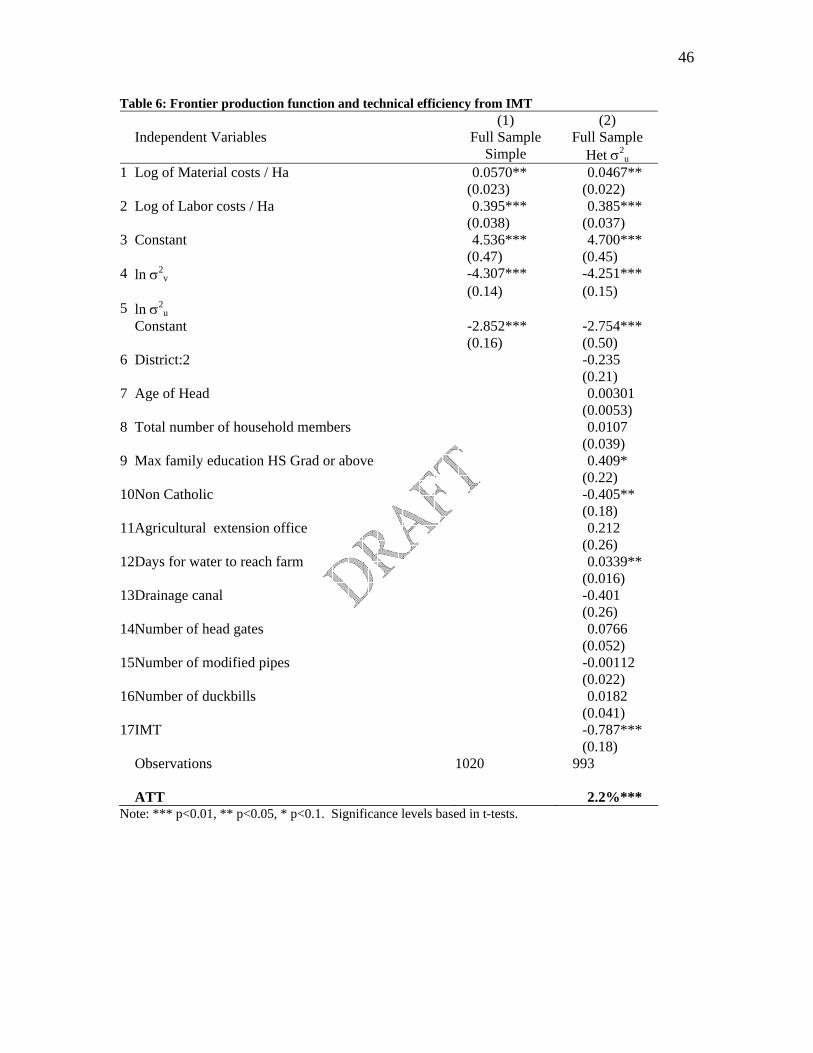
6.3. Stochastic Frontier Results

The stochastic frontier yield estimations without the heteroskedasticity of the technical

efficiency term are presented in column 1 of Table 6. The input coefficients are

statistically significant and similar in size and sign as compared with the OLS estimations

in Column 1 of Table 4. In Table 6, null hypothesis that σ 2u = 0 is rejected at better than

1 percent level of significance. This implies that the difference between the observed rice

productivity and the frontier rice productivity is not due to statistical variability alone but

also due to technical inefficiency of the households.

Column 2 adds the heteroskedasticity component to the error term associated with the

technical inefficiency error term u in the equation (4). The second part of Column 2

shows the estimates of heteroskedastic estimation of (5). The coefficient for IMT in (5)

is negative and significant at better than 1 percent level. This implies IMT reduces the

variability in the technical inefficiency. That is, households in IMT areas would have

30

lower variability in technical inefficiency. Thus, the IMT coefficient in column 2 of table

6 is not comparable to that in column 2 of table 4.

The ATT impact of IMT on rice yield is presented at the bottom row of Table 6. The

average increase in yield attributable to IMT for the households in IMT-IAs is 2.2

percent. As expected the estimates of increase in yields using stochastic frontier methods

are lower than the increase in yield estimated by the OLS results.

6.4. Rich and Poor

Table 7 shows the OLS estimators of the yield functions for the rich and poor households.

IMT has an impact on rice yield for both the rich households, Column (1), and for poor

households, Column (2). A 9 percent boost in rice yield for poor households can be

attributed to the IMT whereas the increase in rice yield for rich households is 4 percent.

The 5 percent difference in the gain in rice yield for the poor as compared with the rich is

statistically significant at 5 percent level. Thus, we find no evidence of elite capture in

IMT IAs. The poor households in IMT IAs tend to gain more from IMT as compared

with the rich households there.

Table 8 shows the stochastic frontier estimators of the yield functions for the rich and

poor households. IMT is a significant negative factor determining the heteroskedasticity

of the technical inefficiency in the estimations for both the rich and poor households. The

average yield increase attributable to IMT for rich households range between 1.7 percent

31

to 2.1 percent and that for the poor households ranges from 3.4 percent to 5.1 percent. As

expected the stochastic frontier estimates are lower than the OLS estimates. The gain in

yield attributable to IMT for the poor households is double or more as compared with the

gain for the rich households. The relative gain in yield for the poor as compared with the

rich are of similar magnitude (double or more) irrespective of the type of estimator OLS

or stochastic frontier.

In order to understand why the poor appear to gain from IMT, we examine some

additional questions asked the survey. Table 9 provides information on the how the poor

view irrigation water delivery and offers some insights into why the poor may be slightly

better off under IMT. A larger percentage of the poor (32%) in IMT IAs are downstream

farmers relative to the poor in non-IMT IAs (24%). Further, significantly more of the

poor farmers in IMT IAs (relative to poor in non-IMT IAs) indicate that the IAs help

resolve illegal use of water. Similarly, significantly more of the IMT IA poor indicate

that the water distribution schedule is followed.4 Thus, one explanation for the boost

IMT appears to give the poor lies in the fact that IMT helps increase timeliness of water

delivery in general, and, more specifically, downstream availability of water. A recent

review of IMT worldwide suggests that one of the ways management transfer can help

poor farmers is by increasing the flow of water from upstream to downstream areas

(Araral 2005). Our results appear to back this conclusion.

4T-tests show these differences between asset poor farmers in IMT IAs and non-IMT IAs are statistically

significant.

32

7. Conclusions

Irrigation Management Transfer is an important strategy among donors and governments

to strengthen farmer control over water. IMT is also a means to reduce the financial

burdens of fiscally strapped national irrigation associations. In this study, we seek to

understand if IMT is meeting the promise of its commitments. Our objective is to

understand whether IMT results in improvements in both irrigation system indicators and

in some household indicators.

We draw several important conclusions from this analysis. First, IMT contributes to an

increase in maintenance activities undertaken by irrigation associations. While

associations with and without IMT contracts both undertake canal maintenance, the

frequency of maintenance in IMT IAs is higher.

By increasing local control over water delivery, IMT also increases rice yields by 2 to

6%. Rice production in IMT IAs is higher even after we control for various differences

amongst rice farmers in IMT and non-IMT IAs. Our analysis shows that IMT contributes

to a reduction in technical inefficiencies in production.

IMT is, at a minimum, poverty-neutral, and may even give the asset-poor a boost in terms

of rice yields. We speculate that this boost may be related to increased timeliness of

water availability and improved conflict resolution related to illegal use and maintenance.

33

Quantitative impact analyses of interventions such as irrigation management transfer are

best done with pre-intervention and post-intervention data. In this study, we do not have

base-line information on irrigation and farm yields prior to IMT -- instead we compare

farmers affected by the intervention and those who are not. Further, our study is based on

farmer and irrigation association member responses rather than any physical measures of

irrigation indicators. Thus, there are various ways in which this study can be improved.

Our conclusions, however, do offer some new insights into irrigation management that

should be useful for promoting irrigation reform in the Philippines as well as fostering

decentralization in water management in other parts of the world.

34

Acknowledgements

We are grateful to the Trust Fund for Environmentally and Socially Sustainable

Development for providing financial assistance for this study. First, we would like to

acknowledge Kirk Hamilton, Team Leader Policy and Economics Team for his

encouragement and leadership. This work was undertaken in part to support on-going

analytical work on irrigation management transfer lead by Mie Xie in the East Asia Rural

Development Department of the World Bank. We are grateful to Mie and her team for

their help and feed-back. We would also like to acknowledge Project Manager Cristina

Dela Paz, and survey team leaders Antonia Carlos, and Milagros Tetangco from

Hassall/SDS and Associates and their team for doing an excellent job with the household

and irrigation association surveys, and, all the respondents who patiently answered the

survey questions.

35

References

Abadie, A., Drukker, D., Herr, H., and Imbens, G., 2003. Implementing matching

estimators for average treatment effects in STATA, Department of Economics,

University of California, Berkeley, unpublished manuscript.

Adhikari, B., 2003. Property rights and natural resources: socio-economic heterogeneity

and distributional implications of common property resource management. Working

Paper 1-03. South Asian Network for Development and Environment Economics

(SANDEE): Katmandu, Nepal.

Araral, E., 2005. Water user associations and irrigation management transfer:

understanding impacts and challenges. In: Shyamsundar, P., Araral, E., and Weerartne,

S., (Ed.) Devolution of Resource Rights, Poverty, and Natural Resource Management – A

Review. Environment Department Paper No. 104, World Bank.

Baland, J-M., and Plattaeu, J-P., 1996. Halting degradation of natural resources. Is there

a role for rural communities? Oxford, U.K: FAO and Oxford University Press.

Bagadion, B., 2002. Role of Water Users Associations for Sustainable Irrigation

Management. In: Organizational Change for Participatory Irrigation Management,

Report of the APO Seminar on Organizational Change for Participatory Irrigation

36

Management, Philippines, 23-27 October 2000. Asian Productivity Organization, Tokyo,

Japan.

Battese, G., and Coelli, T., 1995. A model for technical efficiency effect in a stochastic

frontier production function for panel data, Empirical Economics 20, 325-332.

Bardan, P., 2000. Irrigation and cooperation: An empirical analysis of 48 irrigator

communities in Southern India. Economic Development and Cultural Change, 48, 847-

865.

Barrett, C.B., Moser, C.M., McHugh, O.V., Barison, J., 2004. Better Technology, better

plots or better farmers? Identifying changes in productivity and risk among Malagasy

rice farmers, American Journal of Agricultural Economics, 86, 4, 869-888.

Birkhaeuser, D., Evenson, R.E. and Feder, G., 1991. The economic impact of agricultural

extension: A review, Economic Development and Cultural Change, 39, 3, 607-650.

Bindlish, V. and Evenson, R.E., 1997. The impact of T&V extension in Africa: The

experience of Kenya and Burkina Faso, The World Bank Research Observer, 12, 2, 183-

201.

37

Fan, S., 1991. Effects of technological change and institutional reform in production

growth in Chinese agriculture, American Journal of Agricultural Economic, 73, 2, 266-

275.

Fujuiie, M., Hayami, Y., and M. Kikuchi. 2005. The conditions of collective action for

local commons management: the case of irrigation in the Philippines, Agricultural

Economics 33, 179-189.

Hassall and Associates International (in association with Sustainable Development

Solutions). 2004. Philippines: Irrigation Management Transfer (IMT) Field Survey.

Phase 1: IMT performance survey. Final report, September, 2004.

Imbens, G.W., 2004. Nonparametric estimation of average treatment effects under

exogeneity: A review, Review of Economics and Statistics, 86, 1, 4-29

Kloezen, W., Garces-Restrepo, C., and S. Johnson. 1997. Impact assessment of IMT in

the Alto Rio Lerma Irrigation District, Mexico. Research Report 15. Colombo, Sri Lanka:

IIMI.

Klooster, D., 2000a. Community forestry and tree theft in Mexico: Resistance or

complicity in conservation? Development and Change 31, 281-305.

Klooster, D., 2000b. Institutional choice, community, and struggle: A case study of forest

co-management in Mexico, World Development 28, 1, 1-20.

38

Koppen, B., Parthasarathy, R., and Safiliou, C., 2002. Poverty dimensions of IMT in

large scale canal irrigation in Andra Pradesh and Gujarat, India. Research Report 61.

Colombo, Sri Lanka: IWMI.

Kumbhakar, S.C., and Lovell, C.A.K., 2000. Stochastic frontier analysis. Cambridge

University Press, Cambridge, 344 pp.

Meinzen-Dick, R., Raju, K.V., Gulati, A., 2002. What Affects Organization and

Collective Action for Managing Resources? Evidence from Canal Irrigation Systems in

India, World Development, 30,4, 649-666.

Mejia, A.M. 2002. Participatory irrigation management in the Philippines: Issues and

constraints. In Organizational Change for Participatory Irrigation Management, Report

of the APO Seminar on Organizational Change for Participatory Irrigation Management,

Philippines, 23-27 October 2000. Asian Productivity Organization, Tokyo, Japan.

Ostrom, E. 1990. Governing the commons: The evolution of institutions for collective

action. Cambridge University Press, Cambridge, 298 pp.

Ravallion, M., 2001. The mystery of the vanishing Benefits: An introduction to impact

evaluation, The World Bank Economic Review, 15, 1, 115-140

39

Sabio, E.A. and Mendoza, A.D., 2002. Philippines. In Organizational Change for

Participatory Irrigation Management, Report of the APO Seminar on Organizational

Change for Participatory Irrigation Management, Philippines, 23-27 October 2000.

Asian Productivity Organization, Tokyo, Japan.

Shah, T., Koppen, B., Merrey, D., Lange, M., and Samad, M., 2002. Institutional

alternatives in African small holder irrigation: Lessons from international experience with

IMT.: Research Report 60. Colombo, Sri Lanka: International Water Management

Institute.

Vermillion, D. L. 1992. Irrigation management turnover: Structural adjustment or

strategic evolution?” IIMI Review 6, 2, 3–12.

Vermillion, D. L. 1997. Impacts of Irrigation Management Transfer: A review of the

evidence. Research Report 11. Colombo, Sri Lanka: IIMI.

Wang, J. Z. Xu, J. Huang and S. Rozelle. 2006. Incentives to managers or participation

of farmers in China’s irrigation systems: which matters most for water savings, farmer

income, and poverty? Agricultural Economics 34, 315-330.

World Bank, 2001. Second Irrigation Operations Support Project (IOSP II). Republic of

the Philippines. Implementation Completion Report. Rural Development and Natural

Resources Sector Unit, East Asia and Pacific Region.

40

Figure 1: The linkages between IMT, Irrigation Association Activities and Farm Productivity

Increased revenue collection and access Increased control over water schedules

Ability to reduce conflicts Mandate to undertake maintenance

Improved timeliness of delivery in Up-stream and downstream areas

Increased certainty about water availability Increased quantity of water

Reduced inefficiency Improved yields

Changes in distribution

IA Changes

Irrigation Management Transfer

National Irrigation Association

Water Impacts

Farmer Benefits

41

Table 1: Differences between Irrigation Associations in IMT and non-IMT Areas

Mean IMT Mean

Non-IMT Mean

Difference in Mean

IA Location and Size 1 Distance from head gate (KM) 5.5 5.9 4.8 1.1 2 % IA Located Upstreem 25.0% 32.6% 12.0% 20.6% ** 3 % IA Located Midstreem 30.9% 30.2% 32.0% -1.8% 4 % IA Located Downstreem 44.1% 37.2% 56.0% -18.8% 6 Total area under IA 218 218 219 -1 7 Farmers IA members 151 165 128 37 **

IA Infrastructure 12 Length of lined canal / lateral 0.09 0.14 0.01 0.13 * 15 Number of turnouts 8.1 8.6 7.3 1.4 * 16 Number of modified pipes 1.5 2.0 0.5 1.5 **

IA Governance 18 Percent of members paying ISF 65.6% 66.7% 63.5% 3.3% 21 Number of board members 10.6 11.5 9.2 2.3 *** 22 Number of female board members 0.2 0.2 0.2 0.0 24 % IA involved by NIA in system operational plans 43.0% 42.0% 44.0% -2.0% 26 % IA operating gates 47.0% 72.0% 4.0% 68.0% ***

IA Maintenance 27 % IA solely responsible for canal maintenance 49.0% 72.0% 8.0% 64.0% *** 28 % IA where NIA and IA are jointly responsible for canal maintenance 16.0% 23.0% 4.0% 19.0% ** 29 % IA Prepare maintenance plan every year 45.6% 62.8% 16.0% 46.8% *** 30 % IA Canal cleaning more than twice a season or when needed 47.1% 62.8% 20.0% 42.8% *** 31 % IA where paid participation is most common 23.5% 32.6% 8.0% 24.6% ***

Note: *** p<0.01, ** p<0.05, * p<0.1. Significance levels based on t-tests.

42

Table 2: Differences between Households in IMT IAs and non-IMT IAs

Combined NON-IMT Differen

ce Mean

IMT Mean Mean in Mean

Household Characteristics (% of households) 1 Walling materials of house made of concrete blocks 85.00% 85.60% 84.00% 1.60% 2 Max HH education of HS graduate 19.90% 20.30% 19.20% 1.10% 3 Max HH Education of College graduate 38.90% 38.60% 39.50% -0.90% 4 Average age of household (years) 34 34 34 0

Agricultural Output and Input 5 Output / Ha (Peso) 41823 42512 40638 1875 *** 6 Output (Kg) / Ha 5230 5366 4996 369 *** 7 Material costs (peso) / Ha 9017 9764 7732 2032 8 Labor costs (peso) / Ha 11859 11984 11644 340 9 Area harvested - Palay dry season (Ha) 2.4 2.4 2.3 0

10 Area harvested - Palay wet season (Ha) 2.4 2.4 2.3 0 Livestock, Assets and Protein Food Consumption

11 Value of Livestock (Peso) 27383 26343 29172 -2829 12 Value of Assets (Peso) 75778 80381 67862 12519 * 13 Protein Food Cons. Expd (Peso) 830 795 890 -95

Irrigation (% yes) 14 Water distribution schedule followed 71.60% 74.90% 65.90% 9.00% *** 15 Illegal checking sometimes 31.70% 30.40% 33.90% -3.50% 16 Never any unscheduled gate opening/closing 56.10% 57.70% 53.30% 4.30% * 17 IA helps resolve illegal checking 85.00% 87.70% 80.50% 7.20% *** 18 IA helps resolve illegal pumping 84.10% 89.20% 75.30% 13.80% *** 19 IA helps resolve illegal turnout 83.50% 86.90% 78.00% 9.00% *** 20 IA helps resolve unscheduled gate opening/closing 85.80% 88.50% 81.50% 7.00% ***

21 Household often participates in maintenance of main farm ditch 73.00% 75.30% 69.10% 6.30% **

22 Household often participates in maintenance of sub-laterals 62.00% 64.50% 57.60% 6.90% **

23 Household often participates in maintenance of laterals 62.40% 65.10% 57.60% 7.50% *** Perception of Change in the last five years (% yes)

24 Improvement in cropping intensity 5.30% 4.80% 6.10% -1.30% 26 Improvement in IA services 33.10% 36.60% 27.20% 9.40% *** 27 Improvement in farmer participation in O&M 44.00% 47.00% 38.90% 8.00% *** 28 Improvement in water delivery timeliness 32.10% 34.60% 27.70% 6.80% **

Note: *** p<0.01, ** p<0.05, * p<0.1. Significance levels based on t-tests.

43

Table 3: Propensity Score and Instrumental Variable Estimations of the Impact of IMT on Irrigation Association Performance

Note: *** p<0.01, ** p<0.05, * p<0.1. Significance levels based on t-tests.

Propensity Score Measures of IMT Effect on Outcome

Effect of IMT on

Outcome

(1) (2) (3) (4) (5)

Outcome Kernel Radius Nearest

Neighbor Stratifi- cation

Instrument Variable

Maintenance

1 Prepare maintenance plan every year 15.4% 23.6% 30.2% -27.0% 47.8% **

2

Canal reshaping more than twice a season or when needed 61.5% *** 80.9% *** 62.8% *** 63.7% *** 60.6% ***

ISF Collection

4 Collection Efficiency in 2003 dry season 16.9% ** 36.8% 19.0% ** 20.6% 10.4%

44

Table 4: IMT Effect on Rice Production (1) (2) (2) OLS OLS with Shift

Variables Instrumental

Variable 1 Log of Material costs / Ha 0.072*** 0.072** 0.071** (0.027) (0.032) (0.031) 2 Log of Labor costs / Ha 0.434*** 0.440*** 0.441*** (0.041) (0.045) (0.045) 3 District:2 0.039** 0.040** (0.018) (0.018) 4 Age of Head -0.001 -0.001 (0.000) (0.000) 5 Total number of household members 0.001 0.001 (0.003) (0.003) 6 Max family education HS Grad or

above -0.032** -0.033**

(0.014) (0.014) 7 Non Catholic 0.036** 0.037*** (0.014) (0.014) 8 Agri extension office -0.038 -0.037 (0.023) (0.023) 9 Days for water to reach farm -0.003* -0.003** (0.001) (0.001) 10 Drainage canal 0.044* 0.044** (0.023) (0.023) 11 Number of head gate -0.011*** -0.011*** (0.003) (0.003) 12 Number of modified pipes 0.000 0.000 (0.003) (0.003) 13 Number of duckbill 0.002 0.003 (0.005) (0.005) 14 IMT 0.058*** 0.053*** (0.016) (0.018) 15 Constant 3.847*** 3.754*** 3.757*** (0.53) (0.650) (0.646) Observations 1020 993 993 R-squared 0.31 0.36 Note: *** p<0.01, ** p<0.05, * p<0.1. Significance levels based on t-tests. @ Table 5 presents the second regression used in the instrumental variable approach.

45

Table 5: Probit regression of IMT on Independent Variables Coefficents (SE) 1 District:2 -2.484*** (0.875) 2 Median edu of head is >= HS Grad 0.912 (0.814) 3 % sample HH Catholic in IA -5.249*** (1.755) 4 Avg Yrs HH member of Other User Groups 0.641*** (0.171) 5 Avg Land size (ha) per HH in IA 0.853** (0.365) 6 Land Gini by IA 2.185 (1.842) 7 Farmers IA members 0.017*** (0.005) 8 Length of canal / lateral -0.493 (0.450) 9 Number of head gate -0.566* (0.332) 10 Number of modified pipes 0.974*** (0.251) 11 Number of duckbill 0.378** (0.159) 12 IA with post office 0.395 (0.609) 13 Ratio of IMT-IA in Municipality 12.696*** (2.628) 14 Constant -9.368*** (2.965) ρ 0.065 (0.055) Log σ -1.700*** (0.057) Observations 993 Note: *** p<0.01, ** p<0.05, * p<0.1. Significance levels based in t-tests.

46

Table 6: Frontier production function and technical efficiency from IMT (1) (2)

Independent Variables

Full Sample Simple

Full Sample Het σ2

u 1 Log of Material costs / Ha 0.0570** 0.0467** (0.023) (0.022) 2 Log of Labor costs / Ha 0.395*** 0.385*** (0.038) (0.037) 3 Constant 4.536*** 4.700*** (0.47) (0.45) 4 ln σ2

v -4.307*** -4.251*** (0.14) (0.15) 5 ln σ2

u Constant -2.852*** -2.754*** (0.16) (0.50) 6 District:2 -0.235 (0.21) 7 Age of Head 0.00301 (0.0053) 8 Total number of household members 0.0107 (0.039) 9 Max family education HS Grad or above 0.409* (0.22) 10 Non Catholic -0.405** (0.18) 11 Agricultural extension office 0.212 (0.26) 12 Days for water to reach farm 0.0339** (0.016) 13 Drainage canal -0.401 (0.26) 14 Number of head gates 0.0766 (0.052) 15 Number of modified pipes -0.00112 (0.022) 16 Number of duckbills 0.0182 (0.041) 17 IMT -0.787*** (0.18) Observations 1020 993 ATT 2.2%*** Note: *** p<0.01, ** p<0.05, * p<0.1. Significance levels based in t-tests.

47

Table 7: IMT Effect on Rice Production – Poor and Rich Differences (1) (2) Sl. N. Independent Variables Asset Rich Asset Poor 1 Log of Material costs / Ha 0.050 0.095** (0.037) (0.047) 2 Log of Labor costs / Ha 0.378*** 0.551*** (0.048) (0.085) 3 District:2 0.044*** 0.036 (0.016) (0.030) 4 Age of Head -0.000 -0.001 (0.000) (0.001) 5 Total number of household members 0.001 -0.001 (0.005) (0.005) 6 Max family education HS Grad or above -0.025 -0.041* (0.026) (0.024) 7 Non Catholic 0.034** 0.045 (0.014) (0.027) 8 Agri extension office -0.034 -0.049 (0.034) (0.033) 9 Days for water to reach farm -0.002 -0.003 (0.002) (0.003) 10 Drainage canal 0.030 0.059** (0.028) (0.027) 11 Number of head gate -0.010** -0.011** (0.004) (0.005) 12 Number of modified pipes 0.002 -0.003 (0.002) (0.004) 13 Number of duckbill -0.001 0.006 (0.005) (0.006) 14 IMT 0.036** 0.089*** (0.016) (0.026) 15 Constant 4.548*** 2.503** (0.684) (1.130) Observations 592 401 R-squared 0.32 0.42

Note: *** p<0.01, ** p<0.05, * p<0.1. Significance levels based in t-tests.

48

Table 8: Frontier production function for asset rich and asset poor

(1) (2) Independent Variables

Asset Rich Asset Poor

Log of Material costs / Ha 0.0337 0.0607** (0.034) (0.025) Log of Labor costs / Ha 0.353*** 0.441*** (0.050) (0.049) Constant 5.120*** 4.024*** (0.66) (0.54) ln σ2

v -4.268*** -4.066*** (0.18) (0.38) ln σ2

u Constant -2.829*** -3.369** (0.67) (1.52) District:2 -0.565** 0.236 (0.26) (0.38) Age of Head -0.00186 0.0112 (0.0074) (0.012) Total number of household members 0.0318 0.00688 (0.052) (0.072) Max family education HS Grad or above 0.280 0.574 (0.31) (0.62) Non Catholic -0.479** -0.436 (0.23) (0.38) Agricultural extension office 0.454 -0.0377 (0.39) (0.37) Days for water to reach farm 0.0263 0.0530* (0.018) (0.031) Drainage canal -0.143 -0.478 (0.27) (0.43) Number of head gates 0.116 0.00169 (0.079) (0.089) Number of modified pipes -0.0529* 0.0417 (0.031) (0.046) Number of duckbills 0.0201 0.0225 (0.053) (0.071) IMT -0.596*** -1.132** (0.23) (0.52) Observations 592 401 ATT 1.7%*** 3.4%*** Note: *** p<0.01, ** p<0.05, * p<0.1. Significance levels based in t-tests.

49

Table 9: Differences in perceptions about irrigation water delivery among asset poor in IMT and non-IMT areas Questions Regarding Timeliness of Water

Delivery and Conflict Resolution Percent of Asset Poor who said Yes

Total IMT IA NON-IMT IA

Difference

1 Is the water distribution schedule followed? 71.1% 75.3% 63.8% 11.5%*** 2 Does the IA help resolve illegal checking? 84.2% 88.7% 77.1% 11.7%*** 3 Does the IA help resolve illegal pumping? 84.9% 92.2% 73.4% 18.7%*** 4 Does the IA help resolve illegal turnout? 84.4% 89.7% 76.3% 13.3%*** 5 Does the IA help resolve unscheduled gate

opening/closing? 87.1% 90.9% 81.9% 9.0%**

6 Is your farm located downstream? 29.4% 32.4% 24.2% 8.3%** 7 Do you get water when needed during the dry

season? 65.4% 70.9% 55.7% 15.2%***

8 Do you get water when needed during the wet season?

95.6% 96.1% 94.6% 1.5%

9 Did you pay your irrigation service fees twice in the last two seasons?

90.7% 92.7% 87.2% 5.4%**

Note: *** p<0.01, ** p<0.05, * p<0.1. Significance levels based in t-tests.

50

Table 1A: Instrument Variable coefficients of Impact Evaluation (1) (2) (3) (4) (5) (6) COEFFICIENT Prepare

maintenance plan every year

IMT Canal Reshaping >2 a season or when

need

IMT Collection Efficiency 03

Dry

IMT

District:2 0.157 -2.490*** 0.166 -2.490*** -0.0454 -2.490** (0.12) (0.83) (0.13) (0.90) (0.076) (0.98) Median edu of head is >= HS Grad

0.0170 0.903 0.0670 0.903 -0.220 0.903

(0.12) (0.80) (0.12) (0.82) (0.16) (1.22) Percent Catholic

0.0256 -5.301*** 0.441* -5.301*** 0.123 -5.301

(0.28) (1.87) (0.25) (1.70) (0.39) (3.23) Avg Yrs HH member of Other User

0.00370 0.643*** -0.0643** 0.643*** -0.0172 0.643**

(0.033) (0.17) (0.031) (0.17) (0.022) (0.32) Avg Land size (ha) per HH in IA

-0.0912* 0.851** -0.0553 0.851** 0.0460 0.851***

(0.050) (0.37) (0.053) (0.39) (0.034) (0.31) Land Gini by IA

-0.400 2.135 -0.764* 2.135 -0.569 2.135

(0.53) (2.08) (0.43) (1.71) (0.59) (2.73) Farmers IA members

0.0000746 0.0168*** -0.00149*** 0.0168*** -0.000389 0.0168***

(0.00072) (0.0057) (0.00056) (0.0055) (0.00064) (0.0053) Length of canal / lateral

0.120** -0.472 -0.0435 -0.472 0.0881*** -0.472

(0.054) (0.47) (0.051) (0.46) (0.030) (0.50) Number of head gate

0.0428 -0.565 -0.0334 -0.565 -0.0152 -0.565

(0.040) (0.40) (0.044) (0.38) (0.024) (0.38) Number of modified pipes

0.00776 0.976*** -0.00276 0.976*** 0.0120 0.976***

(0.017) (0.26) (0.014) (0.23) (0.0087) (0.20) Number of duckbill

0.0264 0.385** 0.0333 0.385** 0.00246 0.385**

(0.030) (0.17) (0.026) (0.16) (0.022) (0.16) IA with post office

-0.0786 0.420 -0.0954 0.420 -0.0749 0.420

(0.13) (0.60) (0.10) (0.62) (0.12) (1.12) IA with IMT Contract

0.478** 0.606*** 0.104

(0.20) (0.15) (0.35) Ratio of IMT-IA in Municipality

12.77*** 12.77*** 12.77

(2.73) (2.55) (0) Constant -0.0315 -9.454*** 0.891*** -9.454*** 0.681*** -9.454*** (0.33) (3.04) (0.26) (3.12) (0.24) (2.33) Observations 67 67 67 67 66 66

Robust standard errors in parentheses *** p<0.01, ** p<0.05, * p<0.1