dr ian r. manchester - university of...
TRANSCRIPT
Dr Ian R. Manchester
Dr Ian R. Manchester AMME 3500 : Review
Slide 2 Dr Ian R. Manchester Amme 3500 : Review
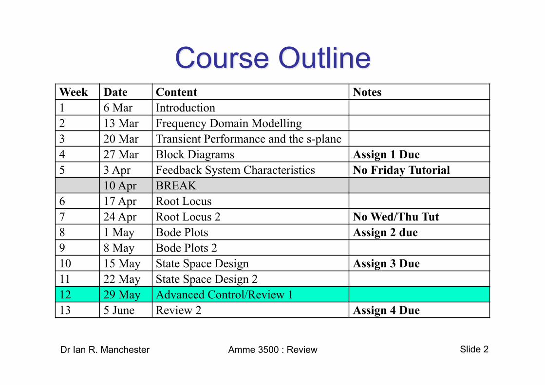
Week Date Content Notes 1 6 Mar Introduction 2 13 Mar Frequency Domain Modelling 3 20 Mar Transient Performance and the s-plane 4 27 Mar Block Diagrams Assign 1 Due 5 3 Apr Feedback System Characteristics No Friday Tutorial
10 Apr BREAK 6 17 Apr Root Locus 7 24 Apr Root Locus 2 No Wed/Thu Tut 8 1 May Bode Plots Assign 2 due 9 8 May Bode Plots 2 10 15 May State Space Design Assign 3 Due 11 22 May State Space Design 2 12 29 May Advanced Control/Review 1 13 5 June Review 2 Assign 4 Due

Slide 3 Dr Ian R. Manchester AMME 3500 : Review
• 4 Assignments (40%) – Assignment 1 : Due Week 4 (5%) – Assignment 2 : Due Week 6 (10%) – Assignment 3 : Due Week 10 (10%) – Assignment 4 : Due Week 13 (15%)
• Final Exam (60%)*
* Note you are expected to pass the exam to pass this course
Slide 4 Dr Ian R. Manchester AMME 3500 : Review
• To introduce the methods used for the analysis and design of feedback controllers for linear time invariant (LTI) systems

Slide 5 Dr Ian R. Manchester AMME 3500 : Review
• System 1 affects system 2, which affects system 1, which affects system 2….
System 1 (e.g. Controller)
System 2 (e.g. Process)

Slide 6 Dr Ian R. Manchester AMME 3500 : Review
– Vehicle Control and Design (land, sea, air, space) – understanding and controlling how the system responds to external disturbances
– Biomedical (cardiac system, dialysis machine) – design and control of systems that interact with the human body.
– Manufacturing Processes – controlled conditions for high-performance materials, pharmaceuticals, microsystems.
– Biological – feedback systems that regulate pressures, concentrations, balance, etc
Slide 7
• Design the dynamics – Sluggish systems become quick to respond – Unstable systems become stable and predictable
• “Robustness” – Reject disturbances acting on the system – Same response with large variations in the system
Dr Ian R. Manchester AMME 3500 : Review

Slide 8
• Instability: any feedback loop allows for the possibility of instability. The question of stability has long been central in control theory
• Measurement noise gets feed back into the actual system response.
Dr Ian R. Manchester AMME 3500 : Review
Slide 9 Dr Ian R. Manchester AMME 3500 : Review
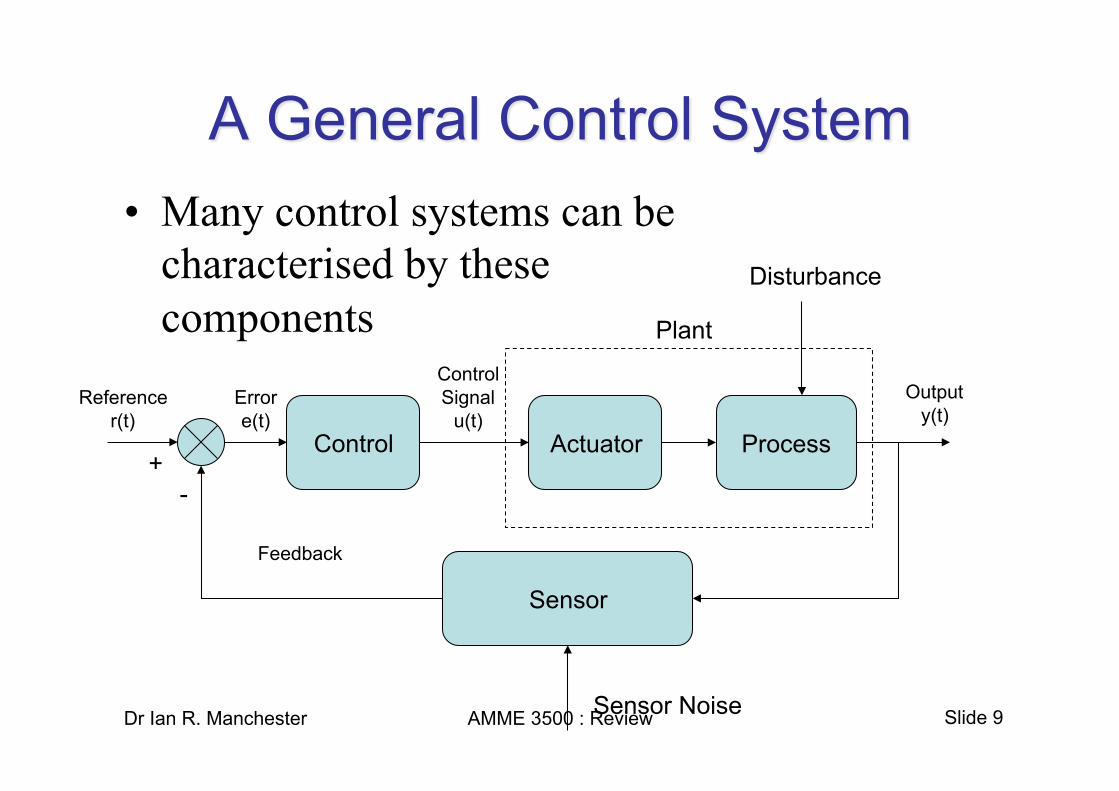
• Many control systems can be characterised by these components
Sensor
Actuator Process Control
Reference r(t)
Output y(t)
- +
Error e(t)
Control Signal
u(t)
Plant
Disturbance
Sensor Noise
Feedback

Slide 10 Dr Ian R. Manchester AMME 3500 : Review
• A block diagram is made up of signals, systems, summing junctions and pickoff points

Slide 11 Dr Ian R. Manchester AMME 3500 : Review
• A system model is one or more equations that describe the relationship between the system variables – often the input(s) and output(s) of the system
• For physical systems, these equations are derived from study of the physical properties of the system such as mechanics, fluids, electrical, thermodynamics, etc.

Slide 12 Dr Ian R. Manchester AMME 3500 : Review
• Force-velocity, force-displacement, and impedance translational relationships for springs, viscous dampers, and mass

Slide 13 Dr Ian R. Manchester AMME 3500 : Review
• Torque-angular velocity, torque-angular displacement, and impedance rotational relationships for springs, viscous dampers, and inertia
Slide 14 Dr Ian R. Manchester AMME 3500 : Review
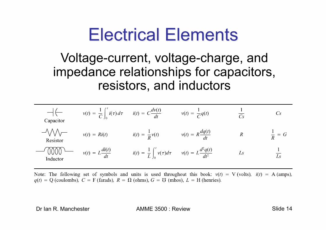
Voltage-current, voltage-charge, and impedance relationships for capacitors,
resistors, and inductors

Slide 15 Dr Ian R. Manchester AMME 3500 : Review
• Starting with an impulse response, h(t), and an input, u(t), find y(t)
u(t), h(t)
U(s), H(s)
convolution y(t)
L L-1
Multiplication, algebraic manipulation
Y(s)

Slide 16 Dr Ian R. Manchester AMME 3500 : Review
• We normally use tables of Laplace transforms rather than solving the Laplace equations directly
• This greatly simplifies the transformation process

Slide 17 Dr Ian R. Manchester AMME 3500 : Review
• The Laplace Transform is a linear transformation between functions in the t domain and s domain
Slide 18 Dr Ian R. Manchester AMME 3500 : Review
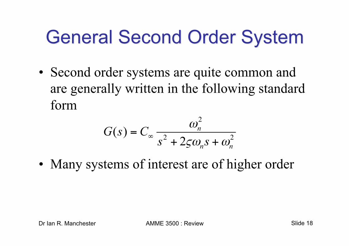
• Second order systems are quite common and are generally written in the following standard form
• Many systems of interest are of higher order
Slide 19 Dr Ian R. Manchester AMME 3500 : Review
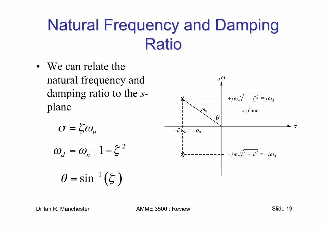
• We can relate the natural frequency and damping ratio to the s-plane
θ

Slide 20 Dr Ian R. Manchester AMME 3500 : Review
• Damping ratio determines the characteristics of the system response

Slide 21 Dr Ian R. Manchester AMME 3500 : Review
• Rise time, settling time and peak time yield information about the speed of response of the transient response
• This can help a designer determine if the speed and nature of the response is appropriate

Slide 22 Dr Ian R. Manchester AMME 3500 : Review
• For a second order system with no finite zeros, the transient response parameters are approximated by – Rise time :
– Overshoot :
– Settling Time (2%) :
Slide 23 Dr Ian R. Manchester AMME 3500 : Review
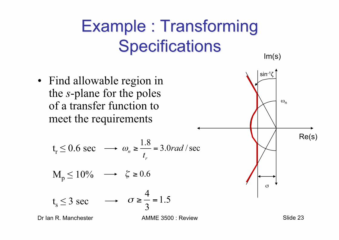
• Find allowable region in the s-plane for the poles of a transfer function to meet the requirements
tr ≤ 0.6 sec
Mp ≤ 10%
ts ≤ 3 sec
sin-1ζ
σ
ωn
Im(s)
Re(s)
Slide 24 Dr Ian R. Manchester AMME 3500 : Review
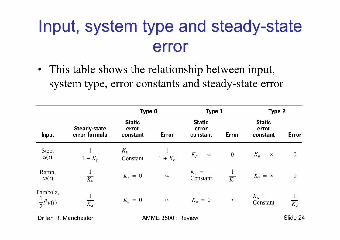
• This table shows the relationship between input, system type, error constants and steady-state error
Slide 25 Dr Ian R. Manchester AMME 3500 : Review
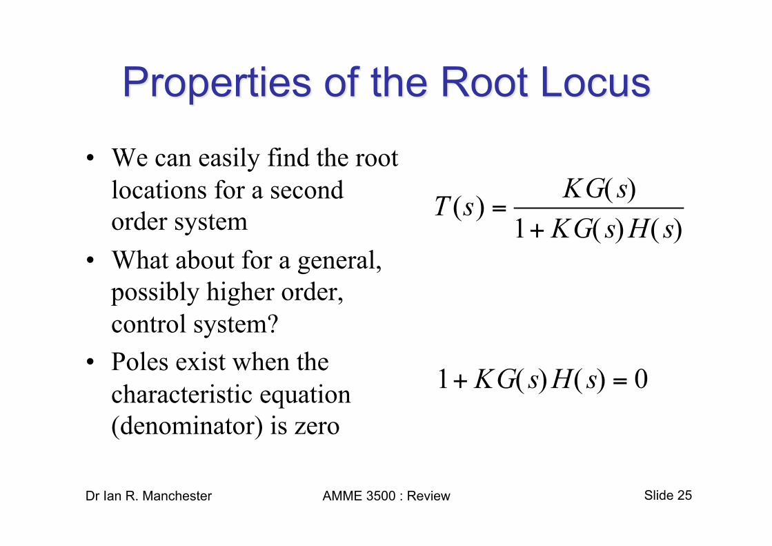
• We can easily find the root locations for a second order system
• What about for a general, possibly higher order, control system?
• Poles exist when the characteristic equation (denominator) is zero

Slide 26 Dr Ian R. Manchester AMME 3500 : Review
• The location of the roots, and hence the nature of the system performance, are a function of the system gain K
• In order to solve for this system performance, we must factor the denominator for specific values of K
• We define the root locus as the path of the closed-loop poles as the system parameter varies from 0 to ∞

Slide 27 Dr Ian R. Manchester AMME 3500 : Review
• The CL roots move from the OL towards the zeros
• Additional poles move towards infinity along well defined asymptotes
Slide 28 Dr Ian R. Manchester AMME 3500 : Review
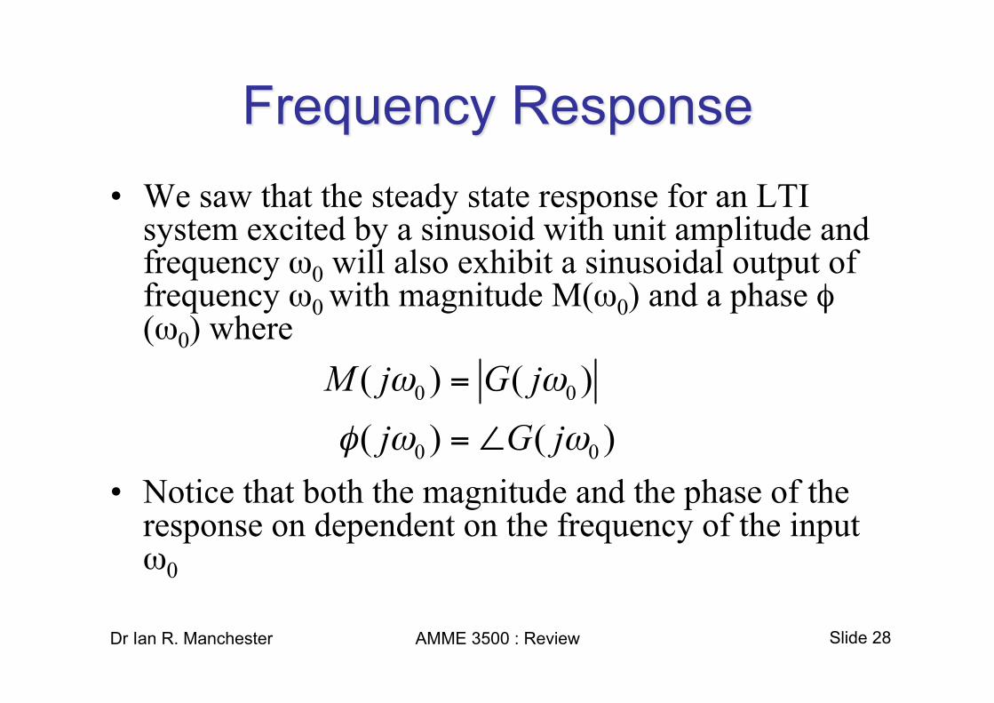
• We saw that the steady state response for an LTI system excited by a sinusoid with unit amplitude and frequency ω0 will also exhibit a sinusoidal output of frequency ω0 with magnitude M(ω0) and a phase φ(ω0) where
• Notice that both the magnitude and the phase of the response on dependent on the frequency of the input ω0

Slide 29 Dr Ian R. Manchester AMME 3500 : Review
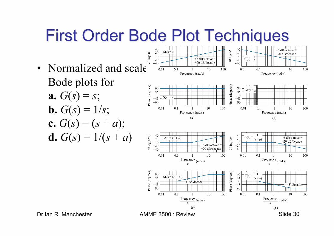
• We often plot the magnitude and phase of the system response as a function of the input frequency
• The magnitude is normally plotted in dB=20logM(ω) vs. log(ω)
• The phase is plotted in degrees vs. log(ω) • The resulting graph is called the Bode plot
Slide 30 Dr Ian R. Manchester AMME 3500 : Review
• Normalized and scaled Bode plots for a. G(s) = s; b. G(s) = 1/s; c. G(s) = (s + a); d. G(s) = 1/(s + a)
Slide 31 Dr Ian R. Manchester AMME 3500 : Review
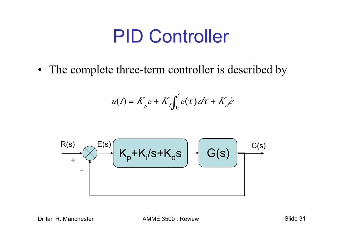
• The complete three-term controller is described by
Kp+Ki/s+Kds -
+
R(s) E(s) C(s) G(s)
Slide 32 Dr Ian R. Manchester AMME 3500 : Review
• The ideal derivative compensator effectively adds a pure differentiator to the forward path of the control system
• This is effectively equivalent to an additional zero
• As you should by now be aware, the location of the open loop poles and zeros affects the root locus and hence the transient response of the closed loop system

Slide 33 Dr Ian R. Manchester AMME 3500 : Review
• Consider a simple second order system whose root locus looks like this (roots -1, -2)
• Adding a zero to this system drastically changes the shape of the root locus
• The position of the zero will also change the shape and hence the nature of the transient response
Zero at -3
Zero at -5

Slide 34 Dr Ian R. Manchester AMME 3500 : Review
• The Bode plot for a PD controller looks like this
• The stabilizing effect is seen by the increase in phase at frequencies above the break frequency
• However, the magnitude grows with increasing frequency and will tend to amplify high frequency noise

Slide 35 Dr Ian R. Manchester AMME 3500 : Review
• For compensation using passive components, a pole and zero will result
• If the pole position is selected such that it is to the left of the zero, the resulting compensator will behave like an ideal derivative compensator
• The name Lead Compensation reflects the fact that this compensator imparts a phase lead
Slide 36 Dr Ian R. Manchester AMME 3500 : Review
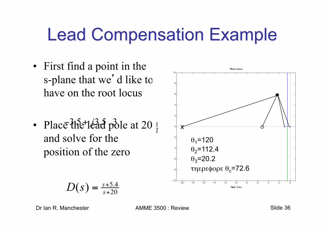
• First find a point in the s-plane that we’d like to have on the root locus
• Place the lead pole at 20 and solve for the position of the zero
x
θ1=120 θ2=112.4 θ3=20.2 τηερεφορε θc=72.6

Slide 37 Dr Ian R. Manchester AMME 3500 : Review
• The Bode plot for a Lead compensator looks like this
• The frequency of the phase increase can be designed to meet a particular phase margin requirement
• The high frequency magnitude is now limited

Slide 38 Dr Ian R. Manchester AMME 3500 : Review
• If we rewrite the transfer function for the integral compensator we find
• This is simply a pole at the origin and a zero at some other position to be selected based on our design requirements – normally close to the origin to minimize the angular contribution of the compensator
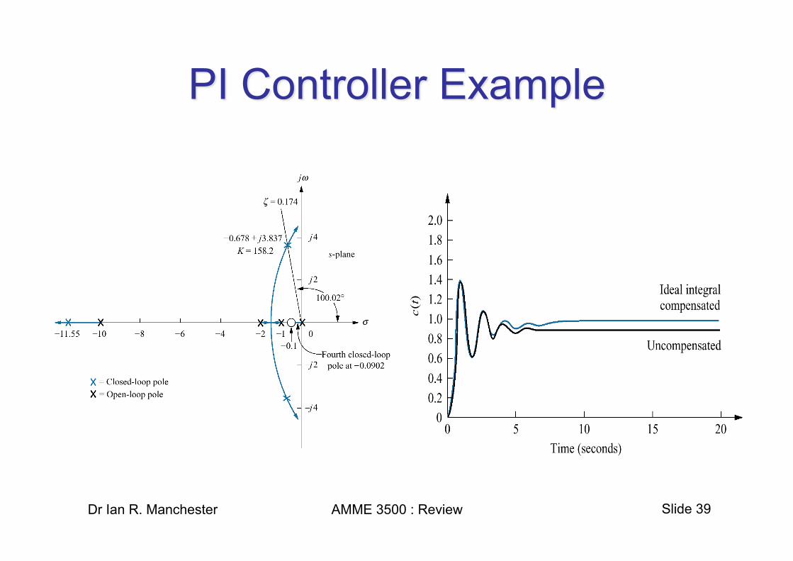
Slide 39 Dr Ian R. Manchester AMME 3500 : Review

Slide 40 Dr Ian R. Manchester AMME 3500 : Review
• The Bode plot for a PI controller looks like this
• The break frequency is usually located at a frequency substantially lower than the crossover frequency to minimize the effect on the phase margin

Slide 41 Dr Ian R. Manchester AMME 3500 : Review
• As with the lead compensation, using passive components results in a pole and zero
• If the pole position is selected such that it is to the right of the zero near the origin, the resulting compensator will behave like an ideal integral compensator although it will not increase the system type
• The name Lag Compensation reflects the fact that this compensator imparts a phase lag

Slide 42 Dr Ian R. Manchester AMME 3500 : Review

Slide 43 Dr Ian R. Manchester AMME 3500 : Review
• The Bode plot for a Lag compensator looks like this
• This compensator effectively raises the magnitude for low frequencies
• The effect of the phase lag can be minimized by careful selection of the centre frequency

Slide 44 Dr Ian R. Manchester AMME 3500 : Review
• System equations are described in matrix form. • Most fundamental are the state variables: A set of parameters
that completely describes the current state of the system. – For example position and velocity of a moving body
• Using measurements of the outputs, the system state can be computed - observers
• Using the system state, control strategies can be devised to achieve desired performance. – Pole placement – Optimal controllers
• Attractive for multi-input multi-output (MIMO) systems

Slide 45 Dr Ian R. Manchester AMME 3500 : Review
• Using the state space approach, we represent a system by a set of n first-order differential equations:
• The output of the system is expressed as:
x - state vector y - output vector u - input vector
A - state matrix B - input matrix C - output matrix D - feedthrough or feedforward matrix (often zero)

Slide 46
• We can draw a block diagram describing the general State Space Model
Dr Ian R. Manchester AMME 3500 : Review

Slide 47 Dr Ian R. Manchester AMME 3500 : Review
• We can represent a general state space system as a Block Diagram.
• If we feedback the state variables, we end up with n controllable parameters.
• State feedback with the control input
u=-Kx +r.
* N.S. Nise (2004) “Control Systems Engineering” Wiley & Sons
Slide 48 Dr Ian R. Manchester AMME 3500 : Review
• We can then control the pole locations by finding appropriate values for K
• This allows us to select the position of all the closed loop system roots during our design.
• There are a number of methods for selecting and designing controllers in state space, including pole placement and optimal control methods via the Linear Quadratic Regulator algorithm.

Slide 49
• Setting u=-Kx+r yields
• Rearranging the state equation and taking LT yields
• Select values of K so that the eigenvalues (root locations) of (A-BK) are at a particular location
Dr Ian R. Manchester AMME 3500 : Review

Slide 50
• Controllability and Observability are fundamental concepts.
• For output feedback controllers, the “separation principle” tells us that we can design an observer and a controller separately and the combined controller is stabilizing.
Dr Ian R. Manchester AMME 3500 : Review
Slide 51 Dr Ian R. Manchester AMME 3500 : Review
• You should be familiar with the concepts reviewed in this lecture – Modelling of dynamic systems – Specification of second order systems – Root Locus – Bode Plots – Design and properties of PID (and variants), Lead
and Lag controllers – State Space Modelling and Design

Slide 52 Dr Ian R. Manchester AMME 3500 : Review
• You will not be required to find roots of polynomials higher than second order.
• You will be provided with a selected set of equations you may require for solving the problems
• In order to prepare I would suggest that you – Review the assignment questions, making sure you
understand the material covered this semester – Look over previous years’ exams

Slide 53 Dr Ian R. Manchester AMME 3500 : Review
• In order to understand system performance, we must be able to model these systems
• The study of control provides us with a process for analysing, understanding and deisgning for the behaviour of a system