amme$3500/5501$:$$ system$dynamics$&$control$...

AMME 3500/5501 : System Dynamics & Control

Review 2

Dr Ian R. Manchester

Dr Ian R. Manchester AMME 3500 : Review

Dr Ian R. Manchester Amme 3500 : Review

Course Outline Week Date Content Notes 1 6 Mar Introduction 2 13 Mar Frequency Domain Modelling 3 20 Mar Transient Performance and the s-plane 4 27 Mar Block Diagrams Assign 1 Due 5 3 Apr Feedback System Characteristics No Friday Tutorial

10 Apr BREAK 6 17 Apr Root Locus 7 24 Apr Root Locus 2 No Wed/Thu Tut 8 1 May Bode Plots Assign 2 due 9 8 May Bode Plots 2 10 15 May State Space Design Assign 3 Due 11 22 May State Space Design 2 12 29 May Advanced Control/Review 1 13 5 June Review 2 Assign 4 Due

Design ObjecGves

•  The closed-‐loop system should be:

– Stable – Quick to respond, without too much overshoot – Accurate in steady state (step or ramp or …) – Able to reject disturbances and measurement errors

– Robust to model uncertainty

Benefits of Different Methods

Stable Quick,

Small OS Steady State

Reject Disturb.

Robust

Root Locus

Poles LHP Pole

locaGons #

integrators ? (poles) ?

Bode Plots

(Nyquist) (Bandwidth

phase margin)

Gain at zero freq

SensiGvity funcGons

Gain & phase margins

State Space

Eigenv. LHP

Eigenv. locaGons

Can add new states

Advanced Advanced

Dr Ian R. Manchester Amme 3500 : Bode Plots

Frequency and Stability

•  As we saw when considering the Root Locus, all points on the locus meet the following conditions

•  Substituting jω for s yields

•  A marginally stable system will satisfy these conditions



•  We can use the following condition to determine if a system is stable for a particular value of K


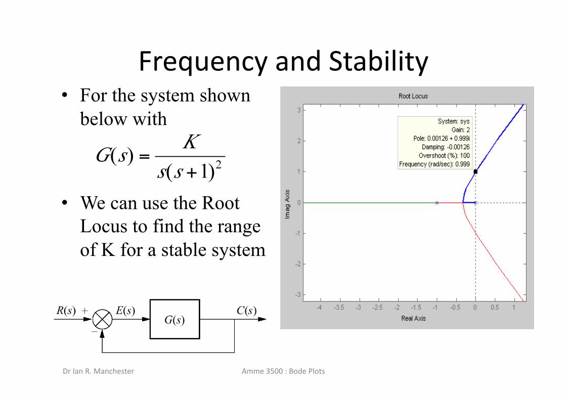
Frequency and Stability •  For the system shown

below with

•  We can use the Root Locus to find the range of K for a stable system


Gain Margin

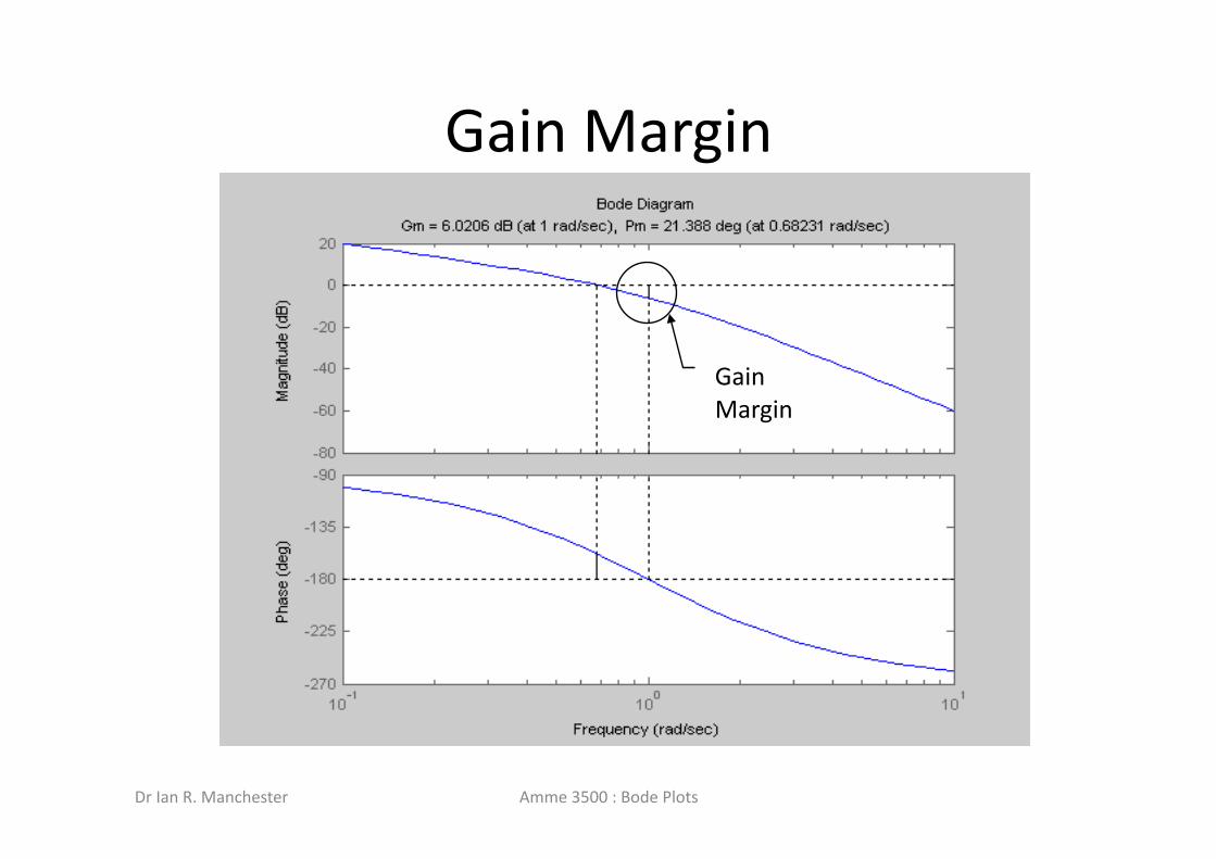
•  As we saw, the magnitude plot will rise or lower based on the system gain K

•  The gain margin is the factor by which the gain can be raised before instability results

•  This is usually read directly from the Bode plot


Gain Margin

Gain Margin


Gain Margin

•  From the plot we can see that the Gain Margin is 6.026 dB

•  This corresponds to a value of K of

•  This matches the value of K found from the Root Locus


Phase Margin

•  The stability can also be determined using the phase margin

•  This represents the amount by which the phase of G(jω) exceeds -180o when |KG(jω)|=1


Phase Margin

Phase Margin


Phase Margin

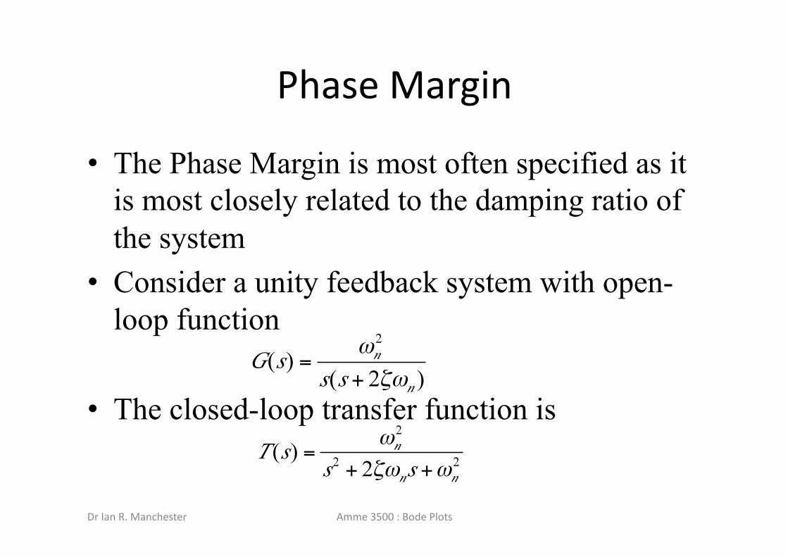
•  The Phase Margin is most often specified as it is most closely related to the damping ratio of the system

•  Consider a unity feedback system with open-loop function

•  The closed-loop transfer function is


Phase Margin

•  Recall that the phase margin occurs at the frequency for which |G(jω)|=1

•  After some manipulation, we find


Bandwidth

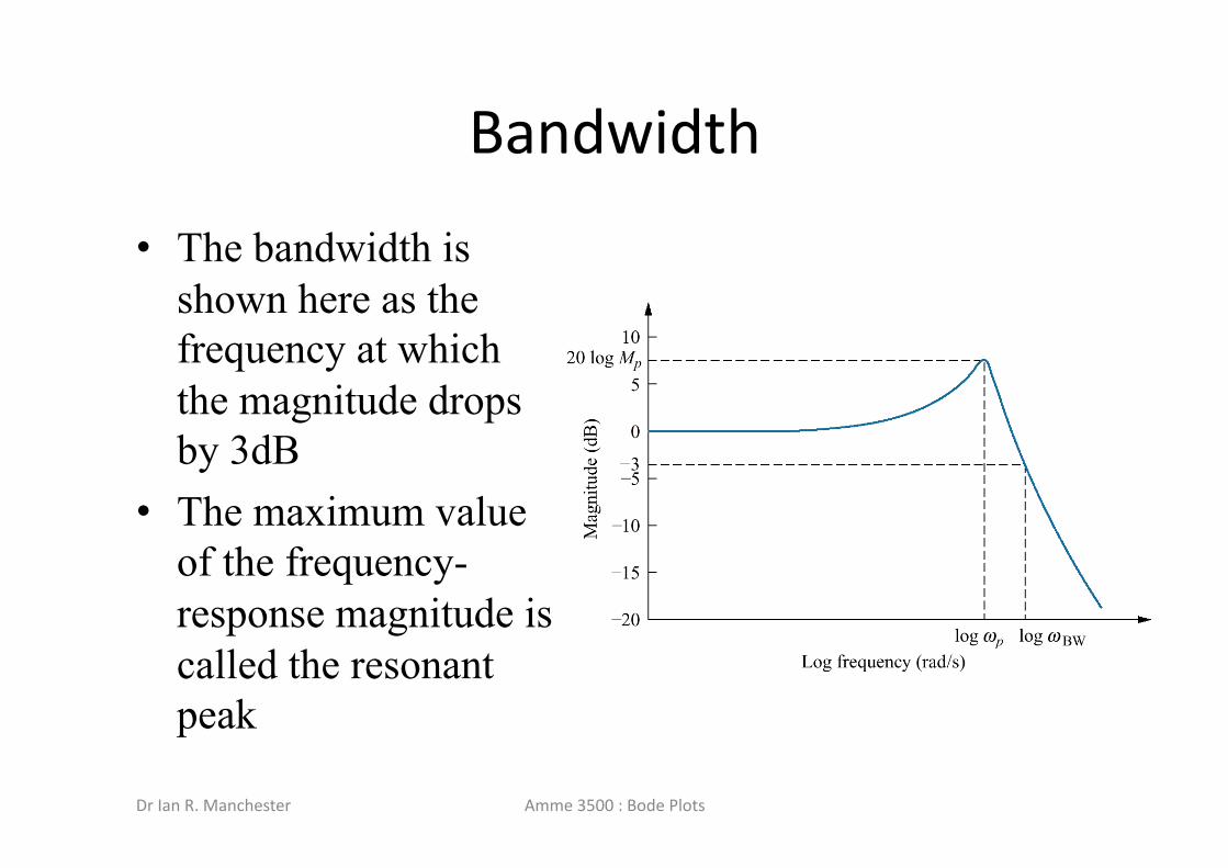
•  A common specification for system performance in terms of frequency response is the bandwidth

•  This is defined to be the maximum frequency at which the output of a system will track an input sinusoid with attenuation of less than 3dB


Bandwidth

•  The bandwidth is shown here as the frequency at which the magnitude drops by 3dB

•  The maximum value of the frequency-response magnitude is called the resonant peak


Bandwidth and Time Response

•  To relate ωBW to settling time, substitute

•  Yielding

•  And since

•  Peak time can be found as


•  The bandwidth of the closed-loop system is related to the speed of response

Open Loop vs Closed Loop BW

Dr Ian R. Manchester Amme 3500 : Bode Design

Phase Margin

18 IEEE TRANSACTIONS ON CONTROL SYSTEMS TECHNOLOGY, VOL. 4, NO. 1, JANUARY 1996

tabilization ystem for a Monohull Ship: 9 Identification, and Adaptive

Luigi Fortuna, Member, IEEE, and Giovanni Muscato, Member, IEEE

Abstract-In this paper some results regarding the implementation of an automatic roll reduction system for a new monohull ship are presented. To attenuate the roll due to the waves, two auxiliary automatically controlled wings are proposed. These auxiliary wings which are variably dipped into the water introduce a torque that reduces the oscillations of the ship. Dynamic models based on experimental data of the ship, of the hydraulic actuators, and of the disturbances due to the waves are computed, both from physical data and by using identification techniques from experimental measurements. Two different compensators for the roll effect have been designed. The first one was designed by using classical frequency domain techniques, whereas the second was an adaptive LQ (linear quadratic) compensator. For this compensator, adaptation was performed by using a multilayer perceptron neural network. For the classical controller both simulations and experimental tests performed on the real ship have shown the capabilities of the proposed control system, while for the adaptive controller the results obtained from extensive simulations revealed the superior performance that can be reached by using more sophisticated controllers.

I. INTRODUCTION N modem ships devoted to passenger transport, the problem of increasing passenger comfort is of crucial importance. In

fact, increasing cruising speeds and, at the same time, a greater demand for service reliability, require the ship to be able to sail whatever the sea conditions. To accomplish this without affecting the comfort of passengers too much, it is necessary to compensate for the involuntary oscillations caused by the waves by means of an active control system.

In this paper some results concerning the various steps followed to design an automatic roll reduction system for the MONOSTAB 45l, a particular ship devoted to passenger transport, are given.

Many different devices have been employed for reducing the roll of ships, such as bilge keels, antirolling tanks, stabilizing fins 111, and rudder-roll damping systems [2]-[6]. To attenuate the roll due to the waves in the MONOSTAB 45 two auxiliary controlled wings have been proposed. The opinion of the designer is that such a system will allow better performance to be achieved, even at lower speeds than that attainable by using active fins. Moreover, the special profile of the wings increases the natural damping of the ship even when these

Manuscript received November 15, 1993. Recommended by Associate Editor, B. Egardt.

The authors are with the Dipartimento Elettrico Elettronico e Sistemistico, Universith degli Studi di Catania, viale Andrea Doria, 6 - 95125 Catania, Italy.

Publisher Item Identifier S 1063-6536(96)00203-5. 'MONOSTAB 45 is a ship built by Rodriquez Cantieri Navali S.p.A.,

Messina, Italy.

are not actively controlled (i.e., remain fixed). A comparison between the different roll damping systems is beyond the scope of this paper, however.

The first part of the work consisted in obtaining a model of the system based upon physical considerations. Then, to verify the reliability of such a model, an identification from experimental data was performed. From the fusion of this information two dynamic models were obtained. The first one, which is highly nonlinear and time-variant, was adopted to build a simulator of the whole system; the second one, which is a linearized low-order simplified version of the first, was adopted to design the controller. To experimentally evaluate the capabilities of such a roll reduction system, a traditional analog controller was previously designed. This controller was tested both on the simulator and on the real ship. On the basis of the results obtained, a second LQ (linear quadratic)-adaptive controller based on gain scheduling was designed and tested on the ship simulator.

A brief description of the main data of the MONOSTAB 45 is given in Section 11, while in Section 111 dynamic models of the ship, the wings, the electro-hydraulic system, and the waves are described and the parameters of these mathematical models are derived using physical considerations. In Section IV the whole system is considered as a single block whose transfer function has been identified from experimental tests made directly on the ship. Section V describes the theoretical details of the design of a lead controller. This controller was first adopted to test the performance that can be achieved by this system. The results of simulations and implementation of this controller are also reported. In Section VI the optimal adaptive controller is introduced, and the suitability of the results obtained is shown.

11. THE MONOSTAB 45 The MONOSTAB 45 is a new ship 47 meters long, with a

displacement at full load of 160 tons, and capable of carrying 512 passengers (Fig. 1).

Two steerable waterjets allow this ship to have a cruising speed of 35 knots, which is worthy of respect if we take the dimensions of the ship into consideration. The monohull of the MONOSTAB 45 has been designed to reach the desired performance in the speed range. Moreover, the hull is efficiently coupled with the two wings fitted at the stem (Fig. 2) which represent the actuators of the roll stabilization system. More specifically, this roll stabilization system is made up of two arms, one for each side and 2.5 m long, which extend from the sides of the stem and two wings, rigidly connected to the

1063-6536/96$05.00 0 1996 IEEE

20 IEEE TRANSACTTONS ON CONTROL SYSTEMS TECHNOLOGY, VOL. 4, NO. 1, JANUARY 1996

Waves Wings

U oil angle

Fig, 3. Block diagram of the model.

Fig, 4. A cross section of the stern of the ship.

corresponding torque C, can be approximated as

C, = Kp@. (4)

The range of variation of the dipping angle is between -18 degrees and $18 degrees.

It should be observed that to assume the ship sailing at a constant speed is not an unreasonable hypothesis, considering that most of the time during typical navigation the cruising speed is maintained.

C. Electro-Hydraulic System Model The two arms with the two wings are moved by means of

two identical electro-hydraulic systems to generate a variable torque. Each system is made up of an electro-valve which regulates the flow of high-pressure oil to either side of a cylinder. The resulting difference in pressure on a piston contained inside the cylinder causes motion of a shaft connected to the wing.

In Fig. 5 a block diagram of the electro-hydraulic system is given. From this scheme and from the physical data of the system, it follows that the first-order transfer function between the input voltage to the system V h and the wing angle a, given by

(5)

is a good linear approximation of the electro-hydraulic system.

D. Gyroscope A Gyroscope was adopted as roll-angle transducer. This

device generates a voltage reference proportional to the roll angle, following the equation

KOZZ = K g y r o Q ' r o l l . (6 )

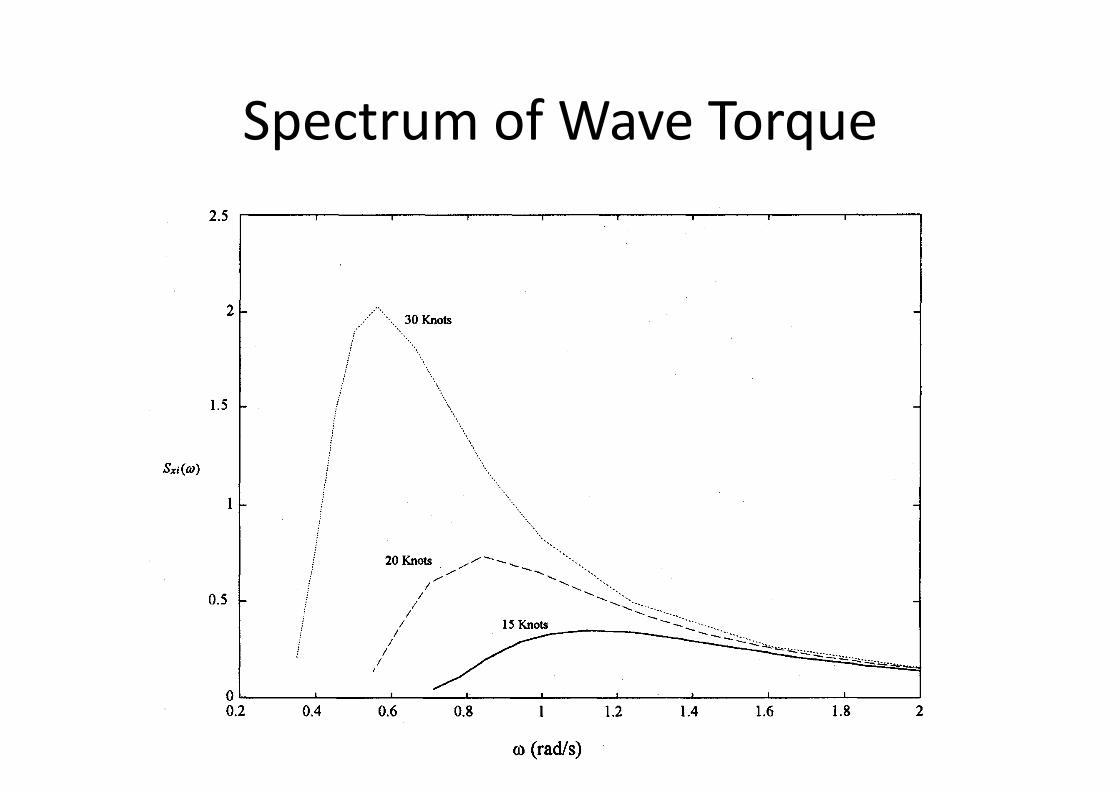
E. Model of the Waves In the system being considered, the waves are modeled as an

external disturbance torque, proportional to their slope. Several models of wave signals exist in literature 181; in this work the disturbance torque generated by the waves has been modeled as a stochastic signal whose spectrum is given by the following relationship formulated by Pierson and Kitaigorodskii 111 :

where g is the gravity constant, a and p are two constant parameters, and v is the wind speed. To represent the worst conditions for the roll, the waves have been considered as normal to the direction of navigation. In Fig. 6 the magnitude of the spectrum for three different wind conditions is shown.

Iv. IDENTIFICATION FROM EXPERIMENTAL DATA To experimentally validate the previously described model

of the system, several tests were made on the ship. The measurements were performed in calm sea, with the ship at a constant speed of 35 knots, by applying a square wave to the input of the electro-hydraulic system. The response of the ship in terms of roll-angle variation and wing-angle variation was acquired and stored by a data acquisition unit with a sample time of 50 ms. In this way it was possible to identify, by using a least-square error identification algorithm [ll], both the transfer function of the electro-hydraulic system and the transfer function of the ship [9], [lo]. A first-order model was sufficient for the electro-hydraulic system and the results obtained confirmed what was predicted in Section III- C from physical considerations. In Fig. 7 a comparison is made between the wing angle measured and the model output identified for a test input signal showing the reliability of the model.

To estimate the transfer function between the applied torque (assumed for these test conditions to be proportional to the wing angle) and the roll angle of the ship, it was necessary to identify two different models for the rise and descent phases of the wings. In fact, as can be observed from the particular response reported in Fig. 8, the behavior of the ship is rather different in these two situations. This nonlinear behavior is presumably due to the rapid variation in the position of the center of gravity and the center of buoyancy when the wings

20 IEEE TRANSACTTONS ON CONTROL SYSTEMS TECHNOLOGY, VOL. 4, NO. 1, JANUARY 1996

Waves Wings

U oil angle

Fig, 3. Block diagram of the model.

Fig, 4. A cross section of the stern of the ship.

corresponding torque C, can be approximated as

C, = Kp@. (4)

The range of variation of the dipping angle is between -18 degrees and $18 degrees.

It should be observed that to assume the ship sailing at a constant speed is not an unreasonable hypothesis, considering that most of the time during typical navigation the cruising speed is maintained.

C. Electro-Hydraulic System Model The two arms with the two wings are moved by means of

two identical electro-hydraulic systems to generate a variable torque. Each system is made up of an electro-valve which regulates the flow of high-pressure oil to either side of a cylinder. The resulting difference in pressure on a piston contained inside the cylinder causes motion of a shaft connected to the wing.

In Fig. 5 a block diagram of the electro-hydraulic system is given. From this scheme and from the physical data of the system, it follows that the first-order transfer function between the input voltage to the system V h and the wing angle a, given by

(5)

is a good linear approximation of the electro-hydraulic system.

D. Gyroscope A Gyroscope was adopted as roll-angle transducer. This

device generates a voltage reference proportional to the roll angle, following the equation

KOZZ = K g y r o Q ' r o l l . (6 )

E. Model of the Waves In the system being considered, the waves are modeled as an

external disturbance torque, proportional to their slope. Several models of wave signals exist in literature 181; in this work the disturbance torque generated by the waves has been modeled as a stochastic signal whose spectrum is given by the following relationship formulated by Pierson and Kitaigorodskii 111 :

where g is the gravity constant, a and p are two constant parameters, and v is the wind speed. To represent the worst conditions for the roll, the waves have been considered as normal to the direction of navigation. In Fig. 6 the magnitude of the spectrum for three different wind conditions is shown.

Iv. IDENTIFICATION FROM EXPERIMENTAL DATA To experimentally validate the previously described model

of the system, several tests were made on the ship. The measurements were performed in calm sea, with the ship at a constant speed of 35 knots, by applying a square wave to the input of the electro-hydraulic system. The response of the ship in terms of roll-angle variation and wing-angle variation was acquired and stored by a data acquisition unit with a sample time of 50 ms. In this way it was possible to identify, by using a least-square error identification algorithm [ll], both the transfer function of the electro-hydraulic system and the transfer function of the ship [9], [lo]. A first-order model was sufficient for the electro-hydraulic system and the results obtained confirmed what was predicted in Section III- C from physical considerations. In Fig. 7 a comparison is made between the wing angle measured and the model output identified for a test input signal showing the reliability of the model.

To estimate the transfer function between the applied torque (assumed for these test conditions to be proportional to the wing angle) and the roll angle of the ship, it was necessary to identify two different models for the rise and descent phases of the wings. In fact, as can be observed from the particular response reported in Fig. 8, the behavior of the ship is rather different in these two situations. This nonlinear behavior is presumably due to the rapid variation in the position of the center of gravity and the center of buoyancy when the wings

Spectrum of Wave Torque

FORTUNA AND MUSCATO: ROLL STABILIZATION SYSTEM 21

Controller VII Servwalve ; - -- - - - - - - - -- - output - 1 -

Wing angle cp

Piston

Vh -4 I

Transducer

Fig. 5. Block diagram of the hydraulic actuator.

2.5

2

1.5

Sxi (0)

1

0.5

0 0.2 0.4 0.6 0.8 1 1.2 1.4 1.6 1.8 2

o (rads) Fig. 6. Wave spectrum for different wind speeds.

are subjected to rapid movements, while the hydrodynamic force appears with a small lag. More specifically, during the rise phase nonminimum phase behavior was observed. To overcome such a problem two distinct ARMAX models were identified using the least-square error method [ll]; for the rise phase a fifth-order model was obtained, while for the descent phase a fourth-order model was sufficient to get a good approximation. In Figs. 9 and 10 comparisons are made between the output of the identified and the measured system for the rise and descent phases, respectively.

The self oscillations, referring to the first time steps of the identified model of Fig. 9, indicate that a fifth-order model is too high, even if this gave the smallest least-square errors.

An analysis of the poles and zeros maps of the two models has shown that both have a dominant pole pair with a damping ratio M 0.57 and an angular frequency wn M 1.37 rads. These data show good agreement with those predicted by physical considerations. The model identified for the rise phase

also has a pair of unstable zeros, but the effect of these zeros only appears in a frequency range that will not be excited by the control system. In other words, even if the ship model appears to be nonlinear for the test signal that we adopted for the identification, for the reasons that have been previously explained, it has been observed in several tests that this effect will disappear under the typical working conditions of the system, when the wings will never be subjected to such rapidly varying step commands.

v. DESIGN OF A LEAD CONTROLLER

As a first step in the design of a compensator, a proportional lead controller was established. This was due to the fact that it was possible to implement this compensator very easily using analog devices without changing the existing hardware too much. Such a compensator allowed the performance of the whole roll stabilization system to be tested to facilitate stating the specifications for more sophisticated compensators. The


dB

Fig. 11. Frequency response of the transfer function between the waves and the roll angle: (-) open loop and (- - -) closed loop

0 10 20 30 40 50 60 70 80 90 100 time (s)

Fig. 12. Roll angle without the control system.

while in Fig. 13 a measurement of the roll with the control system working is shown. It can be observed that the maximum roll deviations of the ship are strongly attenuated.

VI. ADAPTIVE LQ CONTROLLER A single linear controller cannot exploit to the utmost all

the performance of the roll reduction system. The maximum torque generated by the two wings is bounded, and very strong roll oscillations cannot be greatly attenuated. In this way the maximum open-loop gain, corresponding to the maximum

closed-loop wave disturbance rejection, must also be bounded. A controller designed for heavy sea conditions to avoid saturation will result in a small gain. By adopting the same controller when the sea is calm, the potentiality of the system would not be fully exploited.

To get the best performance from the roll-reduction system for all sea conditions, an adaptive LQ controller of the gain scheduling type has been designed [5], [12], [13].

A state-space model of the ship was derived adopting the roll, the rate of the roll, and the wing angle as state variables. This choice was suggested by physical considerations and by

Without and With Control


dB

Fig. 11. Frequency response of the transfer function between the waves and the roll angle: (-) open loop and (- - -) closed loop

0 10 20 30 40 50 60 70 80 90 100 time (s)

Fig. 12. Roll angle without the control system.

while in Fig. 13 a measurement of the roll with the control system working is shown. It can be observed that the maximum roll deviations of the ship are strongly attenuated.

VI. ADAPTIVE LQ CONTROLLER A single linear controller cannot exploit to the utmost all

the performance of the roll reduction system. The maximum torque generated by the two wings is bounded, and very strong roll oscillations cannot be greatly attenuated. In this way the maximum open-loop gain, corresponding to the maximum

closed-loop wave disturbance rejection, must also be bounded. A controller designed for heavy sea conditions to avoid saturation will result in a small gain. By adopting the same controller when the sea is calm, the potentiality of the system would not be fully exploited.

To get the best performance from the roll-reduction system for all sea conditions, an adaptive LQ controller of the gain scheduling type has been designed [5], [12], [13].

A state-space model of the ship was derived adopting the roll, the rate of the roll, and the wing angle as state variables. This choice was suggested by physical considerations and by

FORTUNA AND MUSCATO: ROLL STABILIZATION SYSTEM 25

0 10 20 30 40 50 60 70 80 90 100 time (s)

Fig. 13. Roll angle with the control system activated.

the fact that all three variables are easily measurable in the system.

The LQ index minimized was

where z is the state vector, while U is the input of the electro- hydraulic system, and Qz is a nonnegative definite weighting matrix. With this choice, the robustness of the regulator is ensured by the fact that such an optimal regulator always guarantees a phase margin of 60 degrees [12].

Several different classical LQ controllers were designed, one for each sea condition, by appropriately choosing the Qi matrices and computing the corresponding LQ-gain vectors [2]. The adaptation was performed by changing the values of the gain vector computed for the corresponding sea conditions. A neural network was adopted to interpolate the suitable gains for the controller at any time from an estimation of the sea conditions.

To test the performance of these controllers, the mean square errors of the roll of the ship were computed for the same disturbance signal for the system in open loop with the lead controller and with the LQ-regulator for three different wind speeds. The chart in Fig. 14 summarizes these results, showing the better performance of the LQ regulators with respect to the classical lead controller. This figure reports the mean square errors of the roll of the ship computed according to the formula

tf .-," = 1 [Q(t ) l2 d t (9)

where, for the simulations considered, it was assumed that t f = 80 S.

It must be observed that sea conditions usually change very slowly with respect to the dynamic of the system, so

the adaptation system does not need to have a fast response. The estimation of sea conditions is performed by using a measurement of the roll motion of the ship. To get a good estimate that is not affected by disturbances, long-time measurements are needed. A multilayer perceptron neural network [ 141 was used to estimate the sea conditions and interpolate the corresponding gain values of the LQ regulator. The choice of a neural network as an interpolator was suggested by the good performance that this kind of device has given in interpolating arbitrary unknown functions [15]. Moreover, in the future they could allow a continuous multidimensional map between different input signals to be obtained, denoting the conditions of the sea and ship (such as wind velocity, wave height, ship speed, ship load, etc.) and the optimal regulator gains.

In Fig. 15 a block diagram of the adaptive controller is shown, while Fig. 16 summarizes the role of the neural network. As the input of the neural network a sequence of delayed roll measurements were considered

i n p u t ( k ) = [ Q ( k ) , Q ( k - l), . . . Q ( k - n)] (10)

while the outputs were the three gains of the LQ controller. To compute the input-output patterns for the learning phase

of the network, six sets of LQ gains, corresponding to six different sea conditions, were computed. Several simulations were performed for each of these regulators with various simulated sea conditions. Then the pattems were formed by taking a time series of the roll as input and the LQ gains corresponding to the simulated sea state as output. After a trial-and-error optimization phase, a three-layer perceptron with 15 input neurons (corresponding to n = 14), 10 hidden neurons, and three outputs was chosen. The learning phase was completed by using a modified back propagation algorithm [ 161 performed on the pattern signal previously generated.

Open Loop vs Lead vs LQR 26

- m// angle

roll angle rate

IEEE TRANSACTIONS ON CONTROL SYSTEMS TECHNOLOGY, VOL. 4, NO. 1, JANUARY 1996

Gyro < I -

BLead Controller

15 Knots 20 Knots 30 Knots

Fig. 14. Comparison between the mean square errors for three different conditions.

LQ Gains Neural / Network \

Waves Wings

I I I - I

Fig. 15. Block diagram of the adaptive LQ controller.

Fig 16 The role of the neural network in the control block

Regulator gains

Extensive simulations of this adaptive controller were performed to test the capabilities of such a system. Fig. 17 shows a particular simulation of the roll-angle behavior where three different sea conditions are simulated successively.

As can be observed, the controller automatically and gradu- ally switches between the three different conditions. Moreover, it can be seen that the amount of relative roll reduction with respect to the open-loop situation is different for the three situations. In fact, for the 30 knots case, for example, it is not possible to obtain the same amount of reduction in dB as in the 15 knots case. This is mainly due to the fact that in this latter case larger regulator gain values are allowed than those adopted in the first situation, where saturation constraints limit the maximum value of the relative reduction. Moreover, it should be observed that in a real situation such rapid weather changes are very improbable.

VII. CONCLUSIONS In this paper the various steps involved in the design of

an automatic roll reduction system have been presented. The roll damping system consists of two auxiliary automatically controlled wings. Even if it is very difficult to perform a


State-‐space strategies -‐ “Modern Control” •  System equaGons are described in matrix form. •  Most fundamental are the state variables: A set of parameters

that completely describes everything worth knowing about the system. –  For example posiGon and velocity of a moving body

•  Using measurements of the outputs, the system state can be computed -‐ observers

•  Using the system state, control strategies can be devised to achieve desired performance. –  Pole placement –  OpGmal controllers

•  AbracGve for mulG-‐input mulG-‐output (MIMO) systems


State Space Modelling

•  Using the state space approach, we represent a system by a set of n first-‐order differenGal equaGons:

•  The output of the system is expressed as:

x -‐ state vector y -‐ output vector u -‐ input vector

A -‐ state matrix B -‐ input matrix C -‐ output matrix D -‐ feedthrough or feedforward matrix (ocen zero)

State Space Modelling

•  We can draw a block diagram describing the general State Space Model


Stability in State Space

•  The transfer function is

•  Poles occur when (sI-A) is not an invertible matrix.

•  i.e. when det(sI-A) = 0 •  For what s does this occur? Eigenvalues of A

Dr Ian R. Manchester Amme 3500 : State Space

€

Y (s)U(s)

= C(sI − A)−1B +D


State Space Control

•  We can represent a general state space system as a Block Diagram.

•  If we feedback the state variables, we end up with n controllable parameters.

•  State feedback with the control input

u=-‐Kx +r.

* N.S. Nise (2004) “Control Systems Engineering” Wiley & Sons


State Space Control

•  We can then control the pole locaGons by finding appropriate values for K

•  This allows us to select the posiGon of all the closed loop system roots during our design.

•  There are a number of methods for selecGng and designing controllers in state space, including pole placement and opGmal control methods via the Linear QuadraGc Regulator algorithm.

State Space Control

•  Seing u=-‐Kx+r yields

•  Rearranging the state equaGon and taking LT yields

•  Select values of K so that the eigenvalues (root locaGons) of (A-‐BK) are at a parGcular locaGon


Dr Ian R. Manchester Amme 3500 : State Space

State Feedback Control

THEOREM: The following statements are equivalent:

1. For any time T > 0 there exists a control signal u(t) driving the state from any initial state x(0) to any final state x(T).

2. For any choice of closed loop pole locations, there exists a constant gain matrix K such that u=-Kx has the desired poles.

3. The matrix [B AB A2B… An-1B] is full rank

Steady State Error

•  Full state feedback does not directly address the issue of steady state error

•  A common strategy is to feedback the output and add additional state variables

Dr Ian R. Manchester Amme 3500 : State Space 2


Steady State Error

•  Looking at the previous diagram, we find

•  We can augment the state equations yielding


Steady State Error

•  But

•  So

•  We can now choose gains to yield desired pole locations and zero steady state error


€

u = −Kx +KE xN = − K KE[ ]xxN

⎡

⎣ ⎢

⎤

⎦ ⎥

€

˙ x ˙ x N

⎡

⎣ ⎢

⎤

⎦ ⎥ =

A −BK BKe

−C 0⎡

⎣ ⎢

⎤

⎦ ⎥

xxN

⎡

⎣ ⎢

⎤

⎦ ⎥ +

01⎡

⎣ ⎢ ⎤

⎦ ⎥ r

y = C 0[ ]xxN

⎡

⎣ ⎢

⎤

⎦ ⎥

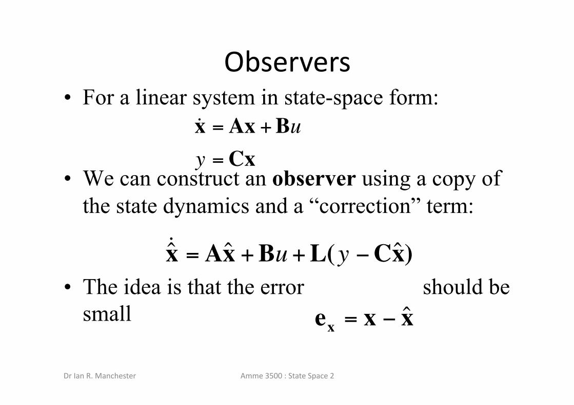
•  For a linear system in state-space form:

•  We can construct an observer using a copy of the state dynamics and a “correction” term:

•  The idea is that the error should be small

Observers

Dr Ian R. Manchester Amme 3500 : State Space 2 €

ˆ ˙ x = Aˆ x + Bu + L(y −Cˆ x )

€

ex = x − ˆ x

€

˙ x = Ax + Buy = Cx

Observers •  Let us examine the dynamics of the error:

•  I.e. if the matrix (A-LC) is stable, then any initial error goes to zero exponentially


€

˙ e x = ˙ x − ˆ ˙ x = Ax + Bu −Aˆ x −Bu −L(y −Cˆ x )= (A −LC)x − (A −LC)ˆ x = (A −LC)ex

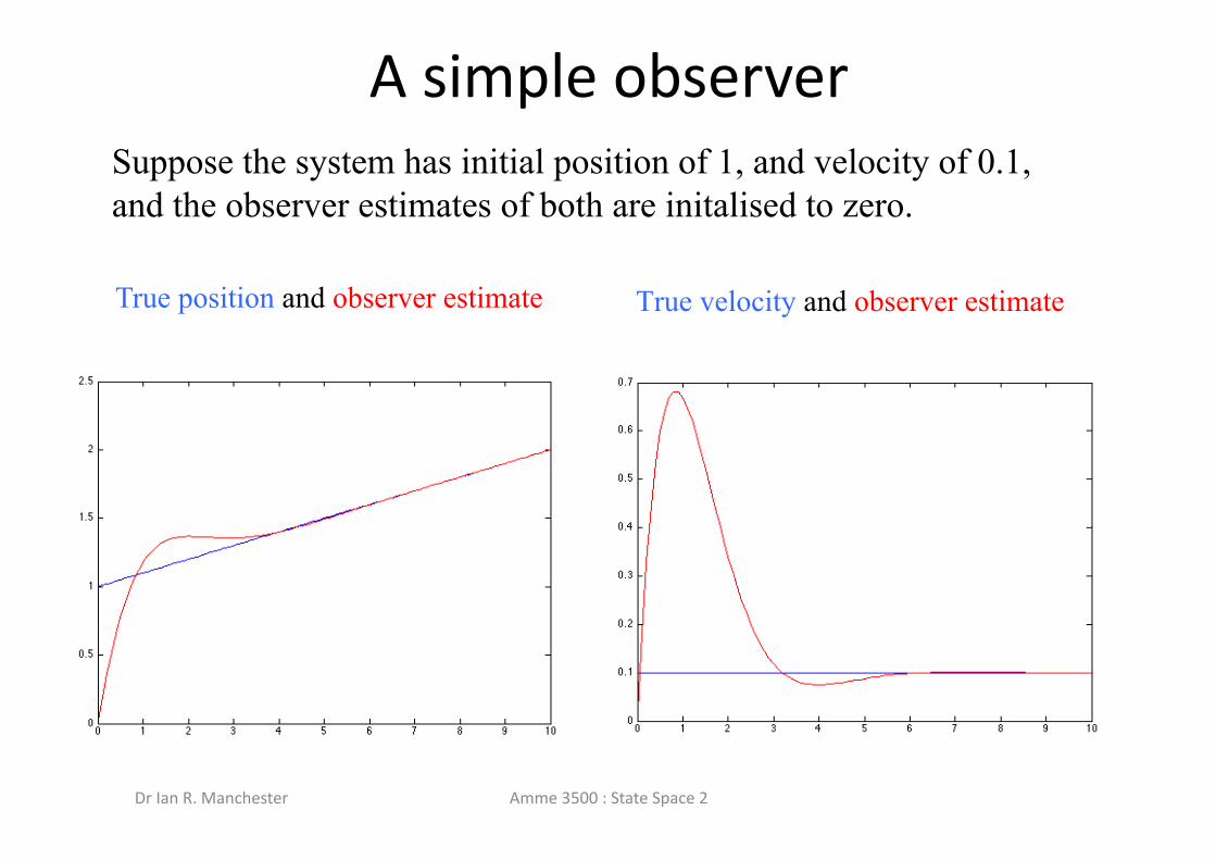
A simple observer

True position and observer estimate


Suppose the system has initial position of 1, and velocity of 0.1, and the observer estimates of both are initalised to zero.

True velocity and observer estimate

Observability •  In an analgous manner to controllability, we

can also check the observability of a system using the observability matrix


Output Feedback Control •  By designing a state-feedback controller, and

an observer to estimate the state, one can design a controller that only depends on the output of the system:


Output-‐Feedback Control



TransformaGon Suppose x=Tz, with T invertible, then

Which gives a way of constructing T:


€

Oz =

CTCT(T−1AT)

CT(T−1AT)(T−1AT)

CT(T−1AT)(T−1AT)(T−1AT)

⎡

⎣

⎢ ⎢ ⎢ ⎢ ⎢ ⎢

⎤

⎦

⎥ ⎥ ⎥ ⎥ ⎥ ⎥

=

CCACA2

CAn−1

⎡

⎣

⎢ ⎢ ⎢ ⎢ ⎢ ⎢

⎤

⎦

⎥ ⎥ ⎥ ⎥ ⎥ ⎥

T =OxT

€

T =Ox−1Oz

Theorem


THEOREM: The following statements are equivalent: 1. Over any time interval [0, T], it is possible to

reconstruct the state x(t) based on knowledge the input u(t) and the output y(t).

2. For any choice of observer pole locations, there exists a constant observer gain matrix L such that A-LC has the desired poles.

3. The observability matrix has full rank


What about the Exam???

•  You should be familiar with the concepts reviewed in this lecture – Modelling of dynamic systems – SpecificaGon of second order systems – Root Locus – Bode Plots – Design and properGes of PID (and variants), Lead and Lag controllers

– State Space Modelling and Design


What about the Exam???

•  You will not be required to find roots of polynomials higher than second order.

•  You will be provided with a selected set of equaGons you may require for solving the problems

•  In order to prepare I would suggest that you –  Review the assignment quesGons, making sure you understand the material covered this semester

–  Look over previous years’ exams

amme$3500/5501$:$$ system$dynamics$&$control$...

Documents