n

4

Dynamic Analysi

and Forces

4.1 INTRODUCTION

In previous chapters, we studied the kinematic position and differential motions ofrobots. In this chapter, we will look at the dynamics of robots as it relates to acceler­ations, loads, and masses and inertias. We will also study the static force relation­ships of robots.

As you remember from your dynamics course, to be able to accelerate a mass,we need to exert a force on it. Similarly, to cause an angular acceleration in a rotat­ing body, a torque must be exerted on it (Figure 4.1), as in

and 2: T = I· a. (4.1)

To be able to accelerate a robot's links, it is necessary to have actuators thatare capable of exerting large enough forces and torques on the links and joints tomove them at a desired acceleration and. velocity. Otherwise, tbe link may not bemoving fast enough, and thus the robot will lose its positional accuracy. To be ableto calculate how strong each actuator must be, it is necessary to determine the dy­namic relationships that govern the motions of the robot. These equations are theforce-mass-acceleration and the torque-inertia-angular acceleration relation­ships. Based on these equations and considering the external loads on the robot, thedesigner can calculate the largest loads to which the actuators may be subjected andthereby design the actuators to be able to deliver the necessary forces and torques.

In general, the dynamic equations may be used to find the equations of motionof mechanisms. This means that knowing the forces and torques, one can figure outhow a mechanism will move. However, in our case, we have already found the equa­tions of motions; besides, it is practically impossible to solve the dynamic equations

119

120 Chapter 4 Dynamic Analysis and Forces

Figure 4.1 Force-mass-accelerationand torque-inertia-angular accelerationrelationsl1ips for a rigid body.

\,'

of robots in all but the simplest cases. Instead, we will use these equations to findwhat forces and torques may be needed to induce desired accelerations in therobot's joints and links. These equations are also used to see the effects of differentinertial loads on the robot and, depending on the desired accelerations, whethercertain loads are important. For example, consider a robot in space. Although ob­jects are weightless in space, they do have inertia. As a result, the weight of objectstllat a robot in space may handle may be trivial, but its inertia is not. So long as themovements are very slow, a light robot may be able to move very large loads inspace with little effort. This is why the robot used with the Space Shuttle program isvery slender; but handles very large satellites. The dynamic equations allow the de­signer to investigate the relationship between different elements of the robot anddesign its components appropriately.

In general, techniques such as Newtonian mechanics can be used to find thedynamic equations for robots. However, due to the fact that robots are three­dimensional, multiple-degree-of-freedom mechanisms with distributed masses, it isvery difficult to use Newtonian mechanics. Instead, one may opt to use other tech­niques such as Lagrangian mecllanics. Lagrangian mechanics is based on energyterms only and thus in many cases is easier to use. Although Newtonian mechanics,as well as other techniques, can be used for this derivation, most references arebased on Lagrangian mechanics. In this chapter, we will briefly study Lagrangianmechanics with some examples, and then we will see how it can be used to solve forrobot equations. Since this course is primarily intended for undergraduate stUdents,the equations will not be completely derived, but only the results will be demon­strated and discussed. Interested students are encouraged to refer to other refer­ences for more detail [1,2,3,4,5,6,7].

4.2 LAGRANGIAN MECHANICS: A SHORT OVERVIEW

Lagrangian mechanics is based on the differentiation of the energy terms with re­spect to the system's variables and time, as shownlJf.xt. For simple cases, it may takelonger to use this technique than Newtonian mechanics. However, as the complexi­ty of the system increases, the Lagrangian method becomes relatively simpler touse. The Lagrangian mechanics is based on the following two generalized equations,one for linear motions, one for rotational motions. First we will define a Lagrang­ian as

L = K - P, (4.2)

where L is the Lagrangian, [( is the kinetic energy of the system, and P is the poten­tial energy of the system. Then

Section 4.2 Lagrangian Mechanics: A Short Overview .121

F = ~ (aL) aL(4.3), at ax; ax; ,

T = ~eL)

aL(4.4)

I at ae; ae; ,

where Fis the summation of all external forces for a linear motion, T is the summa­tion of all torques in a rotational motion, and and x are system variables. As a result,to get the equations of motion, we need to derive energy equations for the system,and then differentiate the Lagrangian according to Equations (4.3) and (4.4). Thefollowing three examples demonstrate the application of Lagrangian mechanics inderiving equations of motion. Notice how the complexity of the terms increases asthe number of degrees of freedom (and variables) increases.

Example 4.1

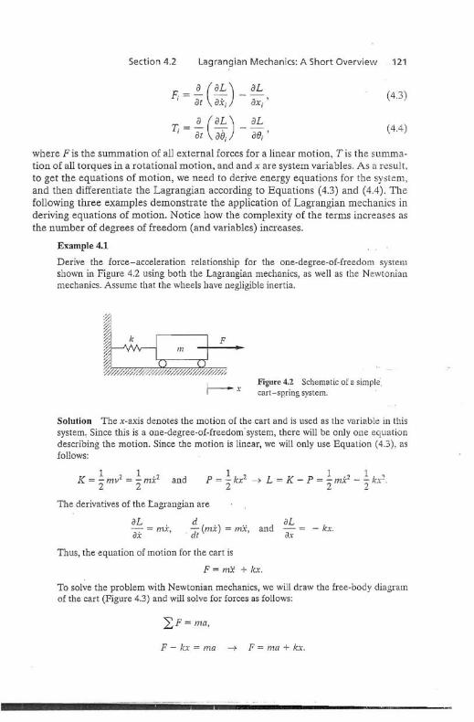
Derive the force-acceleration relationship for the one-degree-of-freedom systemshown in Figure 4.2 using both the Lagrangian mechanics, as well as the Newtonianmechanics. Assume that the wheels have negligible inertia.

'-;'l

~/'/-~ k F~r--v'Y\"'---1~ L.,..,c---.,......J

::?/'//'z<;/0/~1'/ir/Y/Y.%///),W~/,'~·»

f--xFigure 4.2 Schematic of a simpkcart-spring system.

Solution The x-axis denotes the motion of the cart and is used as the variable in thissystem, Since this is a one-degree-of-freedom system, there will be only one equationdescribing the motion. Since the motion is linear, we will only use Equation (4.3). asfollows:

The derivatives of the Lagrangian are

aL .ax = mx,

ddt(mx)=mx, and

aLax

- kx.

Thus, the equation of motion for the cart is

F = mx + /ex.

To solve the problem with Newtonian mechanics, we will draw the free-body diagramof the cart (Figure 4.3) and will solve for forces as follows:

:LF= ma,

F - lex = l11a --7 F = 111{/ + lex.

Solution In tbis problem, there are two degrees of freedom. two coordinates x and e,and there will be two equations of motion: one for the linear motion of the system andone for the rotation of the pendulum.

I :-rma

F

Figure 4.4 Schematic of a cart-/112 pendulum system,

vi, = (~t + lil cos 8)2 + (lil sin W..~

1 . 1· 2Kpendllium = '2 m2(~t + Ie cos 8)2 + '2 m2 (Ie sin 8) ,

K = Kcar• + J(pendlllum,

kx~_~F

Figure 4.3 Free-body diagram for the spring-cart system.

Dynamic Analysis and Forces

This is exactly what we expected. For this simple system, it appears that New-tonian mechanics is simpler.

Example 4.2

Derive tbe equations of motion for the two-degree-of-freedom system shown in Fig­ure 4.4.

and

Thus,

The kinetic energy of the system is comprised of the kinetic energy of the cart.and of the pendulum. Notice that the velocity of the pendulum is the summation ofthe velocity of the cart and of the pendulum relative to the cart, or

Vp = Vc + Vp/c = xi + l8 cos ei + l8 sin e1 = (* + 18] cos 8)i + l8 sin e1.

122 eha pter 4

-

The derivatives and the equation of motion related to the linear motion are

1. ) 1. , ',' 1.,L = K - P = 2" (1111 + I11z)x- + 2" I11z(l-e- + Zlex cos e) - 2"lcx- - Jn2g/(1 - cos 8).

Likewise, the potential energy is the summation of the potential energy in thespring and in the pendulum, or

(t. The La-

Lagrangian Mechanics: A Short Overview 123

1.) (~ )p = 2" lex- + megl 1 - COS 8 .

Section 4.2

aL---:- = (1111 + 1112)5: + 111218 cos 0,ax

Notice that the zero-potential-energy line (datum) is chosen at egrangian is

dd (aL) = (1111 + 1112)::( -I- m./ecose - 1112182sinfJ,t ax

!!.- (aL) = I11,Lze + l11ol.X: cos 0 - In.,I.tO sin e,dt ae - - -aL .- = -m.,gfsin e - In,lfh sin e,ao· -

F = (111[ -I- 1112).i + 11121e cos f) - m.2le2sin e -I- lex.

For the rotational motion, it is

aL "-:- = 111,/-e + m.21x cos e,ae -

[lex ]

+ 1112g1 sin (J .

- lex,aLax

T = Jn2f2e + I11Ix cos e + 1112g1 sin fl.

If we write the two equatiqns of motion in a matrix form, we get

F= (1111 + I11z)i + /77.zle cos e - /77.21i:J2sine + lex,

T = 1112/2e + I11 zli cos e + I11zg1 sin e,(4.5)

[FT

] = [ml + 11"/.2 11121cos 0] [~] + [0 1Tl21 Sill e] [x:]m2/CaSe 1112/Z e ° ° _e-

....;~y:

Example 4.3

Derive the equations of motion for the two-degree-of-freeclom system shown inFigure 4.5.

Solution Notice that this example is somewhat more similar to a robot, except thalthe mass of each link is assumed to be concentrated at the end of each link and that

there are only two degrees of freedom. However, in this example, we will see manymore acceleration terms, such as we would expect to see with robots, such as centrip­etal accelerations and Coriolis accelerations.

124 Chapter 4 Dynamic Analysis and Forces

y

or----~x

A1111

~2/2

1n2

BFigure 4.5 A two-link mechanism withconcentrated masses,

We will follow the same format as before. First, we calculate the kinetic andpotential energies of the system:

where

To calculate /(2, first we will write the position equation for 1n2 and then dif­ferentiate it for the velocity of m2:

{

X 2 = I,sin 8, + 12 sin (8 j + 82) = 11S1 + 12S12,

Y2 = - I, C1 - 12C12'

{X2 = llC1e, + 12C12(e\ + ~2)'

Y2 = 115\ 81 + 12S12 (81 + 82), '~

Sioce Vl = Xl + y2 , we get

v~ = ItiJt + g(et + e~ + 2e\e2) + 21112(ei + e1( 2 )(C\CI2 + 5 15\2)

= Ite~ + I~(et + e~ + 28182) + 21112 C2(8i + 8182),

Then the kinetic energy for the second mass is

1 2'2 1 2'2 '2 ", '2' ./(2 = "211121j8, + "2 1112 [2(81 + 82 + 28182) T 1n211[2C2(81 + 8182),

·····.f

Section 4.2

and the total kinetic energy is

Lagrangian Mechanics: A Short Overview 125

1K = -(m1 +

2..,' 1 I

I-I' e, + mil? + e~ +- 2 - - ~+ +

The potential energy of the system can be written as

PI = m [gil Cl ,

P PI + P2 =

Notice that in this case, the datumof rotation "0."

is chosen at the axis

The for the system is

L K-P 12

+

The derivatives of the Lagrangian are

aL= (m'l +

+ + +

+aLael

From Equation (4.4), the first equation of motion is

Similarly,

+ + In21112C2]

+

aL

ae2

d aLdt

+

+

+

+

+

+

126 Chapter 4 Dynamic Analysis and Forces

Writing these two equations in a matrix form, we get

[TTzI ] = [(177 1+ m.z)l~ + ml1~ + 217721j12C2 m21~ + m/112C2][~1]

(mIi + 11721112CJ 171 21'5. O2

+ [(In, + 1712)gl,SI + 1712gl2SI2].m2f512S12

Example 4.4

Using the Lagrangian method, derive the equations of motion for the two-degree-of­freedom robot arm, shown in Figure 4.6. The center of mass for each link is at the cen­ter of the link. The moments of inerti, are II and 12 •

Figure 4.6 A two-degree-of-freedomrobot arm.

Solution The solution of this example robot arm is in fact similar to the solution ofExample 4.3. However, in addition to a change in the coordinate frames, the two linkshave distributed masses, requiring the use of moments of inertia in the calculation ofthe kinetic energy. We will follow the same steps as before. First, we calculate the ve­locity of the center of mass of link 2 by differentiating its position:

Xo = I,C, + 0.512C11 -> -to = -lfS,9, - 0.512S12 (9, + 92),

Yo = IISI + 0.512S12 .~ Yo = I,CI9, + 0.512C'2(9, + (h)·

Therefore, the total velocity of the center of mass of link 2 is

Vb = ·:i:b + jib= eT (if + O.251~ + l112C2) + e~ (O.251~) + ele2(O.51~ + ljI2C2)· (4.7)

The kinetic energy of the total system is the sum of the kinetic energies oflinks 1 and 2. Remembering the formula for finding kinetic energy for a link rotat­ing about a fixed axis (for link 1) and about the center of mass (for link 2), we have

Section 4.3 Effective Moments of Inertia 127

., (1 ') .. (1 ,1 )+(J:; -6m,l:; + (JJ(J, -m,I:;+-m,III,C, .- "- - 3 -- 2 - --

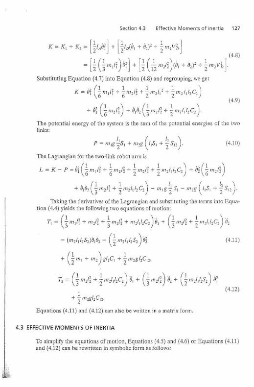
The potential energy of the system is the sum of the potential energies of the twolinks:

(4.10)

.,(1 ')+ (Jz 6Jn21'j

. . (1 ,1 ) Ij (12 )+eje, -171,I,+-m,ll/,C, -m,g-5 j -m.,g 115 1 +-51,."\3 • - 2 - - - 2 - \ 2-

Taking the derivatives of the Lagrangian and substituting the terms into Equa­tion (4.4) yields the following two equations of motion:

(1 2 ,1 2 ) .. ,(1 2 1 )..T] = - mj/l + m.,l-l + - m,12 + m,II/,C, ej T - m,l, + - m,III,C, (J,3 - 3· _. . 3·- 2 - - - -

- (m.2 /j I2S2)e/32- (im2IjI252)i:J~

+ (~/)1.1 + m2)gllCI + imZgl2CI2,

1+ - m,gl,C j7 •2 - - -

Equations (4.11) and (4.12) can also be written in a matrix form.

4.3 EFFECTIVE MOMENTS OF INERTIA

(4.11)

(4.12)

To simplify the equations of motion, Equations (4.5) and (4.6) or Equations (4.11)and (4.12) can be rewritten in symbolic form as foJlows:

128 Chapter 4 Dynamic Analysis and Forces

(4.13)

(4.14)

In this equation, which is written for a two-degree-of-freedom system, acoefficient in the form of D i ,. is known as effective inertia at joint i, such that an ac­celeration at joint i causes a torque at joint i equal to D)i,., whereas a coefficient inthe form Dij is known as coupling inertia between joints i and j as an acceleration atjoint i or j causes a torque at joint j or i equal to Di/ii or Djiej. Dijj8J terms representcentripetal forces acting at joint i due to a velocity at joint j. All terms with 8182 rep­resent Coriolis accelerations, and when mUltiplied by corresponding inertias, theywill represent Coriolis forces. The remaining terms in the form D i represent gravityforces at joint i.

4.4 DYNAMIC EQUATIONS FORMULTIPLE-DEGREE-OF-FREEDOM ROBOTS

As you can see, the dynamic equations for a two-degree-of-freedom system is muchmore complicated than a one-degree-of-freedom system. Similarly, these equationsfor a multiple-degree-of-freedom robot are very long and complicated, but can befound by calculating the kinetic and potential energies of the links and the joints, bydefining the Lagrangian, and by differentiating the Lagrangian equation with re­spect to the joint variables. The next section presents a summary of this procedure.For more information, please see [1,2,3,4,5,6,7].

4.4.1 Kinetic Energy

As you may remember from your dynamics course [8], the kinetic energy of a rigidbody with motion in three dimensions is (Figure 4.7(a»

1 - 1 -J( = 2' mV 2 + 2' w.he,

where he is the angular momentum of the body about G.

,,,

cG

(a)

v

(b)Figure 4.7 A rigid body in three­dimenslonaJ motion and in piane motion.

Section 4.4 Dynamic Equations for Multiple-Oegree-of-Freedom Robots 129

The kinetic energy of a

K

in planar motion

1 -? 1 - "- mV- + I(v~.

2 2

4.7 (b)) "UUJL!-,"LU,",'-' to

(4.15)

Thus, we will need to derive expressions for of a point(e.g., the center of mass G), as well as the moments of inertia.

The velocity of a along a robot's link can be defined by GlIlCen:;l1tlarlll1gthe position equation the point, which, in our notation, is expressed by a framerelative to the robot's base, RTp . Here, we will use the D-H transformation matrices

to find the terms for along the robot's links. In 2, wedefined the transformation between the hand frame and the base frame of the robotin terms of the A matrices as

RTI-J =

For a six-axis robot, this '-'\.lI.lCU.1V.l1 can be written as

Referring to Equation (2.52), we see that the derivative of an Ai matrix for arevolute joint with respect to its variable (Ji is

-se;CCti

aA; a [ COiCCt; ceiSCti---ai = ae· 0 Sai CCtiI I

0 0 0

-sei -Ce;CCti CeiSCticel seiSa!0 0 00 0 0

a!CeiaiSOi

di

1

oo

However, this matrix can be broken into a constant matrix Qi and the Ai matrixsuch that

-sa; -cejCCtj cejSajcei saiSaj ajCej

0 0 0 0

0 0 0 0

[~-seiCai a;CB]

(4.18)-1 0 0 cel seiSai0 0 0 S8; ce;CCti C();SCti L1;SfJ j

XSai eli '0 0 0 0 Cai

0 0 0 0 0 0 1

or

= Q;A!.

144 Chapter 4 Dynamic Analysis and Forces

each joint to drive the robot with desired velocity and accelerations. They can alsobe used to choose appropriate actuators for a robot,

Dynamic equations of three-dimensional mechanisms with multiple degreesof freedom such as robots are complicated and, at times, very difficult to use, As aresult, they are mostly used in simplified forms with simplifying aE.sumptions. Forexample, one may determine the importance of a particular term and its contribu­tion to the total torque or power needed by considering how large it is relative toother terms, For instance, one may determine the importance of Coriolis terms inthese equations by knowing how large the velocity terms are, Conversely, the im­portance of gravity terms in space robots may be determined and, if appropriate,dropped from the equations of motion.

In the next cl1apter, we will discuss how a robot's motions are controlled andplanned to yield a desired trajectory,

REFERENCES

1. Paul, Richard P" Robot Manipulators, Mathematics, Programming, and Control, The MITPress, 1981.

2, Shahinpoor, Mohsen, A Robot Engineering Textbook, Harper and Row, New York, 1987.

}, Asada, Haruhiko, 1. 1. E" Slotine, Robot Analysis and Control, John Wiley and Sons, NewYork,1986,

4, Sciavicco, Lorenzo, B, Siciliano, Afodeling and Control of Robot Manipulators, McGraw­Hill, New York. 1996,

5, Fu, K. S" R C Gonzalez, C S, G, Lee, Robotics: Control, Sensing, Vision, and Intelligence,McGraw-Hill. 1987,

6, Featherstone. R, "The Calculation of Robot Dynamics Using Articulated-Body Inertias,"The International Journal of Robotics Research, Vol. 2, No, I, Spring 1983, pp, 13-30,

7, Shahinpoor. M" "Dynamics," International Encyclopedia of Robotics: Applications andAutomation, Richard C Dart, Editor, John Wiley and Sons, New York, 1988, pp, 329-347,

8. Pytel, Andrew, J. Kiusalaas, Engineering Mechanics, Dynamics, 2d Edition, Brooks/ColePublishing, Pacific Grove, 1999,

9. Paul, Richard, C. N. Stevenson, "Kinematics of Robot Wrists," The International ]oLlmalofRobotics Research, Vol. 2, No, 1, Spring 1983, pp, 31-38,

10, Whitney, D, E" "The Methematics of Coordinated Control of Prosthetic Arms and Ma­nipulators," Transactions of ASME, Journal of Dynamic Systems, Measurement, andControl, 94G(4), 1972, pp, 303-309, . .:i>-

ll. Pytel, Andrew, J. K'iusalaas, Engineering Mechanics, Statics, 2d Edition, BrookslColePublishing, Pacific Grove, 1999.

12, Chicurel, Marina, "Once More, With Feeling," Stanford Magazine, March/April 2000,pp,70-73

PROBLEMS

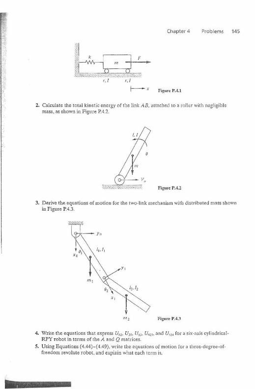
1. Using Lagrangian mechanics, derive the equations of motion of a cart with two tiresunder the cart shown in Figure PAL

F

:~:-;;-,'/,'

~)-/\f\kl'v-----i~',c

~~/X;'X~~/~/X';~~:';'///...z.,~/ 7,:;';/;"/~.

Chaptel' 4 Problems 145

r,I r, I

I--~.r Figure 1'.4.1

2. Calculate the total kinetic energy of the link AB, attached to a roller with negligiblemass, as shown in Figure PA.2.

FigureP.4.2

3. Derive the equations of motion for the two-link mechanism with distributed mass shownin Figure P.4.3.

m'2 Figure 1'.4.3

4. Write the equations that express VOl, VJ;, V5J , Vn'" and Ui )., for a six-axis cylindrical­RPY robot in terms of the A and Q matrices.

5. Using Equations (4.44)-(4.49), write the equations of motion [or a three-degree-of­freedom revolute robot, and explain what each term is.

-----

118 Chapter 3 Differential Motions and Velocities

~I

8 0 0 0 0 0 0

"~ [l1 0

l;~-3 0 1 0 0 a 0.1

a 0T.] = 0 10 0 0 0 0 Do =

-0.1

0 -1 o ' 0 1 0 0 1 o ' 0.2

0 0 1 0 0 0 1 0 0 0.2

-1 0 0 0 0 1 0

6. Calculate the T'.T21 element of the Jacobian for the revolute robot of Example 2.19.

7. Calculate the r,'],6 element of the Jacobian for the revolute robot of Example 2.19.

8. Using Equation (2.33), differentiate proper elements of the matrix to develop a set ofsymbolic equations for joint differential motions of a cylindrical robot, and write thecorresponding Jacobian.

9. Using Equation (2.35), differentiate proper elements of the matrix to develop a set ofsymbolic equations for joint differential motions of a spherical robot and write the cor­responding Jacobian.

10. For a cylindrical robot, the three joint velocities are given for a corresponding location.Find the three components of the velocity of the hand frame given the following:

j' = 0.1 in/sec, a= 0.05 rael/sec i = 0.2 in/sec, r = 15 in, ex = 30°, / = 10 in.

11. For a spherical robot, the three joint velocities ~re given for a corresponding location.Find the threecomponents of the velocity of the hand frame given the following:

I' = 2 in/sec, ~ = 0.05 rad/sec y = 0.1 rad/sec, r = 20 in, f3=60°, y = 30°.

12. For a cylindrical robot, the three components of the velocity of the hand frame are givenfor a corresponding location. Find the required three joint velocities that will generate'the given hanel frame velocity:

x = 1 in/sec, Ji = 3 in/sec, Z = 5 in/sec, a = 45°, r = 20 in, 1= 25 ill.

13. For a spherical robot, the three components of the velocity of the hand frame are givenfor a corresponding location. Find the required three joint velocities that will generatethe given hanel frame velocity:

x = 5 in/sec, y = 9 in/sec, Z = 6 in/sec, f3 = 600, r = 20 in, y = 30°.

T\V,-t~)~';- l \~

l~, ~D\

...-'I-r c· VI.--\. ~

d