discovering communicable models from earth science … · discovering communicable models from...

Discovering Communicable Models from Earth Science Data

Mark Schwabacher’, Pat Langley2, Christopher Potter3, Steven K l ~ o s t e r ~ > ~ , and Alicia T o r r e g r o ~ a ~ > ~

NASA Ames Research Center, Computational Sciences Division MS 269-3, Moffett Field, CA 94035 mark.schwabacherQarc.nasa.gov

2164 Staunton Court, Palo Alto, CA 94306 langley(9isle.org

MS 242-4, Moffett Field, CA 94035 cpotter(9gaia.arc.nasa.gov

Seaside, CA 93955

Institute for the Study of Learning and Expertise

NASA Ames Research Center, Earth Science Division

California State University Monterey Bay, Earth System Science and Policy

Abstract. This chapter describes how we used regression rules to improve upon results previously published in the Earth science literature. In such a scientific application of machine learning, it is crucially important for the learned models to be understandable and communicable. We recount how we selected a learning algorithm to maximize communicability, and then describe two visualization techniques that we developed to aid in understanding the model by exploiting the spatial nature of the data. We also report how evaluating the learned models across time let us discover an error in the data.

1 Introduction and Motivation

Many recent applications of machine learning have focused on commercial data, often driven by corporate desires to better predict consumer behavior. Yet scientific applications of machine learning remain equally important, and they can provide technological challenges not present in commercial domains. In particu- lar, scientists must be able to communicate their results to others in the same field, which leads them to agree on some common formalism for representing knowledge in that field. This need places constraints on the representations and learning algorithms that we can utilize in aiding scientists’ understanding of data.

Moreover, some scientific domains have characteristics that introduce both challenges and opportunities for researchers in machine learning. For example, data from the Earth sciences typically involve variation over both space and time, in addition to more standard predictive variables. The spatial character of these data suggests the use of visualization in both understanding the discovered

https://ntrs.nasa.gov/search.jsp?R=20030062956 2018-06-25T16:10:53+00:00Z

knowledge and identifying where it falls short. The observations’ temporal nature holds opportunities for detecting developmental trends, but it also raises the specter of calibration errors, which can occur gradually or when new instruments are introduced.

In this chapter, we explore these general issues by presenting the lessons we learned while applying machine learning to a specific Earth science problem: the prediction of Normalized Difference Vegetation Index (NDVI) from predictive variables like precipitation and temperature. This chapter describes the results of a collaboration among two computer scientists (Schwabacher and Langley) and three Earth scientists (Potter, Klooster, and Torregrosa). It describes how we combined the computer scientists’ knowledge of machine learning with the Earth scientists’ domain knowledge to improve upon a result that Potter had previously published in the Earth science literature.

We begin by reviewing the scientific problem, including the variables and data, and proposing regression learning as a natural formulation. After this, we discuss our selection of piecewise linear models to represent learned knowledge as consistent with existing NDVI models, along with our selection of Quinlan’s Cubist (RuleQuest, 2002) to generate them. Next we compare the results we obtained in this manner with models from the Earth science literature, showing that Cubist produces significantly more accurate models with little increase in complexity.

Although this improved predictive accuracy is good news from an Earth science perspective, we found that the first Cubist models we created were not sufficiently understandable or communicable. In our efforts to make the discovered knowledge understandable to the Earth scientists on our team, we developed two novel approaches to visualizing this knowledge spatially, which we report in some detail. Moreover, evaluation across different years revealed an error in the data, which we have since corrected.

Having demonstrated the value of Cubist in Earth science by improving upon a previously published result, we set out to use Cubist to fit models to data to which models had not previously been fit. Doing so produced models that we believe to be very significant.

We discuss some broader issues that these experiences raise and propose some general approaches for dealing with them in other spatial and temporal domains. In closing, we also review related work on scientific data analysis in this setting and propose directions for future research.

\

2 Monitoring and Analysis of Earth Ecosystem Data

The latest generation of Earth-observing satellites is producing unprecedented amounts and types of data about the Earth’s biosphere. Combined with readings from ground sources, these data hold promise for testing existing scientific models of the Earth’s biosphere and for improving them. Such enhanced models would let us make more accurate predictions about the effect of human activities on our planet’s surface and atmosphere.

One such satellite is the NOAA (National Oceanic and Atmospheric Admin- istration) Advanced Very High Resolution Radiometer (AVHRR). This satellite has two channels which measure different parts of the electromagnetic spectrum. The first channel is in a part of the spectrum where chlorophyll absorbs most of the incoming radiation. The second channel is in a part of the spectrum where spongy mesophyll leaf structure reflects most of the light. The difference between the two channels is used to form the Normalized Difference Vegetation Index (NDVI) , which is correlated with various global vegetation parameters. Earth scientists have found that NDVI is useful for various kinds of modeling, including estimating net ecosystem carbon flux. A limitation of using NDVI in such models is that they can only be used for the limited set of years during which NDVI values are available from the AVHRR satellite. Climate-based prediction of NDVI is therefore important for studies of past and future biosphere states.

Potter and Brooks (1998) used multiple linear regression analysis to model maximum annual NDV15 as a function of four climate variables and their loga- rithms6 :

- Annual Moisture Index (AMI): a unitless measure, ranging from -1 to +1, with negative values for relatively dry, and positive values for relatively wet. Defined by Willmott & Feddema (1992).

- Chilling Degree Days (CDD): the sum of the number of days times mean monthly temperature, for months when the mean temperature is less than 0" c.

- Growing Degree Days (GDD): the sum of the number of days times mean monthly temperature, for months when the mean temperature is greater than 0" C.

- Total Annual Precipitation (PPT)

These climate indexes were calculated from various ground-based sources, including the World Surface Station Climatology at the National Center for Atmospheric Research. Potter and Brooks interpolated the data, as necessary, to put all of the NDVI and climate data into one-degree grids. That is, they formed a 360 x 180 grid for each variable, where each grid cell represents one degree of latitude and one degree of longitude, so that each grid covers the entire Earth. They used data from 1984 to calibrate their model. Potter and Brooks decided, based on their knowledge of Earth science, to fit NDVI to these climate variables by using a piecewise linear model with two pieces. They split the data into two sets of points: the warmer locations (those with GDD 2 3000), and the cooler locations (those with GDD < 3000). They then used multiple linear regression to fit a different linear model to each set, resulting in the piecewise linear model shown in Table 1. They obtained correlation coefficients (r values)

They obtained similar results when modeling minimum annual NDVI. We chose to use maximum annual NDVI as a starting point for our research, and all of the results in this chapter refer to this variable. They did not use the logarithm of AMI, since AMI can be negative

2’ , -

Table 1. The piecewise linear model from Potter & Brooks (1998)

Rule I: if

then GDD(3000

ln(NDV1) = 0.715 ln(GDD) + 0.377 ln(PPT) - 0.448

Rule 2: if

then GDD>= 3000

NDVI = 189.89 AMI + 44.02 ln(PPT1 + 227.99

of 0.87 on the first set and 0.85 on the second set, which formed the basis of a publication in the Earth science literature (Potter & Brooks, 1998).

3 Problem Formulation and Learning Algorithm Selection

When we began our collaboration, we decided that one of the first things we would do would be to try to use machine learning to improve upon their NDVI results. The research team had already formulated this problem as a regression task, and in order to preserve communicability, we chose to keep this formulation, rather than discretizing the data so that we could use a more conventional machine learning algorithm. We therefore needed to select a regression learning algorithm - that is, one in which the outputs are continuous values, rather than discrete classes.

In selecting a learning algorithm, we were interested not only in improving the correlation coefficient, but also in ensuring that the learned models would be both understandable by the scientists and communicable to other scientists in the field. Since Potter and Brooks’ previously published results involved a piecewise linear model that used an inequality constraint on a variable to separate the pieces, we felt it would be beneficial to select a learning algorithm that produces models of the same form. Fortunately, Potter and Brooks’ model falls within the class of models used by Ross Quinlan’s M5 and Cubist machine learning systems. M5 (Quinlan, 1992) learns a decision tree, similar to a C4.5 decision tree (Quinlan, 1993), but with a linear model at each leaf; the tree thus represents a piecewise linear model. Cubist (RuleQuest, 2002) learns a set of rules, similar to the rules learned by C4.5rules (Quinlan, 1993), but with a linear model on the right-hand side of each rule; the set of rules thus also represents a piecewise linear model. Cubist is a commercial product; we selected it over M5 because it is a newer system than M5, which, according to Quinlan (personal communication, 2001), has much better performance than M5.

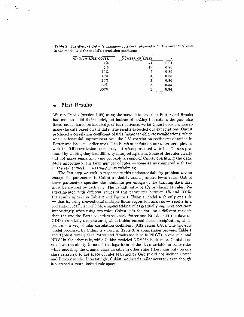
Table 2. The effect of Cubist’s minimum rule cover parameter on the number of rules in the model and the model’s correlation coefficient.

MINIMUM RULE COVER NUMBER OF RULES T

1% 41 0.91 5% 1 2 0.90

10% 7 0.89 15% 4 0.88 20% 3 0.86 25% 2 0.85

100% 1 0.84

4 First Results

We ran Cubist (version 1.09) using the same data sets that Potter and Brooks had used to build their model, but instead of making the cuts in the piecewise linear model based on knowledge of Earth science, we let Cubist decide where to make the cuts based on the data. The results exceeded our expectations. Cubist produced a correlation coefficient of 0.91 (using ten-fold cross-validation) , which was a substantial improvement over the 0.86 correlation coefficient obtained in Potter and Brooks’ earlier work. The Earth scientists on our team were pleased with the 0.91 correlation coefficient, but when presented with the 41 rules produced by Cubist, they had difficulty interpreting them. Some of the rules clearly did not make sense, and were probably a result of Cubist overfitting the data. More importantly, the large number of rules - some 41 as compared with two in the earlier work - was simply overwhelming.

The first step we took in response to this understandability problem was to change the parameters to Cubist so that it would produce fewer rules. One of these parameters specifies the minimum percentage of the training data that must be covered by each rule. The default value of 1% produced 41 rules. We experimented with different values of this parameter between 1% and 100%; the results appear in Table 2 and Figure 1. Using a model with only one rule - that is, using conventional multiple linear regression analysis - results in a correlation coefficient of 0.84, whereas adding rules gradually improves accuracy. Interestingly, when using two rules, Cubist split the data on a different variable than the one the Earth scientists selected. Potter and Brooks split the data on GDD (essentially temperature), while Cubist instead chose precipitation, which produced a very similar correlation coefficient (0.85 versus 0.86). The two-rule model produced by Cubist is shown in Table 3. A comparison between Table 1 and Table 3 reveals that Potter and Brooks modeled ln(NDV1) in one rule, and NDVI in the other rule, while Cubist modeled NDVI in both rules. Cubist does not have the ability to model the logarithm of the class variable in some rules while modeling the original class variable in other rules (there can only be one class variable), so the space of rules searched by Cubist did not include Potter and Brooks’ model. Interestingly, Cubist produced similar accuracy even though it searched a more limited rule space.

0.91

0.:

- 0.8s K a, 0 .- .- - '5 0.88 8 K 0 .- 5 0.87 2

E 0.86

-

0.85

0.84

I I

I

i 0 5 10 15 20 25 30 35 40 45

number of rules

Fig. 1. The number of rules in the Cubist model and the correlation coefficient for several different values of the minimum rule cover parameter.

Table 3. The two rules produced by Cubist when the minimum rule cover parameter is set to 25%.

Rule 1: if

then PPT <= 25.457

NDVI = -3.22 + 7.07 PPT + 0.0521 CDD - 84 AMI + 0 . 4 ln(PPT) + 0.0001 GDD

Rule 2: if

then PPT > 25.457

NDVI = 386.327 + 316 AMI + 0.0294 GDD - 0.99 PPT + 0.2 ln(PPT)

Fig. 2. Map showing which of the two Cubist rules are active across the globe.

In machine learning there is frequently a tradeoff between accuracy and understandability. In this case, we are able to move along the tradeoff curve by adjusting Cubists’ minimum rule cover parameter. Figure 1 illustrates this tradeoff by plotting the number of rules and the correlation coefficient produced by Cu- bist for each value of the minimum rule cover parameter in Table 2. We believe that generally a model with fewer rules is easier to understand, so the figure essentially plots accuracy against understandability. We used trial and error to select values for the minimum rule cover parameter that produced the number of rules we wanted for understandability reasons. Based on this experience, We concluded that a useful feature for future machine learning algorithms would be the ability to directly specify the maximum number of rules in the model as a parameter to the learning algorithm. After reviewing a draft of a conference paper on our NDVI work (Schwabacher and Langley, 2001), Ross Quinlan decided to implement this feature in the next version of Cubist - see Section 7.2.

5 Visualization of Spatial Models

Reducing the number of rules in the model by modifying Cubists’ parameters made the model more understandable, but to further understand the rules, we decided to plot which ones were active where. We developed special-purpose C code, which produced the map in Figure 2. In this figure, the white areas represent portions of the globe that were excluded from the model because they are covered with water or ice, or because there was insufficient ground-based data available. After excluding these areas, we were left with 13,498 points that were covered by the model. The light gray areas are the areas in which Rule 1

Fig. 3. Map showing which of the seven Cubist rules are active across the globe.

from Table 3 applies (the drier areas), and the dark gray areas are the areas in which Rule 2 from Table 3 applies (the wetter areas).

Figure 3 shows where the various rules in a seven-rule model are active. In this figure, the white regions were excluded from the model, as before. The gray areas represent regions in which only one rule applies; the seven shades of gray correspond to the seven rules. (We normally use different colors for the different rules, but resorted to different shades of gray for this book.) The black areas are regions in which more than one rule in the model applied. (In these cases, Cubist uses the average of all applicable rules.) The seven rules corresponding to this map are shown in the Table 4.

The Earth scientists on our team found these maps very interesting, because one can see many of the Earth’s major topographical and climatic features. The maps provide valuable clues as to the scientific significance of each rule. With the aid of this visualization, the scientists were better able to understand the seven-rule model. Before seeing the map, the scientists had difficulty interpreting Rule 7, since its conditions specified that CDD and GDD were both high, which appears to specify that the region is both warm and cold. After seeing the map showing where Rule 7 is active, they determined that Rule 7 applies in the northern boreal forests, which are cold in the winter and fairly warm in the summer. The seven-rule model, which is made understandable by this visualization, is almost as accurate as the incomprehensible 41-rule model (see Table 2). This type of visualization could be used whenever the learning task involves spatial data and the learned model is easily broken up into discrete pieces that are applicable in different places, such as rules in Cubist or leaves in a decision tree.

Table 4. The seven rules for NDVI produced by Cubist when the minimum rule cover parameter is set to 10%.

Rule 1: if CDD <= 16.52 PPT <= 25.457

NDVI = 3.48 + then

Rule 2: if COD > 16.52 PPT <= 25.457

NDVI = -69.99 then

Rule 3: if

7.17 PPT - 161 AMI - 0,0082 GOD - 9.9 ln(PPT) + 0.0003 CDD

+ 16.08 PPT - 0.0449 GDD - 263 AMI + 0.0352 CDD + 0.4 ln(PPT)

AMI <=z -0.09032081 PPT > 25.457

NDVI = 375.9 + 367 AMI + 0.0257 GDD - 0.01 PPT + 0.2 Ln(PPT) then

Rule 4: if GDD C= 1395.62 PPT > 25.457

NDVI = 267.3 + 0.12 GDD + 0.0036 CDD + 3 AMI - 0.01 PPT + 0.2 ln(PPT) then

Rule 5: if AMI > -0.09032081 GDD > 5919.36

NDVI = 601.1 - 0.0063 GOD then

0.11 PPT + 3 AMI + 0.2 ln(PPT) + 0.0001 CDD

Rule 6: if AMI > -0.09032081 CDD <= 908.73 GDD > 1395.62 GDD <= 5919.36

NDVI = 359.8 + 317 AMI + 0.037 GOD + 0.0425 CDD then

1 PPT + 0.2 ln(PPT)

Rule 7: if AMI > -0.09032081 CDD > 908.73 GDD > 1395.62

NDVI = 373.13 + 0.0645 GDD + 249 AMI - 1.32 PPT + 0.0134 CDD + 0.2 ln(PPT) then

I

-. i;

Fig. 4. Map showing the errors of the Cubist prediction of NDVI across the globe.

A second visualization tool that we developed (also as special-purpose C code) shows the error of the Cubist predictions across the globe. In Figure 4, white represents either zero error or insufficient data, black represents the largest error, and shades of gray represent intermediate error levels. From this map, it is possible to see that the Cubist model has large errors in Alaska and Siberia, which is consistent with the belief of the Earth scientists on our team that the quality of the data in the polar regions is poor. Such a map can be used to better understand the types of places in which the model works well and those in which it works poorly. This understanding in turn may suggest ways to improve the model, such as including additional attributes in the training data or using a different learning algorithm. Such a visualization can be used for any learning task that uses spatial data and regression learning.

6 Discovery of Quantitative Errors in the Data

Having successfully trained Cubist using data for one year, we set out to see how well an NDVI model trained on one year’s data would predict NDVI for another year. We thought this exercise would serve two purposes. If we generally found transfers across years, that would be good news for Earth scientists, because it would let them use the model to obtain reasonably accurate NDVI values for years in which satellite-based measurements of NDVI are not available. On the other hand, if the model learned from one year’s data transferred well to some years but not others, that would indicate some change in the world’s ecosystem across those years. Such a finding could lead to clues about temporal phenomena in Earth science such as El Niiios or global warming.

Table 5. Correlation coefficients obtained when cross-validating using one year’s data and when training on one year’s data and testing on the next year’s data, using the original data set and using the corrected data set.

DATA SET CROSS-VALIDATE 1983 CROSS-VALIDATE 1984 CROSS-VALIDATE 1985 CROSS-VALIDATE 1986 CROSS-VALIDATE 1987 CROSS-VALIDATE 1988 TRAIN 1983, TEST 1984 TRAIN 1984, TEST 1985 TRAIN 1985, TEST 1986 TRAIN 1986, TEST 1987 TRAIN 1987, TEST 1988

T , ORIGINAL r , CORRECTED 0.97 0.91 0.97 0.91 0.92 0.92 0.92 0.92 0.91 0.91 0.91 0.91 0.97 0.91 0.80 0.91 0.91 0.91 0.91 0.91 0.90 0.90

What we found, to our surprise, is that the model trained on 1983 data worked very well when tested on the 1984 data, and that the model trained on 1985 data worked very well on data from 1986, 1987, and 1988, but that the model trained on 1984 data performed poorly when tested on 1985 data. The second column of Table 5 shows the tenfold cross-validated correlation coefficients for each year, as well as the correlation coefficients obtained when testing each year’s model on the next year’s data. Clearly, something changed between 1984 and 1985. At first we thought this change might have been caused by the El Niiio that occurred during that period.

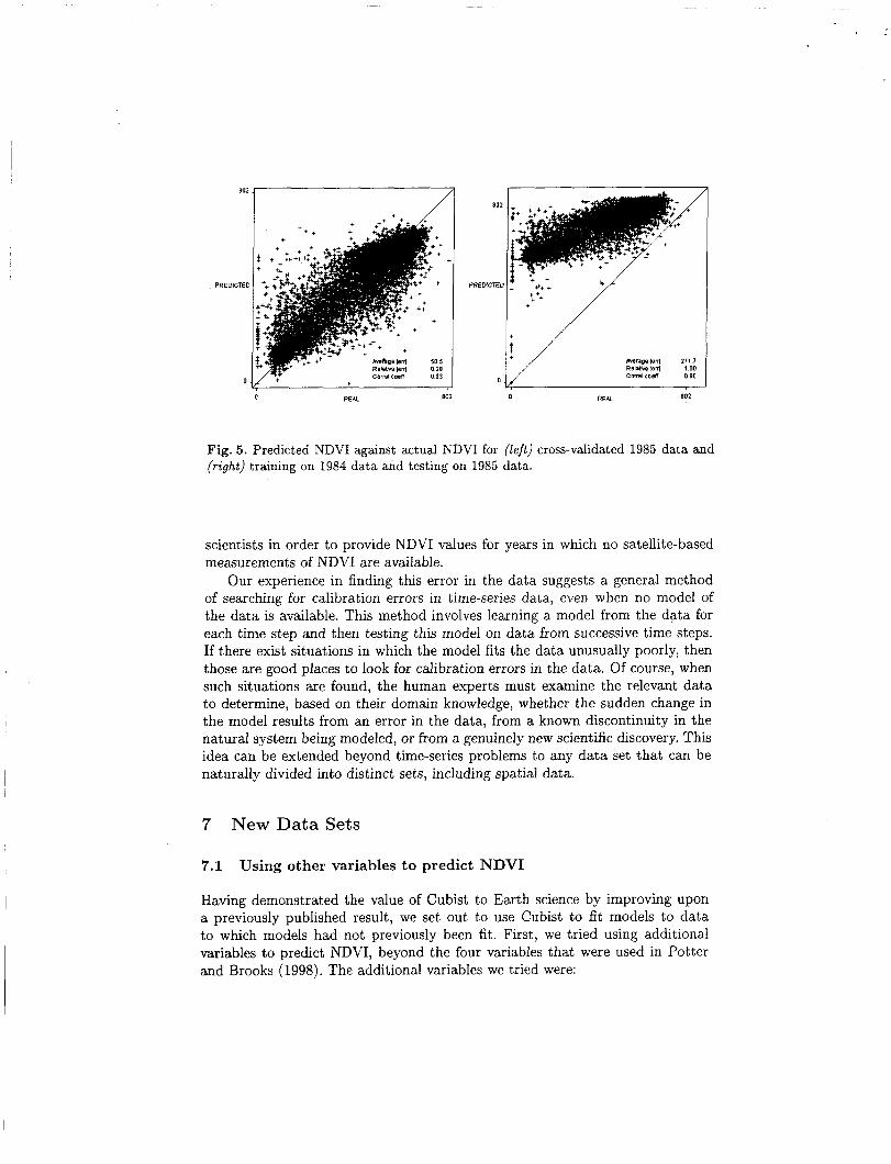
Further light was cast on the nature of the change by examining the scatter plots that Cubist produces. In Figure 5 , the graph on the left plots predicted NDVI against actual NDVI for the 1985 cross-validation run. The points are clustered around the 2 = y line, indicating a good fit. The graph on the right plots predicted against actual NDVI when using 1985 data to test the model learned from 1984 data. In this graph, the points are again clearly clustered around a line, but one that has been shifted away from the 2 = y equation. This shift is so sudden and dramatic that the Earth scientists on our team believed that it could not have been caused by a natural phenomenon, but rather that it must be due to problems with the data.

Further investigation revealed that there was in fact an error in the data. In the data set given to to us, a recalibration that should have been applied to the 1983 and 1984 data had not been done. We obtained a corrected data set and repeated each of the Cubist runs from Table 5, obtaining the results in the third c01umn.~ With the corrected data set, the model from any one year transfers very well to the other years, so these models should be useful to Earth

All of the results presented in the previous sections are based on the corrected data set.

I 0 REAL 802 0 REAL 802

Fig. 5 . Predicted NDVI against actual NDVI for (left) cross-validated 1985 data and (right) training on 1984 data and testing on 1985 data.

scientists in order to provide NDVI values for years in which no satellite-based measurements of NDVI are available.

Our experience in finding this error in the data suggests a general method of searching for calibration errors in time-series data, even when no model of the data is available. This method involves learning a model from the data for each time step and then testing this model on data from successive time steps. If there exist situations in which the model fits the data unusually poorly, then those are good places to look for calibration errors in the data. Of course, when such situations are found, the human experts must examine the relevant data to determine, based on their domain knowledge, whether the sudden change in the model results from an error in the data, from a known discontinuity in the natural system being modeled, or from a genuinely new scientific discovery. This idea can be extended beyond time-series problems to any data set that can be naturally divided into distinct sets, including spatial data.

7 New Data Sets

7.1 Using other variables to predict NDVI

Having demonstrated the value of Cubist to Earth science by improving upon a previously published result, we set out to use Cubist to fit models to data to which models had not previously been fit. First, we tried using additional variables to predict NDVI, beyond the four variables that were used in Potter and Brooks (1998). The additional variables we tried were:

- -

- Potential Evapotranspiration (PET): potential loss of water from the soil both by evaporation and by transpiration from the plants growing thereon. Defined by Thornthwaite (1948).

- Elevation (DEM) - Percentage wetland (WETLND) - HET2SOLU: a 2-dimensional measure of heterogeneity that counts the num-

ber of different combinations of soil and landuse polygons within each grid cell.

- HET3SOLU: a 3-dimensional measure of heterogeneity that takes elevation into account.

- Vegetation type according to the University of Maryland (UMDVEG) - Vegetation type according to the CASA model (CASAVEG)

We found that the variable that produced the largest improvement in accuracy when used together with the original four variables was UMDVEG. In- cluding UMDVEG together with the original four variables increased the cross- validated correlation coefficient (with a minimum rule cover of 1%) from 0.91 to 0.94. Further investigation of this variable, however, revealed that it was derived from NDVI, so that using it to predict NDVI would not be useful.

We found that including PET, DEM, WETLND, and HET2SOLU (along with the original four variables) increased the cross-validated correlation coefficient (using a minimum rule cover of 1%) from 0.91 to 0.93. This model has 40 rules, and is very difficult to understand. Increasing the minimum rule cover parameter to 10% produced a model with seven rules and a cross-validated correlation coefficient 0.90. This model is slightly more accurate than the model produced from the original four variables (which had a cross-validated correlation coefficient of 0.89) and is somewhat harder to understand.

We concluded that the four variables chosen by Potter and Brooks (1998) appear to be a good choice of variables for building a model that is both accurate and understandable. In applications for which accuracy is inore important than understandability, it may be better to use the model with eight variables and 40 rules.

7.2 Predicting NPP

We decided to try using Cubist to predict another measure of vegetation: Net photosynthetic accumulation of carbon by plants, also known as net primary production (NPP). While NDVI is used as an indicator of the type of vegetation at different places, NPP is a measure of the rate of vegetation growth. It is usually reported in grams of carbon per square meter per year.

NPP provides the energy that drives most biotic processes on Earth. The controls over NPP are an issue of central relevance to human society, mainly because of concerns about the extent to which NPP in managed ecosystems can provide adequate food and fiber for an exponentially growing population. In addition, accounting of the long-term storage potential in ecosystems of atmospheric carbon dioxide (CO2) from industrial pollution sources begins with an understanding of major climate controls on NPP.

NPP is measured in two ways. The first method, known as “destructive sampling,” involves harvesting and weighing all of the vegetation in a defined area, and estimating the age of the vegetation using techniques such as counting the number of rings in the cross-sections of trees. The second method uses towers that sample the atmosphere above the vegetation, and estimating NPP from the net COz uptake. Both methods are expensive and provide values for only one point a t at time, so until recently NPP values were only available for a small number of points on the globe.

Previous ecological research has shown that surface temperature and precipitation are the strongest controllers of yearly terrestrial NPP at the global scale (Lieth 1975; Potter et al., 1999). Lieth (1975) used single linear regression to predict NPP from either temperature or precipitation, using a data set containing NPP values from only a handful of sites.

We recently obtained a new, much larger NPP data set from the Ecosystem Model-Data Intercomparison (EMDI) project, sponsored by the National Center for Ecological Analysis and Synthesis (NCEAS) in the U.S. and the International Geosphere Biosphere Program (IGBP). This data set contains NPP values from 3,855 points across the globe. We decided to try using Cubist to predict NPP from the following three variables:

- annual total precipitation in millimeters, 1961-1990 (PPT) - average mean air temperature in degrees centigrade, 1961-1990 (AVGT) - biome type, a discreet variable with 12 possible values (BIOME)

After Ross Quinlan reviewed a draft of a conference paper on our NDVI work (Schwabacher and Langley, 2001), he implemented a new feature in Cubist that allows the user to directly specify the maximum number of rules, rather than having to use trial and error to pick a value of the minimum rule cover parameter that will produce the desired number of rules. For the NPP prediction, we used a new version of Cubist (version 1.10) that includes this new feature. We specified a maximum of five rules. Cubist produced the four rules shown in Table 6, and a cross-validated correlation coefficient of 0.98.

The Earth scientists on our team were very happy with the 0.98 correlation coefficient, and felt that the rules generally made sense. They liked the idea of having different linear models for different groups of biome types. Initially, however, they were surprised that the coefficient on AVGT was negative in three of the four rules. After giving it more thought, they came up with a plausible explanation of why this coefficient is negative. AVGT is acting mainly as a predictor of relatively higher (or lower) heat fluxes that tend to severely dry out (or leave moist) the soils and plants, given a similar PPT. This explanation still requires further investigation.

To help understand these four rules, we produced a map showing where the rules are active. Initially we produced a map with four colors representing the four rules, and black representing multiple rules being active or no rules being active (as in Figure 3). The result was a map in which almost all of the land area was black, which of course was not useful. It turns out that with this set

Table 6. The four rules produced by Cubist for predicting NPP.

Rule 1: if

then PPT <= 653

NPP = 63.8 + 0.49 PPT - 6.5 AVGT Rule 2:

if

then BIOME in {Grassland, Wooded-grassland, Shrubland, ENL-forest-boreal)

NPP = 94.3 + 0.418 PPT - 7.3 AVGT

Rule 3: if

then BIOME in {Forest-temperate, Forest-boreal, Forest-xeric)

NPP = 215.1 + 0.377 PPT - 2.4 AVGT

Rule 4: if BIOME in {Savanna, EBL-forest-tropical, Forest-tropical,

DBL-f orest-tropical) then NPP = 115.4 + 29.1 AVGT + 0.056 PPT

Fig. 6. Map showing which combinations of the four Cubist rules for NPP are active across the globe.

of rules, for much of the land area, two rules are active. Since there are only four rules, and the last three are mutually exclusive, we were able to assign a different color to each of the eight possible combinations of rules. Also, the 3,855 points in our NPP data are from 12 biome types, while approximately 48% of the world’s land area has biome types other than these 12, resulting in no rule being active. Most of these points are tundra, desert, or cultivated land, which are biome types for which NPP has not been measured. We assigned a ninth color to represent these areas. In addition, the global data set and the NPP data set use two different sets of discrete values for biome type. Some of the biome types in the global data set map into more than one biome type in the NPP data set, and in some cases these multiple biome types appear in multiple Cubist rules, making it unclear which Cubist rules are active. These ambiguous points account for approximately 17% of the world’s land area; we assigned a tenth color to these points. The resulting map (translated into shades of gray for this book) is shown in Figure 6. The black areas in this map are the ambiguous points.

The Earth scientists on our team felt that this map was useful in understanding the rules, and in understanding the coverage of the model. It showed them that the current EMDI data set of measured NPP values allows for a somewhat limited extrapolation of the Cubist model (with no deserts, tundra, or cultivated areas), but that the extrapolation still covers a substantial portion of the global land surface, and that it covers most of the naturally “green” areas.

8 Related Work

Robust algorithms for flexible regression have been available for some time. Breiman, Friedman, Olshen, and Stone’s (1984) CART first introduced the no- tion of inducing regression trees to predict numeric attributes. CART trees have a numeric constant at each leaf, yielding a piecewise constant model. Weiss and Indurkhya (1993) extended the idea to rule induction, inducing a set of rules where the right-hand side of each rule has a numeric constant. Quinlan extended the idea to piecewise linear models, by putting a linear model at each leaf of a decision tree in M5 (Quinlan, 1992) or on the right-hand side of each of a set of rules in Cubist (RuleQuest, 2002). Each approach has proved successful in many domains, and both CART and Cubist have achieved commercial suc- cess. However, neither approach has yet seen much application to Earth science data, despite the considerable work on classification learning for tasks like as- signing ground cover types to pixels (e.g., Brodley & Friedl, 1999) and clustering adjacent pixels into groups (e.g., Ester, Kriegel, Sander, & Xu, 1996).

The work on communicability and understandability described in this chapter builds on previous work in comprehensibility. Our requirement for communicability is similar to Michalski’s (1983) “comprehensibility postulate” which states that the results of computer induction should be in a form that is syntactically and semantically similar to that used by humans experts. A collection of papers on comprehensibility can be found in Kodratoff and NQdellec (1995).

Researchers have also carried out extensive work on techniques for visualizing data and learned knowledge. Tufte (1983) did early influential work on the former topic, whereas Keim and Kriegel (1996) review many of the existing approaches. Rheingans and desJardins (2000) describe a technique for using self-organizing maps to display high-dimensional data, predictions, and errors in two dimensions. Within the data-mining community, researchers have developed a variety of methods for the graphical display of learned knowledge (e.g., Brunk, Kelly, & Kohavi, 1996). However, although much of this work employs a spatial metaphor, little has focused on learned spatial knowledge itself.

Applications of machine learning to Earth science data, as in methods for ground cover prediction (e.g., Brodley & Fkiedl, 1999), regularly display classes on maps. Smyth, Ghil, and Ide (1999) plot predictions of a learned mixture model on the globe, but our approach to visualizing areas in which regression rules match, as well as anomalous regions, appears novel.

The European project SPIN! (2002) is seeking to develop a spatial data mining system by combining data mining tools like C4.5 (Quinlan, 1993) with tools for visualizing spatial data like Descartes (Andrienko & Andrienko, 1999). The planned system will let its users visualize geographically-referenced data on maps, and mine the data using the data-mining tools, from a unified user interface. The researchers plan to test the SPIN! system on applications involving seismic and volcano data. The visualization component of the project seems focused on letting users visualize the data, rather than visualizing the knowledge learned through data mining.

There has also been considerable research on using machine-learned knowledge to detect and either ignore or correct errors in training data. Much of this work has focused on removing cases with faulty class labels (e.g., John, 1995; Brodley & Fkiedl, 1999), but some has addressed detecting errors in the values of predictive variables. GritBot, a product of Quinlan’s RuleQuest Research (2002), detects both errors in the class labels and errors in the predictive values by finding what it calls anomalies: items in the training data that are outliers. We ran GritBot on both the NDVI and the NPP data sets, and it found a number of anomalies. For example, it found a point that had the unusual combination of a high maximum NDVI and a low minimum NDVI. All of the anomalies that GritBot finds are single-point anomalies - each anomaly is one item in the training data, which in the applications described in this chapter means that it is a single point on the globe at a single point in time - so GritBot is not capable of finding the type of systematic error that we describe in Section 6 . Naturally, there are established methods for detecting and correcting calibration problems in remote-sensing systems (e.g., Chen, 1997), but these rely on predefined models. Thus, our use of regression rules to detect systematic errors appears novel to both the machine learning and calibration communities.

9 Future Work

Our collaboration is in its early stages, and we still have many research avenues to explore. Our next step in modeling NDVI will incorporate time explicitly by adding the year to the continuous variables used in regression equations, rather than building a separate model for each year. We hope that by examining the resulting multi-year models, we can learn something about climate change over time.

In this chapter, we have assumed that models with fewer rules are more understandable. In future work, we plan to test this assumption by having the Earth scientists on our team examine various sets of rules that Cubist produces for different parameter values and telling us which sets they think are easier to understand. Naturally, we will also ask them to judge the rules’ plausibility and interestingness from the perspective of Earth science.

Another direction for future work is to develop an extension to the Cubist algorithm that would allow it to take advantage of background knowledge. One possible form of background knowledge would be knowledge of the sign of the coefficients on some of the variables within the linear models. For example, we believe that the coefficient on PPT in the NPP model should always be positive. Pazzani and Bay (1999) describe an algorithm that uses knowledge of the signs of the coefficients to constrain the construction of regression equations. Their algorithm accepts input about the sign of each term, then use an optimization method to find the best weights given the constraints. The resulting equations were just as accurate as the unconstrained linear models on separate test sets, and domain experts found them more comprehensible. It would be interesting to combine Pazzani and Bay’s algorithm with the Cubist algorithm to produce decision rules with linear models that obey sign constraints.

The NDVI predictive model is only one piece of a larger framework, known as CASA (Potter & Klooster, 1998), that Potter’s team has developed to model the Earth’s ecosystem. CASA takes the form of a process model, stated in terms of differential equations, for the production and absorption of biogenic trace gases in the Earth’s atmosphere. CASA’s output is NPP. We have achieved very good accuracy by using Cubist to predict NPP, but for the reasons of understandability and communicability described earlier, we would like our learned models to take the same form as the CASA model, which means we cannot rely on Cubist alone in our future efforts.

There has been some research on discovering laws that take the form of differential equations (Todorovski & Dzeroski, 1997), but this work has not used an existing set of equations as the starting point. We plan to develop an algorithm that will begin with the current CASA model and search through the space of possible equations to find an improved model. We will consider developing a Cubist-like algorithm that learns a model with a set of rules to select among different sets of differential equations (instead of different linear models). We hope that this effort will improve the accuracy of the CASA model to the point where it is as accurate as the Cubist model of NPP, while retaining CASA’s

. .

communicability and its scientific plausibility. We also hope that the changes our system makes to the model will suggest new insights about Earth science.

10 Lessons Learned

In their editorial on applied research in machine learning, Provost and Kohavi (1998) claimed that a good application paper will “focus research on important unsolved problems that currently restrict the practical applicability of machine learning methods.” In this chapter, we have identified, and provided initial so- lutions for, three such problems that arise in scientific applications:

Communicability. In scientific domains, it is important for the form of the learned models to match the form that is customarily used in the relevant literature, so that the learned models can be communicated to other scientists.

Understandability. In domains that involve spatial data, understanding of the models can be increased by visualizing the spatial distribution of the model’s errors and visualizing the locations in which the model’s components (e.g., rules) are active. Adjusting the parameters to the learning algorithm in order to produce a smaller model can also aid understandability.

Quantitative errors. In applications that involve time-series numerical data, machine learning methods can be used to identify quantitative errors by testing a learned model for one time period against data from other time periods.

Although we have developed these ideas in the context of a specific scientific application - the prediction of NDVI and NPP from climate variables - we believe they have general applicability to any domain that involves scientific understanding of spatio-temporal data. As we continue utilizing machine learning to improve the CASA model, we expect that the challenging nature of the task will reveal other methods and principles that contribute to both Earth science and the science of machine learning.

Acknowledgments

We would like to thank Vanessa Brooks for her help in creating the data files. We would also like to thank Jeff Shrager for his help in formulating the problem, and for numerous discussions in which he has participated. Finally, we would like to thank Kazumi Saito and Ross Quinlan for reviewing drafts of this paper. This research was funded by the NASA Intelligent Systems Program.

References

Andrienko, G. L., & Andrienko, N. V. (1999). Interactive maps for visual data exploration. International Journal Geographic Information Science, 13, 355- 374.

.

Breiman, L., Friedman, J . H., Olshen, R. A., & Stone, C. J. (1984). Classification and regression trees. Belmont, CA: Wadsworth.

Brodley, C. E., & Friedl, M. A. (1999). Identifying mislabeled training data. Journal of Artificial Intelligence Research, 11, 131-167.

Brunk, C., Kelly, J., & Kohavi, R. (1996). MineSet: An integrated system for data mining. Proceedings of the Second International Conference of Knowledge Discovery and Data Mining (pp. 135-138). Portland: AAAI Press.

Chen, H. S. (1997). Remote sensing calibration systems: An introduction. Hamp- ton, VA: A. Deepak Publishing.

Ester, M., Kriegel, H.-P., Sander, J.;& Xu, X. (1996). A density-based algorithm for discovering clusters in large spatial databases with noise. Proceedings of the Second International Conference of Knowledge Discovery and Data Mining (pp. 226-231). Portland: AAAI Press.

John, G. A. (1995). Robust decision trees: Removing outliers from data. Proceed- ings of the First International Conference of Knowledge Discovery and Data Mining (pp. 174-179). Montreal: AAAI Press.

Keim, D. A., & Kriegel, H.-P. (1996). Visualization techniques for mining large databases: A comparison. Transactions on Knowledge and Data Engineering,

Kodratoff, Y. & Nedellec, C. (Eds.) (1995). Working Notes of the IJCAI-95 Workshop on Machine Learning and Comprehensibility. Montreal, Canada.

Lieth, H. (1975). Modeling the primary productivity of the world. Pages 237-263 in H. Lieth and R. H. Whittaker, eds., Primary Productivity of the Biosphere. Springer-Verlag, Berlin.

Michalski, R. S. (1983). A theory and methodology of inductive learning. Arti- ficial Intelligence, 20, 111-161.

Pazzani, M. J., & Bay, S. D. (1999). The independent sign bias: gaining in- sight from multiple linear regression. Proceeding of the Twenty-First Annual Meeting of the Cognitive Science Society.

Potter, C. S., & Brooks, V. (1998). Global analysis of empirical relations between annual climate and seasonality of NDVI. International Journal of Remote Sensing, 19, 2921-2948.

Potter, C. S., & Klooster, S. A. (1998). Interannual variability in soil trace gas (CO2, NzO, N O ) fluxes and analysis of controllers on regional to global scales. Global Biochemical Cycles, 12, 621-635.

Potter, C. S., Klooster, S. A., & Brooks, V. (1999). Interannual variability in terrestrial net primary production: Exploration of trends and controls on regional to global scales. Ecosystems, 2(1): 36-48.

Provost, F., & Kohavi, R. (1998). On applied research in machine learning. Machine Learning, 30, 127-132.

Quinlan, J. R. (1992). Learning with continuous classes. Proceedings of the Aus- tralian Joint Conference on Artificial Intelligence (pp. 343-348). Singapore: World Scientific.

Quinlan, J. R. (1993). (74.5: Programs for Machine Learning. San Mateo, CA: Morgan Kaufmann.

8, 923-938.

Rheingans, P., & desJardins, M. (2000). Visualizing high-dimensional predictive model quality. Proceedings of the 1 lth IEEE Visualization Conference. Los Alamitos, CA: IEEE Computer Society.

RuleQuest (2002). RuleQuest Research data mining tools. ht tp: / / www .rulequest. com.

Schwabacher, M., & Langley, P. (2001). Discovering communicable scientific knowledge from spatio-temporal data. Proceedings of the Eighteenth Interna- tional Conference on Machine Learning (pp. 489-496). San Francisco: Morgan Kaufmann.

Smyth, P., Ghil, M., & Ide, K. (1999). Multiple regimes in Northern hemisphere height fields via mixture model clustering. Journal of the Atmospheric Sci- ences, 56.

SPIN! (2002). Spatial mining for data of public interest. ht tp: / / www . ccg .leeds .ac. uk/spin.

Thornthwaite, C. W. (1948). An approach toward rational classification of climate. Geographical Review, 38, 55-94.

Todorovski, L., & Dzeroski, S. (1997). Declarative bias in equation discovery. Proceedings of the Fourteenth International Conference on Machine Learning (pp. 376-384). San Francisco: Morgan Kaufmann.

Tufte, E. R. (1983). The visual display of quantitative information. Cheshire, CT: Graphics Press.

Weiss, S., & Indurkhya, N. (1993). Rule-based regression. Proceedings of the Thirteenth International Joint Conference on Artificial Intelligence (pp. 1072- 1078). Chambery, France.

Willmott, C. J., & Feddema, J. J. (1992). A more rational climate moisture index. Professional Geographer, 4 4 , 84-87.

discovering communicable models from earth science … · discovering communicable models from...

Documents