Earth Mover’s Prototypes: a Convex Learning Approachfor Discovering Activity Patterns in Dynamic Scenes

Gloria ZenDISI, University of Trento

via Sommarive 14, Povo, Italygloria.zen@disi.unitn.it

Elisa RicciFondazione Bruno Kessler

via Sommarive 18, Povo, Italyeliricci@fbk.eu

Abstract

We present a novel approach for automatically discov-ering spatio-temporal patterns in complex dynamic scenes.Similarly to recent non-object centric methods, we use lowlevel visual cues to detect atomic activities and then con-struct clip histograms. Differently from previous works, weformulate the task of discovering high level activity pat-terns as a prototype learning problem where the correla-tion among atomic activities is explicitly taken into accountwhen grouping clip histograms. Interestingly at the core ofour approach there is a convex optimization problem whichallows us to efficiently extract patterns at multiple levels ofdetail. The effectiveness of our method is demonstrated onpublicly available datasets.

1. Introduction

Complex and crowded scenes depicting public spaces(e.g. city roads, subway stations) are especially challeng-ing for video surveillance systems based on the traditionaldetection/tracking paradigm. This is mainly due to the pres-ence of frequent occlusions in the scene and to the lack ofappropriate models taking into account the spatial and tem-poral correlations between multiple objects. To face thesedifficulties, in the last few years there has been a growinginterest in developing non-object centric methods for dy-namic scene understanding [3, 12, 4, 13, 14].

Following this trend, we propose a novel approach forextracting spatio-temporal patterns in complex scenes. Asin previous works [3, 4, 14], we use simple features com-puted from moving foreground pixels to locate atomicevents and we cluster them into atomic activities. Then,given a video stream we divide it into short clips and foreach clip we compute a histogram by summing up the oc-currences of atomic activities. Previous works [3, 4, 14]adopting this ‘word-document’ representation assume thatwords do not follow a specific order into documents, thus

ignoring that atomic activities are not independent. Thisimplies an information loss since it is not possible to dis-tinguish among groups of atomic activities correspondingto similar motion patterns (e.g. cars moving in the same di-rection in the same lane) and those representing objects ofdifferent size/speed in faraway regions of the scene.

In this paper, we propose to overcome this drawbackby taking into account the similarity between atomic activ-ities whilst learning the underlying behavioral patterns ofthe scene. We present a novel algorithm which adopts theEarth Mover’s Distance (EMD) [9] in the objective func-tion of the learning problem and outputs a set of histogramsprototypes representing the discovered patterns. The maincontributions of this paper are the following:

1. We formulate the task of mining typical behaviors indynamic scenes as a prototype learning problem. Our ap-proach is based on a convex optimization problem, specif-ically a Linear Program (LP), thus, it is not prone to localminima, it is rather scalable and it is easy to implement. Torun experiments on medium-large scale datasets, followingthe idea in [7], we also develop a variant of our algorithmdrastically reducing its computational cost.

2. We show how, with the proposed approach, salientpatterns at multiple scales can be discovered. Differentlyfrom previous works and thanks to the theory of Paramet-ric LP [1, 8], our algorithm performs a multiscale temporalsegmentation of the video scene in one shot.

3. Comparing salient aspects extracted at multiple scalescan also be useful in individuating anomalous patterns. Tothis aim we propose a Multiscale Anomaly Score (MAS).

We evaluate extensively our approach on four datasets(three of which are publicly available), showing that it of-fers competitive performance w.r.t. state-of-the-art meth-ods. To our knowledge few resources (annotated video se-quences, source codes) are publicly available for complexscenes analysis. To help filling this gap our code and theresults from our experiments are made available to the com-munity (http://disi.unitn.it/∼zen).

Related Works. Among previous works on complex

3225

Our [6] [3] [14] [4] [12]atom. activities correlation

√× × × × ×

multiscale analysis√

× ×√

× ×convexity

√× × × × ×

learning temporal rules × ∠√

×√ √

anomaly detection√ √ √

×√ √

Table 1. Qualitative comparison of the proposed and previousworks: (

√=yes, ×=no, ∠=partially).

scene analysis, those based on Probabilistic Topic Mod-els (PTMs) [3, 12, 4, 6] have shown great potential. Re-cent works on hierarchical PTMs [3, 4] focus mainly onmodeling the behaviors’correlation over time and inferringglobal rules. In this paper, we address different aspects try-ing to overcome some drawbacks of PTMs. First, we gobeyond the usual word-document paradigm by taking intoaccount the similarities among words during learning. Sec-ond, as our learning algorithm is based on a LP problem,we avoid the risk of being stacked into bad local minimatypical of EM-like procedures. Third, by parametric LP,spatio-temporal activity patterns at multiple scales can bediscovered efficiently and, under special conditions, with-out retraining from scratch. Another work similar to oursis [14], where a multiscale scene analysis is performed us-ing diffusion maps in a preprocessing step before cluster-ing. Differently, our multi-resolution analysis takes place inthe clustering phase and it is also used for individuating un-usual behaviors. Table 1 resumes the main features of ourapproach compared to previous works.

2. Preliminaries

LP and Parametric LP. Given A ∈ IRn×m, c,a ∈IRm, b ∈ IRn, a LP in standard form [1, 8] is:

minx≥0 c′x s.t. Ax = b

If the matrix A is of full rank and the polyhedron D = x :Ax = b,x ≥ 0 is bounded and non-empty, the LP hasa bounded optimal solution. Let B ∈ I = 1, ...,m bean ordered set of n column indexes. Let AB be the n × nsub-matrix of A whose i-th column is Ai. The set B iscalled a feasible basis if AB is of full-rank and A−1

B b ≥ 0.A column Ai, i ∈ B is called a basic column, otherwiseit is a non-basic column and belongs to the set N = I −B. A basic feasible solution (bfs) x associated to a feasiblebasis B is obtained by xB = A−1

B b and xN = 0. A bfsis optimal if it corresponds to a solution of the LP. Thereis a bijection between bfs and vertices of D. The simplexmethod systematically explores the extreme points (bfs) ofD starting from an initial extreme, until an optimal one isfound. Given λ ∈ R a parametric LP has the form:

minx≥0

(c + λa)′x s.t. Ax = b (1)

Earth Mover’s Distance. When comparing histograms,standard bin-to-bin distance functions (e.g. Lp distances, KLdivergence) assume that the domains of the histograms arealigned, an assumption that is often violated due to noise.On the contrary EMD [9] addresses the alignment problembeing a cross-bin distance function. The EMD(h,k) be-tween two histograms h and k is obtained as the solution ofthe transportation problem:

minfqt≥0

D∑q,t=1

dqtfqt s.t.D∑q=1

fqt = ht,

D∑t=1

fqt = kq (2)

provided that the histograms are normalized to unit mass,i.e.∑q k

q = 1 and∑t h

t = 1. The variable fqt denotesa flow representing the amount transported from the q-thsupply to the t-th demand and dqt the ground distance.

3. Discovering Patterns in Complex Scenes3.1. Overview

In this Subsection we describe the proposed approachfor discovering spatio-temporal patterns in dynamic scenes.Fig. 1 illustrates the main steps of our method.

In the first phase low level features are extracted fromthe video and are used to define atomic events. We first ap-ply a background subtraction algorithm to extract pixels offoreground. We found a simple dynamic Gaussian-Mixturebackground model [11] sufficient in our scenarios. We alsocompute the optical flow vector using the Lucas-Kanade al-gorithm. By thresholding the magnitude of the optical flowvectors we classify foreground pixels into static and movingpixels. We further differentiate among moving pixels quan-tizing the optical flow into 8 directions. Then we dividethe scene into p × q patches. For each patch we considerthe foreground pixels and their optical flow vectors and webuild a patch descriptor vector v = [x y fg dof mof ] where(x, y) denotes the coordinates of the patch center in the im-age plane, fg represents the percentage of foreground pixelsin the patch and dof and mof are respectively the mode ofthe orientations distribution and the average magnitude ofoptical flow vectors in the patch. For patches of static pix-els we set dof = mof = 0. We define an atomic event asa patch descriptor v such that fg ≥ Tfg , i.e. we excludepatches with few pixels of foreground.

In the second phase we group atomic events with K-medoids clustering, rather than with K-means due to itsincreased robustness to noise and outliers. Each cluster rep-resents an atomic activity. Then, we divide the video intoshort clips and for each clip we construct an activity his-togram hc representing the distribution of atomic activitiesin the c-th clip. Finally, the clips are grouped according totheir similarity. To this aim we propose a novel algorithmwhich given a set of clips histograms identifies a smallerset of histogram prototypes representing the salient activi-

3226

Figure 1. Flowchart of the proposed approach (best viewed in color)

ties occurring in the scene. In the following we describe theprototype learning algorithm.

3.2. Convex Prototype Learning

Suppose a set of histograms H = h1, . . . ,hN, hi∈ IRD is given. We aim to learn N representative proto-types P = p1, . . . ,pN, pi ∈ IRD, each one associatedto the original hi, such that their similarity with respectto the original data is maximized. Moreover, we want theset of prototypes to be a sparse representation of the origi-nal dataset H, i.e. the number of different prototypes to besmall. This can be obtained by minimizing their reciprocaldifferences. The overall task can be formalized as follows:

minpi∈Ω

N∑i=1

L(hi,pi) + λ∑i 6=j

ηijJ (pi,pj) (3)

The feasible region Ω = p : ∀t pt ≥ 0,∑t pt = 1 is

meant to ensure that the prototypes are histograms normal-ized to unit mass. The objective function consists of twoterms. The first term or loss should penalize the differencebetween the given histograms and the associated prototypes.The second term or regularization term must enforce thesmoothness among related prototypes. Their relative im-portance is controlled by the positive coefficient λ. Whenλ = 0 all prototypes pi must be equal to their correspond-ing histograms hi while for λ → ∞ all prototypes shouldbe equal to each others. For 0 ≤ λ < ∞ a number ofdifferent prototypes between N and 1 can be obtained.

Learning Prototypes with EMD. In this paper we focusour attention on the cases where L(·) and J (·) are convexfunctions and specifically we present a formulation of (3)where the EMD is adopted as loss function:

minpi∈Ω

N∑i=1

EMD(hi,pi) + λ∑i 6=j

ηij maxq=1...D

|pqi − pqj | (4)

The advantage of using EMD is motivated by the fact thatthe ground distances dqt can encode information about thesimilarity of atomic activities. To this aim, since eachatomic activity q is represented by the associated exemplarmq computed by K-medoids, we set dqt = ‖mq −mt‖2.

As stated above the rightmost term in (4) is meant tominimize the number of different prototypes. The adop-tion of the L1 norm induces sparsity, thus producing a smallnumber of prototypes. Generally a comparison among all

possible pairs pi,pj , i 6= j, is required imposing all pro-totypes to be close to each other. However this implies anincreased computational cost when solving (4). To alleviatethis fact we introduce the binary coefficients ηij ∈ 0, 1in order to select only a subset of pairs of histograms whichmust be merged. In the absence of prior knowledge, wecan simply identify for each histogram hi a set of P nearestneighbors and set ηij = 1 if hj is a neighbor of hi. Al-ternatively, temporal dependencies can be encoded: if his-tograms represent temporally adjacent clips we set ηij = 1if i = j − 1,∀j = 2 . . . N , ηij = 0 otherwise. As shown inthe experimental section, we tested both approaches: in thefollowing we refer to them respectively as nearest neigh-bors clustering and temporal segmentation. Note that thecoefficients ηij are fixed and do not change during learning.To compute histogram prototypes we substitute the EMDdefinition (2) in the loss in (4) we get the following LP:

minpqi ,fiqt,ζij≥0

N∑i=1

D∑q,t=1

dqtfiqt + λ

∑i 6=j

ηijζij (5)

s.t. −ζij ≤ pqi − pqj ≤ ζij , ∀q,∀i, j

D∑q=1

f iqt = hti, ∀tD∑t=1

f iqt = pqi , ∀q,∀i

where we introduced the slack variables ζij . Note that theconstraints

∑t pti = 1 are removed since they are automati-

cally satisfied. It is worth noting that at the coordinate levelwe adopt the L∞ norm rather than the L1 norm. This doesnot promote sparsity but it produces the effects that all co-ordinates of a prototype go to zero together and it reducessignificantly the computational cost of solving (5), limitingthe number of slack variables.

Learning Prototypes with EMD-L1. For large N andD solving (5) is still time consuming even for today’s so-phisticated LP solvers. The computational cost is espe-cially high due to the large number of flow variables f iqt.Actually, we do not specifically need them since we areonly interested in computing the prototypes pi. To speedup calculations we propose a modification of (5) whichadopts EMD with L1 distance over bins as ground distance,i.e. dqt = |q − t|. The idea is that similar atomic activi-ties should correspond to neighboring bins in activities his-tograms. To this aim we sort the cluster medoids computedwith K-medoid according to the associated motion informa-tion from exemplars corresponding to static events to those

3227

associated with optical flows with large magnitude. The ori-entation is also taken into account in this phase.

In case of EMD-L1 every positive flow between farawayhistogram bins can be replaced by a sequence of flows be-tween neighbor bins [7]. Thus (2) can be simplified as:

mingq,q+1,gq,q−1≥0

D−1∑q=1

gq,q+1 +

D∑q=2

gq,q−1 (6)

s.t. gq,q+1 − gq+1,q + gq,q−1 − gq−1,q = hq − pq ∀q

With (6) the number of variables and constraints decreasessignificantly. In particular the number of flow variables in-volved reduces from O(D2) to O(D). This is greatly ben-eficial in terms of computational cost since the number ofvariables is a dominant factor in the time complexity of allLP algorithms. With these premises, we simplify (5) bysubstituting the EMD-L1 definition (6) in the loss:

min

N∑i=1

D−1∑q=1

giq,q+1 +

N∑i=1

D∑q=2

giq,q−1 + λ∑i 6=j

ηijζij (7)

s.t. −ζij ≤ pqi − pqj ≤ ζij , ∀q, ∀i, j, i 6= j

giq,q+1 − giq+1,q + giq,q−1 − giq−1,q = hqi − pqi , ∀q, i

pqi , giq,q+1, g

iq,q−1, ζij ≥ 0

The resulting optimization problem is a LP with nvar =2N(D − 1) + ND + 1

2N(N − 1) variables if we imposeeach prototype to be close to each other, i.e. ηij = 1 ∀i 6= j.In this case for large datasets (N D) the computationalcost of (7) is dominated by the number of slack variablesthat is quadratic w.r.t. the number of datapoints. However,as we discussed above, by setting some of the ηij = 0, (7)can be solved efficiently even in case of large datasets.

Learning Prototypes with Bin-to-bin Distances. Todemonstrate the advantages of considering cross-bin dis-tances when learning prototypes, we briefly discuss theform that (3) assumes when bin-to-bin distances are consid-ered as loss functions. When L(·) is the square loss, J (·)is a sum of L1 norms and ηij = 1 if i = j − 1 and ηij = 0otherwise, we get something very close to the “total varia-tion denoising” [10] or to the fused lasso1 [2]. When the L1

norm is chosen as loss and a combination of L1-L∞ normsis used for J (·), (3) assumes the form of the following LP:

minpi∈Ω

N∑i=1

D∑q=1

|hqi − pqi |+ λ

∑i 6=j

ηij maxq=1...D

|pqi − pqj | (8)

In the experimental section we show that bin-to-bin dis-tances are less effective than EMD when learning proto-types for dynamic scene understanding.

1Note also that in the fused lasso formulation [2] the feasible region isslightly different from Ω since the pi are not specifically constrained to benormalized histograms.

Algorithm 1 One shot temporal segmentation1: Input: H = (h′1 . . .h

′N )′, i = 0, Ip = ND2 + N + k :

k = 0, . . . , ND.2: Set (5) in standard form (1) according to Proposition 1.3: Find an optimal bfs B0 for λ0 =∞.4: while λi ≥ 05: Compute xi, with xi

Bi = A−1Bi b and xi

Ni= 0.

6: cj = cj − cBiA−1Bi Aj with j ∈ Ni.

7: aj = aj − aBiA−1Bi Aj with j ∈ Ni.

8: m = arg maxj−cj/aj : aj > 0 (entry index)9: λi+1 = −cm/am

10: u = A−1Bi Am.

11: if the support I(u) is empty then return12: ` = arglexico-mintAi

t/ut : t ∈ I(u) (exit index)13: Update Bi+1 = Bi ∪ m\`14: Set Pi = xi

Ip15: i← i+ 116: end17: Output: The set P1, ...PN

3.3. Multiscale Analysis and MAS

A crucial property of (5) and (7) is that the sparsityachieved is controlled by a single parameter, i.e. the reg-ularization constant λ. For λ varying between ∞ and 0 adifferent number of prototypes M(λ) between 1 and N isobtained. Instead of trying to find the value of λ which pro-vides the best prototype representation we propose to ex-ploit the solutions of (5) and (7) for different values of λ.This corresponds to discover different salient activities atmultiple scales. For example, in case of temporal segmen-tation in a traffic scene, for large values of λ we can obtaintwo prototypes, corresponding to a rough description of thescene, distinguishing among clips with moving vehicles andwith vehicles stopped at the traffic lights. As λ decreases wegradually enhance the level of detail differentiating amongvehicles flows of different intensity.

Comparing clustering results at multiple scales we candetect unusual behaviors corresponding to atypical his-tograms. To this aim we define for each hk an associatedanomaly score. The idea is to monitor how the clusters sizechanges for decreasing values of λ. From λ = ∞ (whereall the histograms are represented by a single prototype) toλ = 0 (where each hk corresponds to a different pk), theanomaly score of hk is computed as the sum of the ratiosof the clusters size containing hk at two subsequent scales.Formally we first introduce the notion of sets of fused his-tograms as they are generated by our algorithms.

Definition 1. (Sets of Fused Histograms) Let λ be afixed value λ and Hλk be a set of histograms with k =

1, . . . ,M(λ). Then a valid set of fused histograms Hλk sat-isfies the following properties: the collection of the setsHλk is a partition of H

3228

∀ h`,hm ∈ Hλk we have pq` = pqm ∀ q = 1 . . . D

∀ h` ∈ Hλk and hm ∈ Hλm ∃q : pq` 6= pqmIn a nutshell a set of fused histograms corresponds to his-

tograms associated to the same prototype. Different sets offused histograms are generated for different λ. By lookingat the sets of fused histograms we can define the MAS.

Definition 2. (MAS) Let hk ∈ Hλi

k , hk ∈ Hλi−1

k′ withλi−1 > λi.We define the Multiscale Anomaly Score of hk:

MAS = 1− 1

NL

L∑i=1

|Hλi−1

k′ ||Hλi

k |(9)

Thus analyzing multiple scales we can distinguish betweencases where a cluster with a single histogram is merged athigher level with a small cluster and situations where it be-longs to a big cluster: in the first case its MAS is higher.Note that MAS definition is possible since with our ap-proach if two histograms belong to the same fused set forλ = λ they will generally remain fused for any λ ≥ λ. Asa final remark we should say that while large values of Lusually result in more accurate estimates of MAS, this alsoincreases the computational cost since (5) must be solvedL times. In the following we show how in some cases allpossible sets of fused histograms can be obtained with com-putational cost comparable with that of solving (5) once.

3.4. Multiscale Analysis in One Shot

In this section we focus our attention on EMD prototypelearning, and we show that since (5) is a parametric LP analgorithm based on a variant of the revised simplex method[8] can be used to compute all possible sets of prototypesfor increasing values of λ. We consider the specific case oftemporal segmentation i.e. we set ηij = 1 for i = j−1, j =2 . . . N and ηij = 0 otherwise.

Let H′ = (h′1 . . .h′N ), P′ = (p′1 . . .p

′N ), H,P ∈ IRND.

Let 1 ∈ IRD denote the vector 1 = (1 . . . 1), I be the iden-tity matrix and 0 be the zero matrix of appropriate dimen-sion. We first define the following block diagonal matricesD ∈ IR(N−1)D×(N−1), D = diag(1), F,G ∈ IRND×ND2

,F = diag(Q),G = diag(T),Q ∈ IRD×D2

, Q = diag(1′),the block Toeplitz matrix Σ ∈ IR(N−1)D×ND, and the ma-trix T ∈ IRD×D2

such that:

Σ =

I -I 0 . . . 00 I -I . . . 0...

. . ....

0 0 . . . I -I

, T =

E1

E2

...ED

,

where I, 0 and −I ∈ IRD×D and Ei = (e′i e′i . . . e′i), e′i ∈IRD, e′i = (0 . . . 0 1 0 . . . 0) with a 1 in the i-th position.

Proposition 1. Let f ∈ IRND2

be the vector of flowvariables, δ+, δ− ∈ IRND, ζ ∈ IRN−1 be slack vari-ables. Let ω ∈ IRND

2

be the vector containing the

ground distance values i.e. ω = (d . . . d), d ∈ IRD2

,d = (d11, . . . d1D d21 . . . dDD). The following elements:x′ =

(f ′ ζ′ P′ δ+

′ δ−′), a′ =

(ω′ 0′ 0′ 0′ 0′

), c′ =(

0′ 1′ 0′ 0′ 0′),

A =

0 -D Σ I 00 -D -Σ 0 IF 0 0 0 0G 0 -I 0 0

, b =

00H0

define (5) in the standard form (1) of a parametric LP.

In [15] Yao and Lee showed that many algorithms in ma-chine learning and specifically the family of regularizationproblems with piecewise linear loss and L1 penalties (suchasL1 SVM) can be written in the form of (1) and the tableausimplex method can be used for solving (1) for all possi-ble values of λ simultaneously. In this paper we proposeto solve (5) using a variation of the algorithm proposed in[15] by considering rather than the tableau simplex method,the revised simplex with the lexico-min rule since it offerscomputational advantages for sparse LPs and avoid situa-tions of degeneracy. The resulting algorithm is presented inAlgorithm 1. The main difficulty when applying Algorithm1 is how to individuate an optimal bfs B0. An optimal bfsB0 can be obtained using any feasible basic index set B0

and running the standard simplex algorithm for the associ-ated LP problem i.e. for a = 0. The following propositionshows an example of a bfs B0 for (5).

Proposition 2. The set of indices B0 = I1 ∪ I2 withI1 = kD+1 : k = 0, . . . , ND−1, I2 = ND2+N+k :k = 0, . . . , 3ND − 2D − 1 individuates a bfs for (5).Similar results can be obtained for (7) and (8) in case oftemporal segmentation. When the coefficients ηij assumearbitrary values, (5), (7) and (8) are also parametric LPproblems and Algorithm 1 can be used for computing theentire solution path. However, in this cases (e.g. for nearestneighbor clustering) determining a suitable bfs B0 is morecomplex and we leave it to further works.

4. Experimental resultsWe tested our method on four datasets. Due to lack of

space we encourage the reader to look at the supplemen-tary material submitted with this paper to see the videosassociated to our results. The proposed approach is fullyimplemented in C++ using the publicly available librariesOpenCV and GLPK 4.2.1 (GNU Linear Programming Kit).

The first dataset consists of a traffic scene sequence de-picting a crossroads. In this scenario different events occurat regular periods as the vehicles flow is controlled by trafficlights. The second dataset is publicly available and is takenfrom APIDIS2. Here players involved in a basketball match

2http://www.apidis.org/Dataset/

3229

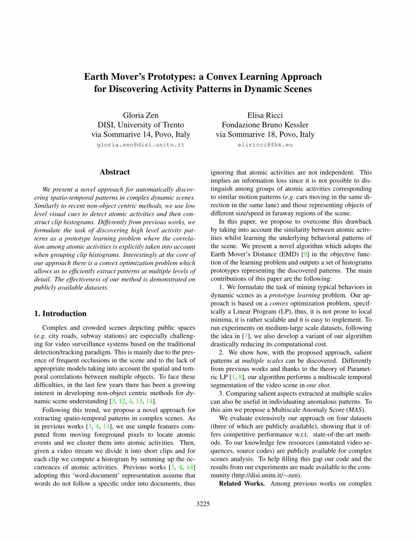
Traffic Basket Junction Roundaboutno frames 6000 6000 90000 93500fps 12 23 25 25no clips 300 100 240 311frame size 276×336 320×368 288×360 288×360patch size 23×21 16×16 12×12 12×12D 8 16 16 16

Table 2. Details of the setting used in our experiments.

(a) (b)Figure 2. Traffic dataset: (a) K-medoids results (b) Example ofatomic activities.

are depicted. In detail we pick the sequence of camera 5from 20080409T184900 to 20080409T185400. The imagesare resized and cropped in a way to include only the basket-ball court. The third and forth datasets [3] are also publiclyavailable3,4. They depict two complex traffic scenes in Lon-don (Junction and Roundabout) and they both correspondto a video of about 1 hour duration. More details about thedatasets and the experimental setup are reported in Table 2.We chose the first dataset since it is suitable for testing ourtemporal segmentation approach, as it corresponds to fewcycles of the traffic lights status and it contains some inter-esting anomalous events. The nearest neighbor clustering isadopted for experiments on the other datasets.

Traffic dataset. We report some results from the firstphase of our analysis, which aims to classify the atomicevents according to their position and motion. Labeledatomic events as they are obtained with K-medoids are de-picted in Fig.2.a, where each color corresponds to a specificatomic activity (note that for visualization purposes we plotonly a small subset of collected events and we add a smallrandom shift to their position (x, y) in the image plane).It is easy to observe that neighboring events belong to thesame group and where the same region contains two clus-ters, the clusters correspond to activities with different mo-tions. Fig.2.b shows this situation: the orange activity cor-responds to vehicles stopped due to red traffic light, whilethe white one shows moving vehicles in the same area whenthe traffic lights are on green.

We further show the effectiveness of our approach insegmenting scene activities in time. Figure 4 shows theresults on 100 clips that we obtained by solving (7) withλ = 5. From each of the 10 clusters obtained we extractone frame, representative for the salient activities (due tolack of space we just show 9 of them). The orange, yellow,and red clusters correspond to the activity of parallel vehi-cle flows (green traffic light), while the light blue, white and

3http://www.eecs.qmul.ac.uk/ jianli/Junction.html4http://www.eecs.qmul.ac.uk/ jianli/Roundabout.html

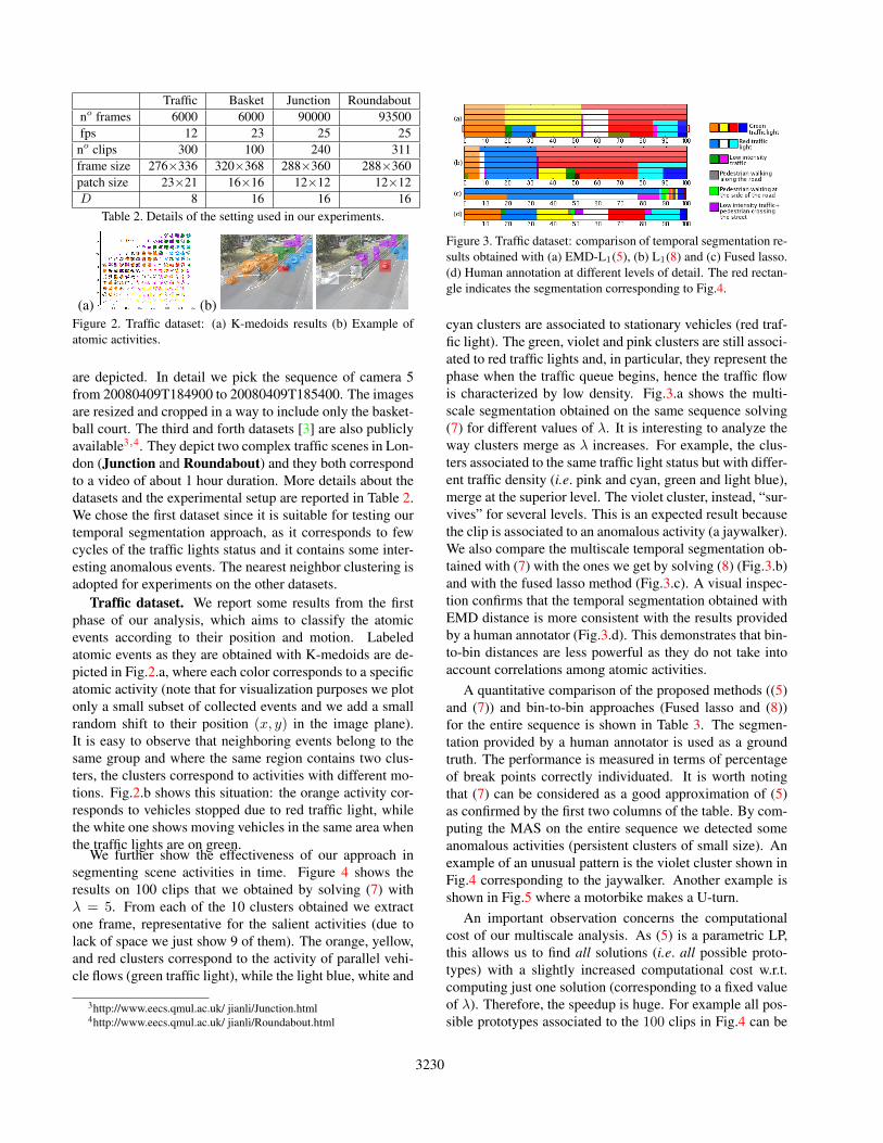
Figure 3. Traffic dataset: comparison of temporal segmentation re-sults obtained with (a) EMD-L1(5), (b) L1(8) and (c) Fused lasso.(d) Human annotation at different levels of detail. The red rectan-gle indicates the segmentation corresponding to Fig.4.

cyan clusters are associated to stationary vehicles (red traf-fic light). The green, violet and pink clusters are still associ-ated to red traffic lights and, in particular, they represent thephase when the traffic queue begins, hence the traffic flowis characterized by low density. Fig.3.a shows the multi-scale segmentation obtained on the same sequence solving(7) for different values of λ. It is interesting to analyze theway clusters merge as λ increases. For example, the clus-ters associated to the same traffic light status but with differ-ent traffic density (i.e. pink and cyan, green and light blue),merge at the superior level. The violet cluster, instead, “sur-vives” for several levels. This is an expected result becausethe clip is associated to an anomalous activity (a jaywalker).We also compare the multiscale temporal segmentation ob-tained with (7) with the ones we get by solving (8) (Fig.3.b)and with the fused lasso method (Fig.3.c). A visual inspec-tion confirms that the temporal segmentation obtained withEMD distance is more consistent with the results providedby a human annotator (Fig.3.d). This demonstrates that bin-to-bin distances are less powerful as they do not take intoaccount correlations among atomic activities.

A quantitative comparison of the proposed methods ((5)and (7)) and bin-to-bin approaches (Fused lasso and (8))for the entire sequence is shown in Table 3. The segmen-tation provided by a human annotator is used as a groundtruth. The performance is measured in terms of percentageof break points correctly individuated. It is worth notingthat (7) can be considered as a good approximation of (5)as confirmed by the first two columns of the table. By com-puting the MAS on the entire sequence we detected someanomalous activities (persistent clusters of small size). Anexample of an unusual pattern is the violet cluster shown inFig.4 corresponding to the jaywalker. Another example isshown in Fig.5 where a motorbike makes a U-turn.

An important observation concerns the computationalcost of our multiscale analysis. As (5) is a parametric LP,this allows us to find all solutions (i.e. all possible proto-types) with a slightly increased computational cost w.r.t.computing just one solution (corresponding to a fixed valueof λ). Therefore, the speedup is huge. For example all pos-sible prototypes associated to the 100 clips in Fig.4 can be

3230

Figure 4. Traffic dataset: (top) salient activities and (bottom)EMD-L1(7) results.

Figure 5. Anomaly: U-turn of a motorbike.

EMD (5) EMD-L1(7) L1(8) Fused Lasso83.2 82.4 72.5 68.7

Table 3. Temporal segmentation accuracy for the traffic dataset

computed in approximately 5 minutes whilst the solutionfor just one value of λ takes about 1 minute.

Basket dataset. We chose this dataset to demonstratethat the proposed approach can be used for applicationsother than traffic scene analysis, such as to obtain a roughsynthesis and useful statistics of a sport match. In par-ticular in the APIDIS sequence five main activities canbe identified: (A) when the yellow team is on defenceand the blue team is trying to shot, (B) when the playersare moving from the yellow team’s court side to the blueteam’s side, (C) when the yellow team is on the defence,(D) when the players are moving back towards the yellowteam’s side. Moreover, due to the asymmetric dispositionof the camera w.r.t. the basketball court, different phases ofthe match can be observed when players are in the yellowteam’s side, such as the case of free throws (E). A repre-sentative frame for each of the five activities as they areautomatically extracted by our algorithm (7) is shown inFig.6(top). Furthermore, Fig.6(bottom) compares the re-sults (i.e. cluster assignments) for 100 clips obtained with(7) and the ground truth. The ground truth is taken fromthe APIDIS website. In detail, we select the timestamps ofannotated events (e.g. ‘Ball possession’, ‘Lost-ball’, ‘Free-throw’,‘Rebound’, etc.) and consider them as breakpoints.We also added some missing breakpoints, e.g. the ones rep-resenting a switch from events B to C or from D to A.

Table 4 shows the results of a quantitative evaluation of

Figure 6. Basket dataset: (top) salient activities and (bottom) (a)EMD-L1(7) results, (b) ground truth.

no clusters EMD-L1(7) L1(8) pLSA pLSA-bin5 90.84 75.17 83.5 77.52 98.42 98.42 94.15 92.25

Table 4. Clustering accuracy (percentage of correctly labeled clips)for the basket dataset

our method (7) compared to (8) and to probabilistic LatentSemantic Analysis (pLSA) with binary and tf-idf featuresrepresentation. PLSA has been chosen as a baseline sinceit has been extensively used in previous works [12, 6]. Weconsider the results for 2 and 5 clusters. In case of the 2clusters the ground truth is created by merging the activi-ties A and E on one side, fusing B, C and D on the other.Table 4 confirms the advantages of EMD-L1 w.r.t. com-peting methods. For example, in case of the 5 clusters (7)outperforms the best competing method with 7% more ofaccuracy. Moreover it is worth noting that pLSA results de-pends upon initialization conditions, as training relies on anon-convex problem.

London’s traffic datasets. We chose these datasetssince they have been extensively used in previous works[3, 4, 5, 6]. However few of them provide the ground truthannotations and quantitative results. One of the few excep-tions is [5]. Table 5 compares the results in [5] with thosewe get on the same data (and same clip size) by applying(7) with P = 3. On both datasets the proposed algorithmoutperforms both pLSA and hierarchical pLSA used in [5].It is interesting to observe that choosing a suitable orderof atomic activities when constructing histograms is cru-cial: using a random order the performance decreases sig-nificantly. These results refer to the situation where onlytwo salient activities are considered. Fig.7 shows an exam-ple of the typical activities for the dataset Roundabout.

We also apply (7) for individuating more than two salientactivities. In this case we only provide a qualitative evalua-tion since quantitative results are not available in literature.For the Junction dataset (Fig.8, top) we discover three mainactivities which correspond to different phases of the trafficflow: A) vertical flow and B) and C) respectively horizontaltraffic flow from right to left and from left to right. Theseactivities are also found in [3, 4], with the difference that in

3231

Figure 7. Roundabout dataset: example of typical activities.EMD-L1(7) L1(8) EMD-L1(7) Standard Hierarchical

random pLSA [5] pLSA [5]J 92.36 89.74 86.7 89.74 76.92R 86.40 86.40 72.3 84.46 72.30

Table 5. Clustering accuracy (%) for Junction (J) and Roundabout(R) datasets

[3, 4] the cluster A is split in two different activities, corre-sponding to vertical flow with and without interleaved turn-ing traffic. This division is less evident as it is confirmed bythe transition behavior matrix in Fig.3.e in [3]. In fact, withour algorithm these patterns emerge when refining the anal-ysis with more than three clusters. Finally we show someexamples of anomalous activities (Fig.8, middle) found byMAS analysis (Fig.8, bottom). Anomalous activities corre-sponding to persistent small size clusters show the momentswhere the traffic lights are on green and vehicles have tostop as a pedestrian is crossing the street (clip 27) and a fire-man truck is passing (clip 83). The last case (clip 98) corre-sponds to a rare event where two large vehicles are passingat the same time. These results, similar to those in [5, 6],confirm the validity of MAS analysis in finding anomalousevents. In our experiments the MAS is computed consider-ing L = 9 subsequent levels of segmentation. However,with large values of L, more accurate MAS profiles canbe obtained, at the expenses of an increased computationalcost. How the anomaly detection performance is affectedby L will be investigated in future works.

5. ConclusionsWe proposed a novel multiscale approach for discov-

ering activity patterns in complex scenes. By taking intoaccount correlations amongst atomic activities, typical pat-terns can be extracted with improved accuracy w.r.t. pre-vious methods. Moreover, if we also learn the temporaldependencies among behaviors, as other state-of-the-art ap-proaches do, we believe that the potential of our methodwill be even better exploited. We leave this to future works.

The main novelty of this paper is the EMD prototypelearning algorithm: we used for dynamic scene understand-ing, but we believe that it could be deployed in other tasks,such as facial expression analysis or action recognition.

References[1] D. Bertsimas and J. N. Tsitsiklis. Introduction to linear opti-

mization. 1997. Athena Scientific. 3225, 3226

Figure 8. Junction dataset. Three salient activities (top), detectedanomalies (middle) and the associated MAS plot and EMD-L1

clustering results (bottom).

[2] J. Friedman, T. Hastie, H. Hofling, and R. Tibshirani. Path-wise coordinate optimization. Annals of Applied Statistics,1:302–332, 2007. 3228

[3] T. Hospedales, S. Gong, and T. Xiang. A markov clusteringtopic model for mining behaviour in video. ICCV, 2009.3225, 3226, 3230, 3231, 3232

[4] D. Kuettel, M. D. Breitenstein, L. V. Gool, and V. Ferrari.What’s going on? Discovering spatio-temporal dependenciesin dynamic scenes. CVPR, 2010. 3225, 3226, 3231, 3232

[5] J. Li, S. Gong, and T. Xiang. Global behaviour inferenceusing probabilistic latent semantic analysis. BMVC, 2008.3231, 3232

[6] J. Li, S. Gong, and T. Xiang. Scene segmentation for be-haviour correlation. ECCV, 2008. 3226, 3231, 3232

[7] H. Ling and K. Okada. An efficient Earth Mover’s Distancealgorithm for robust histogram comparison. IEEE Trans. onPAMI, 29(5):840–853, 2006. 3225, 3228

[8] K. Murty. Linear programming, 1983. Wiley, NY. 3225,3226, 3229

[9] Y. Rubner, C. Tomasi, and L. Guibas. The Earth Mover’sDistance as a metric for image retrieval. IJCV, 40(2):99–121, 2000. 3225, 3226

[10] L. Rudin, S. Osher, and E. Fatemi. Nonlinear total variationbased noise removal algorithms. Phys., 60:259–268, 1992.3228

[11] C. Stauffer and W. Grimson. Adaptive background mixturemodels for real-time tracking. CVPR, 2(1):246–252, 1999.3226

[12] J. Varadarajan, R. Emonet, and J.-M. Odobez. Probabilisticlatent sequential motifs: Discovering temporal activity pat-terns in video scenes. BMVC, 2010. 3225, 3226, 3231

[13] T. Xiang and S. Gong. Video behavior profiling for anomalydetection. IEEE Trans. on PAMI, 30(5):893–908, 2008. 3225

[14] Y. Yang, J. Liu, and M. Shah. Video scene understandingusing multi-scale analysis. ICCV, 2009. 3225, 3226

[15] Y. Yao and Y. Lee. Another look at linear programming forfeature selection via methods of regularization. 2007. Techn.Report 800, Dept. of Statistics, Ohio State University. 3229

3232