Coastal Carolina UniversityCCU Digital Commons

Electronic Theses and Dissertations College of Graduate Studies and Research

7-31-2018

Holocene Formation History of Mud Depocenterson the Continental Shelf in the Gulf of Cadiz,Southwestern SpainMary Lee KingCoastal Carolina University

Follow this and additional works at: https://digitalcommons.coastal.edu/etd

Part of the Geology Commons

This Thesis is brought to you for free and open access by the College of Graduate Studies and Research at CCU Digital Commons. It has been acceptedfor inclusion in Electronic Theses and Dissertations by an authorized administrator of CCU Digital Commons. For more information, please contactcommons@coastal.edu.

Recommended CitationKing, Mary Lee, "Holocene Formation History of Mud Depocenters on the Continental Shelf in the Gulf of Cadiz, SouthwesternSpain" (2018). Electronic Theses and Dissertations. 29.https://digitalcommons.coastal.edu/etd/29

  

HOLOCENE FORMATION HISTORY OF MUD DEPOCENTERS ON THE

CONTINENTAL SHELF IN THE GULF OF CADIZ, SOUTHWESTERN SPAIN

By

Mary Lee King

________________________________________________________________________

Submitted in Partial Fulfillment of the

Requirements for the Degree of Master of Science in

Coastal Marine and Wetland Studies in the

School of the Coastal Environment

Coastal Carolina University

July 2018

Dr. Till J.J. Hanebuth, Major Professor

______________________________

Dr. Francisco Lobo (IACT)

______________________________

Dr. Jenna Hill (USGS)

______________________________

Dr. Richard Viso, SCE Director

______________________________

Dr. Isabel Mendes (UAlg)

______________________________

Dr. Richard Viso (CCU)

______________________________

Dr. Michael H. Roberts, Dean

______________________________

  

Copyright

© 2018 by Mary Lee King (Coastal Carolina University)

All rights reserved. No part of this document may be reproduced or transmitted in any form or by any means, electronic, mechanical, photocopying, recording, or otherwise, without prior written permission of Mary Lee King (Coastal Carolina University).

iii  

Acknowledgements

First and foremost, this thesis could not have been conducted without my outstand-

ing committee, data from research cruise POS482 CADISED on the German RV POSEI-

DON, and numerous institutions that provided support through funding or data collection.

MARUM – Center of Marine Environmental Sciences at the University of Bremen in Ger-

many provided funding for the POS482 CADISED research cruise. Collaborators are from

Andalusian Institute of Earth Sciences (IACT) as part of Consejo Superior de Investi-

gaciones Científicas (CSIC) of Spain, Instituto Geológico y Minero de España (IGME),

Madrid, Spain, under the Ministry of Economy and Competitiveness, University of Al-

garve (UAlg) in Faro, Portugal, Coastal Carolina University (CCU), and United States Ge-

ologic Survey (USGS) in Santa Cruz, California. The productive scientific crew headed by

chief scientist Dr. Till Hanebuth (CCU), included Dr. Francisco Lobo (IACT/CSIC), Dr.

Isabel Mendes (UAlg), Dr. Isabel Reguera (IGME), Dr. María Luján (IACT), PhD candi-

date Fenna Bergmann (MARUM), PhD candidate Grit Warratz (MARUM), MSc candi-

dates Bastian Steinborn (MARUM), and Matthew Kestner (CCU). I would also like to

acknowledge the outstanding professional crew of the RV POSEIDON.

Thank you to my committee for their constant support and guidance. Dr. Isabel

Mendes (UAlg) and Dr. Francisco Lobo (IACT/CSIC) provided an abundant, never ending

supply of new insightful references concerning sediment characteristics, human impacts,

and paleoenvironmental climatic conditions. Seismio-acoustic interpretation assistance and

software availability were supported by Dr. Jenna Hill (USGS) and Dr. Rich Viso (CCU).

Special thank you to Dr. Till Hanebuth (CCU) for taking a chance and first meeting me in

person days before the POS482 CADISED research cruise in Portugal. His mentorship,

iv  

continued encouragement, and willingness to provide constant advice will attribute to my

future success in my scientific career.

In addition to being a committee member, Dr. Francisco Lobo (IACT/CSIC) gra-

ciously provided funding for a third of 14C sample analysis. Samples were analyzed for

210Pb concentration by Ferdinand Oberle from (USGS). Dr. Lebreiro (IGME) and her re-

search group also provided 14C, 210Pb, and 137Cs ages for use in this thesis.

I would also like to acknowledge Dr. Hendrik Lantzsch (MARUM) and other col-

lages from University of Bremen for organizing lab time and data collected in facilities.

Element powder concentrations were collected by Dr. Matthias Zabel. Total organic con-

tent and carbonate concentrations were analyzed by Brit Kockisch. Vera Barbara Bender

and Vera Lukies provided assistance in the GeoB Core Repository and XRF element scan-

ning. Scientific and social support was also thankfully provided by Grit Warratz, Bastian

Steinborn, Mareike Höhne, and Fenna Bergmann while I was in Germany.

This incredible project couldn’t have been completed without the constant support

and encouragement from collaborators, friends, and family. Thank you to Ashley Long

(CCU) for her advice and seemingly never ending knowledge of Kingdom Suite software.

I would also like to acknowledge numerous other graduate students, friends, and family for

being there to share the good and bad times with. Thank you to my parents and brothers

for supporting my goals and aspirations.

v  

Abstract

Holocene mud accumulation on the continental shelf in northern Gulf of Cadiz,

from the Guadalquivir River to the Tinto-Odiel Estuary, is described as two types of mud

depocenters (MDCs): a sheet-like prodelta and mud belt. Despite a substantial number of

investigations of this continental shelf (Somoza et al., 1997; Hernández-Molina et al.,

2000; Lobo et al., 2001; synthesis: Lobo et al., 2015), information on Holocene sediment

facies and a robust stratigraphic age model remained unestablished (Lobo et al., 2002; and

Lobo and Ridente, 2014). Objectives of this study are to describe the dynamics of MDC

formation in a chrono- and litho-stratigraphic approach as well as to calculate a sediment

budget. Research cruise POS482 on the German RV Poseidon collected 2,040 km of

seismo-acoustic profiles and forty sediment cores in March 2015 with collaborative part-

ners of the CADISED project. X-ray fluorescence core scanning, used in combination with

magnetic susceptibly, porosity, high resolution core imaging, lithology description, and

radiography depict five successive sedimentary facies since 9.0 cal ka BP. Boomer data

sets from 1992 and 1986 combined with new CADISED seismo-acoustic profiles provide

detailed insight to the geometric formation of this depocenter. Of particular surprise is that

the sheet-like prodelta MDC is locally subsiding as a result of semi-recent active extension

faults related to local salt diapir uplift. 14C and 210Pb dating provide an age control to the

history of mud accumulation. Grain density and sedimentation rates determine accumula-

tion trends in the range of 0.03 to 0.46 grams per cubic millimeter a year (g mm-2 yr-1) from

early Holocene times until 2.7 cal ka BP. The following 1500 yrs show rates increasing by

up to ninety times (0.32 to 2.66 g mm-2 yr-1), correlating with a widespread humid climate

period from 2.6 to 1.6 cal ka BP and enhanced mining and agricultural activity by the

vi  

Roman Empire. Since 1.0 cal ka BP, accumulation rates increase even further due to in-

dustrialization and intense land use (1.09 to 28.63 g mm-2 yr-1). Smaller climatic events

also contributed to changes in sediment accumulation. For example, the Medieval Climate

Anomaly (MCA) coincided with a decrease from 1.05 to 0.7 cal ka BP. The total volume

of the MDCs is 5.80 km3 with a total and dry sediment mass of 12,971 Mt. Total Organic

Content (TOC) mass of 85 Mt and a 0.038 km3 volume with a CaCO3 mass of 3,637 Mt

and a 1.63 km3 volume makes this depocenter an important quasi-modern sink in the ma-

rine sector of the regional carbon cycle.

vii  

Table of Contents Acknowledgements .......................................................................................................... iii

Abstract ...............................................................................................................................v

1.0 Introduction .............................................................................................................1

2.0 Background – Northern Gulf of Cadiz Continental Shelf ..................................3

2.1 Mud Depocenter Classification ............................................................................ 3

2.2 Holocene Sea Level History and Response of the Sedimentary System ............... 5

2.3 The Holocene as a Climatic Epoch ...................................................................... 6

2.4 Regional Oceanographic Currents ...................................................................... 9

2.5 Fluvial Sources – Characterization and Geologic Foundation ......................... 11

2.6 Shelf Characteristics and Stratigraphy .............................................................. 14

3.0 Objectives and Research Questions ....................................................................16

3.1 Chrono- and Lithostratigraphy of Mud Depocenters ........................................ 16

3.2 Budget Calculation of Mud Depocenters ........................................................... 17

4.0 Materials and Methods .........................................................................................18

4.1 Seismo-Acoustic Data ........................................................................................ 19

4.2 Multi-Sensor Core Logger (MSCL) Data ........................................................... 20

4.3 Sediment Properties and Budget Calculation .................................................... 20

4.4 X-ray Fluorescence Element Scanning .............................................................. 22

4.4.1 Element Intensity Ratios ............................................................................. 22

4.4.2 X-ray Fluorescence Powder Element Measurement ................................... 24

4.5 14C Dating .......................................................................................................... 24

4.6 210Pb and 137Cs Dating ....................................................................................... 25

4.7 High-Resolution Core Imaging .......................................................................... 26

5.0 Critical Evaluation of Stratigraphic Age Model and Material Budgets ..........27

5.1 Calculation of Sedimentation Rates ................................................................... 27

5.2 Calculation of Material Budgets ........................................................................ 29

6.0 Results ....................................................................................................................30

6.1 Age framework ................................................................................................... 30

6.2 Determination and Timing of Sedimentary Facies ............................................ 30

6.3 Stratigraphic Architecture.................................................................................. 34

6.4 Material Budget Calculation .............................................................................. 38

6.5 Carbon Budget Calculation ............................................................................... 38

viii 

7.0 Interpretation and Discussion ..............................................................................40

7.1 Mud Depocenter Evolution: Influences on Accumulation and Stratigraphy ..... 40

7.1.1 Holocene Transgression to 6.5 cal ka BP ................................................... 40

7.1.2 Maximum Flooding Surface ........................................................................ 42

7.1.3 Highstand Depositional System .................................................................. 42

7.2 Sediment Budget Calculation ............................................................................. 48

7.3 Tectonic Influence on the Geometry of the Mud Depocenter ............................. 50

7.4 Differentiation of Sediment Sources ................................................................... 52

8.0 Conclusions ............................................................................................................54

9.0 Tables .....................................................................................................................58

10.0 Figures ................................................................................................................69

11.0 References ........................................................................................................107

12.0 Appendix ..........................................................................................................155

ix  

List of Tables

Table 1. Justification to use specific data for each Thesis Objective.

Table 2. Justification for stations selected in the study area based on preliminary interpretation of acoustic data. (1)Representative stations used for correlating ele-ment intensity ratios to create a robust age framework for MDCs.

Table 3. Data sets collected at coring stations within study area.

Table 4. Summary of MDCs facies characterization by sediment properties.

Table 5. Sediment cores with coordinates, water depth taken, sediment sample depth in core, measured conventional radiocarbon ages (+1σ error), calibrated radiocarbon ages (+1σ error, calibrated with CALIB software version 7.10 with data set "ma-rine13.14c") (Stuiver and Reimer, 1993; Reimer et al. 2013).

Table 6. Age models for Cores 19534-3, 19520-3, 19512-3, and 19535-3, using 210Pb and 137Cs dating methods. All ages are given in Common Era (CE). Constant Rate of Supply (CRS) and Constant Initial Concentration (CIC) models were used for 210Pb ages.

Table 7. Sedimentation rates (cm ka-1) calculated between two age points using 210Pb pro files and 14C dating. Listed by coring site. Example of how to read the table: The lowermost part of Core 19521 has a sedimentation rate of 12 cm ka-1 from 8.98 to 6.67 cal ka BP.

Table 8. Accumulation rates (g cm-2 ka-1) based on 210Pb profiles and 14C dating. Listed by stations. Example how to read this table: The base of 19521 has an accumulation rate of 16 g cm-2 ka-1 from 8.98 to 6.67 cal ka BP.

Table 9. Summary of MDCs sediment properties by time slice as defined from seismo- acoustic profile analysis.

Table 10. Representative total carbon content (TC), total organic content (TOC), and calcium carbonate content (CaCO3) for MDCs.

Table 11: Comparison of three shelf systems with a confined MDCs, for which a high- resolution budget analysis was performed. (1) This study; (2) Lantzsch et al., 2009; (3) Brommer et al., 2009. Although the base of the MDCs from the Gulf of Cadiz are dated at 10.0 ± 1.0 cal ka BP, the regime change occurred at 6.5 cal ka BP (comparable to the other systems). (*) Calculated number.

x  

List of Figures

Figure 1. The Guadalquivir River in southeastern Spain pushing a sediment filled plume into the northern Gulf of Cadiz on 13 November 2012 (Schmaltz, 2012). The red circle represents the study area for this study.

Figure 2. (A.) Location map of Iberian Peninsula in relation to study area. (B.) Zoomed in to track lines of POS482 echosounder data (black lines). (C.) Study area between the Tinto-Odiel Estuary and Guadalquivir River. Due to map size, Station names were reduced to their representative last two digits: Station 19513 is location 13, etc. Station location numbers that are focused on have a pink background. Figure locations of seismo-acoustic profiles are depicted.

Figure 3. Suspended sediment discharges from a freshwater plume forming a bottom layer that is driven by gravity and bottom currents. This bottom layer either deposits forming MDCs or bypasses the system off the shelf edge (Hanebuth et al., 2015).

Figure 4. Surface distribution of sediment. (A) Faro-Tavira wedge; (B) inner wedges; (C) shelf aggradational deposits (C1: undifferentiated shelf aggradational deposits, C2: shelf muddy belts, or shelf aggradational deposits with elongated patterns; C3: main MDCs of shelf muddy belts); (D) Guadalquivir wedge (Lobo et al., 2004).

Figure 5. Chronostratigraphic framework compiled by correlating seismo-acoustic Gulf of Cadiz images and comparing with peer-reviewed eustatic sea-level curves mod-ified from Fairbanks (1989), Stanley (1995), Hernández-Molina et al. (1994), Bard et al., (1996) (Lobo et al., 2001).

Figure 6 (A). A high-resolution seismo-acoustic profile off the Guadalquivir River. (B). Interpretations of the high-resolution profile depict a TST and the repetition of pro-gradational and aggradational deposition units during the Holocene HST (Lobo et al., 2005; modified from Fernández-Salas et al., 2003). Location of this profile is depicted on Figure 2.

Figure 7. Relative mean sea level curve since 9.0 cal ka BP from the Quarteira coast, in the Gulf of Cadiz, Portugal. Each box is error represented for one sample from lagoon and estuarine sediments. Image modified by Zazo et al. (2008) from Teixeira et al. (2005).

Figure 8. (A.) Hydrologic data from 1966-1992 taken on the Tinto River in Niebla, Spain (B.) Annual discharge patterns monthly from 1966-1992 (modified after Davis et al., 2000, corrected).

Figure 9. Surface circulation patterns of the southwest Iberian Peninsula. N2 and N1 are described by García-Lafuente et al., 2006 as cores of eastward flowing water. N2 is a portion of large-scale circulation current that drives the geostrophic flow around the southeastern Iberian Peninsula from the Portuguese Current, also referred to simply as the NASW (Lobo et al., 2004). N2 flows east through the Strait of Gi-braltar into the Mediterranean or veers south becoming part of the Canary current. N2 is warmer and saltier than N1, suggesting N1 contains water from another body.

xi  

The dashed line at the southeast indicates closure of core N1 with the Coastal Coun-ter Current (CCC). The CCC feeds core N1 in the west, however, under favorable conditions can bypass Cape Santa Maria westward feeding the Cape San Vicente cyclonic eddy (SVE) (García-Lafuente et al., 2006).

Figure 10. Basic Geologic Map of Spain depicting the location of the Guadalquivir basin and insert (a.) depicting in detail the Iberian Pyrite Belt (IPB) composed of three lithological groups: the Phyllite-Quartzite Group, Volcano-Sedimentary Complex (VS), and the Culm Group (Spanish Geological Survey IGME 1998; (a.) Onézime et al., 2003).

Figure 11. Pb/Al ratio concentrations with overlapping human impact time periods that have caused chronological markers as early as the Bronze Age in the Alboran Sea and Zoñar Lake in Spain (Martín-Puertas et al., 2010).

Figure 12. Ln Ti/Fe ratio, comparing two proxy elements used in identifying terrigenous material from cores that include all facies (19535-3, 19538-3, and 19513-3). The 14C ages presented are those collected from the depth portrayed. See Figure 2 for coring station locations.

Figure 13. Interpretive stratigraphic core correlation represented by orange lines of ln (Ca/Fe) from the Tinto-Odiel Estuary to the Guadalquivir River (distal to shore) Cores 19538-3, 19513-3, and 19518-3. The red lines indicate calibrated 14C ages collected from the core. For location of core transect see Figure 2.

Figure 14. Ln Ti/Al ratio, comparing two proxy elements used in identifying terrigenous material from cores that include all facies (19535-3, 19538-3, and 19513-3). The 14C ages presented are those collected from the depth portrayed. See Figure 2 for coring station locations.

Figure 15. Interpretive stratigraphic core correlation represented by orange lines of ln (Ca/Fe) in cores 19534-3, 19535-3, and 19538-3 located perpendicular to shore from the Tinto – Odiel Estuary. The red lines indicate calibrated 14C ages collected from the core.

Figure 16. Combined stratigraphic correlation of element intensity ratios and magnetic susceptibility from stations perpendicular to shore from Tinto-Odiel region to Gua-dalquivir. Numbers above red lines on cores are radiocarbon samples dated in cal ka BP. The same interpretive correlation in Figure 15 of ln Ca/Fe is also represented here by orange lines in correlation 19534-19535-19538. The multi-color grey and white boxes indicate different facies interpretations represented within the cores (Figure 21). Core lengths are indicated by the extent of the facies boxes.

Figure 17. Combined stratigraphic correlation of element intensity ratios and magnetic susceptibility from stations parallel to shore from proximal to distal. Numbers above red lines on cores are radiocarbon samples dated in cal ka BP. The same interpretive correlation in Figure 13 of ln Ca/Fe is also represented here by orange

xii  

lines in correlation 19538-19513-19518. The multi-color grey and white boxes in-dicate different facies interpretations represented within the cores (Figure 21). Core lengths are indicated by the extent of the facies boxes.

Figure 18. Depth – Age representation of sedimentation rates given in thousands of years (cm/ka) for transect near the Guadalquivir River (Site locations: Figure 2). Ages from 210Pb located at tops of cores are given in Common Era (CE). Ages with an asterisk (*) indicate data was extrapolated from seismio-acoustic profiles. For a complete list of sedimentation rates refer to Table 7. Note that depth profiles are not the same size due to differences in rates of sedimentation.

Figure 19. Depth – Age representation of sedimentation rates given in thousands of years (cm/ka) for transect shore-perpendicular through the central portion of the study area (Site locations: Figure 2). Ages from 210Pb located at tops of cores are given in Common Era (CE). For a complete list of sedimentation rates refer to Table 7.

Figure 20. Depth – Age visual representation of sedimentation rates given in thousands of years (cm/ka) for transect shore-perpendicular near the Tinto-Odiel Estuary (Site locations: Figure 2). Ages from 210Pb located at tops of cores are given in Common Era (CE). Ages with an asterisk (*) indicate data was extrapolated from seismio-acoustic profiles. For a complete list of sedimentation rates refer to Table 7. Note that depth profiles are not the same size due to differences in rates of sedimentation.

Figure 21. Idealized profile and lithology descriptions of the successive sedimentary fa- cies units (A – F) synthesized from the sediment cores collected. Yellow ages are the range at which the facies boundaries are present in cores, depending on core location and accumulation rate. Ages listed next to the core image of 19538-3 were amassed through the age model created for site 19538 and fall within facies bound-ary age ranges. Ln Ti/Zr ratio depicts a fining upward of sediment. Ln Ca/Fe ratio shows a general increasing trend of terrigenous material up core. Sequence strati-graphic interpretation includes transgressive systems tract (TST), maximum flood-ing surface (mfs), and highstand systems tract (HST).

Figure 22. Ln Ti/Zr ratio used as a grain size proxy. Depth axis are not depicted by the same scale to clearly show similar grain size trends from cores that include all facies (19535-3, 19538-3, and 19513-3). The 14C ages presented are those collected from the depth portrayed. See Figure 2 for coring station locations.

Figure 23. Photos from selected cores illustrating sedimentary facies of mud accumula- tion of MDCs on the continental shelf in the Gulf of Cadiz, Southwestern Spain.

Figure 24. Compilation of the 98 accumulation rates from MDCs. The green background envelope includes accumulation rates from the prodelta MDC and the purple of the mud belt MDC. Three high accumulation rates from modern deposition are not shown to depict in greater detail older accumulation rates. Two rates from 4.72 to 1.95 cal ka BP and one rate from 1.95 to 0.88 cal ka BP were not used in the prodelta MDC envelope due to the higher error associated with the seismio-acoustic extrap-olated ages. Low accumulation rates were persistent until 2.7 to 0.4 cal ka BP when

xiii  

the rates increased to about 1.4 g mm-2 ka-1. From 0.4 cal ka BP to present, accu-mulation rates increased exponentially to as high as 29 g mm-2 ka-1.

Figure 25. (A.) Seismo-acoustic profile and (B.) with interpretations, depicting Holocene mud accumulation near the Tinto-Odiel estuary. The zoomed-in section shows in high-resolution the internal stratification of the mud belt MDC. Major horizons are traced and correspond to the age model collected from 14C dates. Location of this profile is depicted on Figure 2.

Figure 26. (A.) Seismo-acoustic profile and (B.) with interpretations, depicting Holocene mud accumulation of the northwestern portion of the prodelta MDC, shore-perpen-dicular. The zoomed-in section shows in high-resolution the internal stratification around mud entrapments. Major horizons are traced and correspond to the age model collected from 14C dates. Location of this profile is depicted on Figure 2.

Figure 27. Notable features relating to the MDCs overlain on ship track lines and station locations. The faults labeled are found only within the Holocene sediment. Faults associated with Structures are speculative. The prodelta MDC is centrally located near two acoustically masked locations. The southwestern acoustically masked area is below the Holocene sediment. There are deeper extension faults located in cor-relation with diapirs.

Figure 28. (A.) Seismo-acoustic profile and (B.) with interpretations, depicting Holocene mud accumulation of the southeastern portion of the prodelta MDC, shore-perpen-dicular. The zoomed-in section shows in high-resolution the internal stratification are traced and correspond to the age model collected from 14C dates. Horizons stop at acoustic masking locations. Location of this profile is depicted on Figure 2.

Figure 29. Mud Belt MDC (coring sites 19534, 19535, 19538) and Prodelta MDC (coring sites 19512, 19513, 19518, 19519, 19520, 19521) central depositional locations outlined by contour thickness of 6 m. Coring sites are distinguished by blue dots.

Figure 30. Isopach map of the MDCs from stratigraphic base to modern seafloor. Blue dots are coring locations for reference.

Figure 31. (Profile A) One lobe of the eastern diapiric uplift, close to the Guadalquivir River, 40 m from mean sea level. (Profile B) The cap rock of the diapir has pene-trated the base of the prodelta MDC, 3 m from seafloor. Location of seismio-acous-tic profiles in Figure 2.

Figure 32. Western diapir with related extension faults, located near shelf edge below the base of the prodelta MDC. Location of seismio-acoustic profile in Figure 2.

Figure 33. Isopach map from the base of the MDCs to sediment horizon dated at 2.0 ± 0.1 cal ka BP (Slice 1). Blue dots are coring locations for reference.

Figure 34. Isopach map from sediment reflector dated at 2.0 ± 0.1 cal ka BP to sediment reflector dated at 1.0 ± 0.1 cal ka BP (Slice 2). Blue dots are coring locations for reference.

Figure 35. Isopach map from sediment reflector dated at 2.0 ± 0.1 cal ka BP to modern

xiv  

seafloor (Slice 2.5). Blue dots are coring locations for reference.

Figure 36. Isopach map from sediment reflector dated at 1.0 ± 0.1 cal ka BP to modern seafloor (Slice 3). Blue dots are coring locations for reference.

Figure 37. Entrapping structures subsiding as a result of overbearing sediment weight causing major horizons and prodelta MDC base to dip towards the central accumu-lation center of the depocenter. Location of seismio-acoustic profile in Figure 2.

Figure 38. Comparison of sedimentation rate trend from the MDCs (orange line), based on sediment cores in this study, with an idealized sedimentation rate trend from estuaries (blue line), modified from Lario et al. (2002). (For accumulation rates for this study, see Figure 23).

Figure 39. Evidence of block-like subsidence occurring between the two main diapir lo cations affecting the prodelta MDC. Location of seismio-acoustic profile in Figure 2.

Figure 40. Acoustic masking due to the presence of gaseous sediments near the western diapir along the shelf edge. Location of seismio-acoustic profile in Figure 2.

1  

1.0 Introduction

Fluvial sources supply the majority of continent derived, fine grained sediment to

a continental shelf. If adequate ocean currents exist, further transport of sediment will occur

until currents dissipate, allowing for deposition. These depositional locations, commonly

described as mud depocenters (MDCs) or mudbelts, form during periods of slow sea level

change or standstill (Hanebuth et al., 2015a).

The study area is confined to the northeastern Gulf of Cadiz in water depths ranging

from 15 to 200 m. The Gulf of Cadiz shelf has a diverse depositional system with multiple

fluvial sources of sediment influx (Lobo et al., 2004). The Guadalquivir River is the main

source, delivering a large sediment plume, altered by ocean currents (Figure 1). Previous

studies on the shelf, near on the Guadalquivir River, depict transgressive units overlain by

two sequences of progradational and aggradational units in the Holocene highstand sys-

tems tract (Lobo et al., 2005).

The interplay between sediment supplied by several rivers, a complex ocean current

system, climatic events, fluctuating sea level, and anthropogenic modifications on land can

control the depositional architecture of highstand MDCs on the continental shelf in the

northeastern portion of the Gulf of Cadiz, Spain. Previous investigations of MDCs in the

Gulf of Cadiz have relied almost exclusively on subbottom echosounder data (Lobo et al.,

2001, 2002, 2004, 2005; synthesis: Lobo et al., 2015). The seismic stratigraphic architec-

ture has been generally described in several studies (Somoza et al., 1997; Hernández-Mo-

lina et al., 2000; Lobo et al., 2001; synthesis: Lobo et al., 2015; Lobo and Ridente, 2014).

2  

Despite a substantial number of investigations in the Gulf of Cadiz, information on sedi-

ment facies types and accumulation rates from the Holocene are limited by location (Gua-

diana: Mendes et al., 2010, 2012; Martins et al., 2012) or by age coverage and resolution

(Nelson et al., 1999; Abrantes et al., 2017). The first objective of this master’s thesis is to

fill that void by investigating the chrono- and litho- stratigraphy based on a set of sediment

cores in combination with seismo-acoustic data sets, while speculating on mechanisms

controlling sediment deposition. The other objective is to devise volume and mass budget

calculations for the Gulf of Cadiz MDCs.

This thesis will utilize an extensive seismo-acoustic data set and eighteen marine

sediment gravity cores to determine the formation history of confined shelf MDCs related

to the Guadalquivir River and various other surrounding sources. Subbottom echosounder

profiles and sediment cores were collected on March 14-25, 2015 during RV Poseidon

cruise POS482 CADISED (Cadiz Shelf Sediment Depocenters), providing excellent data

coverage for this study (Figure 2). Gravity cores and sediment samples are compared to

the seismo-acoustic data set and analyzed for magnetic susceptibility, porosity, density,

element intensity distribution, element concentrations, radiocarbon (14C) dates, and Lead-

210 (210Pb) and Cesium-137 (137Cs). These analyses provide a basis for development of

age models leading to detailed insight of centennial through millennial changes of shelf

mud accumulation patterns, driven by climatic changes and anthropogenic industrial-scale

advancements.

3  

2.0 Background – Northern Gulf of Cadiz Continental Shelf

2.1 Mud Depocenter Classification

MDC formation begins as freshwater and sediment discharges from a fluvial source

onto the continental shelf creating a freshwater plume (Figure 3). Sediment falls out of

suspension from the plume to form a distinct turbid (nepheloid) bottom layer, driven

mainly by bottom currents and gravity (Figure 3; Hanebuth et al., 2015a). Through shelf

currents, gravity forcing of the nepheloid layer, wave and tidal action, sediment either de-

posits, forming MDCs or bypasses them across the shelf break (Hill et al., 2007; Hanebuth

et al., 2015a).

Although there are many ways to classify a MDC, there are some common traits

used to define them. A MDC must have at least a 25% mud concentration (George and

Hill, 2008), whereas mud is defined as material that is < 63 micrometers (μm) (McCave,

1972) which is a mixture of silt and clay. Most MDCs contain a mixture of sand, silt, and

clay with an occasionally strong silt fraction (Hanebuth and Lantzch, 2008).

MDCs form differently on continental shelves due to shelf gradient, sediment dis-

charge from fluvial sources, local hydrodynamic forcing, current strength and direction,

and sea level rise or stand still. Walsh et al., 2009 defined a hierarchical tree to predict

marine accumulation systems at most river mouths using morphologic and oceanographic

characteristics. Their system relies on having knowledge of the sediment quantity dis-

charged per yr, shelf width, and wave and tidal conditions in the area. Depocenter locations

can rapidly shift in response to short-term sea-level fluctuations (Hanebuth et al., 2011).

4  

Hanebuth et al. (2015a) defined eight different kinds of MDCs: prodelta, subaqueous del-

tas, mud patches, mud blankets, mud belts, shallow-water contourite drifts, mud entrap-

ments, and mud wedges. Walsh et al., 2009 defined additional locations of deposition, such

as a canyon or past the shelf break. For this study, the focus is on prodelta, mud blankets,

mud belts, and mud entrapments due to an abundant terrestrial sediment supply and previ-

ous morphological characterization of MDCs on this shelf (Lobo et al., 2004, 2005; Hane-

buth et al., 2015a).

Sheet-like prodelta MDCs are attached to a fluvial point source pinching-out sea-

ward (Hanebuth et al., 2015a). A MDC formed by the Guadalquivir River in the Gulf of

Cadiz has been identified as a prodelta type due to mainly aggradational trends found

within seismo-acoustic data (Figure 4; Fernández-Salas et al., 2003; Lobo et al., 2004,

2005). Analysis of these seismo-acoustic profiles depicts alternating sequences of progra-

dational deposits overlain by aggradational subunits (Lobo et al., 2005).

Rarely found mud blankets have extensions that are near to sediment source with

equal shelf-wide and sheet-like sediment distribution in various directions (Hanebuth et al.,

2015a). Acoustic profiles of mud blankets, either attached to the point source or closely

associated, depict a more or less constant thickness over the continental shelf (Hanebuth et

al., 2015a). The MDC formed by the Guadalquivir River has also been described as having

mud blanket like shelf-wide extensions (Lobo et al., 2004).

Mud belts are elongated sediment bodies with aggradational deposition thinning

seaward and typically form parallel to bathymetry with detachment from the point source

(Hanebuth et al., 2015a). The shelf off Galicia in northwest Spain and parts of the Gulf of

5  

Cadiz (Figure 4) are examples of classic mud belts (Fernández-Salas et al., 2003; Lobo et

al., 2004, 2005; Hanebuth et al., 2015a).

Locally defined mud entrapments occur where sediment becomes trapped around

an obstacle or in a depression on the seafloor. Mud entrapments contain a planar surface

and show a homogeneous to slightly horizontal internal stratification (Hanebuth et al.,

2015a). Acoustic profiles of mud entrapments also depict detachment from point source

with sheet to trough-like fill (Lantzsch et al., 2009; Hanebuth et al., 2015a).

2.2 Holocene Sea Level History and Response of the Sedimentary System

High-resolution seismic stratigraphy at various shelf locations depicts inconsistent

sea-level changes, during the Holocene (Lobo et al., 2001, 2002, 2004, 2005), owing to

localized isostatic effects (Hernández-Molina et al., 1994). Lobo et al. (2001) proposed a

chronostratigraphic framework for Gulf of Cadiz shelf deposits based upon correlation of

seismo-acoustic data with eustatic sea-level curves from Fairbanks (1989), Stanley (1995),

Hernández-Molina et al. (1994), and Bard et al. (1996) (Figure 5). The trend of all these

sea-level curves indicates the Iberian Peninsula experienced sea-level rise during the early

Holocene and slow sea-level rise or standstill during the late Holocene (Figure 5; Lobo et

al., 2001).

Sea level rose relatively fast after 11.7 cal ka BP (start of the Holocene) with inter-

mittent moments of sea level stability due to melting of high latitude icecaps (Bird et al.,

2007) to a point around 8.0 cal ka BP (MWP-2 – Alley et al., 1997; Bird et al., 2007). The

filling of incised valleys and continued shoreline retrogradation, during rapid sea level rise,

is described as being part of a transgressive systems tract (TST) (Van Wagoner et al., 1988).

A TST is preserved on the Gulf of Cadiz shelf by localized sediment beds deposited at fast

6  

rates or areas of little accumulation (Figure 6; Van Wagoner et al., 1988; Lobo et al., 2001,

2004). A period of deceleration in sea level rise occurred from about 8.0 cal ka BP until

6.5 cal ka BP, when sea level began to stabilize forming a maximum flooding surface (mfs)

(Figure 7; Dabrio et al., 2000; Lario et al., 2002; Zazo et al., 2008 from Teixeira et al.,

2005). A mfs occurs when sea level reaches its highest point in flooding the continental

shelf (Van Wagoner et al., 1988) and is associated in the Gulf of Cadiz shelf with a con-

densed sedimentological record (Dabrio et al., 2000; Lario et al., 2002).

After 6.5 cal ka BP, sea level stabilized to the present position (Figure 7; Dabrio et

al., 2000; Lario et al., 2002; Zazo et al., 2008 from Teixeira et al., 2005), allowing a high-

stand unit (HST) form with a depositional geometry characterized by aggradational and

progradational clinoforms (Van Wagoner et al., 1988; Lobo et al., 2005). HST occurs dur-

ing the latest portion of sea level rise, standstill, and the early portion of following sea level

fall (Van Wagoner et al., 1988).

2.3 The Holocene as a Climatic Epoch

Climate variability in the Holocene is characterized by intervals of polar cooling,

solar variability, and changes in atmospheric circulation (Mayewski et al., 2004). Prevail-

ing winds in southern Iberia from 10 to 6.45 cal ka BP changed direction from SW to W

prompting paleocurrents to flow NE to E (Goy et al., 1996). Eolian dune preservation from

6.45 to 3 cal ka BP indicates prevailing winds drastically changed direction causing paleo-

currents to flow in a W direction. For a brief time (3 to 2.75 cal ka BP), prevailing winds

shifted significantly causing paleocurrent flow direction to flip from W to E. Since 2.75 cal

ka BP, a strong fluvial influence on sedimentation, indicates strong rain in short periods

under drought-like conditions (Goy et al., 1996).

7  

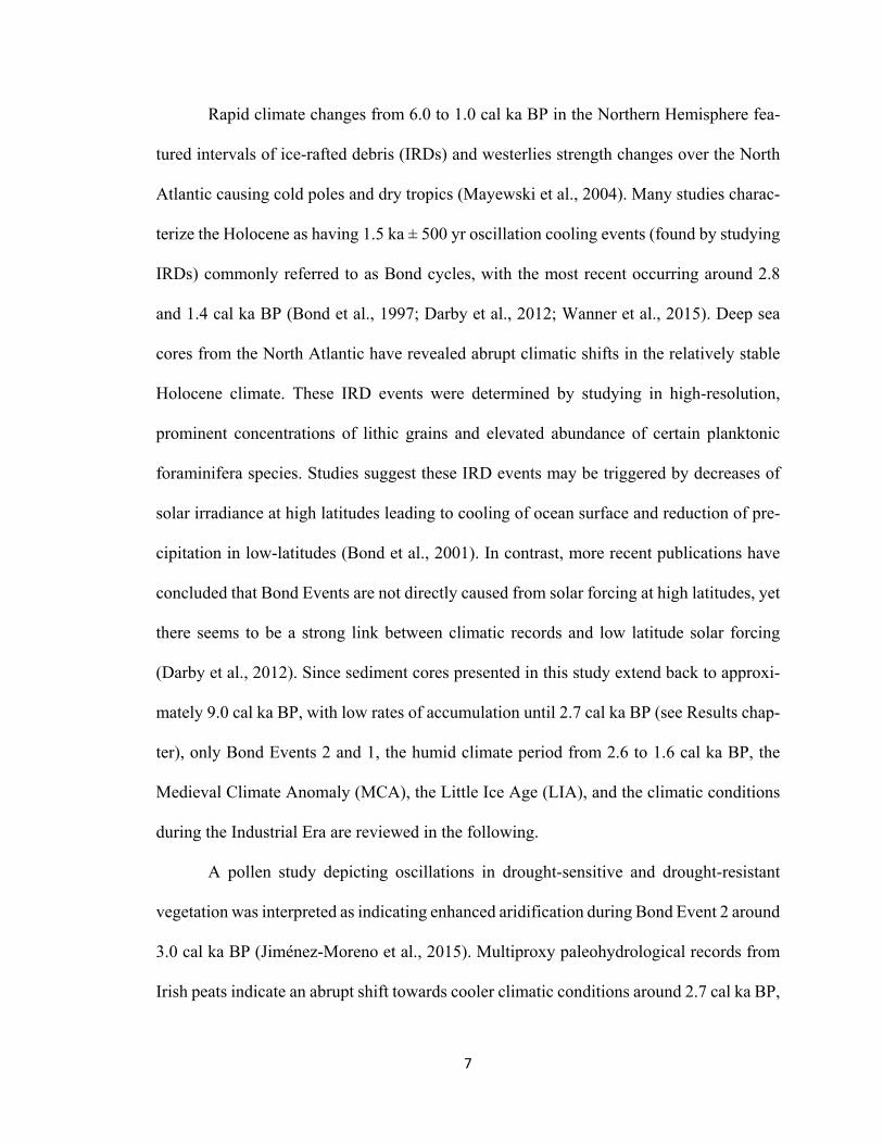
Rapid climate changes from 6.0 to 1.0 cal ka BP in the Northern Hemisphere fea-

tured intervals of ice-rafted debris (IRDs) and westerlies strength changes over the North

Atlantic causing cold poles and dry tropics (Mayewski et al., 2004). Many studies charac-

terize the Holocene as having 1.5 ka ± 500 yr oscillation cooling events (found by studying

IRDs) commonly referred to as Bond cycles, with the most recent occurring around 2.8

and 1.4 cal ka BP (Bond et al., 1997; Darby et al., 2012; Wanner et al., 2015). Deep sea

cores from the North Atlantic have revealed abrupt climatic shifts in the relatively stable

Holocene climate. These IRD events were determined by studying in high-resolution,

prominent concentrations of lithic grains and elevated abundance of certain planktonic

foraminifera species. Studies suggest these IRD events may be triggered by decreases of

solar irradiance at high latitudes leading to cooling of ocean surface and reduction of pre-

cipitation in low-latitudes (Bond et al., 2001). In contrast, more recent publications have

concluded that Bond Events are not directly caused from solar forcing at high latitudes, yet

there seems to be a strong link between climatic records and low latitude solar forcing

(Darby et al., 2012). Since sediment cores presented in this study extend back to approxi-

mately 9.0 cal ka BP, with low rates of accumulation until 2.7 cal ka BP (see Results chap-

ter), only Bond Events 2 and 1, the humid climate period from 2.6 to 1.6 cal ka BP, the

Medieval Climate Anomaly (MCA), the Little Ice Age (LIA), and the climatic conditions

during the Industrial Era are reviewed in the following.

A pollen study depicting oscillations in drought-sensitive and drought-resistant

vegetation was interpreted as indicating enhanced aridification during Bond Event 2 around

3.0 cal ka BP (Jiménez-Moreno et al., 2015). Multiproxy paleohydrological records from

Irish peats indicate an abrupt shift towards cooler climatic conditions around 2.7 cal ka BP,

8  

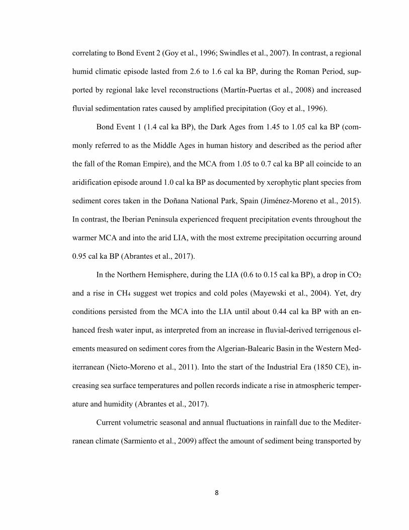
correlating to Bond Event 2 (Goy et al., 1996; Swindles et al., 2007). In contrast, a regional

humid climatic episode lasted from 2.6 to 1.6 cal ka BP, during the Roman Period, sup-

ported by regional lake level reconstructions (Martín-Puertas et al., 2008) and increased

fluvial sedimentation rates caused by amplified precipitation (Goy et al., 1996).

Bond Event 1 (1.4 cal ka BP), the Dark Ages from 1.45 to 1.05 cal ka BP (com-

monly referred to as the Middle Ages in human history and described as the period after

the fall of the Roman Empire), and the MCA from 1.05 to 0.7 cal ka BP all coincide to an

aridification episode around 1.0 cal ka BP as documented by xerophytic plant species from

sediment cores taken in the Doñana National Park, Spain (Jiménez-Moreno et al., 2015).

In contrast, the Iberian Peninsula experienced frequent precipitation events throughout the

warmer MCA and into the arid LIA, with the most extreme precipitation occurring around

0.95 cal ka BP (Abrantes et al., 2017).

In the Northern Hemisphere, during the LIA (0.6 to 0.15 cal ka BP), a drop in CO2

and a rise in CH4 suggest wet tropics and cold poles (Mayewski et al., 2004). Yet, dry

conditions persisted from the MCA into the LIA until about 0.44 cal ka BP with an en-

hanced fresh water input, as interpreted from an increase in fluvial-derived terrigenous el-

ements measured on sediment cores from the Algerian-Balearic Basin in the Western Med-

iterranean (Nieto-Moreno et al., 2011). Into the start of the Industrial Era (1850 CE), in-

creasing sea surface temperatures and pollen records indicate a rise in atmospheric temper-

ature and humidity (Abrantes et al., 2017).

Current volumetric seasonal and annual fluctuations in rainfall due to the Mediter-

ranean climate (Sarmiento et al., 2009) affect the amount of sediment being transported by

9  

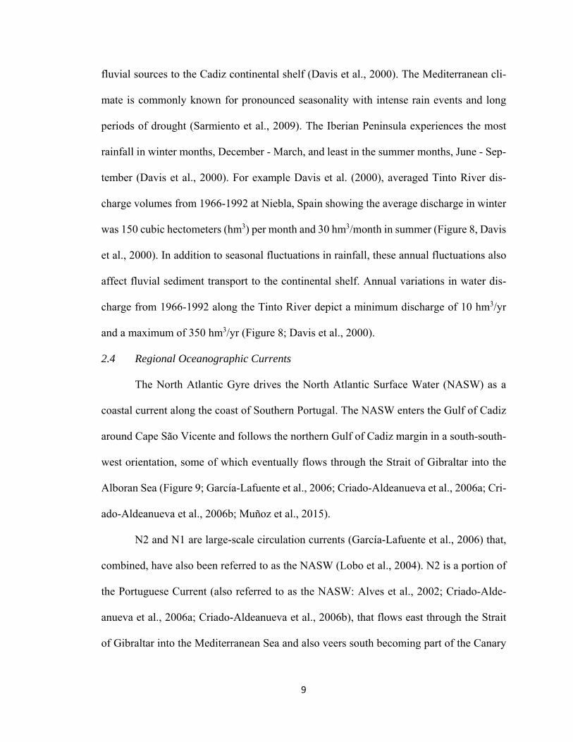
fluvial sources to the Cadiz continental shelf (Davis et al., 2000). The Mediterranean cli-

mate is commonly known for pronounced seasonality with intense rain events and long

periods of drought (Sarmiento et al., 2009). The Iberian Peninsula experiences the most

rainfall in winter months, December - March, and least in the summer months, June - Sep-

tember (Davis et al., 2000). For example Davis et al. (2000), averaged Tinto River dis-

charge volumes from 1966-1992 at Niebla, Spain showing the average discharge in winter

was 150 cubic hectometers (hm3) per month and 30 hm3/month in summer (Figure 8, Davis

et al., 2000). In addition to seasonal fluctuations in rainfall, these annual fluctuations also

affect fluvial sediment transport to the continental shelf. Annual variations in water dis-

charge from 1966-1992 along the Tinto River depict a minimum discharge of 10 hm3/yr

and a maximum of 350 hm3/yr (Figure 8; Davis et al., 2000).

2.4 Regional Oceanographic Currents

The North Atlantic Gyre drives the North Atlantic Surface Water (NASW) as a

coastal current along the coast of Southern Portugal. The NASW enters the Gulf of Cadiz

around Cape São Vicente and follows the northern Gulf of Cadiz margin in a south-south-

west orientation, some of which eventually flows through the Strait of Gibraltar into the

Alboran Sea (Figure 9; García-Lafuente et al., 2006; Criado-Aldeanueva et al., 2006a; Cri-

ado-Aldeanueva et al., 2006b; Muñoz et al., 2015).

N2 and N1 are large-scale circulation currents (García-Lafuente et al., 2006) that,

combined, have also been referred to as the NASW (Lobo et al., 2004). N2 is a portion of

the Portuguese Current (also referred to as the NASW: Alves et al., 2002; Criado-Alde-

anueva et al., 2006a; Criado-Aldeanueva et al., 2006b), that flows east through the Strait

of Gibraltar into the Mediterranean Sea and also veers south becoming part of the Canary

10  

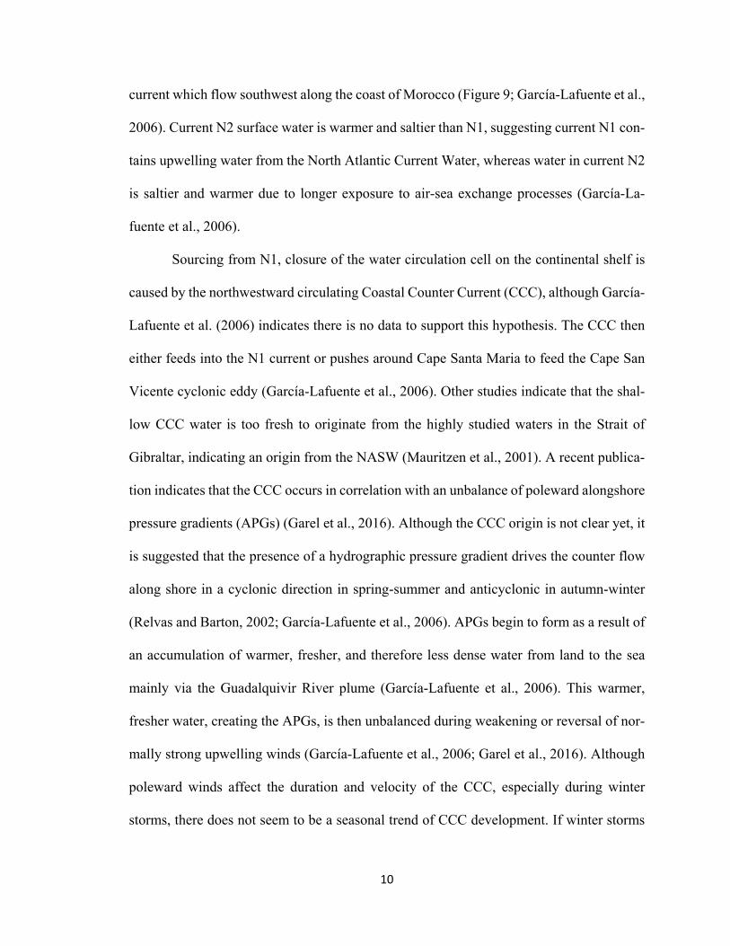
current which flow southwest along the coast of Morocco (Figure 9; García-Lafuente et al.,

2006). Current N2 surface water is warmer and saltier than N1, suggesting current N1 con-

tains upwelling water from the North Atlantic Current Water, whereas water in current N2

is saltier and warmer due to longer exposure to air-sea exchange processes (García-La-

fuente et al., 2006).

Sourcing from N1, closure of the water circulation cell on the continental shelf is

caused by the northwestward circulating Coastal Counter Current (CCC), although García-

Lafuente et al. (2006) indicates there is no data to support this hypothesis. The CCC then

either feeds into the N1 current or pushes around Cape Santa Maria to feed the Cape San

Vicente cyclonic eddy (García-Lafuente et al., 2006). Other studies indicate that the shal-

low CCC water is too fresh to originate from the highly studied waters in the Strait of

Gibraltar, indicating an origin from the NASW (Mauritzen et al., 2001). A recent publica-

tion indicates that the CCC occurs in correlation with an unbalance of poleward alongshore

pressure gradients (APGs) (Garel et al., 2016). Although the CCC origin is not clear yet, it

is suggested that the presence of a hydrographic pressure gradient drives the counter flow

along shore in a cyclonic direction in spring-summer and anticyclonic in autumn-winter

(Relvas and Barton, 2002; García-Lafuente et al., 2006). APGs begin to form as a result of

an accumulation of warmer, fresher, and therefore less dense water from land to the sea

mainly via the Guadalquivir River plume (García-Lafuente et al., 2006). This warmer,

fresher water, creating the APGs, is then unbalanced during weakening or reversal of nor-

mally strong upwelling winds (García-Lafuente et al., 2006; Garel et al., 2016). Although

poleward winds affect the duration and velocity of the CCC, especially during winter

storms, there does not seem to be a seasonal trend of CCC development. If winter storms

11  

were overlooked, the number of times a CCC occurs would be largest in summer. These

inconsistencies indicates the CCC occurs about 40% of the time in a week span (Garel et

al., 2016).

Many publications discuss the mixing of the NASW current and the Mediterranean

Outflow Water (MOW) in the Gulf of Cadiz. It is important to note that this research in the

Gulf of Cadiz however occurred at water depths greater than 200 meters (Baringer and

Price, 1999; Cherubin et al., 2000; Hanquiez et al., 2007; Mulder et al., 2013).

2.5 Fluvial Sources – Characterization and Geologic Foundation

This study focuses on four of seven rivers, Guadalquivir River, Tinto-Odiel Estu-

ary, Piedras River, and Guadiana River, which source fine-grained material to the shelf,

forming MDCs (Figure 1). Contradictory to a normal estuarine behavior, which leads to

sediment trapping inside the estuary, the highly polluted Tinto-Odiel Estuary transports

sediment to the Gulf of Cadiz, evident by heavy metal distribution on the shelf (Ruiz et al.,

2014; Hanebuth et al., 2018).

The Guadalquivir River flows through the Guadalquivir Basin which is part of the

Neogene Basins in the Betic Cordillera (Figure 10; Sanz de Galdeano and Vera, 1992).

From 23 to 5.3 million yrs ago, the basin was submerged and subject to marine deposition

(Sanz de Galdeano and Vera, 1992), under variable subsidence rates and high sediment

supply (Hernández-Molina et al., 2000). The Guadalquivir River watershed expands

57,000 km2 and contains a mean annual discharge rate of 160 m3/s according to Van Geen

et al. (1997). Other sources indicate the discharge rate can exceed 5,000 m3/s in winter

months, especially January to February (Rodríguez-Ramírez et al., 2016). The freshwater

12  

discharge of the Guadalquivir River has a high mean sediment suspended load of 771 mg/L,

seasonally with a minimum of 247 mg/L and maximum of 3,172 mg/L (Ruiz et al., 2013).

Tinto and Odiel Rivers meet within the Guadalquivir Basin to flow together into

the Gulf of Cadiz, but they both originate from the South Portuguese Zone of the Iberian

Massif (Onézime et al., 2002). Within this zone, the Tinto and Odiel Rivers flow through

the Iberian Pyrite Belt (IPB) composed of three lithological groups: (1) the Phyllite-Quartz-

ite Group (2) Volcano-Sedimentary Complex (Volcanogenic Massive Sulfide ore deposit

belt), and (3) the Culm Group from the Upper Devonian to Upper Carboniferous (Figure

10; Barrie and Hannington, 1999; Onézime et al., 2002; Onézime et al., 2003; Sarmiento

et al., 2009). The Phyllite-Quartzite Group consists of a thick sequence of shales and sand-

stones (Sarmiento et al., 2009). The Volcano-Sedimentary Complex consists of an equal

distribution of siliciclastic interstratified shales with felsic and mafic volcanic rocks (Sar-

miento et al., 2009; Barrie and Hannington, 1999). The Culm Group is composed of shales,

sandstones and conglomerates (Sarmiento et al., 2009). Mining activities in the IPB date

back to the third millennium BC with metallurgical production of copper (Nocete et al.,

2005; Hanebuth et al., 2018) causing the fluvial waters to be highly acidic from the oxida-

tion of large quantities of sulfide-rich minerals (Sarmiento et al., 2009; Cáceres et al.,

2013).

The Tinto and Odiel Rivers have seasonally and annually variable water discharge

patterns (Figure 8; Sarmiento et al., 2009; Davis et al., 2000). The Iberian Peninsula expe-

riences the most rainfall in winter months, December to March with 150 hm3, and least in

the summer months, June to September with 30 hm3 from 1966-1992 (Figure 8, Davis et

al., 2000). The 3,400 km2 Tinto-Odiel River watershed contains a mean annual discharge

13  

rate of 20 m3/s (Van Geen et al., 1997) and an estimated annual flow of 500 hm3/yr (Sar-

miento et al., 2009).

Similar to the Tinto and Odiel Rivers, the much smaller Piedras River also origi-

nates from the South Portuguese Zone of the Iberian Massif (Onézime et al., 2002) and

flows through the Guadalquivir Basin just before entering the Gulf of Cadiz. The Piedras

River watershed expands 250 km2 and is thus more than thirteen times smaller than the

Tinto-Odiel system (Borrego et al., 1993). Water and suspended load discharge rates for

the Tinto-Odiel and Piedras Rivers are unavailable.

The Guadiana River also originates from the South Portuguese Zone of the Iberian

Massif and flows through the IPB (Figure 10; Sarmiento et al., 2009; Onézime et al., 2002;

Onézime et al., 2003), encompassing a 67,000 km2 basin with a mean annual discharge of

80 m3/s (Van Geen et al., 1997). The volume estimates for suspended sediment load (0.576

hm3/yr) and bedload (0.44 hm3/yr) were averaged between 1946 and 1990 (Morales, 1997).

Anthropogenic land use has caused chronological markers to occur as early as the

Bronze Age in the Alboran Basin and Zoñar Lake in Spain, near to this study area (Figure

11; Martín-Puertas et al., 2010). Lead (Pb) enrichment depicts peaks during enhanced min-

ing and smelting activity initially caused from Iberian mining beginning during Phoenician

Era (3.0 to 2.6 cal ka BP), at large scale during the Roman Empire (2.05 to 1.75 cal ka BP),

to a very subtle amount during Medieval Times (0.95 to 0.75 cal ka BP) and at unprece-

dented high levels during the Industrial Era (0.2 cal ka BP to present) (Figure 11; Martín-

Puertas et al., 2010). Hanebuth et al. (2018) recently correlated heavy metal contamination

signatures on the continental shelf in this study area with mining major activities during

the Roman Period and the Industrial Era.

14  

2.6 Shelf Characteristics and Stratigraphy

Under the continental shelf, the Triassic Allochthonous Unit has been undergoing

extension in the NW-SE orientation due to compression in the NE-SW orientation, perpen-

dicular to the shelf (Fernández-Puga et al., 2007; Medialdea et al., 2009). The under-com-

pacted shale and evaporitic material have since migrated through NW-SE extension faults

promoting diapiric processes since early Miocene (Fernández-Puga et al., 2007; Medialdea

et al., 2009). The migration of evaporitic units has caused subsidence of overlying units by

shelf extension (Nelson et al., 1999; Fernández-Puga et al., 2007; Medialdea et al., 2009).

The morpho-dynamic features of the shelf between the Tinto-Odiel Estuary and

Guadalquivir River area are characterized by subsidence and a shelf gradient gentler than

0.2° (Lobo et al., 2002). In contrast, off the Guadalquivir River mouth, the shelf is charac-

terized by uplifting due to diapiric-like structures (Lobo et al., 2002).

The muddy prodelta off of the Guadalquivir River has been characterized with five

distinct units (Fernández-Salas et al., 2003). The oldest unit, identified as transgressive

deposits, shows characteristics of aggradational deposition and discontinuous internal re-

flectors (Fernández-Salas et al., 2003). The four overlying units are characterized by

prodeltaic deposits portraying two alternating sequences of progradational growth overlain

by aggradational subunits (Figure 6; Lobo et al., 2005). The aggradational deposits contain

sub-parallel internal reflectors while the progradational deposits contain downlapping in-

ternal reflectors (Figure 6; Lobo et al., 2004; Fernández-Salas et al., 2003).

Sedimentation rates for this region of the Gulf of Cadiz are limited to specific lo-

cations and by general age coverage. Nelson et al. (1999) calculated sedimentation rates

for the entire shelf from the Guadiana River to the Bay of Cadiz (Figure 1) using eustatic

15  

sea level curves and sediment isopach thickness. Highest rates were found closest to the

Guadalquivir River at 234 cm ka-1 for the past 6000 yrs. One location close to shelf edge,

between the Tinto-Odiel Estuary and Guadalquivir River showed a sedimentation rate of

22.6 cm ka-1 for the past 9000 yrs and 110 to 160 cm ka-1 for the recent 100 yrs (Nelson et

al., 1999). Sedimentation rates based on sediment cores with good age resolution were

collected close to the Guadiana River (Mendes et al., 2010, 2012) with oldest sedimentation

rates averaging 10 cm ka-1 from 10.2 to 4.3 cal ka BP (mud body and transgressive bulge:

Mendes et al., 2012). Younger sedimentation rates near the Guadiana River were 52 cm

ka-1 from 5.2 to 3.8 cal ka BP, slightly increasing to 59 cm ka-1 from 3.8 to 1.3 cal ka BP,

then more than doubling to 128 cm ka-1 from 1.3 to 0.68 cal ka BP (mud body and prodel-

taic wedge: Mendes et al., 2010, 2012).

16  

3.0 Objectives and Research Questions

To focus this thesis, two major objectives with related questions were identified.

Due to substantial variety of data sets, Table 1 depicts why each methodological approach

and associated data set is to be used for generating answers on the following two objectives.

The third objective, which was originally part of the thesis proposal, relating to mecha-

nisms controlling sediment accumulation within MDCs was removed due to a too limited

data set and time constraints on thesis completion.

3.1 Chrono- and Lithostratigraphy of Mud Depocenters

This objective aims at determining the geometric formation of Holocene MDCs

using seismo-acoustic echosounder and boomer data sets. Previous studies of seismo-

acoustic datasets in this region showed that there is probably a larger sediment unit above

the mfs increasing in landward direction near the Guadalquivir River, but gas masking

obscures data (Fernández-Salas et al., 2003; Lobo et al., 2005). Are those stratigraphic units

partly aggradational or are there definite progradational trends? Older investigations in the

region determined separate aggradational and progradational units (Lobo et al., 2005: Her-

nández-Molina et al., 1994). Is a prodelta facies found in all of the near-shore profiles?

This will be determined by studying the internal geometries of the units through seismo-

acoustic profiles. Seismo-acoustic profiles along with magnetic susceptibility scans and

XRF scanner intensities, will be used to correlate stratigraphic units. Lithology descrip-

tions, radiography images, and high-resolution core images will be used for detailed facies

determination. An attempt at sediment source differentiation will be conducted using

17  

magnetic susceptibility scans, and XRF scanner element intensities combined with XRF

powder element concentrations. Carbonate content, total organic content (TOC), bulk den-

sity and porosity data will help to distinguish unit boundaries within MDCs. To acquire an

age control on the stratigraphy of the MDCs, 14C dates and 210Pb profiles will be used.

3.2 Budget Calculation of Mud Depocenters

Once correlation of stratigraphic units between cores has been completed using

XRF scanner and magnetic susceptibility data, the volume of the Holocene accumulated

sediment and distinguishable sub-units of the study area will be determined. By determin-

ing an age structure of the depocenter using 14C dates and 210Pb profiles and combining it

with grain density data, accumulation rates will be calculated. Once volumetric and mass

characteristics of the MDCs are determined, combining them with rates that fluvial sources

provide sediment to the shelf can determine a full retention budget (Oberle et al., 2014).

The volume and mass of the MDCs, with the carbonate content and TOC, a carbon budget

can separately be calculated to further understand the retention of carbon in the MDCs.

Does the part of the Holocene mudbelt, located closest to the mouth of the Guadalquivir

River (assumed as the main sediment supplier), have the highest accumulation rate in the

region, and did the accumulation rates vary through time? Changes in accumulation rates

can potentially depict climatic and anthropogenic industrial-related changes.

18  

4.0 Materials and Methods

In March 2015, subbottom echosounder data and sediment cores were collected in

the Gulf of Cádiz during research cruise POS482 CADISED on the German RV POSEI-

DON near southern Portugal and southwestern Spain. One of the main goals of this cruise,

involving all collaborative partners, has been to develop a robust facies framework of the

sedimentary deposits in Holocene MDCs. This framework will then support various re-

search oceanography-, climate-, and stratigraphy-related targets.

Subbottom data (2,040 km) were acquired using a 4 kHz parametric source that

provided ~20 m subsurface penetration with an INNOMAR subbottom echosounder. The

hull-mounted ELAC Nautik SeaBeam 3050 multibeam echosounder operated at 50 kHz

collecting bathymetric, backscatter and occasionally water column imaging data (Hanebuth

et al., 2014: Cruise report POS482).

Gravity cores with up to 6 m penetration were collected in regions where deposits

of fine-grained sediment and mud were of significant thickness. Coincident 1.5-m long

Ruhmor cores were also collected to preserve the uppermost sediment layer. Of the 40

cruise stations completed using varying coring methods, 18 stations are located within the

study area.

Twelve data sets were collected and measured from echosounder data and 18 sedi-

ment cores (Table 3). High-resolution photographic images of halved sediment cores were

taken using a smartCIS 1600 Line Scanner. Lithology of 18 sediment cores was described

by color, grain size, and composition. Magnetic susceptibility and porosity were measured

19  

on 15 cores. Using samples collected from gravity and Ruhmor cores from 11 stations,

porosity and density were calculated by using dry bulk density. Seven gravity cores were

x-ray florescence (XRF) scanned for element intensities, six of which had samples pro-

cesses for x-ray powder element concentration measurement. Total Organic Content

(TOC) and carbonate content (CaCO3) were measured on five representative gravity cores.

Accelerator Mass Spectrometer (AMS) 14C dating were performed for nine representative

gravity cores (19512-3, 19513-3, 19518-3, 19519-3, 19520-3, 19521-3, 19534-3, 19535-3,

and 19538-3: Figure 2). Samples for 210Pb and 137Cs excess profiles were measured from

four and two, respectively, of the nine gravity cores. Radiography images were taken from

Core 19520-3. A complete list of data sets collected is provided in Table 3.

4.1 Seismo-Acoustic Data

IHS Kingdom Software 2015 was used to view pre-processed seismo-acoustic pro-

files to correlate major internal reflectors. In addition to the POS482 seismo-acoustic data,

boomer data collected with a Geopulse from 1992 and 1986 (courtesy of Dr. Lobo), were

used to extend the penetration depth. Grids used for the volumetric calculations and isopach

maps were created by tracing major reflectors in the echosounder profiles and using the

corresponding the age model from coring sites. The “Flex Gridding” algorithm was used

with 0.3 curvature, a 1 minimum smoothness, grid cell size of 100 in the X and Y direction,

and a convex hull extrapolation limit of 0 m. Volumes produced utilize a sound velocity of

1500 m s-1. The volume of material between two grid levels was determined by calculating

the net volume using duel structure grids. Output parameters were set to the grid with the

smallest surface area with an inverse distance to power weight of 2. These profiles were

utilized to understand boundaries between MDC facies.

20  

4.2 Multi-Sensor Core Logger (MSCL) Data

Sediment core sections were scanned through a multi-sensor core logger (MSCL),

prior to opening. Although additional analysis was conducted, this study utilized only mag-

netic susceptibility and porosity values. Magnetic susceptibility intensity values were used

for in-detail correlation of cores with one another to determine source differentiation, and

depict changes in MDC depositional centers.

4.3 Sediment Properties and Budget Calculation

The following calculations were conducted to develop a sediment budget estimate

using the sediment volume and mass through various time intervals, thereby depicting tem-

poral changes of the MDCs.

Sediment samples were collected using 10 mL syringes at depth intervals of five to

fifteen cm in each core. Before drying material, the exact sediment volume (VT) of sedi-

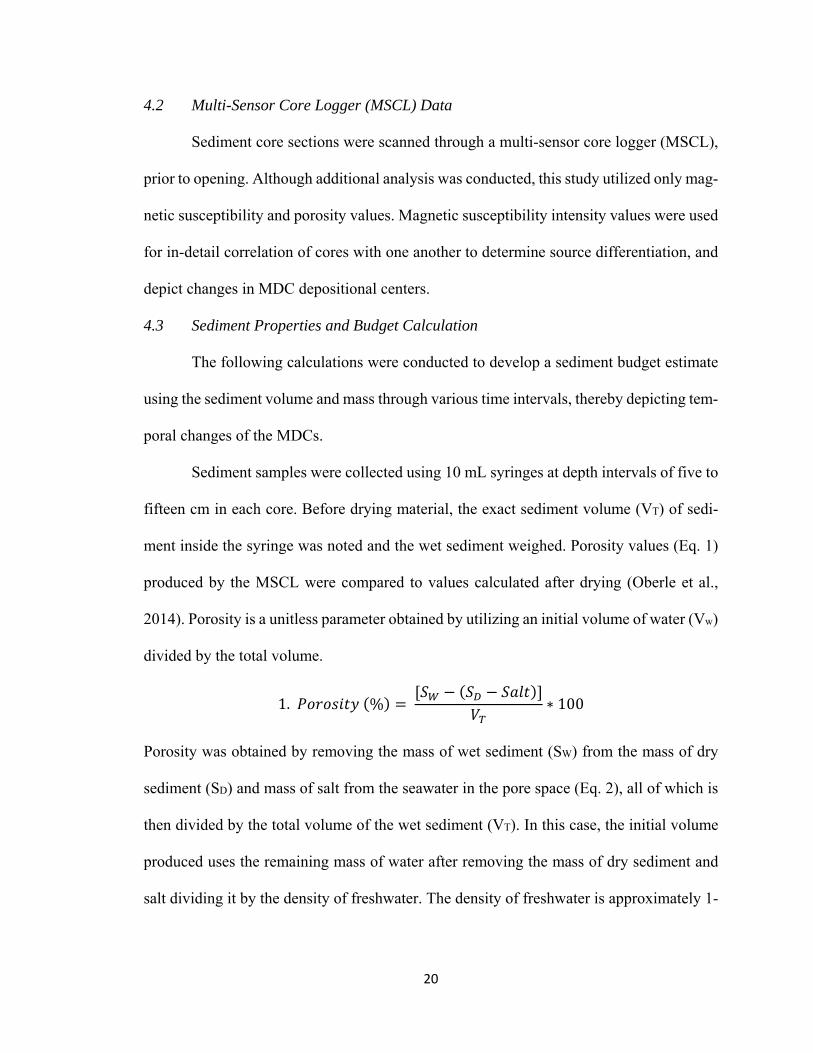
ment inside the syringe was noted and the wet sediment weighed. Porosity values (Eq. 1)

produced by the MSCL were compared to values calculated after drying (Oberle et al.,

2014). Porosity is a unitless parameter obtained by utilizing an initial volume of water (Vw)

divided by the total volume.

1. % ∗ 100

Porosity was obtained by removing the mass of wet sediment (SW) from the mass of dry

sediment (SD) and mass of salt from the seawater in the pore space (Eq. 2), all of which is

then divided by the total volume of the wet sediment (VT). In this case, the initial volume

produced uses the remaining mass of water after removing the mass of dry sediment and

salt dividing it by the density of freshwater. The density of freshwater is approximately 1-

21  

g mL-1, therefore the remaining mass of the water in grams is equal to the initial volume of

water in milliliters.

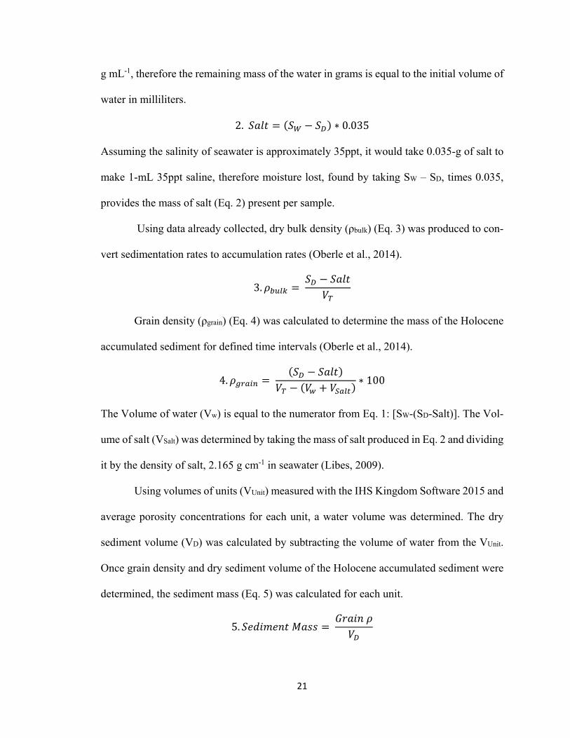
2. ∗ 0.035

Assuming the salinity of seawater is approximately 35ppt, it would take 0.035-g of salt to

make 1-mL 35ppt saline, therefore moisture lost, found by taking SW – SD, times 0.035,

provides the mass of salt (Eq. 2) present per sample.

Using data already collected, dry bulk density (ρbulk) (Eq. 3) was produced to con-

vert sedimentation rates to accumulation rates (Oberle et al., 2014).

3.

Grain density (ρgrain) (Eq. 4) was calculated to determine the mass of the Holocene

accumulated sediment for defined time intervals (Oberle et al., 2014).

4. ∗ 100

The Volume of water (Vw) is equal to the numerator from Eq. 1: [SW-(SD-Salt)]. The Vol-

ume of salt (VSalt) was determined by taking the mass of salt produced in Eq. 2 and dividing

it by the density of salt, 2.165 g cm-1 in seawater (Libes, 2009).

Using volumes of units (VUnit) measured with the IHS Kingdom Software 2015 and

average porosity concentrations for each unit, a water volume was determined. The dry

sediment volume (VD) was calculated by subtracting the volume of water from the VUnit.

Once grain density and dry sediment volume of the Holocene accumulated sediment were

determined, the sediment mass (Eq. 5) was calculated for each unit.

5.

22  

Porosity and dry bulk density measurements supported the identification and characteriza-

tion of sedimentary facies and their stratigraphic boundaries. For instance, an increasing

porosity indicates, wider pore space; taking compaction into consideration, porosity should

decrease with increasing depth in core. Variations in grain density and dry bulk density

indicate sediment compositional changes within or between facies.

4.4 X-ray Fluorescence Element Scanning

Using the MSCL data and seismo-acoustic profiles, 10 representative cores were

chosen for the non-destructive, high-resolution X-ray fluorescence (XRF) scanner. The ar-

chive halves of these 10 cores were analyzed at MARUM through a XRF AVAATECH

(Serial No. 2) using a Canberra X-PIPS Silicon Drift Detector (SDD; Model SXD 15C-

150-500) with an Oxford Instruments XTF5011 X-Ray Tube 93057. Sections containing

sharp shell fragments or sandy sediment cannot be scanned. The intensities (in counts) of

light elements were measured in 1 cm intervals at 10kV with a 0.2 milliampere (mA) cur-

rent for 15 sec; heavy elements at 30kV with a 1.0 mA current for 15 sec. After quality

checks of the processed data, not all element intensities are considered reliable due to low

concentrations, limitation of the sensor sensitivity, or contamination by elements emitted

by the XRF scanner components.

4.4.1 Element Intensity Ratios

Since element intensities do not depict true element concentrations, the ratio be-

tween two elements is used as a proxy to detect an environmental change. The ratios were

then normalized to keep scales consistent by taking the natural logarithm. Element intensity

ratios are often used for paleoceanographic and paleo-environmental reconstructions. Ln

23  

Ca/Fe ratios and ln Ti/Zr were also used for transferring age tie points between the indi-

vidual sediment cores, since elements show comparable and high intensities.

The weathering-resistant Zirconium (Zr) is commonly associated with coarser-

grained minerals. Titanium (Ti) is associated with minerals that are more easily weathered

than minerals with Zr, thus Ti is found in the finer sediment fraction. As this ratio increases,

the grain size becomes finer. To calibrate this proxy, grain size measurements should have

been conducted at CCU with a Laser diffraction particle size analyzer. Due to timing con-

straints and lasting technical issues with maintenance of both available machines, grain

size measurements were not included in this study and will be performed in near future.

The ln Ca/Fe ratio depicts variations in the relative amount of marine sourced (=

biogenic carbonate) to terrigenous (= siliciclastic) material (assuming iron (Fe) is entirely

of terrestrial origin; Hanebuth et al., 2015b). Previous studies indicated Fe and Ti are

closely related to each other in the terrigenous fraction, yet Fe can be prone to secondary

remobilization after deposition through diagenesis but Ti is considered chemically stable

in its hosting minerals (Richter et al., 2006; Tjallingii et al., 2010). Fe is mainly present in

clay minerals, pyrite, and various iron minerals derived from continental soils and mag-

matic rocks. Fe is also present in organic material. Since the measured TOC values range

from 0.4 – 0.9% (Table 4), only a negligible fraction of Fe may be marine sourced, but it

is not enough to disprove this proxy for marine sourcing vs. terrigenous. Ln Fe/Ti was

plotted to verify if background levels of both elements (preanthropogenic contamination)

did not show significant fluctuations, i.e., to prove that Fe was not affected by secondary

ion migration, allowing Fe to be used as an indicator for primary terrigenous supply (Figure

12).

24  

4.4.2 X-ray Fluorescence Powder Element Measurement

To convert the intensity curves of single elements of interest into true element con-

centration records, eight to fifteen samples per core were measured for element concentra-

tions using a SPECTROXEPOS (methods Opti2 and 2016-CaCO3). The selected samples

were collectively measured for TC and TOC using a LECO CS-200 carbon and sulfur in-

frared detection analyzer.

4.5 14C Dating

Eighteen depths in cores, selected by reviewing core descriptions and seismo-

acoustic profiles, were dated using AMS-14C precision dating. If no larger and in-situ pre-

served bivalves or Turritella-like gastropods existed at these precise depths, foraminifera

were carefully picked. Benthic foraminifera were targeted for 14C samples, but to acquire

at least 20 mg per sample, all freshly preserved carbonate material had to be selected in

some instances. All deteriorating, stained, broken or potentially remobilized material was

avoided to not contaminate samples with old material. Of the eighteen samples, twelve

were composed of foraminifera and six of in-situ bivalves or gastropods. Foraminifera

samples were sieved at 63 µm to remove the mud fraction. Each sample took approximately

40 hours to complete. The samples were shipped to Poznan Radiocarbon Lab in Poland.

Two benthic foraminifera samples were collected by Dr. Susana Lebreiro (IGME) and

measured at the National Accelerator Center at the University of Sevilla, Spain. Once re-

ceived, the conventional ages were put into version 7.10 of the CALIB Radiocarbon Cali-

bration Program to calibrate samples to the carbon changes in the atmosphere through time

using data set ‘marine13.14c’ (Stuiver and Reimer, 1993; Reimer et al. 2013). Marine 14C

dated samples cannot be compared to terrestrial samples without accounting for the age of

25  

the seawater, i.e., the reservoir age. To keep ages consistent, the global average reservoir

age of 406 yrs, was removed from 14C dates. Although samples were collected from a shal-

lower ocean system, no local reservoir was used to modify the ages, due to the possible

existence of an older carbon signature by deeper upwelled water. The calibrated (cal) 14C

ages are given in ‘before present’ (BP); the ‘present’ being 1 January 1950 (Currie, 2004).

These dates helped to establish a shelf-wide age framework for the MDCs and to calculate

time- and location-specific sedimentation and accumulation rates.

4.6 210Pb and 137Cs Dating

Young ages from the first set of 14C samples prompted the use of 210Pb and 137Cs

dating techniques on Cores 19520-3 every 10 cm for the first 150 cm (closest to the Gua-

dalquivir River mouth), 19512-3 every 10 cm for 100 cm (center of study area), 19534-3

with 24 samples for 70 cm (closest to the Tinto-Odiel Rivers mouth), and 19535-3 every

10 cm for 100 cm (near to the Tinto-Odiel Rivers mouth). Ages for 19520-3 and 19534-3

were measured by the Laqimar Laboratory in Sao Paulo, Brazil (Dr. Paulo Alves Ferreira).

Measurements for 19512-3 and 19535-3 were measured in the USGS facility in Santa Cruz

(Dr. Ferdinand Oberle). Since the study area is heavily influenced by sediment supply from

the continent and oceanographic currents, the also measured 137Cs profiles were reviewed

critically and decidedly not used for the age model. 210Pb profiles were generated using

two calculation models: Constant Rate of Supply (CRS) and Constant Initial Concentration

(CIC). Since XRF element intensity curves and XRF powder concentrations showed the

sediment concentration did not remain constant, the results provided by the CRS model

were used, which in general seems to describe processes in shallow waters more appropri-

ately (Appleby and Oldfield 1978; personal communication Dr. P. Alves, Dr. F. Oberle).

26  

CRS assumes the flux of unsupported 210Pb deposited at a constant rate. The ages produced

by 210Pb dating were also used to understand when heavy metal contamination in the Gulf

of Cadiz, Spain changed through industrial periods (Hanebuth et al., 2018). 210Pb sourced

ages are given in ‘common era’ (CE). Table 1 depicts a summary of which method was

used for to address each objective of this thesis.

4.7 High-Resolution Core Imaging

All cores were photographed to produce high-resolution images in millimeter scale.

Radiographies were taken from Core 19520-3, located near the mouth of the Guadalquivir

River, to visualize the millimeter-scale resolution depicting the succession of flood layers.

Radiography images provide internal detail of sediment texture and structure. The high-

resolution core images and radiography images assist in distinguishing facies boundaries.

27  

5.0 Critical Evaluation of Stratigraphic Age Model and Material Budgets

5.1 Calculation of Sedimentation Rates

Element intensities were converted into ratios to correlate cores stratigraphically

and depict changes in sediment deposition by core location. The natural log of these ratios

(ln(Ca/Fe), ln(Ti/Zr), ln(Zn/Al), and ln(Pb/Al)) in each data set were used to normalize

figure scales to make visual correlation between cores accurate. An example of this inter-

pretive method depicts ln (Ca/Fe) from Cores 19538-3, 19513-3, and 19518-3 (Figure 13).

Zn and Pb are known sources of anthropogenic pollution in the Gulf of Cadiz (Ruiz, et al.,

2014; see Hanebuth et al., 2018 for more references). These metals were normalized to

aluminum (Al) since Al is assumed to be entirely sourced from the clay fraction (Delgado

et al., 2012) of the terrigenous supply (Martín-Puertas, et al., 2010; Pipper and Perkins,

2004; Nieto-Moreno et al., 2011) and used as a representative of fines in a grain-size dis-

tribution (Hanebuth et al., 2018). Ln Ti/Zr ratio was explained in section 5.4.1 Element

Intensity Ratio. Ln Ti/Al ratio was taken to depict Ti and Al are present in the material at

an approximate 1:1 ratio, making them interchangeable (Figure 14). Ti is also known to be

mainly sourced from terrigenous material (Richter et al., 2006).

The element ratios (ln Ca/Fe, ln Ti/Zr, ln Zn/Al, and ln Pb/Al), and the magnetic

susceptibility curves were also used for a robust inter-core correlation. Nine representative

coring stations were compared in six transects by proximity to shore (Table 2). The three

28  

coring stations most proximal, central, and distal to shore, were compared in three tran-

sects. For example, Sites 19538 (closer to the Tinto-Odial Estuary), 19513, and 19518

(closer to the Guadalquivir River) were compared to each other (Figure 13, locations de-

picted in Figure 2). Sites were also compared from proximal to distal in three transects.

Sites 19534 (closest to the Tinto-Odial Estuary), 19535, 19538 were compared to each

other (Figure 15, locations depicted in Figure 2). Once the correlation model was complete,

the depths at which each correlation line landed were compiled by depth on a core transect

(Figures 16 and 17). This stratigraphic model was used to transfer absolute ages received

from 210Pb profiles (Table 6) and calibrated 14C dates (Table 5). Due to the coarse material,

some of the oldest core sections were could not be XRF scanned. Therefore, some of the

oldest ages were transferred from core to core by tracing major reflectors in seismo-acous-

tic profiles. This framework allowed for detailed sedimentation and accumulation rates to

be determined.

Although this approach led to the calculation of detailed sedimentation and accu-

mulation rates, there is error to be considered. There are limitations to 14C dating and hu-

man error associated with picking material. Bioturbation and lateral transport can cause

younger material to be located deeper in the sediment succession than its natural deposi-

tional depth or older material to be pulled to younger depths. While benthic foraminifera

are being picked with great care, older material can accidentally be chosen causing the age

to be older than the sample depth. The gravity coring method can also cause compression

or expansion of layers, thereby altering the true accumulation rates artificially. Gravity

coring can also cause a loss of material of the uppermost 0-15 cm. These reasons alone

give all ages a conservative error of ± 15 cm. By using the ratio correlation method, an

29  

additional error is given to those ages depending on how easily or how far ages transpose

vertically since this method identifies peaks and trends in the magnetic susceptibility and

XRF element distribution curves. Since it is not always straight-forward to patch the related

peaks from core to core additional error of ± 1 to 20 cm can be added. For ages transferred

by following major reflectors on seismo-acoustic profiles the maximum error was given to

the age, thus far (± 35 cm), ± an additional 10 to 40 cm due to limit in vertical echosounding

resolution. These errors are considered when calculating average sedimentation rates for

each core (Figures 18, 19, and 20).

5.2 Calculation of Material Budgets

To generate volumetric and mass budgets of the Holocene accumulated sediment,

porosity and grain density was first calculate by the methods listed in Section 5.3.3 Sedi-

ment Sample Properties. Based on coring methods and core penetration, more samples

were collected from younger facies than older facies. Instead of using average porosity and

grain density values for all of the samples, values were averaged by facies, F & E (com-

bined), D, C, B, A). Facies determination is based off of lithology description and core

images. Ages bounding facies are sourced from the stratigraphic age model. Three major

time slices were used for volumetric and mass budget calculations: Slice 1 – base of the

MDCs to 2.0 cal ka BP (composed of Facies D, E, and F), Slice 2 – 2.0 to 1.0 cal ka BP

(composed of Facies C), and Slice 3 – 1.0 cal ka BP to present (composed of Facies A and

B). To accurately represent porosity and grain density values in Slice 3, values were aver-

aged from Facies A and B. The same concept was used for Slice 1. This approach for an

accurate representation of vertical changes of sediment properties was also applied for the

TOC and CaCO3 mass calculations.

30  

6.0 Results

6.1 Age framework

Nine sediment cores with 18 calibrated 14C ages span from 8.98 cal ka BP, near the

Tinto-Odiel Estuary (bottom of core 19521-3), to 0.44 cal ka BP off the Guadalquivir River

(bottom of core 19519-3) (Table 5). A resolution of at least an age every millennia was

collected, except for time between 4.35 to 2.70 cal ka BP. Reliable 210Pb ages using model

CRS range from 1950 to 2010 CE off the Guadalquivir River (19520-3) and 1930 to 2000

CE near the Tinto-Odiel Estuary (19534-3) (Table 6). Cores 19512-3 and 19535-3, located

centrally parallel to shore, contain dependable ages ranging from 1930 to 1990 CE.

6.2 Determination and Timing of Sedimentary Facies

While echosounder data depicts qualitative information about the depositional ar-

chitecture of the MDCs, gravity cores provide a laterally scattered but temporally/strati-

graphically higher resolution insight into depositional patterns and facies composition. To-

gether with the sedimentary facies determination, average sedimentation rates are pre-

sented for each facies in the following. For exact and average sedimentation rates for each

site refer to Table 7 and Figures 18, 19, and 20

Using photographic images, lithology descriptions, and element intensity ratios, six

main sedimentary facies were identified (Figure 21). In general, grain size fined up core in

the MDCs (Figure 22). These facies were moderately to highly bioturbated and contained

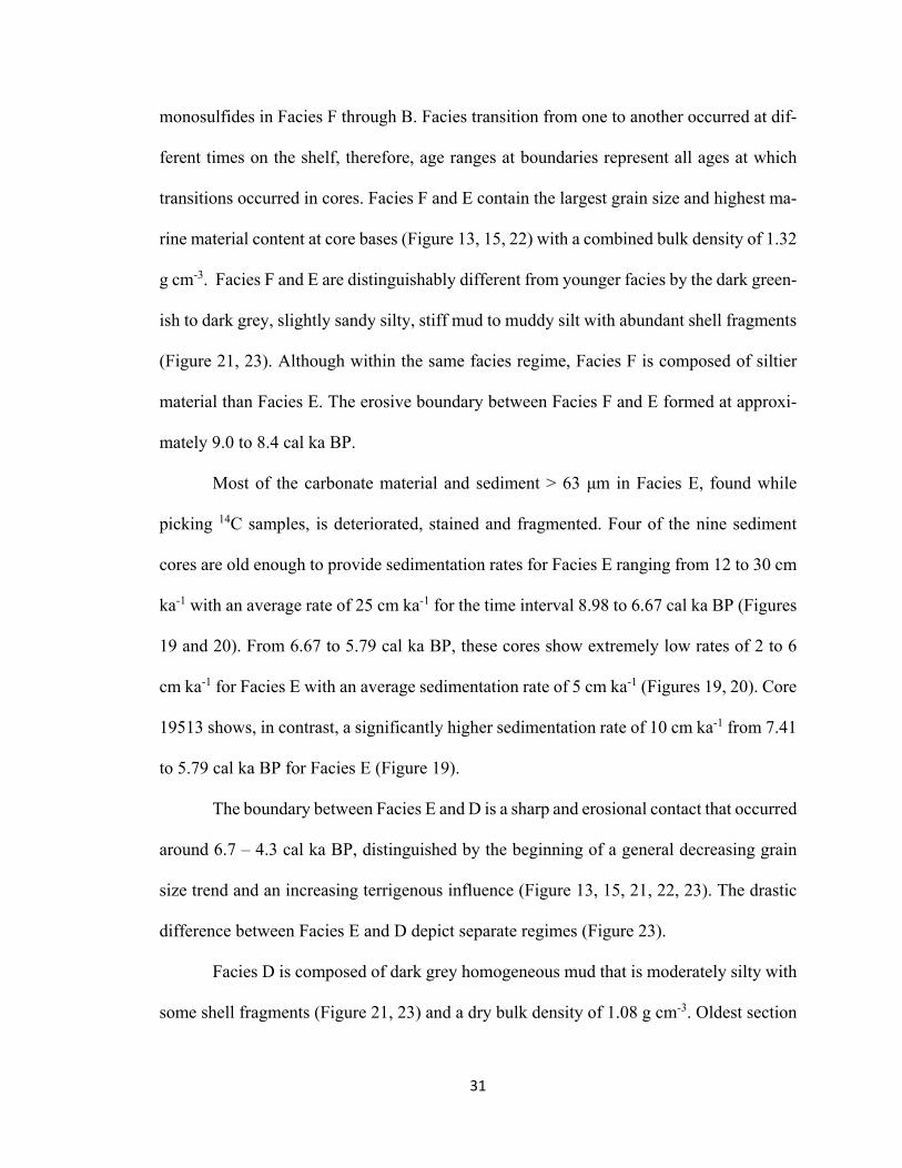
31  

monosulfides in Facies F through B. Facies transition from one to another occurred at dif-

ferent times on the shelf, therefore, age ranges at boundaries represent all ages at which

transitions occurred in cores. Facies F and E contain the largest grain size and highest ma-

rine material content at core bases (Figure 13, 15, 22) with a combined bulk density of 1.32

g cm-3. Facies F and E are distinguishably different from younger facies by the dark green-

ish to dark grey, slightly sandy silty, stiff mud to muddy silt with abundant shell fragments

(Figure 21, 23). Although within the same facies regime, Facies F is composed of siltier

material than Facies E. The erosive boundary between Facies F and E formed at approxi-

mately 9.0 to 8.4 cal ka BP.

Most of the carbonate material and sediment > 63 μm in Facies E, found while

picking 14C samples, is deteriorated, stained and fragmented. Four of the nine sediment

cores are old enough to provide sedimentation rates for Facies E ranging from 12 to 30 cm

ka-1 with an average rate of 25 cm ka-1 for the time interval 8.98 to 6.67 cal ka BP (Figures

19 and 20). From 6.67 to 5.79 cal ka BP, these cores show extremely low rates of 2 to 6

cm ka-1 for Facies E with an average sedimentation rate of 5 cm ka-1 (Figures 19, 20). Core

19513 shows, in contrast, a significantly higher sedimentation rate of 10 cm ka-1 from 7.41

to 5.79 cal ka BP for Facies E (Figure 19).

The boundary between Facies E and D is a sharp and erosional contact that occurred

around 6.7 – 4.3 cal ka BP, distinguished by the beginning of a general decreasing grain

size trend and an increasing terrigenous influence (Figure 13, 15, 21, 22, 23). The drastic

difference between Facies E and D depict separate regimes (Figure 23).

Facies D is composed of dark grey homogeneous mud that is moderately silty with

some shell fragments (Figure 21, 23) and a dry bulk density of 1.08 g cm-3. Oldest section

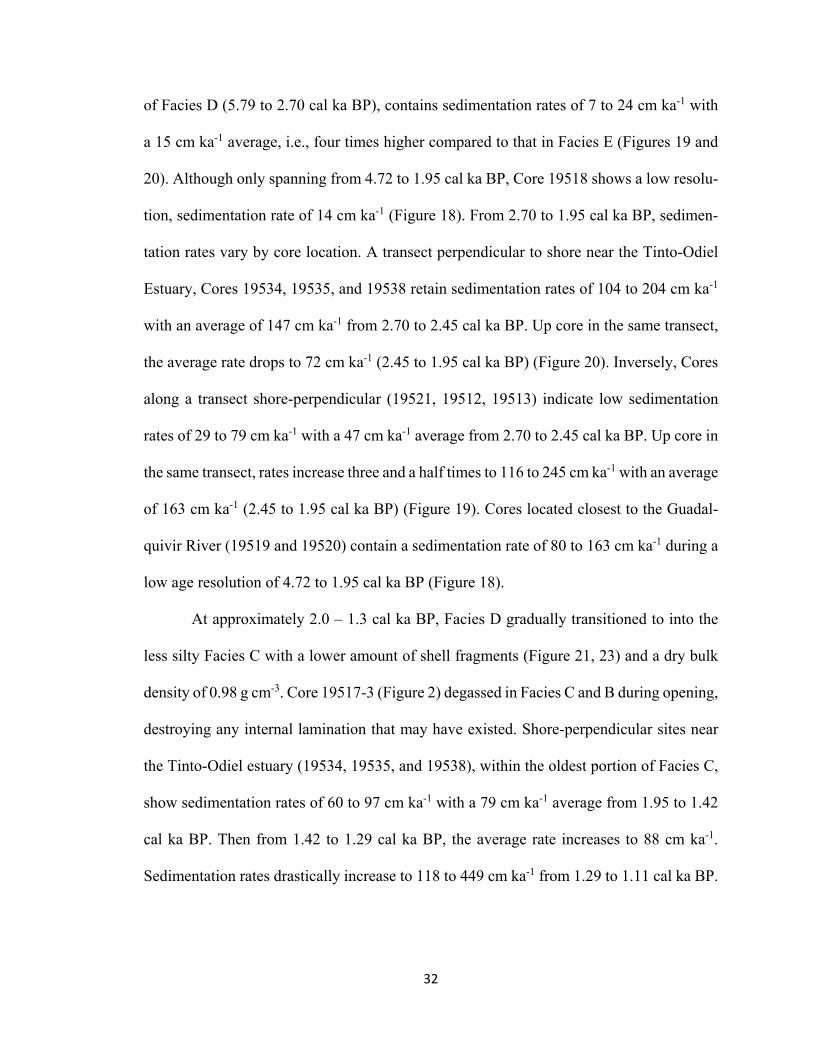
32  

of Facies D (5.79 to 2.70 cal ka BP), contains sedimentation rates of 7 to 24 cm ka-1 with

a 15 cm ka-1 average, i.e., four times higher compared to that in Facies E (Figures 19 and

20). Although only spanning from 4.72 to 1.95 cal ka BP, Core 19518 shows a low resolu-

tion, sedimentation rate of 14 cm ka-1 (Figure 18). From 2.70 to 1.95 cal ka BP, sedimen-

tation rates vary by core location. A transect perpendicular to shore near the Tinto-Odiel

Estuary, Cores 19534, 19535, and 19538 retain sedimentation rates of 104 to 204 cm ka-1

with an average of 147 cm ka-1 from 2.70 to 2.45 cal ka BP. Up core in the same transect,

the average rate drops to 72 cm ka-1 (2.45 to 1.95 cal ka BP) (Figure 20). Inversely, Cores

along a transect shore-perpendicular (19521, 19512, 19513) indicate low sedimentation

rates of 29 to 79 cm ka-1 with a 47 cm ka-1 average from 2.70 to 2.45 cal ka BP. Up core in

the same transect, rates increase three and a half times to 116 to 245 cm ka-1 with an average

of 163 cm ka-1 (2.45 to 1.95 cal ka BP) (Figure 19). Cores located closest to the Guadal-

quivir River (19519 and 19520) contain a sedimentation rate of 80 to 163 cm ka-1 during a

low age resolution of 4.72 to 1.95 cal ka BP (Figure 18).

At approximately 2.0 – 1.3 cal ka BP, Facies D gradually transitioned to into the

less silty Facies C with a lower amount of shell fragments (Figure 21, 23) and a dry bulk

density of 0.98 g cm-3. Core 19517-3 (Figure 2) degassed in Facies C and B during opening,

destroying any internal lamination that may have existed. Shore-perpendicular sites near

the Tinto-Odiel estuary (19534, 19535, and 19538), within the oldest portion of Facies C,

show sedimentation rates of 60 to 97 cm ka-1 with a 79 cm ka-1 average from 1.95 to 1.42

cal ka BP. Then from 1.42 to 1.29 cal ka BP, the average rate increases to 88 cm ka-1.

Sedimentation rates drastically increase to 118 to 449 cm ka-1 from 1.29 to 1.11 cal ka BP.

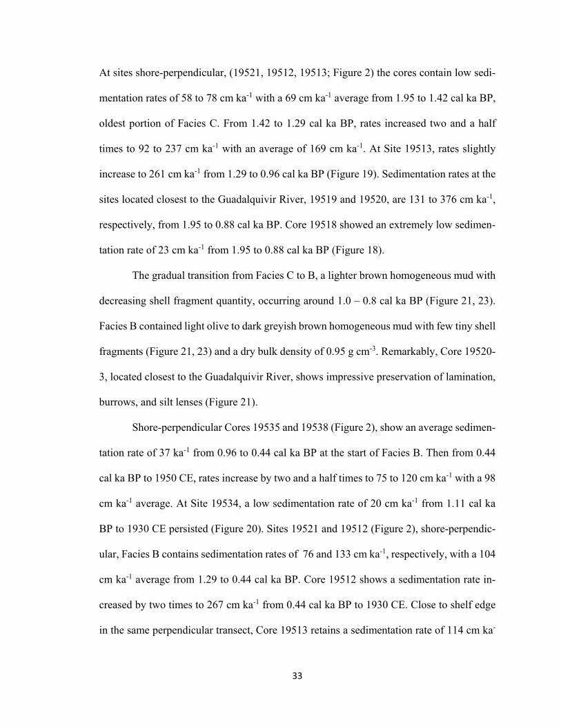
33  

At sites shore-perpendicular, (19521, 19512, 19513; Figure 2) the cores contain low sedi-

mentation rates of 58 to 78 cm ka-1 with a 69 cm ka-1 average from 1.95 to 1.42 cal ka BP,

oldest portion of Facies C. From 1.42 to 1.29 cal ka BP, rates increased two and a half

times to 92 to 237 cm ka-1 with an average of 169 cm ka-1. At Site 19513, rates slightly

increase to 261 cm ka-1 from 1.29 to 0.96 cal ka BP (Figure 19). Sedimentation rates at the

sites located closest to the Guadalquivir River, 19519 and 19520, are 131 to 376 cm ka-1,

respectively, from 1.95 to 0.88 cal ka BP. Core 19518 showed an extremely low sedimen-

tation rate of 23 cm ka-1 from 1.95 to 0.88 cal ka BP (Figure 18).

The gradual transition from Facies C to B, a lighter brown homogeneous mud with

decreasing shell fragment quantity, occurring around 1.0 – 0.8 cal ka BP (Figure 21, 23).

Facies B contained light olive to dark greyish brown homogeneous mud with few tiny shell

fragments (Figure 21, 23) and a dry bulk density of 0.95 g cm-3. Remarkably, Core 19520-

3, located closest to the Guadalquivir River, shows impressive preservation of lamination,

burrows, and silt lenses (Figure 21).

Shore-perpendicular Cores 19535 and 19538 (Figure 2), show an average sedimen-

tation rate of 37 ka-1 from 0.96 to 0.44 cal ka BP at the start of Facies B. Then from 0.44

cal ka BP to 1950 CE, rates increase by two and a half times to 75 to 120 cm ka-1 with a 98

cm ka-1 average. At Site 19534, a low sedimentation rate of 20 cm ka-1 from 1.11 cal ka

BP to 1930 CE persisted (Figure 20). Sites 19521 and 19512 (Figure 2), shore-perpendic-

ular, Facies B contains sedimentation rates of 76 and 133 cm ka-1, respectively, with a 104

cm ka-1 average from 1.29 to 0.44 cal ka BP. Core 19512 shows a sedimentation rate in-

creased by two times to 267 cm ka-1 from 0.44 cal ka BP to 1930 CE. Close to shelf edge

in the same perpendicular transect, Core 19513 retains a sedimentation rate of 114 cm ka-

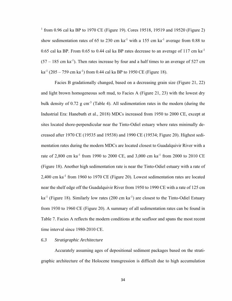
34  

1 from 0.96 cal ka BP to 1970 CE (Figure 19). Cores 19518, 19519 and 19520 (Figure 2)

show sedimentation rates of 65 to 230 cm ka-1 with a 155 cm ka-1 average from 0.88 to

0.65 cal ka BP. From 0.65 to 0.44 cal ka BP rates decrease to an average of 117 cm ka-1

(57 – 185 cm ka-1). Then rates increase by four and a half times to an average of 527 cm

ka-1 (205 – 759 cm ka-1) from 0.44 cal ka BP to 1950 CE (Figure 18).

Facies B gradationally changed, based on a decreasing grain size (Figure 21, 22)

and light brown homogeneous soft mud, to Facies A (Figure 21, 23) with the lowest dry

bulk density of 0.72 g cm-3 (Table 4). All sedimentation rates in the modern (during the

Industrial Era: Hanebuth et al., 2018) MDCs increased from 1950 to 2000 CE, except at

sites located shore-perpendicular near the Tinto-Odiel estuary where rates minimally de-

creased after 1970 CE (19535 and 19538) and 1990 CE (19534; Figure 20). Highest sedi-

mentation rates during the modern MDCs are located closest to Guadalquivir River with a

rate of 2,800 cm ka-1 from 1990 to 2000 CE, and 3,000 cm ka-1 from 2000 to 2010 CE

(Figure 18). Another high sedimentation rate is near the Tinto-Odiel estuary with a rate of

2,400 cm ka-1 from 1960 to 1970 CE (Figure 20). Lowest sedimentation rates are located

near the shelf edge off the Guadalquivir River from 1950 to 1990 CE with a rate of 125 cm

ka-1 (Figure 18). Similarly low rates (200 cm ka-1) are closest to the Tinto-Odiel Estuary

from 1930 to 1960 CE (Figure 20). A summary of all sedimentation rates can be found in

Table 7. Facies A reflects the modern conditions at the seafloor and spans the most recent

time interval since 1980-2010 CE.

6.3 Stratigraphic Architecture

Accurately assuming ages of depositional sediment packages based on the strati-

graphic architecture of the Holocene transgression is difficult due to high accumulation

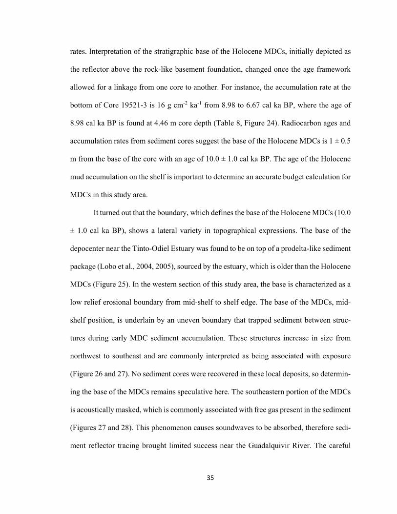
35  

rates. Interpretation of the stratigraphic base of the Holocene MDCs, initially depicted as

the reflector above the rock-like basement foundation, changed once the age framework

allowed for a linkage from one core to another. For instance, the accumulation rate at the

bottom of Core 19521-3 is 16 g cm-2 ka-1 from 8.98 to 6.67 cal ka BP, where the age of

8.98 cal ka BP is found at 4.46 m core depth (Table 8, Figure 24). Radiocarbon ages and

accumulation rates from sediment cores suggest the base of the Holocene MDCs is 1 ± 0.5

m from the base of the core with an age of 10.0 ± 1.0 cal ka BP. The age of the Holocene

mud accumulation on the shelf is important to determine an accurate budget calculation for

MDCs in this study area.

It turned out that the boundary, which defines the base of the Holocene MDCs (10.0

± 1.0 cal ka BP), shows a lateral variety in topographical expressions. The base of the

depocenter near the Tinto-Odiel Estuary was found to be on top of a prodelta-like sediment

package (Lobo et al., 2004, 2005), sourced by the estuary, which is older than the Holocene

MDCs (Figure 25). In the western section of this study area, the base is characterized as a

low relief erosional boundary from mid-shelf to shelf edge. The base of the MDCs, mid-

shelf position, is underlain by an uneven boundary that trapped sediment between struc-

tures during early MDC sediment accumulation. These structures increase in size from

northwest to southeast and are commonly interpreted as being associated with exposure

(Figure 26 and 27). No sediment cores were recovered in these local deposits, so determin-

ing the base of the MDCs remains speculative here. The southeastern portion of the MDCs

is acoustically masked, which is commonly associated with free gas present in the sediment

(Figures 27 and 28). This phenomenon causes soundwaves to be absorbed, therefore sedi-

ment reflector tracing brought limited success near the Guadalquivir River. The careful

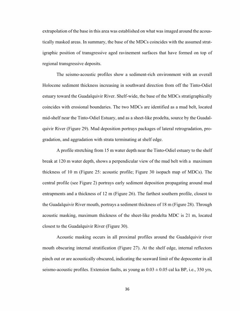
36  

extrapolation of the base in this area was established on what was imaged around the acous-

tically masked areas. In summary, the base of the MDCs coincides with the assumed strat-

igraphic position of transgressive aged ravinement surfaces that have formed on top of

regional transgressive deposits.

The seismo-acoustic profiles show a sediment-rich environment with an overall

Holocene sediment thickness increasing in southward direction from off the Tinto-Odiel

estuary toward the Guadalquivir River. Shelf-wide, the base of the MDCs stratigraphically

coincides with erosional boundaries. The two MDCs are identified as a mud belt, located

mid-shelf near the Tinto-Odiel Estuary, and as a sheet-like prodelta, source by the Guadal-

quivir River (Figure 29). Mud deposition portrays packages of lateral retrogradation, pro-

gradation, and aggradation with strata terminating at shelf edge.

A profile stretching from 15 m water depth near the Tinto-Odiel estuary to the shelf

break at 120 m water depth, shows a perpendicular view of the mud belt with a maximum

thickness of 10 m (Figure 25: acoustic profile; Figure 30 isopach map of MDCs). The

central profile (see Figure 2) portrays early sediment deposition propagating around mud

entrapments and a thickness of 12 m (Figure 26). The farthest southern profile, closest to

the Guadalquivir River mouth, portrays a sediment thickness of 18 m (Figure 28). Through

acoustic masking, maximum thickness of the sheet-like prodelta MDC is 21 m, located

closest to the Guadalquivir River (Figure 30).

Acoustic masking occurs in all proximal profiles around the Guadalquivir river

mouth obscuring internal stratification (Figure 27). At the shelf edge, internal reflectors

pinch out or are acoustically obscured, indicating the seaward limit of the depocenter in all

seismo-acoustic profiles. Extension faults, as young as 0.03 ± 0.05 cal ka BP, i.e., 350 yrs,

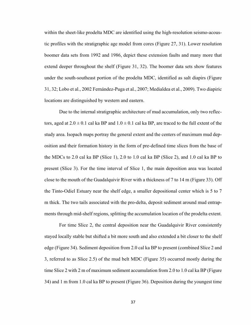
37  

within the sheet-like prodelta MDC are identified using the high-resolution seismo-acous-

tic profiles with the stratigraphic age model from cores (Figure 27, 31). Lower resolution

boomer data sets from 1992 and 1986, depict these extension faults and many more that

extend deeper throughout the shelf (Figure 31, 32). The boomer data sets show features

under the south-southeast portion of the prodelta MDC, identified as salt diapirs (Figure

31, 32; Lobo et al., 2002 Fernández-Puga et al., 2007; Medialdea et al., 2009). Two diapiric

locations are distinguished by western and eastern.

Due to the internal stratigraphic architecture of mud accumulation, only two reflec-

tors, aged at 2.0 ± 0.1 cal ka BP and 1.0 ± 0.1 cal ka BP, are traced to the full extent of the

study area. Isopach maps portray the general extent and the centers of maximum mud dep-

osition and their formation history in the form of pre-defined time slices from the base of

the MDCs to 2.0 cal ka BP (Slice 1), 2.0 to 1.0 cal ka BP (Slice 2), and 1.0 cal ka BP to

present (Slice 3). For the time interval of Slice 1, the main deposition area was located

close to the mouth of the Guadalquivir River with a thickness of 7 to 14 m (Figure 33). Off

the Tinto-Odiel Estuary near the shelf edge, a smaller depositional center which is 5 to 7

m thick. The two tails associated with the pro-delta, deposit sediment around mud entrap-

ments through mid-shelf regions, splitting the accumulation location of the prodelta extent.

For time Slice 2, the central deposition near the Guadalquivir River consistently

stayed locally stable but shifted a bit more south and also extended a bit closer to the shelf

edge (Figure 34). Sediment deposition from 2.0 cal ka BP to present (combined Slice 2 and

3, referred to as Slice 2.5) of the mud belt MDC (Figure 35) occurred mostly during the

time Slice 2 with 2 m of maximum sediment accumulation from 2.0 to 1.0 cal ka BP (Figure

34) and 1 m from 1.0 cal ka BP to present (Figure 36). Deposition during the youngest time

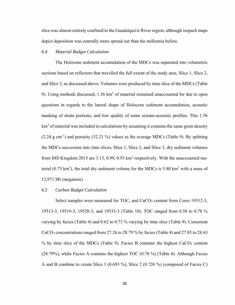
38  

slice was almost entirely confined to the Guadalquivir River region, although isopach maps

depict deposition was centrally more spread out than the millennia before.

6.4 Material Budget Calculation

The Holocene sediment accumulation of the MDCs was separated into volumetric

sections based on reflectors that travelled the full extent of the study area, Slice 1, Slice 2,

and Slice 3, as discussed above. Volumes were produced by time slice of the MDCs (Table

9). Using methods discussed, 1.56 km3 of material remained unaccounted for due to open

questions in regards to the lateral shape of Holocene sediment accumulation, acoustic

masking of strata portions, and low quality of some seismo-acoustic profiles. This 1.56

km3 of material was included in calculations by assuming it contains the same grain density

(2.24 g cm-1) and porosity (52.21 %) values as the average MDCs (Table 9). By splitting

the MDCs succession into time slices, Slice 1, Slice 2, and Slice 3, dry sediment volumes

from IHS Kingdom 2015 are 3.13, 0.99, 0.93 km3 respectively. With the unaccounted ma-

terial (0.75 km3), the total dry sediment volume for the MDCs is 5.80 km3 with a mass of

12,971 Mt (megatons).

6.5 Carbon Budget Calculation

Select samples were measured for TOC, and CaCO3 content from Cores 19512-3,

19513-3, 19519-3, 19520-3, and 19535-3 (Table 10). TOC ranged from 0.58 to 0.78 %

varying by facies (Table 4) and 0.62 to 0.73 % varying by time slice (Table 9). Consistent

CaCO3 concentrations ranged from 27.26 to 28.79 % by facies (Table 4) and 27.85 to 28.63

% by time slice of the MDCs (Table 9). Facies B contains the highest CaCO3 content

(28.79%), while Facies A contains the highest TOC (0.78 %) (Table 4). Although Facies

A and B combine to create Slice 3 (0.693 %), Slice 2 (0.726 %) (composed of Facies C)

39  

contains a higher total organic content (Table 9). These values, when combined with the

volumetric and mass calculations lead to a qualitative approximation of the retention of

marine and terrigenous carbon by the MDCs. For CaCO3 a total volume of 1.63 km3 and a

mass of 3637 Mt is calculated (Table 9). TOC has a total mass of 85 Mt (Table 9).

40  

7.0 Interpretation and Discussion

7.1 Mud Depocenter Evolution: Influences on Accumulation and Stratigraphy

Areas of low sediment accumulation in the early Holocene (> 6.5 cal ka BP) were

composed of dark greenish silts with abundant shell fragments, while material younger

than 6.5 cal ka BP contained lighter grayish homogenous muds (Figures 21, 23). Muds

from a terrigenous material are commonly associated with Fe-enriched material (Hanebuth

et al., 2015b) and the color change may potentially point to a change in sediment source:

This trend towards a stronger terrigenous contribution is also clearly reflected by a gradual

upward shift towards lower ln Ca/Fe values (Figures 13, 15, 21).

7.1.1 Holocene Transgression to 6.5 cal ka BP

After the last transgression began about 19 cal ka BP (Hernández-Molina et al.,

1994; Hanebuth et al., 2009), the base of the MDCs is defined as approximately 10.0 ± 1.0

cal ka BP. The lowermost Facies F and E are composed of muddy silt with chaotic sorting

and abundant shell fragments (Figure 21, 23). Most of the carbonate material is deterio-

rated, stained and fragmented, which points to reworking processes during transgression.

The slightly lower Ca/Fe ratio (Figures 13, 15), compared to younger facies, is possibly

affected by the larger grain size (Figure 21, 22) of material indicating a less representative

increase in Fe. The two Facies show a retrogradational deposition pattern caused by back-

stepping sedimentation as a results of a material influx which was unable to keep up with

a rapidly rising sea level. All strata terminate at the shelf break, making it challenging to

distinguish between retrogradational, aggradational, and low angle progradational

41  

sequences. In combination with absolute dating, the base of the Holocene MDCs is com-

posed of sediment deposited during a transgressive systems tract (TST) (Figures 21, 23),

which is normally not well preserved (Lobo et al., 2001, 2004). Mendes et al. (2012) found

sedimentation rates in the mud body offshore of the Guadiana River (around 10 cm ka-1),

compared to the variable 17 to 35 cm ka-1 in the mud belt MDC off shore of the Tinto-

Odiel Estuary (Figure 29; Table 7). Rates of accumulation (taking into consideration dry

bulk density) during this stage were as low as 16 to 46 g cm-2 ka-1 (Figure 24, Table 8).

An erosive boundary was located between and around topographic structures that

locally confined the northwestern base of the prodelta MDC (Figure 29), which can be

easily seen on the shore-facing side of these elevations (Figures 26, 37). Boomer data sets

show that these structures are characterized by chaotic internal reflection at depths 55 to

65 m below modern sea level. This depth suggests that these entrapping structures were

once a chain of exposed islands, possibly ca. 8.2 cal ka BP (MWP-2) (Lobo et al., 2001).

Distinguishing whether sediment naturally deposited on the landward side of these struc-

tures as a kind of lagoonal facies, or whether these depositional packages still experienced

deformation due to local uplift of the rocky obstacles, cannot be resolved by the existing

data set. Overall, internal clinoform formation inside, illustrates a backstepping pattern

consistent with the retrogradation dynamics of a TST. Once the accommodation space be-

tween these structures filled, possibly at different times during transgression, the weight of

the overbearing sediment may have started to cause subsidence of the structures closest to

the Guadalquivir River (Figure 37). Acoustic masking, due to gas presence, near the Gua-

42  

dalquivir River hides most material from the TST (Figures 27, 28, 32, 37). Faulting be-

tween structures matched with draping offsets of major reflectors indicates the base of the

prodelta MDC has undergone rates of subsidence after material deposited (Figure 37).

7.1.2 Maximum Flooding Surface

A maximum flooding surface (mfs), occurred ca. 6.5 cal ka BP (Dabrio et al., 2000;

Lario et al., 2002), i.e., at the boundary between Facies E and D (Figure 21, 23), when sea

level reached its most landward point in flooding the continent (Van Wagoner et al., 1988).

At times, the boundary-like reflector depicting the mfs is sharp, indicating non-deposition,

condensation of time, or even erosion (Figure 21). The sediment deposited just below and

above this boundary is characterized by elevated values in the ln Ca/Fe ratio (Figures 13,

15, 21) indicating that the material was dominantly supplied from marine sources (Hane-

buth et al., 2015b). This finding underlines the interruption in terrigenous supply during

maximum transgression at about 6.5 cal ka BP. At this point, the high sea level has stabi-

lized, creating the widest accommodation space on the continental shelf and inside the es-

tuaries.

7.1.3 Highstand Depositional System

Following the mfs, sea level began to stabilize towards its present day position al-

lowing for a HST to develop with deposits characterized by laterally, expanding aggrada-

tional sheets and low-angle progradational clinoforms (Figure 6; Van Wagoner et al., 1988;

Lobo et al., 2005). Grain size decrease and a constant increase in terrigenous material con-

tinues at a constant rate to present day formation of the MDCs (Figures 13, 15, 22).

While the rate of sea level rise slowed from 6.5 to 3.2 BP (Figure 7), strong long-

shore currents displaced large amounts of sediment along the coast and created a sand spit

43  

around the mouth of the Tinto-Odiel Estuary, leading to partial enclosure of the estuary

(Lario et al., 2002). During this stage, infilling of the estuary was characterized by massive

mud deposition (López-González et al., 2006). The low accumulation rates (3 to 7 g cm-2

ka-1) between 6.67 and 5.79 cal ka BP found off the Tinto-Odiel Estuary can be caused by

the high quantity of riverine mud being captured in the newly formed estuary (Table 8;

Figure 23).

Mendes et al. (2012) found sedimentation rates to be lower in the prodeltaic wedge

off shore of the Guadiana River (52 cm ka-1 from 3.75 to 1.3 cal ka BP), compared to 55

to 107 cm ka-1 from 4.35 to 1.29 cal ka BP in the mud belt MDC and northwestern portion

of the prodelta MDC (Figure 29; Table 7). In summary, the accumulation rates slightly

increased shelf wide in this study area from 5 to 38 g cm-2 ka-1 from 5.79 to 2.7 cal ka BP

(Table 8; Figure 24). In the middle of this interval, Bond Event 2 occurred as early as 3.0

cal ka BP (drought-resistant vegetation: Jiménez-Moreno et al., 2015) and as late as 2.6 cal

ka BP (decline in forest cover: Jiménez-Moreno et al., 2015). Due to this temporal blurring

and the given low time resolution between 4.35 and 2.70 cal ka BP, it is hardly possible to

identify changes in accumulation rates and link them to Bond Event 2 (Table 8). Seismo-

acoustic profiles depict aggradational deposition for this time interval which might be re-

lated to the rate of sea level, thus the opening of new accommodation space, may have been

comparable to sediment available through fluvial input.

The northwestern portion of the prodelta MDC (Figure 29) is known to undergo

subsidence due to the weight of material loading (Lobo et al., 2002), continuously opening

new accommodation space. In contrast, a diapiric intrusion (Figures 27, 31, 32) close to

shelf edge, observed at the base of the prodelta MDC (Figure 29), leads to a local reduction

44  

in accommodation space. This is due to mud deposition occurring mainly from the bottom

nepheloid layer transport (gravity currents stopping to allow for accumulation: Figure 3).

Local positive obstacles can lead to a slowing of the bottom, gravity driven, current veloc-

ity thus acting as local mud traps (Hanebuth et al., 2015a). Here, deposition is not only

controlled by the accumulation space available, but possibly also by local upwelling along

the shelf edge (Current N1 in Figure 9; García-Lafuente et al., 2006), hindering sediment

deposition or increasing seafloor interaction with currents. Further discussion on the dia-

piric uplift is provided in Section 7.3 Tectonic Influence on the Geometry of the Mud Depo-

center.

A major change in the sedimentary regime occurred after 2.7 cal ka BP when accu-

mulation rates increased by three to 17 times (Figure 24). In comparison, Mendes et al.

(2012) found sedimentation rates increasing by up to only 2 times in the prodelta wedge of

the Guadiana River. Some of this increase can be attributed to region-wide mining, defor-

estation, and agriculture activities during the Roman Period, which peaked around 1.9 ±

0.2 cal ka BP (Figure 11; Martín-Puertas et al., 2010; Hanebuth et al., 2018 and references

therein). The increase in sediment accumulation can also be related to a regional climatic

change into a humid period causing higher lake levels in southern Spain that lasted from

2.6 to 1.6 cal ka BP (Martín-Puertas et al., 2008), increased sedimentation rates in rivers

(Goy et al., 1996), and overall increased aridity in the western Saharan region (Hanebuth

and Henrich, 2009). Around 1.6 cal ka BP, the depositional pattern of the prodelta MDC

(Figure 29) transitioned into a progradational system where clinoforms reached the shelf

edge and the rate of accumulation assumedly surpassed the rates in sea level rise and sub-

sidence. The colder and dryer influence related to Bond Event 1 (1.4 cal ka BP), which

45  

occurred during or right after the termination of the Roman Empire, might be reflected by

a slight noticeable decrease in accumulation rate from 1.95 to 1.42 cal ka BP (Figure 24).

Slightly elevated accumulation rates around 1.0 cal ka BP, compared to the 600 yrs

before, is linked to the extremely high precipitation that occurred throughout the Iberian

Peninsula around 0.95 ka BP (Abrantes et al., 2017). In contrast, a locally restricted aridi-

fication event around 1.0 cal ka BP was confirmed in cores from Doñana National Park,

Spain (Jiménez-Moreno et al., 2015). This conflicting finding may indicate locally re-

stricted precipitation events affecting fluvial sediment influx to the MDCs.

The decreasing and increasing accumulation rate, depending on MDC location,

from 0.7 to 0.4 cal ka BP (Table 8; Figure 24) can be attributed to intense, but less frequent

precipitation events during the warm and generally dry MCA (1.05 to 0.7 cal ka BP) ex-

tending into the LIA (0.65 to 0.15 cal ka BP) (Nieto-Moreno et al., 2011; Wanner et al.,

2015; Abrantes et al., 2017). The prodelta MDC (Figure 29) formed larger progradational

clinoforms caused by increased flood frequency until about 0.2 cal ka BP (enhanced fresh-

water input Western Mediterranean Sea: Nieto-Moreno et al., 2011; 0.82 to 0.09 cal ka BP

Old Yellow River delta, South China Sea: Liu et al., 2013; 0.28 to 0.25 cal ka BP Rhone

River delta, Western Mediterranean Sea: Fanget et al., 2014). Due to core location, accu-

mulation rates collected during the formation of these larger progradational clinoforms is

not accurately represented with this data set (Table 8; Figure 24)

Lower accumulation rates between 0.7 to 0.4 cal ka BP (Table 8; Figure 24) of the

mud belt MDC (Figure 29) persisted during the LIA due to a dry regional climate regime

and infrequent precipitation events (0.65 to 0.15 cal ka BP; Nieto-Moreno et al., 2011;

46  

Abrantes et al., 2017). The ln (Ca/Fe) ratios depict an increase in terrestrial influence (Fig-

ures 13, 15, 21). The enhanced terrestrial signal may have been a regional difference be-

tween the Tinto-Odiel Estuary, Guadalquivir River, or Guadiana River locations or other

local controlling factors affecting accumulation rates that have not been considered such

as changes in agriculture or cultivation.

Over the past 200 yrs, accumulation rates remarkably increased up to ninety times

(72 to 2,863 g cm-2 ka-1; Table 8, Figure 24) with a high degree of industrial contamination

(Figure 11; Martín-Puertas et al., 2010; Hanebuth et al., 2018). This massive increase in

material availability is probably caused by the mining and land-use activities at a regional

and industrial scale. Yet, increasing sea surface temperatures and pollen records indicate

amplified humidity and precipitation events during the past 200 yrs (Fanget et al., 2014;

Abrantes et al., 2017), potentially intensifying sediment mobility from source to sink. At

this point, the prodelta MDC (Figure 29) depicts a switch towards an aggradational clino-

form pattern. The general increase in accumulation rates, during the Industrial Era, might

reflect an expansion of the regional land-use, often accompanied with deforestation and

soil erosion (Table 8; Figure 24). Although the Guadalquivir River hosts 15 major dams

built since the 1960’s (Hanebuth et al., 2018), which significantly interrupt the sediment

influx to the shelf, the accumulation rate (Figure 24) at the prodelta MDC (Figure 29) per-

sistently increased. This trend may be owed to the frequent occurrence of flood layers from

storms events that eroded additional material from the lower Guadalquivir region (Abrantes

et al., 2017; Hanebuth et al., 2018). Cores within the mud belt MDC (Figure 29), however,

contained decreased accumulation rates by about 40% over the past 40 yrs (1970 to 1990

47  

CE ) (Sites 19535 and 19538; Table 8). Close to the Tinto-Odiel Estuary, Site 19534, con-

tains a decrease of 60% from 1990 to 2000 CE (Table 8). This local reduction in sediment

availability cannot be explained by the existing data sets. It might be related to increased

bottom trawling (Oberle et al., 2014) leading to massive sediment resuspension; or an ef-

ficient damming in the small catchment area of the Tinto and Odiel Rivers, or further and

larger Guadiana River, trapping sediment inside rivers.

As a summary, the accumulation rates of the MDC increase substantially at about

2.7 ± 0.2 ka BP (Table 8; Figure 24). In contrast, the Holocene accumulation rates recon-

structed from southwestern Spanish estuaries (Lario et al., 2002) showed that early sedi-

ment accumulation occurred at a high rate of 5 mm yr-1 between 10 to 6.5 cal ka BP, while

it substantially lowers to 1.5 mm yr-1 afterwards (6.5 cal ka BP to present). This transition

occurred around 6.5 cal ka BP when the accumulation rate surpassed the rate a decelerating

sea level rise (Figures 11, 24; Lario et al., 2002; Lantzsch et al., 20009, 2014). When com-

paring the general rising and accelerating trend of sedimentation rates extracted from the

MDCs with estuary rates from Lario et al. (2002), there is almost an inverse correlation

(Figure 38). During the TST, as sea level rose rapidly and shoreline retrograded, sediment

was initially being trapped inside the newly formed estuaries.

Lario et al. (2002) indicated a definite change in sediment accumulation between 7

and 6 cal ka BP, whereas accumulation rates in the MDC did not depict a major increase

until 3 to 2 cal ka BP (Figure 38). This apparent delay can be due a variety of factors which

are unrelated to sea level history, such as the increase in deforestation, mining, coastal land-

use (Hanebuth et al., 2018 and references therein), but also a humid climatic event (Martín-

Puertas et al., 2008; Goy et al., 1996); all increasing the sediment flux to the shelf. Another

48  

reason, although speculative, could be that the current oceanographic circulation patterns

may not have been well established before 2.7 cal ka BP, limiting regional-scale sediment

movement. Even after taking these scenarios into consideration, the time delay could be

due to a gap in data coverage between the modern coastline and the 20 m mark in water

depth. The inner shelf zone may have accumulated material before the mid-shelf region

received sediment, i.e., until the accommodation space on the inner shelf was filled (around

2.7 cal ka BP).

7.2 Sediment Budget Calculation

By splitting the MDC into time slices and adding them together with the unac-

counted portion of material (an extra 0.75 km3 and 1,672 Mt of sediment), the total dry

sediment sums up to a volume of 5.80 km3 and a mass of 12,980 Mt (with an error of at

least +7%, if the TWT velocity of 1,500 m/s is underestimating the real acoustic velocity

in surficial soft sediment; see Oberle et al., 2014), covering an overall area of 1,900 km2.

This time slice approach also led to the calculation of 3,637 Mt for CaCO3 and to 85 Mt

for TOC (Table 9). To place these numbers into a context, they are compared to two other

siliciclastic shelf systems which contain sediment budget calculations.

The Galicia mudbelt system off Northwest Spain contains 3.9 km3 of sediment with

a total mass of 4,035 Mt (similar uncertainty as mentioned above) over an area of 4,490

km2 (Oberle et al., 2014). Its total organic and carbonate contents sum up to 40 Mt and 174

Mt, respectively. This shelf mud depositional system started to form around 5.3 cal ka BP

(Lantzsch et al., 2009), i.e., about a millennium later than the establishment of the modern

MDC in the Gulf of Cadiz. The advantage the Oberle et al (2014) study had was that the

fluvial sediment discharge for the Galician region was roughly known. With these two

49  

parameters, the primary input, and the storage on the shelf, it was possible to calculate that

about 65 % of the fluvially supplied mud bypasses extent of the shelf eventually depositing

in the deep ocean.

The Adria mudbelt system to the east of Italy assumed that no sediment ever left

this semi-enclosed basin (Brommer et al, 2009). The study could then be used to recon-

struct the volume of later Holocene sediment discharge of various rivers draining from the

Italian Peninsula into the Adriatic Sea. The budget calculation resulted in 254,000 Mt ± 15

% for the highstand MDC over a larger area of ca. 35,000 km2. This depocenter also formed

over the past 5.5 thousand yrs when sea level stabilized.

By comparing the three systems it turns out that each individual MDC is inherently

different (Table 11). In terms of initiation age, these three systems are close to each other

and underline the important role sea level can play in open accommodation space. How-

ever, the early initiation of the transgressive Facies F and E in the Cadiz MDC corresponds

to other examples, as compiled by Hanebuth et al. (2015b and worldwide references

therein), where the shelf was inundated enough at the beginning of the Holocene to allow

for early mud accumulation. The Galician shelf is characterized by an overall exceptionally

steep shelf gradient and the Adriatic shelf shows two steps in bathymetry, therefore both

did not favor an early accumulation.

In terms of composition, the Gulf of Cadiz depocenters contain a much higher con-

tent of carbonate and organic matter than the Galician depocenter (Table 11). The average

carbonate content in the Cadiz depocenter is 28% while it is only 4% off Galicia; the aver-

age TOC in the Cadiz depocenter is 0.5%, but nearly 1% off Galicia. This difference indi-

cates that proportion of fluvial input in the mid-shelf MDC off Galicia is significantly

50  

higher compared to the Cadiz system. Thus, the role of MDCs as sinks and possible sec-

ondary sources for carbon as a component in the regional and global carbon cycle needs to

be individually considered. This makes a global calculation of med depocenter carbon re-

tention a challenge.

In terms of sediment retention, the lack in sediment supply data in the Gulf of Cadiz

does not allow for a full budget calculation or a comparison. Since the sediment export

from muddy shelf systems can vary from 0 to 90% (see Oberle et al., 2014, for worldwide

references) it is not further possible to calculate either fluvial input or export across the

shelf edge based on this new data.

7.3 Tectonic Influence on the Geometry of the Mud Depocenter

The central depositional location of the prodelta MDC (Figure 29) shows an unu-

sual stratigraphic pattern during early Holocene. Boomer data illustrates a diapiric structure

below the MDC (Figures 31, 32), which confirms the finding of salt diapirism by previous

studies (Fernández-Puga et al., 2007; Rodero et al., 1999; Lobo et al., 2002). This diapiric

(western diapir) structure caused spectacular deformation of the MDC during early Holo-

cene and led to a concentration of deposition to other areas of the shelf (Figure 32). Exten-

sion faulting is conceptually associated with diapir tectonics (Rodero et al., 1999; Lobo et

al., 2014). Initially during this study, only a few isolated faults were found and were ex-

pected to be caused by local subsidence due to compaction. After the discovery of two

diapiric intrusions, however, it became obvious that the boomer data sets show numerous

faults vertically extending far into the MDC from at least as deep as 150 m below seafloor

(Figure 31, 32).

51  

Extensional faulting is found between the western salt diapir and Guadalquivir

River, where depocenter thickness is greatest (Figures 31, 39). Salt diapirism is a wide-

spread phenomenon in the eastern part of the Gulf of Cadiz (Fernández-Puga et al., 2007;

Medialdea et al., 2009).The loading by the MDC may additionally be pushing on evaporitic

deposits located deeply below the shelf. These evaporitic deposits flow along a pressure

gradient by the overburden until it reaches a fault line where the evaporite elastically mi-

grates upward into an elevation of less pressure, creating the two identified diapir locations

(Figures 31, 32; Fernández-Puga et al., 2007). These diapiric structures are composed of

salt or a marly salt from the regional so-called Allochthonous Unit of Triassic age (Me-

dialdea et al., 2009).

As the evaporitic material moves towards the diapir, the sediment cover around the

diaper tends to subside to balance the mass lost in the subbottom, accompanied by exten-

sion fault lines (Figure 39). Surprisingly, these faults extend up into MDC strata as young

as 0.03 ± 0.05 cal ka BP, i.e., 350 yrs ago, meaning they are still active in sub-recent times

(Figure 39), with an increasing age trend towards the west. Overall, these basement struc-

tures seem to be subsiding in relation to the large sheet-like prodelta MDC (Figure 29).

The eastern diapir location contains three small diapir peaks, where the formation

capping the eastern most diapir, of the three small peaks, has penetrated into the base of

the MDC (Figure 31). Local extension faults associated with this penetration are also as

young as 0.03 ± 0.05 cal ka BP, i.e. again 350 yrs ago.

Perpendicular to the shelf edge in the southern-most seismo-acoustic profiles, an

extensional fault, which even deforms the modern seafloor was detected (Figure 39). Based

on fault orientation, the shore-side of the fault, extending inland as far as to Site 19519, has

52  

undergone subsidence related to local block tectonics (Figure 39). Due to the acoustic

masking caused by gas, it is not possible to trace the full movement of this fault (Figure

27).

Gas deposits commonly formed in relation to diapirism due to faults, often provides

both a pathway of least resistance for the gas to travel and a cap stone by upward bending

strata. Within the Gulf of Cadiz, the Allochthonous Unit and overlaying units are known

to contain a mixture of thermogenic and biogenic gas (Medialdea et al., 2009). Past the

shelf break, Boomer acoustic images depict gaseous sediment along the flank of the west-

ern diapir (Figure 40) and pockmarks caused by gas expulsion below the gaseous sediment

(Casas et al., 2003). If thermogenic gas off the Guadalquivir River travels upward through

extension faults (fault locations in relation to acoustic masking Figure 27), a capping fine-

grained sediment body would have the potential to trap and thus concentrate the gas. The

top of the gas correlates with an internal reflector, which dates at about 0.88 ± 0.05 cal ka

BP and represents the boundary between Facies C and B (Figures 21, 23).

However as a commonly found alternative to explain the shallow gas blob in front

of major river systems, the gas might simply be associated to the thick Holocene prodeltaic

sediment wedge which was sourced by the Guadalquivir River over time (Figures 27, 28).

Locations of organic rich fluvial material are favorable for microbial shallow-gas formation

as described in many other regions (Senegal shelf: Nizou et al., 2010).

7.4 Differentiation of Sediment Sources

Using the newly generated data sets, a differentiation in the influence of the various

fluvial sediment sources could not be determined and therefore remains speculative. Look-

ing at the isopach maps, Slice 3 (1.0 cal ka BP to present: Figure 36) has a larger area

53  

(1,130 km2) than Slice 2 (2.0 to 1.0 cal ka BP: Figure 34) (1,030 km2) but a smaller volume

and mass (Table 7). Maximum MDC thicknesses from Slice 3 is 5 m (Figure 36), while

Slice 2 max thickness is 7 m (Figure 34).

After 2.0 cal ka BP, sediment deposition specifically in the Tinto-Odiel portion of

the depocenter occurred mostly during Slice 2 with maximum, 2 m of sediment, (Figure

34) and 1 m, i.e., 50 % from Slice 3 (Figure 36). Deposition post-1 cal ka BP (Slice3) was

almost entirely confined to the Guadalquivir River region, although isopach maps depict

deposition was laterally more extent than the millennia before (Figure 36).

This observation can be explained by several mechanisms that influence growth

dynamics of the MDC. Current circulation patterns on the shelf may have been different

from 2.0 to 1.0 cal ka BP than modern day circulation. On the anthropogenic side, an in-

crease in river damming, (small Tinto and Odiel Rivers, or further and larger Guadiana

River) trapping sediment inside rivers (González-Ortegón et al., 2010), may have limited

sediment input. To verify this assumption, high resolution grain size measurements of cores

through central shelf, parallel to shore, should be performed. If the seemingly detached

lobe near the Tinto-Odiel Estuary is not fed by the Guadalquivir, grain size distribution

stemming from the Guadalquivir to this lobe, will depict decreasing grain size followed by

an increase. An increase in grain size can indicate a different source, as speculated, the

Guadiana River. Sediment from the Guadiana River can be transported to this location by

the NASW current (Mauritzen et al., 2001; García-Lafuente et al., 2006).

54  

8.0 Conclusions

Mud accumulation between the Tinto-Odiel Estuary and the Guadalquivir River

has previously been described as taking place in separate MDCs (Figure 4; Lobo et al.,

2004), where the outer-shelf deposits are mainly sourced by the Guadiana and mixed with

Guadalquivir-sourced material. For the mid- to inner-shelf, a prodelta wedge MDC is iden-

tified off the Guadalquivir River mouth (Figures 11, 29; Lobo et al., 2004). Due to the

lateral continuity of major internal stratigraphic reflectors across the shelf and based on the

accumulation rate reconstruction, the southeastern two thirds of this study area seem to be

sourced mainly by the Guadalquivir River. The deposit, however, also contains a mixed

heavy metal signature from the Tinto-Odiel Estuary (Hanebuth et al., 2018). The remaining

northwestern third of the study area is determined to be a portion of a mud belt MDC

sourced mainly by the Guadiana River (Figures 11, 29; Lobo et al., 2004). The closer Tinto-

Odiel Estuary may also provide material to the mud belt MDC (heavy metal signature pres-

ence: Hanebuth et al., 2018).

While the prodelta MDC (Figure 29) seems relatively unchanged over the past 2.0

cal ka BP (Figures 34, 36), the mud belt MDC (Figure 29) showed a 50% decrease in

accumulation when splitting the 2.0 cal ka BP-to-present time interval in a phase prior to

and after 1.0 cal ka BP (and particularly during the past 200 yrs). Although this assumption

remains speculative, recent damming of the Tinto and Odiel Rivers, or further and larger

Guadiana River, may have instigated a lower sediment output to the shelf causing lower

accumulation rates in the northwest sector (Figure 24, Table 8).

55  

Through accumulation rates and early Holocene ages, the base of the MDCs is es-

timated to be around 10.0 ± 1.0 cal ka BP, i.e., in earliest Holocene times. Six major suc-

cessive sedimentary facies comprise the MDC with the oldest two (F and E) depicting ret-

rogradational deposits linked to the last transgression until 6.5 cal ka BP, when sea level

stabilized close to the present day level (Figures 21, 23). The modern appearance of the

MDCs started to develop at that time, which indicates a major change in sediment availa-

bility and accumulation associated with a stable and high sea level. Accumulation rates

stayed relatively low until around 2.7 cal ka BP (Figure 24, Table 8). The following in-

crease in sediment accumulation can be linked to agricultural and mining activities during

the Roman Period on the southern Iberian Peninsula (Hanebuth et al., 2018 and references

therein) and also to a humid climatic period, which lasted from 2.6 to 1.6 cal ka BP in

southern Spain (Martín-Puertas et al., 2008; Goy et al., 1996). A drop in accumulation rates

(Figure 24, Table 8) occurred around Bond Event 1 (1.4 cal ka BP) from 1.8 to 1.4 cal ka

BP. Intense precipitation events during an arid and dry MCA (1.05 to 0.7 cal ka BP) (Nieto-

Moreno et al., 2011; Wanner et al., 2015), with extreme occurrences around 950 cal ka BP

(Abrantes et al., 2017), probably attributed to higher accumulation rates around 1.0 cal ka

BP and slightly lower, variable accumulation rates extending within the LIA (Figure 24,

Table 8). In contrast, localized decline in forest cover in Doñana National Park, Spain (Ji-

ménez-Moreno et al., 2015) indicates these intense precipitation events may differ on re-

gional scale by watershed basin. Variable accumulation rates in the mud belt MDC and

northwestern prodelta MDC (Figure 29) occur due to frequent, yet less extreme, precipita-

tion events with an arid climate persisting into the LIA (0.65 to 0.15 cal ka BP) (Abrantes

et al., 2017) until about 0.44 cal ka BP (Nieto-Moreno et al., 2011). From 0.44 to present,

56  

accumulation rates have been heavily influenced by urbanization and industrialization,

mining, river damming, possibly offshore and inshore dredging, and chronic bottom trawl-

ing (Hanebuth et al., 2018 and references therein; Figure 24, Table 8).

An increase in the terrigenous input signal (Figures 13, 15, 21: ln Ca/Fa), a fining

grain size (Figure 21, 22: ln Ti/Zr), and increasing sedimentation (Figure 18, 19, 20; Table

7) and accumulation rates (Figure 24; Table 8) all correlate to a generally more humid and

increased anthropogenic modified present day shelf.

From the base of the MDCs to 2.0 cal ka BP, 3.13 km3 weighing 6,939 Mt of sedi-

ment accumulated. After the start of the humid period, while the Roman Empire expanded

over the Iberian Peninsula, i.e., during time slice 2.0 to 1.0 cal ka BP, the depocenter accu-

mulated 0.99 km3 of sediment with a mass of 2,222 Mt. Since the MCA (1.0 cal ka BP to

present), 0.93 km3 of dry sediment accumulated with a weight of 2,138 Mt. The time slice

method used to produce the volumetric and mass budget calculations accounted for an ad-

ditional 0.27 km3 and 566 Mt of material (Table 9: synopsis of calculations).These calcu-

lations combined with the carbon contents provided a TOC mass of 85 Mt, and a CaCO3

mass of 3637 Mt with a total volume of 1.63 km3.

Surprising findings, depict extension faults persist into the modern MDC. Salt dia-

pirs, originating from the Triassic Era (Fernández-Puga et al., 2007; Medialdea et al., 2009)

are rising along older extension faults caused by compression in the NE-SW orientation

(Fernández-Puga et al., 2007; Medialdea et al., 2009). As the material is displaced, salt

diapir uplift has caused localized extension faults and controlled the location and thickness

of mud deposition on local scale (Figures 32, 33). This tectonic influence was active until

57 

0.03 ± 0.05 cal ka BP (Figures 39). As a result of this displacement, the sedimentary suc-

cession of the prodelta MDC (Figure 29) has undergone and continues to undergo subsid-

ence in correlation with other extension faults. Commonly associated with diapirs, gaseous

sediment have been found close to extension faults, evident by acoustic-masking (Figure

28) and core expansion while opening (Figure 21: Core 19517-3). However, the gaseous

sediments can be related to a high organic content present in the Guadalquivir prodelta

depocenter (Senegal shelf: Nizou et al., 2010).

There are some studies that can be conducted to bring to light some speculation

discussed or confirm proxies used. Grain size data should be collected at a future time to

corroborate the grain size proxy using ln (Ti/Zr) ratios (Figures 21, 22) and confirm or

deny source differentiation between the mud belt MDC and prodelta MDC (Figure 29). If

age resolution can be increased, climatic variability can be found on a smaller scale than

what has been presented. A closer look into the extension faults can produce rates at which

the fault has been moving, at least during the Holocene. Further study of the gas may be

able to determine if its origin is thermogenic or biogenic fueled (Medialdea et al., 2009).

If further studies of the suspended sediment and sediment bedload for all fluvial sources

are conducted, a retention budget can be complied for the shelf.

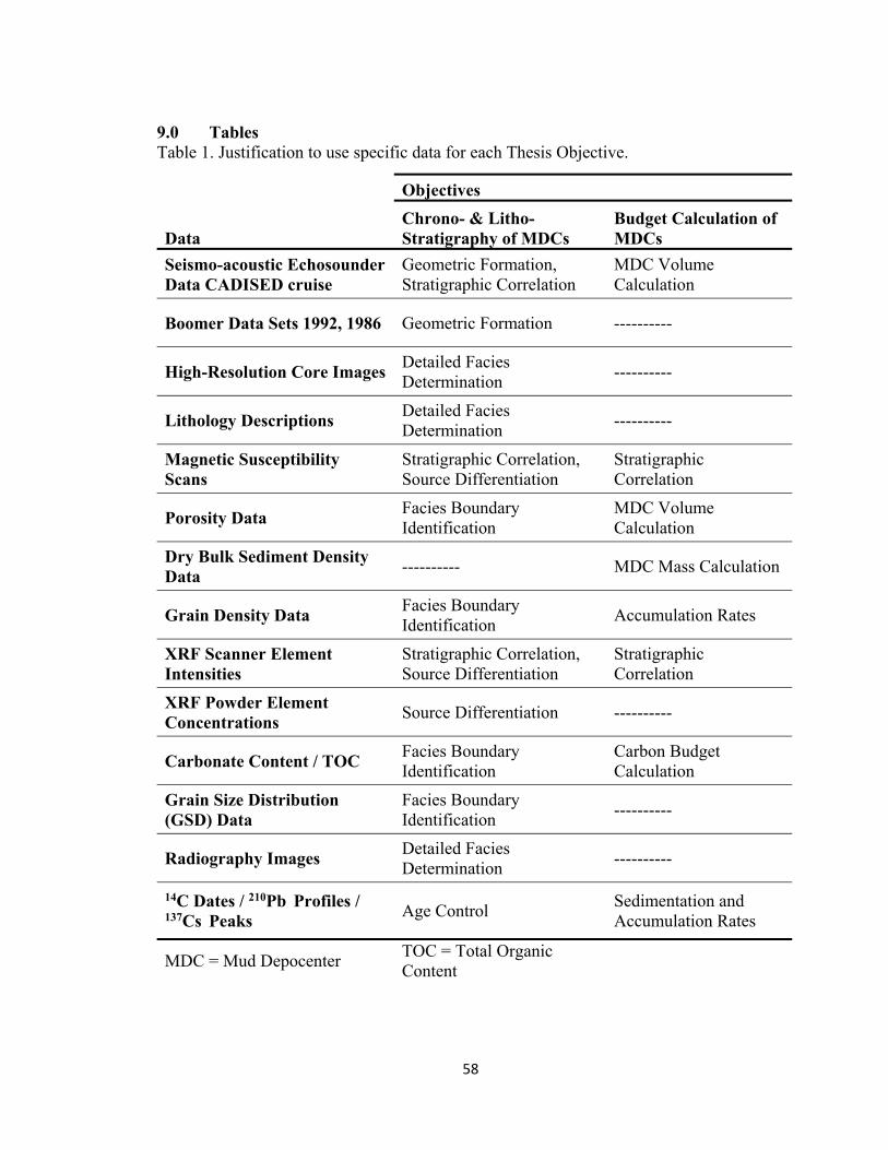
58  

9.0 Tables Table 1. Justification to use specific data for each Thesis Objective.

Objectives

Data Chrono- & Litho- Stratigraphy of MDCs

Budget Calculation of MDCs

Seismo-acoustic Echosounder Data CADISED cruise

Geometric Formation, Stratigraphic Correlation

MDC Volume Calculation

Boomer Data Sets 1992, 1986 Geometric Formation ----------

High-Resolution Core ImagesDetailed Facies Determination

----------

Lithology Descriptions Detailed Facies Determination

----------

Magnetic Susceptibility Scans

Stratigraphic Correlation, Source Differentiation

Stratigraphic Correlation

Porosity Data Facies Boundary Identification

MDC Volume Calculation

Dry Bulk Sediment Density Data

---------- MDC Mass Calculation

Grain Density Data Facies Boundary Identification

Accumulation Rates

XRF Scanner Element Intensities

Stratigraphic Correlation, Source Differentiation

Stratigraphic Correlation

XRF Powder Element Concentrations

Source Differentiation ----------

Carbonate Content / TOC Facies Boundary Identification

Carbon Budget Calculation

Grain Size Distribution (GSD) Data

Facies Boundary Identification

----------

Radiography Images Detailed Facies Determination

----------

14C Dates / 210Pb Profiles / 137Cs Peaks

Age Control Sedimentation and Accumulation Rates

MDC = Mud Depocenter TOC = Total Organic Content

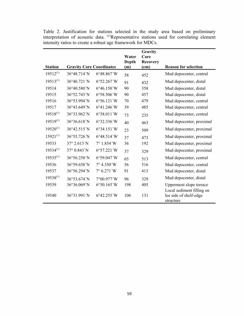
59  

Table 2. Justification for stations selected in the study area based on preliminary interpretation of acoustic data. (1)Representative stations used for correlating element intensity ratios to create a robust age framework for MDCs.

Station Gravity Core Coordinates

Water Depth (m)

Gravity Core Recovery (cm) Reason for selection

19512(1) 36°48.714´N 6°48.867´W 58 452 Mud depocenter, central

19513(1) 36°46.721´N 6°52.267´W 91 432 Mud depocenter, distal

19514 36°40.580´N 6°46.150´W 90 358 Mud depocenter, distal

19515 36°52.743´N 6°58.506´W 90 457 Mud depocenter, distal

19516 36°53.994´N 6°56.121´W 70 479 Mud depocenter, central

19517 36°43.649´N 6°41.246´W 39 485 Mud depocenter, central

19518(1) 36°33.962´N 6°38.011´W 73 235 Mud depocenter, central

19519(1) 36°36.618´N 6°32.336´W 40 463 Mud depocenter, proximal

19520(1) 36°42.515´N 6°34.151´W 23 509 Mud depocenter, proximal

15921(1) 36°55.726´N 6°48.514´W 37 473 Mud depocenter, proximal

19533 37° 2.613´N 7° 1.854´W 36 192 Mud depocenter, proximal

19534(1) 37° 0.843´N 6°57.221´W 37 329 Mud depocenter, proximal

19535(1) 36°56.258´N 6°59.047´W 65 513 Mud depocenter, central

19536 36°59.658´N 7° 4.350´W 56 516 Mud depocenter, central

19537 36°56.294´N 7° 6.271´W 91 413 Mud depocenter, distal

19538(1) 36°53.674´N 7°00.977´W 96 329 Mud depocenter, distal

19539 36°36.069´N 6°50.165´W 198 405 Uppermost slope terrace

19540 36°31.991´N 6°42.255´W 106 131 Local sediment filling on lee side of shelf-edge structure

 

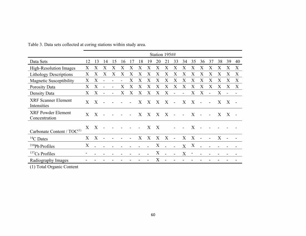
60  

Table 3. Data sets collected at coring stations within study area.

Station 195##

Data Sets 12 13 14 15 16 17 18 19 20 21 33 34 35 36 37 38 39 40

High-Resolution Images X X X X X X X X X X X X X X X X X X

Lithology Descriptions X X X X X X X X X X X X X X X X X X

Magnetic Susceptibility X X - - - X X X X X X X X X X X X X

Porosity Data X X - - X X X X X X X X X X X X X X

Density Data X X - - X X X X X X - - X X - X - -

XRF Scanner Element Intensities

X X - - - - X X X X - X X - - X X -

XRF Powder Element Concentration

X X - - - - X X X X - - X - - X X -

Carbonate Content / TOC(1) X X - - - - - X X - - X - - - - -

14C Dates X X - - - - X X X X - X X - - X - -

210Pb Profiles X - - - - - - - X - - X X - - - - - 137Cs Profiles - - - - - - - - X - - X - - - - - -

Radiography Images - - - - - - - - X - - - - - - - - -

(1) Total Organic Content

 

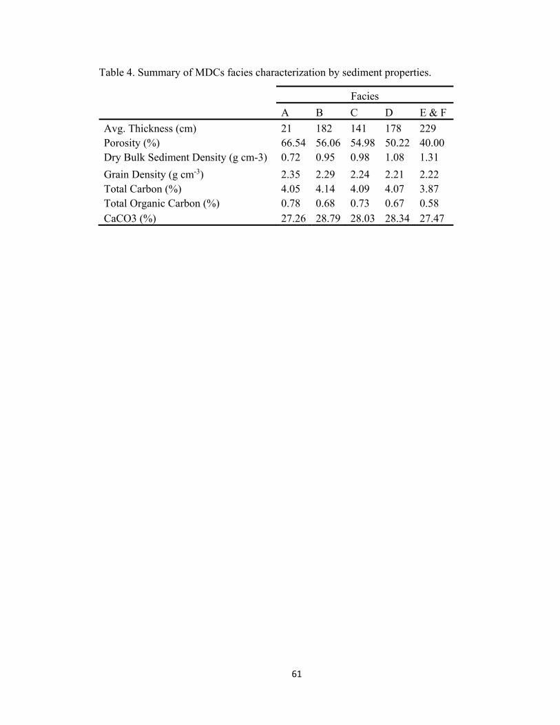
61  

Table 4. Summary of MDCs facies characterization by sediment properties.

Facies

A B C D E & F

Avg. Thickness (cm) 21 182 141 178 229 Porosity (%) 66.54 56.06 54.98 50.22 40.00 Dry Bulk Sediment Density (g cm-3) 0.72 0.95 0.98 1.08 1.31

Grain Density (g cm-3) 2.35 2.29 2.24 2.21 2.22 Total Carbon (%) 4.05 4.14 4.09 4.07 3.87 Total Organic Carbon (%) 0.78 0.68 0.73 0.67 0.58 CaCO3 (%) 27.26 28.79 28.03 28.34 27.47

 

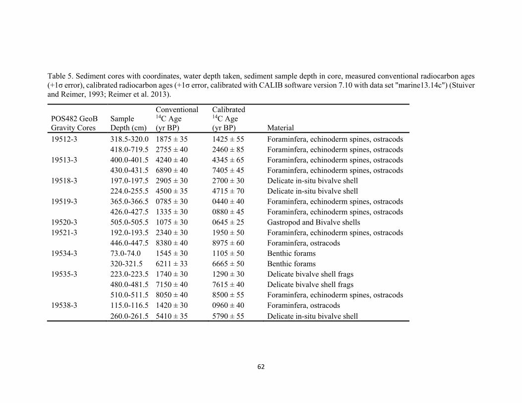
62  

Table 5. Sediment cores with coordinates, water depth taken, sediment sample depth in core, measured conventional radiocarbon ages (+1σ error), calibrated radiocarbon ages (+1σ error, calibrated with CALIB software version 7.10 with data set "marine13.14c") (Stuiver and Reimer, 1993; Reimer et al. 2013).

POS482 GeoB Gravity Cores

Sample Depth (cm)

Conventional 14C Age (yr BP)

Calibrated 14C Age (yr BP) Material

19512-3 318.5-320.0 1875 ± 35 1425 ± 55 Foraminfera, echinoderm spines, ostracods

418.0-719.5 2755 ± 40 2460 ± 85 Foraminfera, echinoderm spines, ostracods 19513-3 400.0-401.5 4240 ± 40 4345 ± 65 Foraminfera, echinoderm spines, ostracods

430.0-431.5 6890 ± 40 7405 ± 45 Foraminfera, echinoderm spines, ostracods 19518-3 197.0-197.5 2905 ± 30 2700 ± 30 Delicate in-situ bivalve shell

224.0-255.5 4500 ± 35 4715 ± 70 Delicate in-situ bivalve shell 19519-3 365.0-366.5 0785 ± 30 0440 ± 40 Foraminfera, echinoderm spines, ostracods

426.0-427.5 1335 ± 30 0880 ± 45 Foraminfera, echinoderm spines, ostracods 19520-3 505.0-505.5 1075 ± 30 0645 ± 25 Gastropod and Bivalve shells 19521-3 192.0-193.5 2340 ± 30 1950 ± 50 Foraminfera, echinoderm spines, ostracods

446.0-447.5 8380 ± 40 8975 ± 60 Foraminfera, ostracods 19534-3 73.0-74.0 1545 ± 30 1105 ± 50 Benthic forams

320-321.5 6211 ± 33 6665 ± 50 Benthic forams 19535-3 223.0-223.5 1740 ± 30 1290 ± 30 Delicate bivalve shell frags

480.0-481.5 7150 ± 40 7615 ± 40 Delicate bivalve shell frags

510.0-511.5 8050 ± 40 8500 ± 55 Foraminfera, echinoderm spines, ostracods 19538-3 115.0-116.5 1420 ± 30 0960 ± 40 Foraminfera, ostracods 260.0-261.5 5410 ± 35 5790 ± 55 Delicate in-situ bivalve shell

 

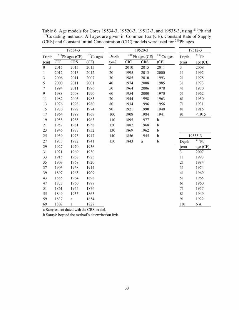
63  

Table 6. Age models for Cores 19534-3, 19520-3, 19512-3, and 19535-3, using 210Pb and 137Cs dating methods. All ages are given in Common Era (CE). Constant Rate of Supply (CRS) and Constant Initial Concentration (CIC) models were used for 210Pb ages.

CIC CRS CIC CRS0 2015 2015 2015 5 2010 2015 2011 3 20081 2012 2013 2012 20 1995 2013 2000 11 19923 2006 2011 2007 30 1985 2010 1993 21 19785 2000 2011 2001 40 1974 2008 1985 31 19737 1994 2011 1996 50 1964 2006 1978 41 19709 1988 2008 1990 60 1954 2000 1970 51 196211 1982 2003 1985 70 1944 1998 1963 61 195013 1976 1998 1980 80 1934 1996 1956 71 193115 1970 1992 1974 90 1921 1990 1948 81 191617 1964 1988 1969 100 1908 1984 1941 91 <191519 1958 1985 1963 110 1895 1977 b21 1952 1981 1958 120 1882 1968 b23 1946 1977 1952 130 1869 1962 b25 1939 1975 1947 140 1856 1945 b27 1933 1972 1941 150 1843 a b29 1927 1970 193631 1921 1969 1930 3 200733 1915 1968 1925 11 199335 1909 1968 1920 21 198437 1903 1968 1914 31 197439 1897 1965 1909 41 196943 1885 1964 1898 51 196547 1873 1960 1887 61 196051 1861 1945 1876 71 195755 1849 1935 1865 81 194959 1837 a 1854 91 192269 1807 a 1827 101 NAa Samples not dated with the CRS model.b Sample beyond the method’s determination limit.

Depth (cm)

19534-3

Depth (cm)

210Pb ages (CE) 137Cs ages (CE)

19520-3210Pb ages (CE) 137Cs ages

(CE)

19512-3

Depth (cm)

210Pb age (CE)

Depth (cm)

210Pb age (CE)

19535-3

 

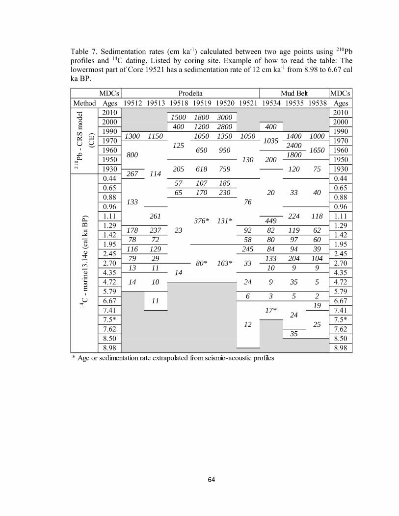
64  

Table 7. Sedimentation rates (cm ka-1) calculated between two age points using 210Pb profiles and 14C dating. Listed by coring site. Example of how to read the table: The lowermost part of Core 19521 has a sedimentation rate of 12 cm ka-1 from 8.98 to 6.67 cal ka BP.

MDCs MDCsMethod Ages 19512 19513 19518 19519 19520 19521 19534 19535 19538 Ages

* Age or sedimentation rate extrapolated from seismio-acoustic profiles

Prodelta Mud Belt

20101500 1800 3000

20001200 2800

20102000

400 400

1950 1950

0.44 0.4457 107

800

19702400

1960 1960

10501035

10001990 1990

205 6181930

1650200

185267

20 40

1.4272 58 80

1.29237 92 82 119 62

1930

65 170 230

133 204

24 9

78178

449

114

650 950130

224

2.702.451.95

760.96

0.650.88

245

1.11

0.65

118

7.5*

210 P

b -

CR

S m

odel

(CE

) 1300 1150125

1050 1350 1400

1800

759

1970

120

14C

- m

arin

e13.

14c

(cal

ka

BP

)

35

133

116

33

261

97 60

104

1.29

7.41

5.796.67

4.35

79 29

1.42

376* 131*

0.961.11

94

8.50

2.70

5

2.45

8.50

4.3513 11

1410

80*9 9

14 104.72

1.95

33

23

4.72

7.417.5*7.62

5.796.67

5

12

17*24

2

8.98 8.98

19

2535

116 3

75

163*

7.62

39

0.88

129 84

 

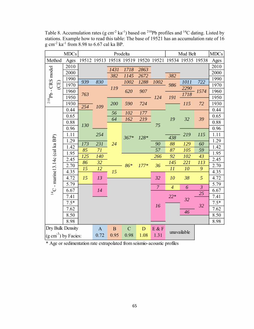
65  

Table 8. Accumulation rates (g cm-2 ka-1) based on 210Pb profiles and 14C dating. Listed by stations. Example how to read this table: The base of 19521 has an accumulation rate of 16 g cm-2 ka-1 from 8.98 to 6.67 cal ka BP.

MDCs MDCsMethod Ages 19512 19513 19518 19519 19520 19521 19534 19535 19538 Ages

* Age or sedimentation rate extrapolated from seismio-acoustic profiles

Prodelta Mud Belt

1960

0.65

1.42

210 P

b -

CR

S m

odel

(CE

)

2010 20101431 1718 2863

2000

7221970 1970

763

109

620 907124

22901574

1990

0.96

1990939 830

1191002 1288 1002

9861011

2000382 1145 2672 382

1960191

17181950 1950

2001930 1930254

19

219 1151.11 1.11438

1.29 1.29173

1.42

39

231 90 88 129 6059

254

85 71 57 87 105

590 724 115 72

177*

266 92 102 43145 221 113

14C

- m

arin

e13.

14c

(cal

ka

BP

)

0.44 0.44

130

560.65

64 162 2190.88 0.88

24367* 128*

0.96

102 177

7532

2.45 2.4586 32

362.70 2.704.35 4.35

15 13 4.72

15 1215

11 10 9

38 54.72

125 140

86*

1.95 1.95

16

22*32

257.41 7.41

5.79 5.7914

7 4 6

32 10

Dry Bulk Density

(g cm-3) by Facies:

8.98 8.98

unavailableE & F1.31

D1.08

C0.98

B0.95

A 0.72

327.5* 7.5*7.62 7.62

468.50 8.50

36.67 6.67

 

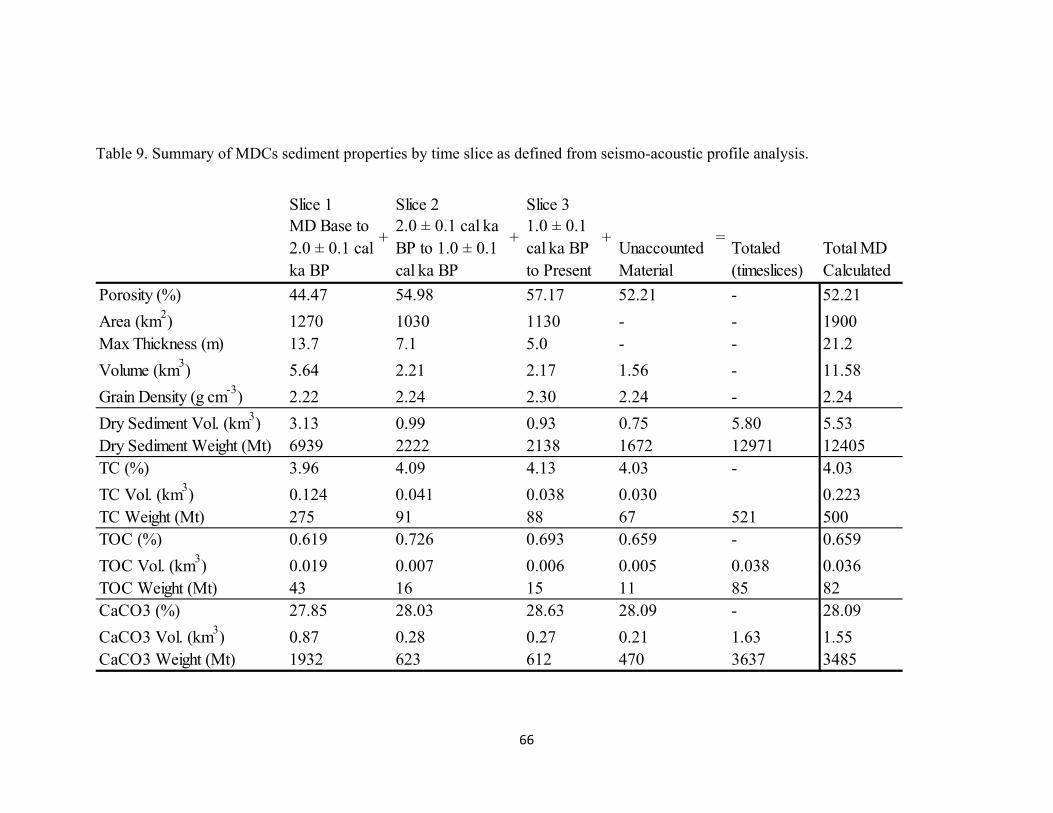
66  

Table 9. Summary of MDCs sediment properties by time slice as defined from seismo-acoustic profile analysis.

Slice 1 Slice 2 Slice 3MD Base to 2.0 ± 0.1 cal ka BP

2.0 ± 0.1 cal ka BP to 1.0 ± 0.1 cal ka BP

1.0 ± 0.1 cal ka BP to Present

Unaccounted Material

Totaled (timeslices)

Total MD Calculated

Porosity (%) 44.47 54.98 57.17 52.21 - 52.21

Area (km2) 1270 1030 1130 - - 1900Max Thickness (m) 13.7 7.1 5.0 - - 21.2

Volume (km3) 5.64 2.21 2.17 1.56 - 11.58

Grain Density (g cm-3) 2.22 2.24 2.30 2.24 - 2.24

Dry Sediment Vol. (km3) 3.13 0.99 0.93 0.75 5.80 5.53Dry Sediment Weight (Mt) 6939 2222 2138 1672 12971 12405TC (%) 3.96 4.09 4.13 4.03 - 4.03

TC Vol. (km3) 0.124 0.041 0.038 0.030 0.223TC Weight (Mt) 275 91 88 67 521 500TOC (%) 0.619 0.726 0.693 0.659 - 0.659

TOC Vol. (km3) 0.019 0.007 0.006 0.005 0.038 0.036TOC Weight (Mt) 43 16 15 11 85 82CaCO3 (%) 27.85 28.03 28.63 28.09 - 28.09

CaCO3 Vol. (km3) 0.87 0.28 0.27 0.21 1.63 1.55CaCO3 Weight (Mt) 1932 623 612 470 3637 3485

=+++

 

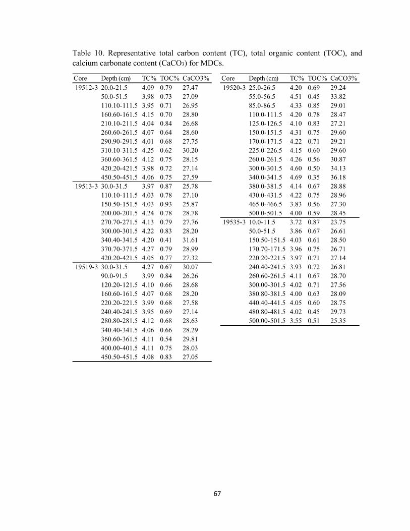
67  

Table 10. Representative total carbon content (TC), total organic content (TOC), and calcium carbonate content (CaCO3) for MDCs.

 

   

Core Depth (cm) TC% TOC% CaCO3% Core Depth (cm) TC% TOC% CaCO3%20.0-21.5 4.09 0.79 27.47 25.0-26.5 4.20 0.69 29.2450.0-51.5 3.98 0.73 27.09 55.0-56.5 4.51 0.45 33.82110.10-111.5 3.95 0.71 26.95 85.0-86.5 4.33 0.85 29.01160.60-161.5 4.15 0.70 28.80 110.0-111.5 4.20 0.78 28.47210.10-211.5 4.04 0.84 26.68 125.0-126.5 4.10 0.83 27.21260.60-261.5 4.07 0.64 28.60 150.0-151.5 4.31 0.75 29.60290.90-291.5 4.01 0.68 27.75 170.0-171.5 4.22 0.71 29.21310.10-311.5 4.25 0.62 30.20 225.0-226.5 4.15 0.60 29.60360.60-361.5 4.12 0.75 28.15 260.0-261.5 4.26 0.56 30.87420.20-421.5 3.98 0.72 27.14 300.0-301.5 4.60 0.50 34.13450.50-451.5 4.06 0.75 27.59 340.0-341.5 4.69 0.35 36.1830.0-31.5 3.97 0.87 25.78 380.0-381.5 4.14 0.67 28.88110.10-111.5 4.03 0.78 27.10 430.0-431.5 4.22 0.75 28.96150.50-151.5 4.03 0.93 25.87 465.0-466.5 3.83 0.56 27.30200.00-201.5 4.24 0.78 28.78 500.0-501.5 4.00 0.59 28.45270.70-271.5 4.13 0.79 27.76 10.0-11.5 3.72 0.87 23.75300.00-301.5 4.22 0.83 28.20 50.0-51.5 3.86 0.67 26.61340.40-341.5 4.20 0.41 31.61 150.50-151.5 4.03 0.61 28.50370.70-371.5 4.27 0.79 28.99 170.70-171.5 3.96 0.75 26.71420.20-421.5 4.05 0.77 27.32 220.20-221.5 3.97 0.71 27.1430.0-31.5 4.27 0.67 30.07 240.40-241.5 3.93 0.72 26.8190.0-91.5 3.99 0.84 26.26 260.60-261.5 4.11 0.67 28.70120.20-121.5 4.10 0.66 28.68 300.00-301.5 4.02 0.71 27.56160.60-161.5 4.07 0.68 28.20 380.80-381.5 4.00 0.63 28.09220.20-221.5 3.99 0.68 27.58 440.40-441.5 4.05 0.60 28.75240.40-241.5 3.95 0.69 27.14 480.80-481.5 4.02 0.45 29.73280.80-281.5 4.12 0.68 28.63 500.00-501.5 3.55 0.51 25.35340.40-341.5 4.06 0.66 28.29360.60-361.5 4.11 0.54 29.81400.00-401.5 4.11 0.75 28.03450.50-451.5 4.08 0.83 27.05

19512-3

19513-3

19519-3

19520-3

19535-3

 

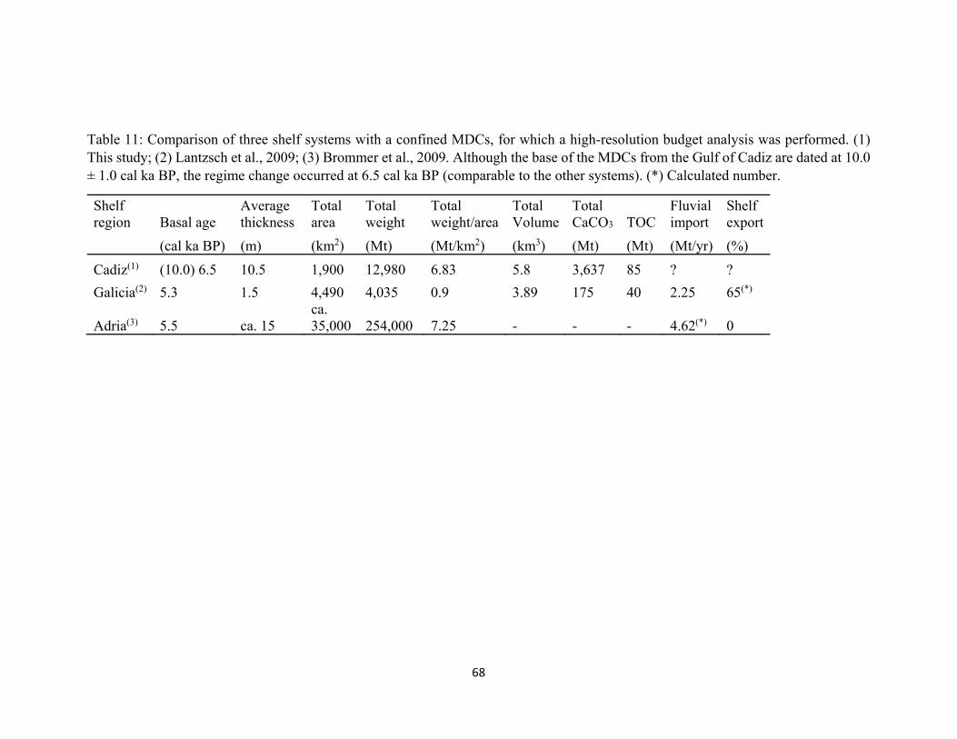
68  

Table 11: Comparison of three shelf systems with a confined MDCs, for which a high-resolution budget analysis was performed. (1) This study; (2) Lantzsch et al., 2009; (3) Brommer et al., 2009. Although the base of the MDCs from the Gulf of Cadiz are dated at 10.0 ± 1.0 cal ka BP, the regime change occurred at 6.5 cal ka BP (comparable to the other systems). (*) Calculated number.

Shelf region Basal age

Average thickness

Total area

Total weight

Total weight/area

Total Volume

Total CaCO3 TOC

Fluvial import

Shelf export

(cal ka BP) (m) (km2) (Mt) (Mt/km2) (km3) (Mt) (Mt) (Mt/yr) (%)

Cadiz(1) (10.0) 6.5 10.5 1,900 12,980 6.83 5.8 3,637 85 ? ?

Galicia(2) 5.3 1.5 4,490 4,035 0.9 3.89 175 40 2.25 65(*)

Adria(3) 5.5 ca. 15 ca. 35,000 254,000 7.25 - - - 4.62(*) 0

  

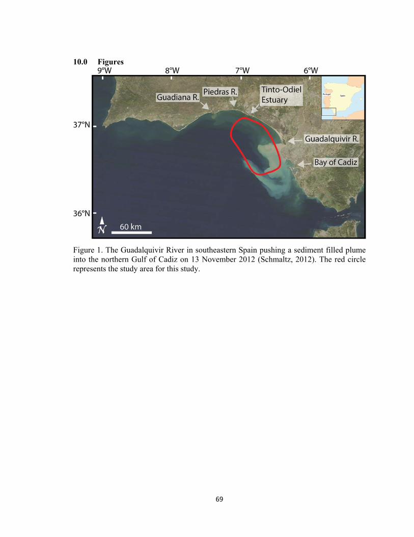
69  

10.0 Figures

Figure 1. The Guadalquivir River in southeastern Spain pushing a sediment filled plume into the northern Gulf of Cadiz on 13 November 2012 (Schmaltz, 2012). The red circle represents the study area for this study.

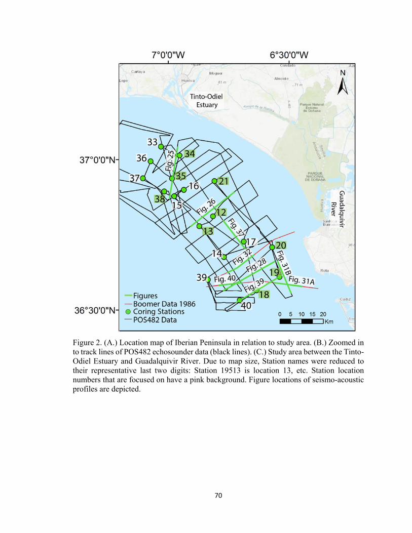
70  

Figure 2. (A.) Location map of Iberian Peninsula in relation to study area. (B.) Zoomed in to track lines of POS482 echosounder data (black lines). (C.) Study area between the Tinto-Odiel Estuary and Guadalquivir River. Due to map size, Station names were reduced to their representative last two digits: Station 19513 is location 13, etc. Station location numbers that are focused on have a pink background. Figure locations of seismo-acoustic profiles are depicted.

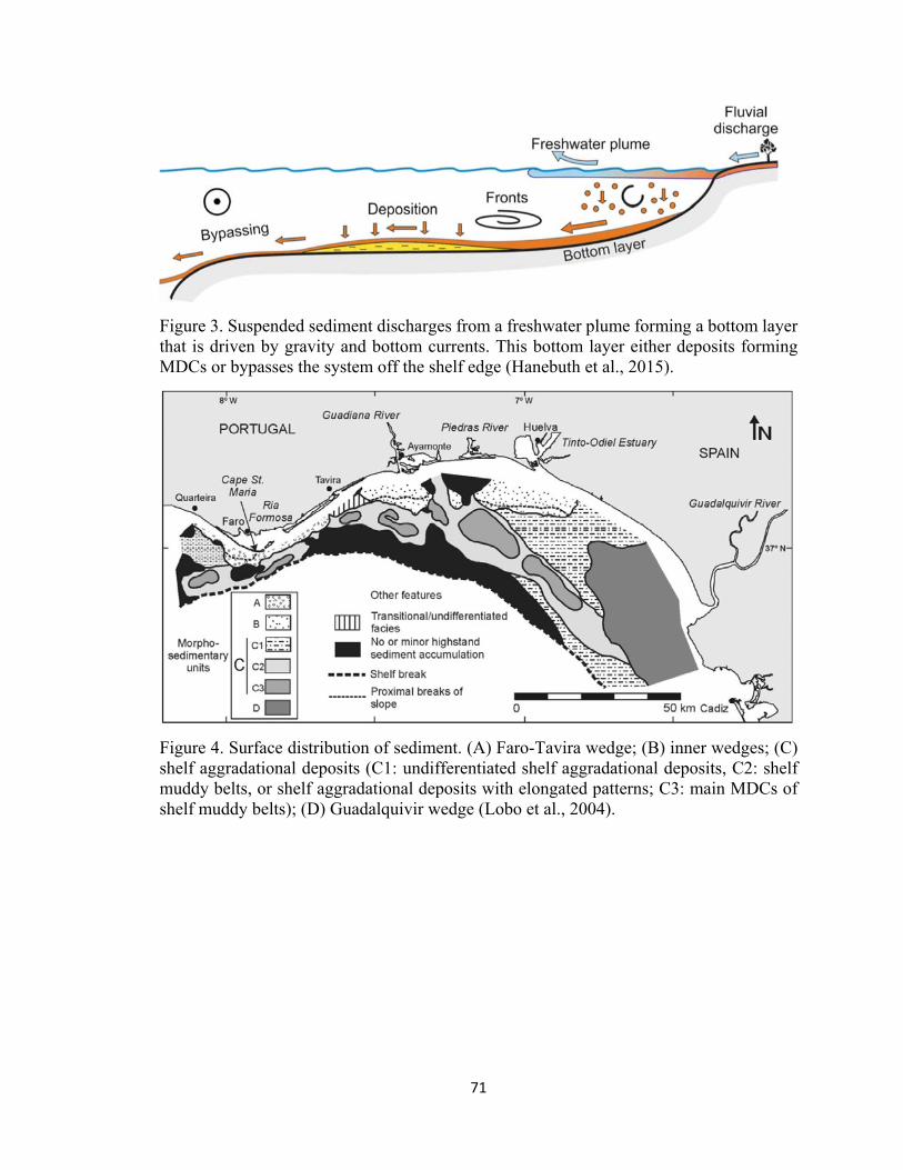
71  

Figure 3. Suspended sediment discharges from a freshwater plume forming a bottom layer that is driven by gravity and bottom currents. This bottom layer either deposits forming MDCs or bypasses the system off the shelf edge (Hanebuth et al., 2015).

Figure 4. Surface distribution of sediment. (A) Faro-Tavira wedge; (B) inner wedges; (C) shelf aggradational deposits (C1: undifferentiated shelf aggradational deposits, C2: shelf muddy belts, or shelf aggradational deposits with elongated patterns; C3: main MDCs of shelf muddy belts); (D) Guadalquivir wedge (Lobo et al., 2004).

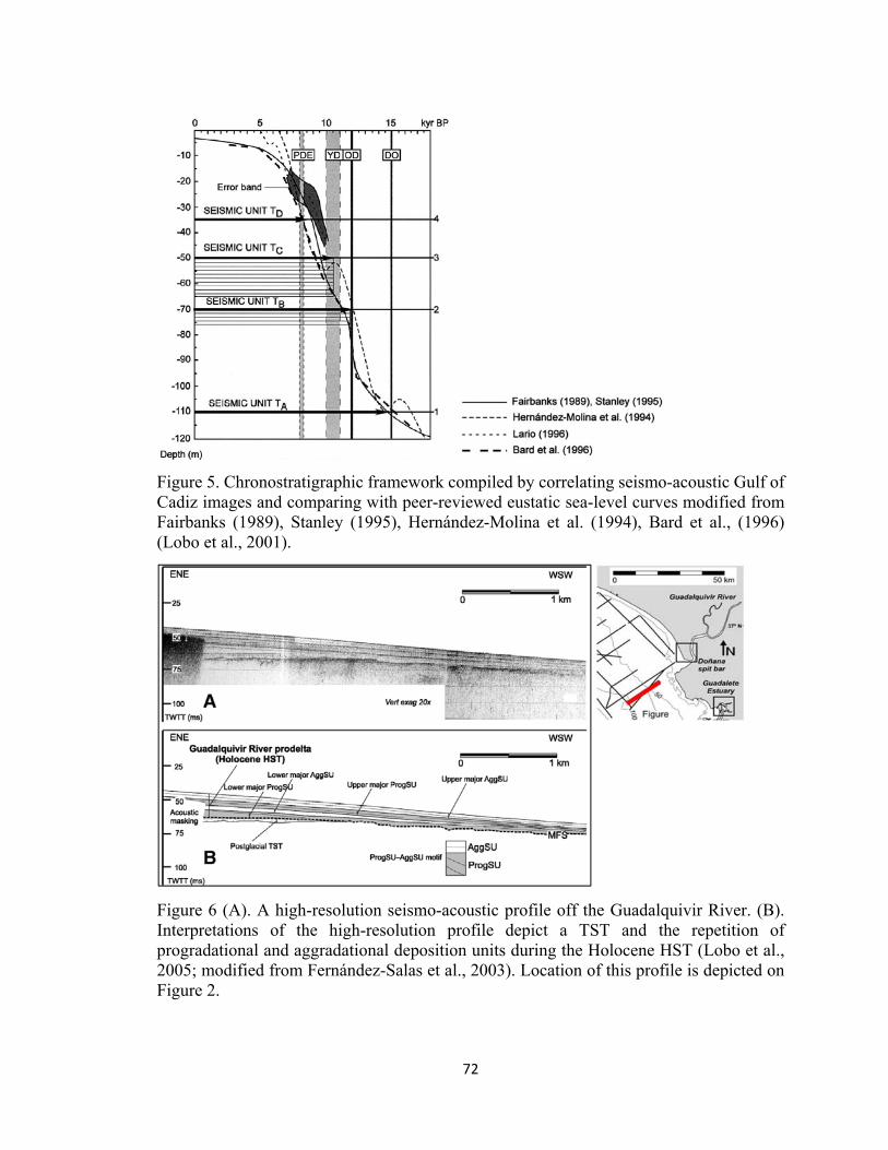
72  

Figure 5. Chronostratigraphic framework compiled by correlating seismo-acoustic Gulf of Cadiz images and comparing with peer-reviewed eustatic sea-level curves modified from Fairbanks (1989), Stanley (1995), Hernández-Molina et al. (1994), Bard et al., (1996) (Lobo et al., 2001).

Figure 6 (A). A high-resolution seismo-acoustic profile off the Guadalquivir River. (B). Interpretations of the high-resolution profile depict a TST and the repetition of progradational and aggradational deposition units during the Holocene HST (Lobo et al., 2005; modified from Fernández-Salas et al., 2003). Location of this profile is depicted on Figure 2.

 

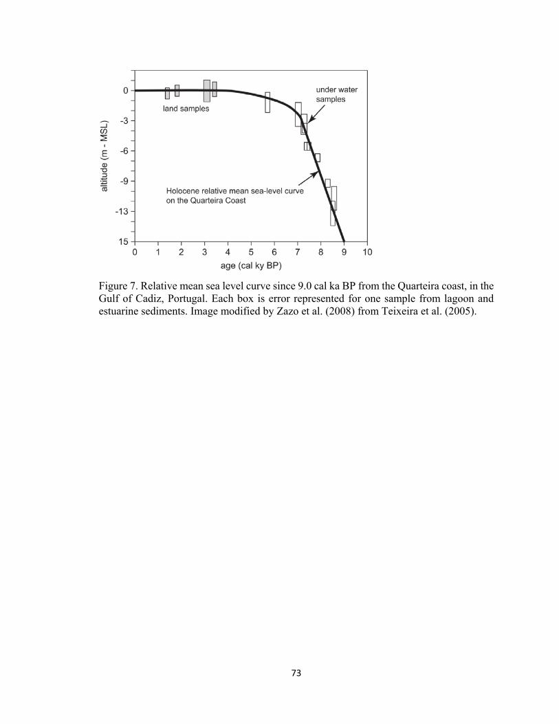
73  

Figure 7. Relative mean sea level curve since 9.0 cal ka BP from the Quarteira coast, in the Gulf of Cadiz, Portugal. Each box is error represented for one sample from lagoon and estuarine sediments. Image modified by Zazo et al. (2008) from Teixeira et al. (2005).

 

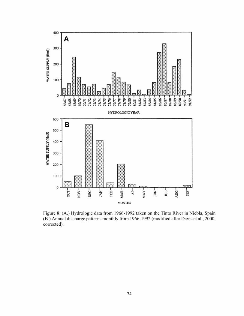
74  

Figure 8. (A.) Hydrologic data from 1966-1992 taken on the Tinto River in Niebla, Spain (B.) Annual discharge patterns monthly from 1966-1992 (modified after Davis et al., 2000, corrected).

 

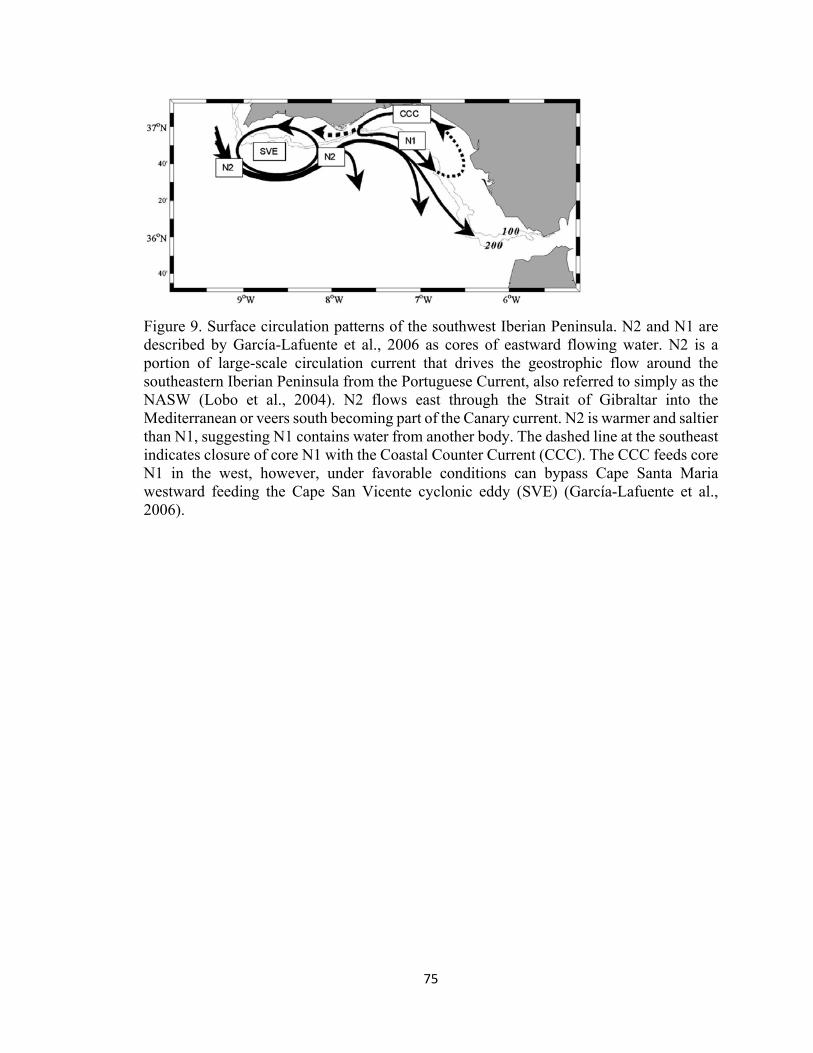
75  

Figure 9. Surface circulation patterns of the southwest Iberian Peninsula. N2 and N1 are described by García-Lafuente et al., 2006 as cores of eastward flowing water. N2 is a portion of large-scale circulation current that drives the geostrophic flow around the southeastern Iberian Peninsula from the Portuguese Current, also referred to simply as the NASW (Lobo et al., 2004). N2 flows east through the Strait of Gibraltar into the Mediterranean or veers south becoming part of the Canary current. N2 is warmer and saltier than N1, suggesting N1 contains water from another body. The dashed line at the southeast indicates closure of core N1 with the Coastal Counter Current (CCC). The CCC feeds core N1 in the west, however, under favorable conditions can bypass Cape Santa Maria westward feeding the Cape San Vicente cyclonic eddy (SVE) (García-Lafuente et al., 2006).

 

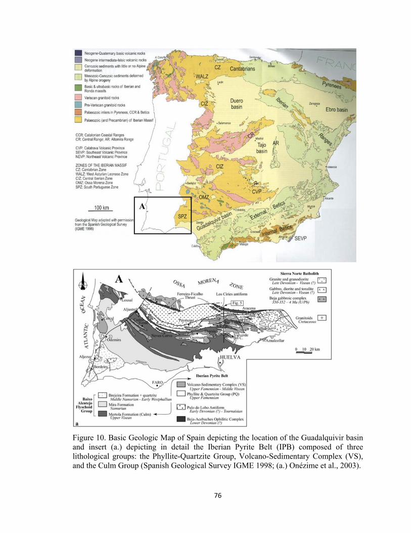
76  

Figure 10. Basic Geologic Map of Spain depicting the location of the Guadalquivir basin and insert (a.) depicting in detail the Iberian Pyrite Belt (IPB) composed of three lithological groups: the Phyllite-Quartzite Group, Volcano-Sedimentary Complex (VS), and the Culm Group (Spanish Geological Survey IGME 1998; (a.) Onézime et al., 2003).

 

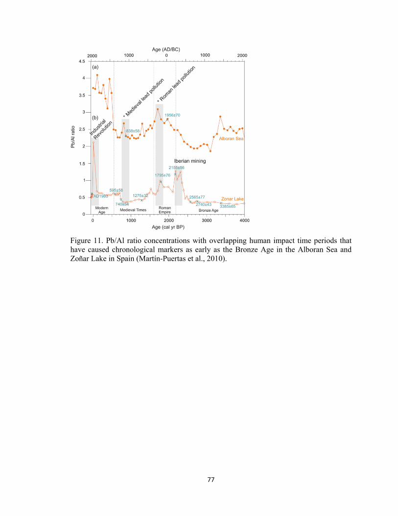
77  

Figure 11. Pb/Al ratio concentrations with overlapping human impact time periods that have caused chronological markers as early as the Bronze Age in the Alboran Sea and Zoñar Lake in Spain (Martín-Puertas et al., 2010).

 

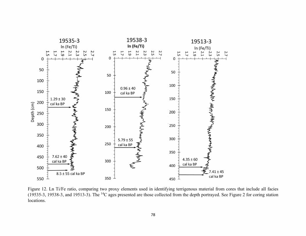
78  

Figure 12. Ln Ti/Fe ratio, comparing two proxy elements used in identifying terrigenous material from cores that include all facies (19535-3, 19538-3, and 19513-3). The 14C ages presented are those collected from the depth portrayed. See Figure 2 for coring station locations.

19535‐3  19538‐3 19513‐3

 

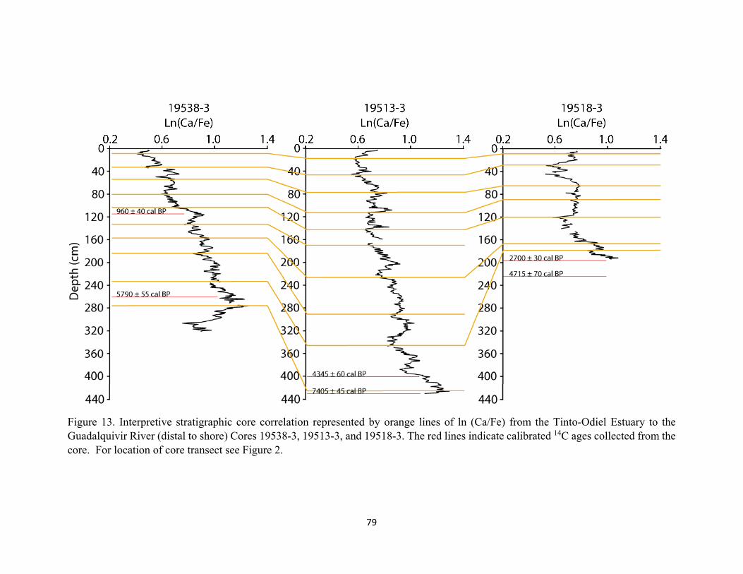
79  

Figure 13. Interpretive stratigraphic core correlation represented by orange lines of ln (Ca/Fe) from the Tinto-Odiel Estuary to the Guadalquivir River (distal to shore) Cores 19538-3, 19513-3, and 19518-3. The red lines indicate calibrated 14C ages collected from the core. For location of core transect see Figure 2.

 

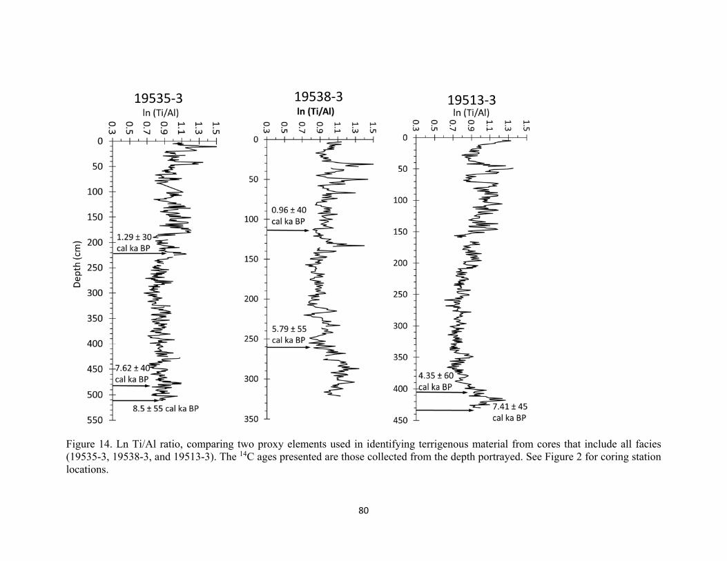
80  

Figure 14. Ln Ti/Al ratio, comparing two proxy elements used in identifying terrigenous material from cores that include all facies (19535-3, 19538-3, and 19513-3). The 14C ages presented are those collected from the depth portrayed. See Figure 2 for coring station locations.

19535‐3  19538‐3 19513‐3

 

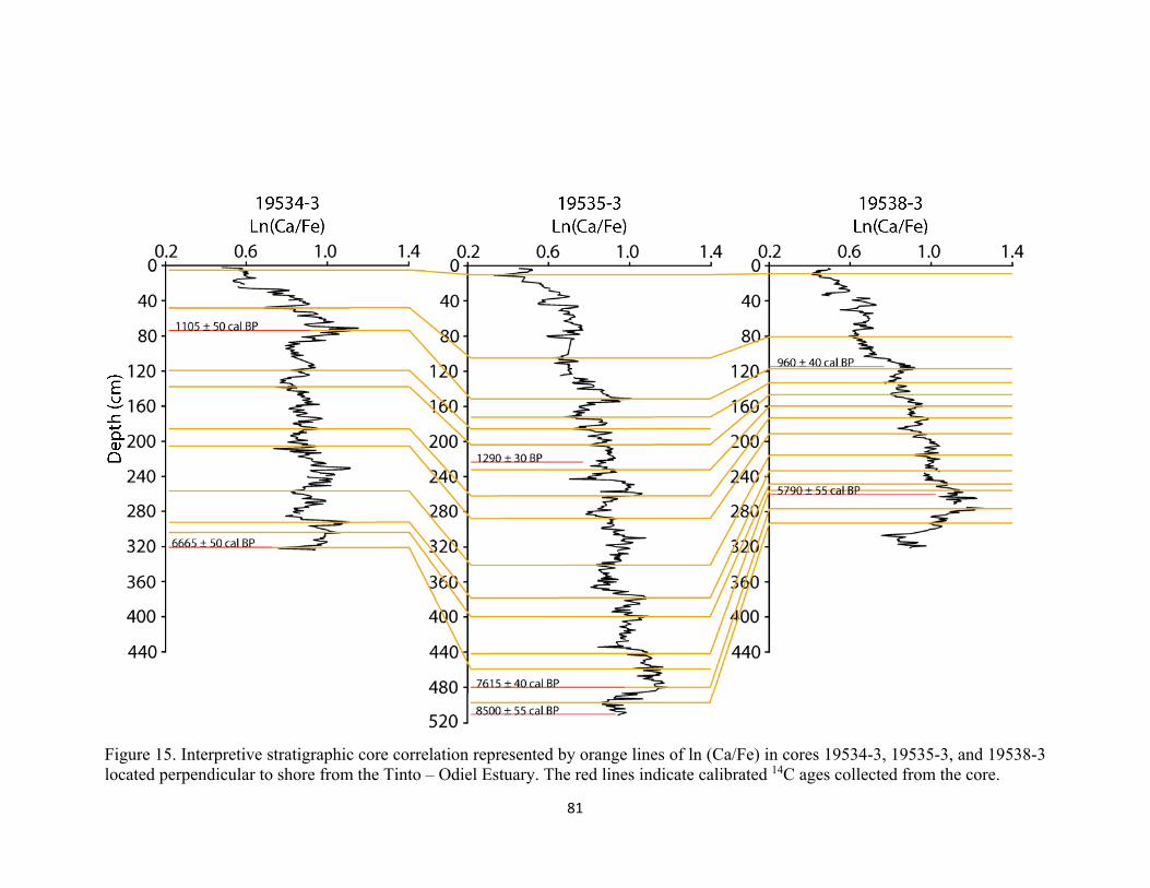
81  

Figure 15. Interpretive stratigraphic core correlation represented by orange lines of ln (Ca/Fe) in cores 19534-3, 19535-3, and 19538-3 located perpendicular to shore from the Tinto – Odiel Estuary. The red lines indicate calibrated 14C ages collected from the core.

 

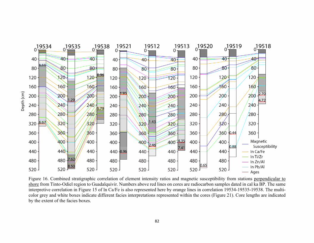
82  

Figure 16. Combined stratigraphic correlation of element intensity ratios and magnetic susceptibility from stations perpendicular to shore from Tinto-Odiel region to Guadalquivir. Numbers above red lines on cores are radiocarbon samples dated in cal ka BP. The same interpretive correlation in Figure 15 of ln Ca/Fe is also represented here by orange lines in correlation 19534-19535-19538. The multi-color grey and white boxes indicate different facies interpretations represented within the cores (Figure 21). Core lengths are indicated by the extent of the facies boxes.

Dep

th (cm

) 

 

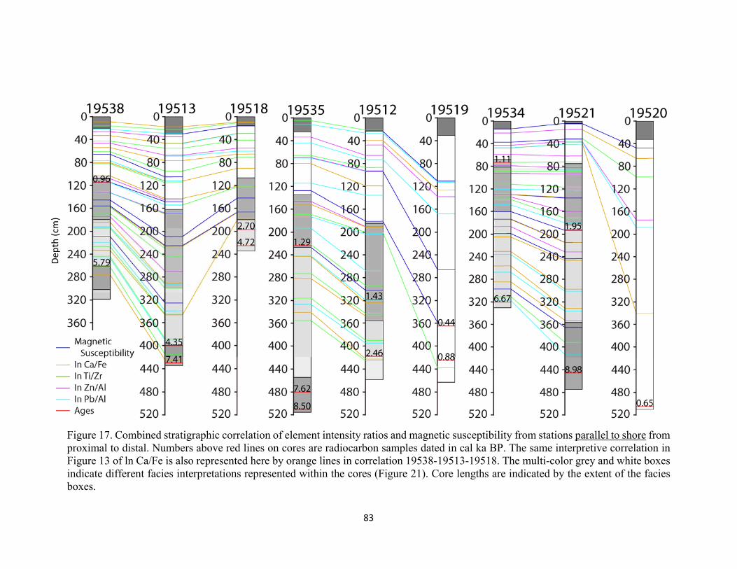
83  

Figure 17. Combined stratigraphic correlation of element intensity ratios and magnetic susceptibility from stations parallel to shore from proximal to distal. Numbers above red lines on cores are radiocarbon samples dated in cal ka BP. The same interpretive correlation in Figure 13 of ln Ca/Fe is also represented here by orange lines in correlation 19538-19513-19518. The multi-color grey and white boxes indicate different facies interpretations represented within the cores (Figure 21). Core lengths are indicated by the extent of the facies boxes.

Dep

th (cm

) 

 

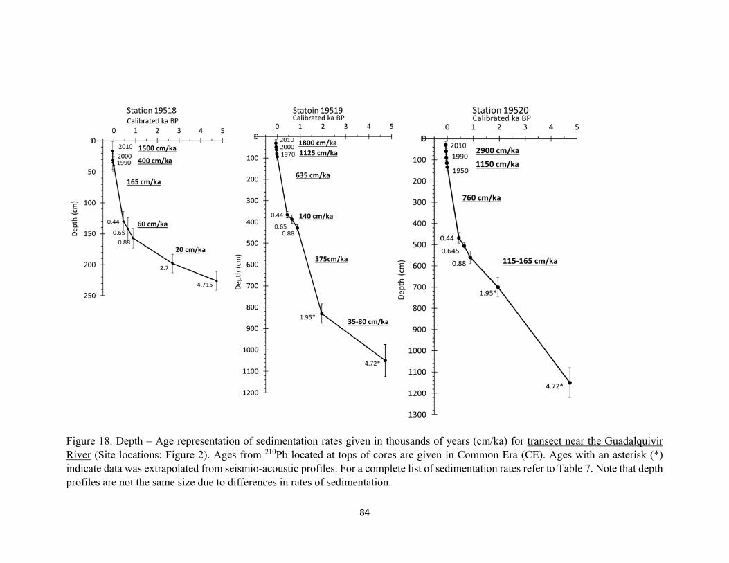
84  

Figure 18. Depth – Age representation of sedimentation rates given in thousands of years (cm/ka) for transect near the Guadalquivir River (Site locations: Figure 2). Ages from 210Pb located at tops of cores are given in Common Era (CE). Ages with an asterisk (*) indicate data was extrapolated from seismio-acoustic profiles. For a complete list of sedimentation rates refer to Table 7. Note that depth profiles are not the same size due to differences in rates of sedimentation.

 

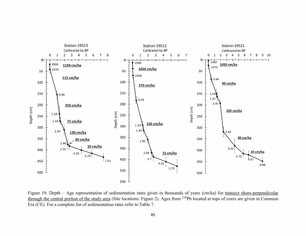
85  

Figure 19. Depth – Age representation of sedimentation rates given in thousands of years (cm/ka) for transect shore-perpendicular through the central portion of the study area (Site locations: Figure 2). Ages from 210Pb located at tops of cores are given in Common Era (CE). For a complete list of sedimentation rates refer to Table 7.

 

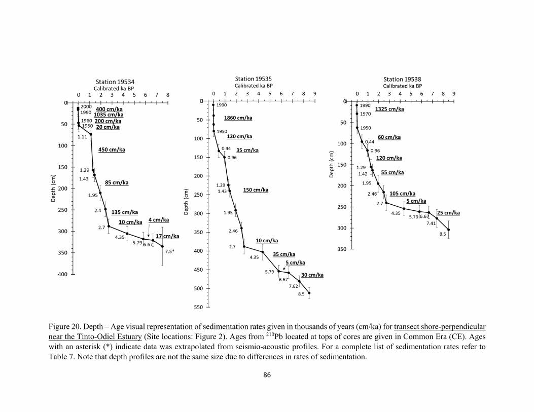
86  

Figure 20. Depth – Age visual representation of sedimentation rates given in thousands of years (cm/ka) for transect shore-perpendicular near the Tinto-Odiel Estuary (Site locations: Figure 2). Ages from 210Pb located at tops of cores are given in Common Era (CE). Ages with an asterisk (*) indicate data was extrapolated from seismio-acoustic profiles. For a complete list of sedimentation rates refer to Table 7. Note that depth profiles are not the same size due to differences in rates of sedimentation.

 

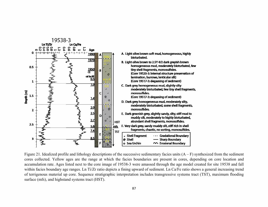
87  

Figure 21. Idealized profile and lithology descriptions of the successive sedimentary facies units (A – F) synthesized from the sediment cores collected. Yellow ages are the range at which the facies boundaries are present in cores, depending on core location and accumulation rate. Ages listed next to the core image of 19538-3 were amassed through the age model created for site 19538 and fall within facies boundary age ranges. Ln Ti/Zr ratio depicts a fining upward of sediment. Ln Ca/Fe ratio shows a general increasing trend of terrigenous material up core. Sequence stratigraphic interpretation includes transgressive systems tract (TST), maximum flooding surface (mfs), and highstand systems tract (HST).

 

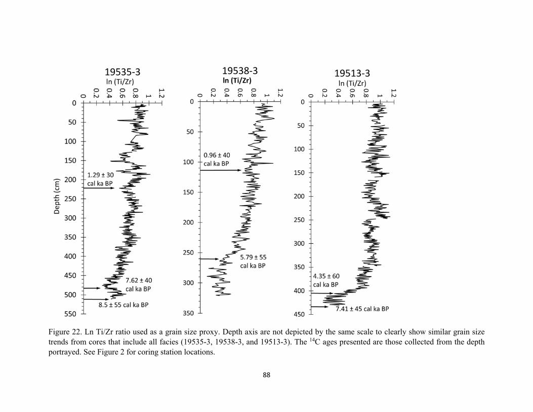
88  

Figure 22. Ln Ti/Zr ratio used as a grain size proxy. Depth axis are not depicted by the same scale to clearly show similar grain size trends from cores that include all facies (19535-3, 19538-3, and 19513-3). The 14C ages presented are those collected from the depth portrayed. See Figure 2 for coring station locations.

19535‐3  19538‐3 19513‐3

 

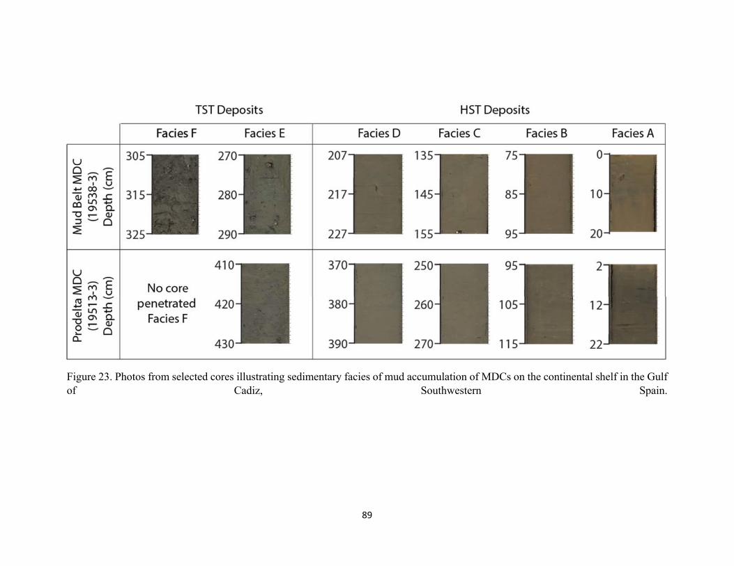
89  

Figure 23. Photos from selected cores illustrating sedimentary facies of mud accumulation of MDCs on the continental shelf in the Gulf of Cadiz, Southwestern Spain.

 

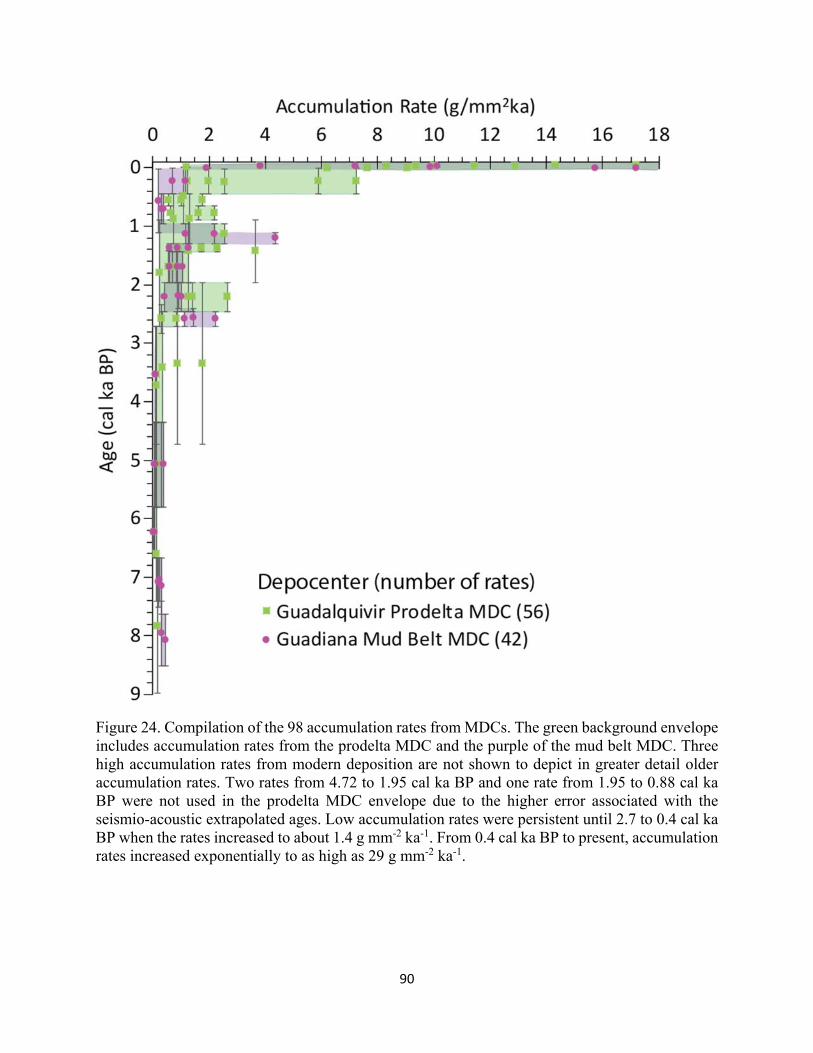
90  

Figure 24. Compilation of the 98 accumulation rates from MDCs. The green background envelope includes accumulation rates from the prodelta MDC and the purple of the mud belt MDC. Three high accumulation rates from modern deposition are not shown to depict in greater detail older accumulation rates. Two rates from 4.72 to 1.95 cal ka BP and one rate from 1.95 to 0.88 cal ka BP were not used in the prodelta MDC envelope due to the higher error associated with the seismio-acoustic extrapolated ages. Low accumulation rates were persistent until 2.7 to 0.4 cal ka BP when the rates increased to about 1.4 g mm-2 ka-1. From 0.4 cal ka BP to present, accumulation rates increased exponentially to as high as 29 g mm-2 ka-1.

 

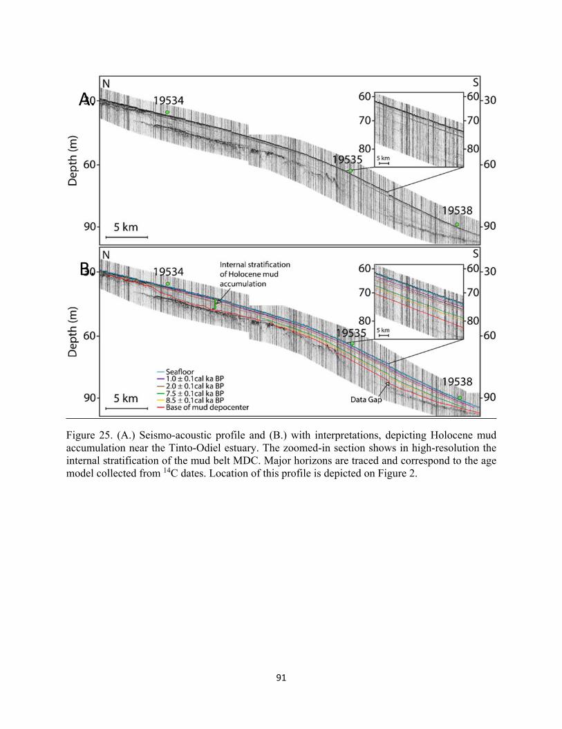
91  

Figure 25. (A.) Seismo-acoustic profile and (B.) with interpretations, depicting Holocene mud accumulation near the Tinto-Odiel estuary. The zoomed-in section shows in high-resolution the internal stratification of the mud belt MDC. Major horizons are traced and correspond to the age model collected from 14C dates. Location of this profile is depicted on Figure 2.

A. 

B. 

 

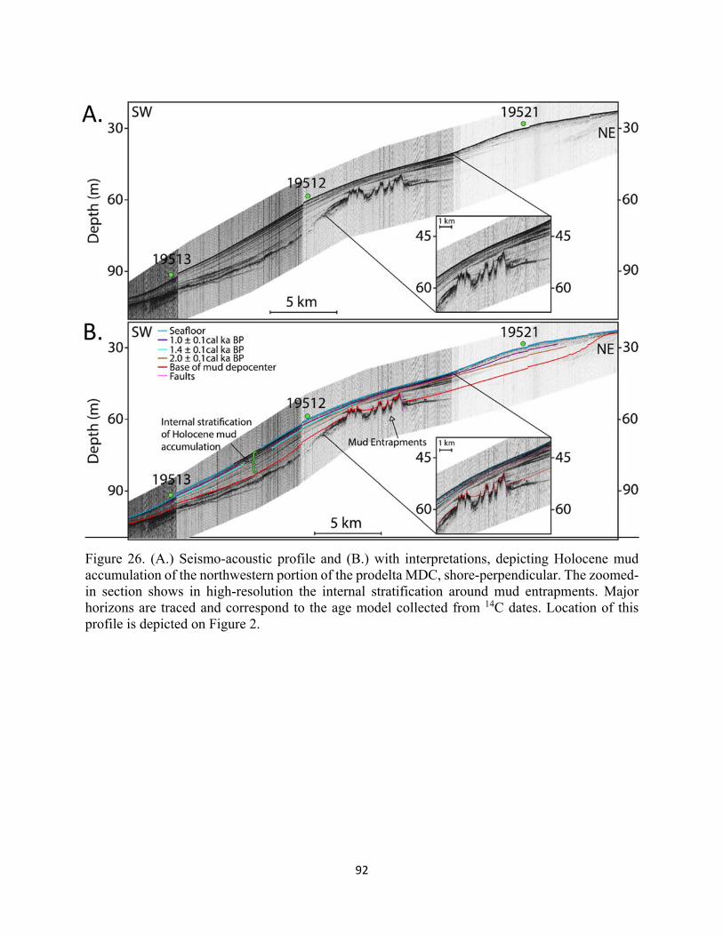
92  

Figure 26. (A.) Seismo-acoustic profile and (B.) with interpretations, depicting Holocene mud accumulation of the northwestern portion of the prodelta MDC, shore-perpendicular. The zoomed-in section shows in high-resolution the internal stratification around mud entrapments. Major horizons are traced and correspond to the age model collected from 14C dates. Location of this profile is depicted on Figure 2.

A. 

B. 

 

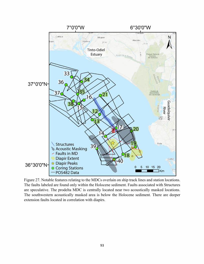
93  

Figure 27. Notable features relating to the MDCs overlain on ship track lines and station locations. The faults labeled are found only within the Holocene sediment. Faults associated with Structures are speculative. The prodelta MDC is centrally located near two acoustically masked locations. The southwestern acoustically masked area is below the Holocene sediment. There are deeper extension faults located in correlation with diapirs.

 

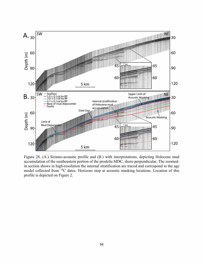
94  

Figure 28. (A.) Seismo-acoustic profile and (B.) with interpretations, depicting Holocene mud accumulation of the southeastern portion of the prodelta MDC, shore-perpendicular. The zoomed-in section shows in high-resolution the internal stratification are traced and correspond to the age model collected from 14C dates. Horizons stop at acoustic masking locations. Location of this profile is depicted on Figure 2.

A. 

B. 

 

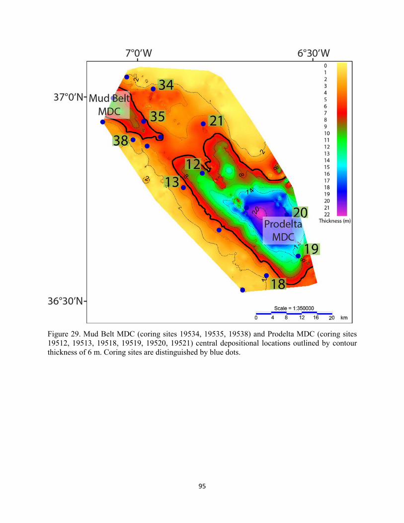
95  

Figure 29. Mud Belt MDC (coring sites 19534, 19535, 19538) and Prodelta MDC (coring sites 19512, 19513, 19518, 19519, 19520, 19521) central depositional locations outlined by contour thickness of 6 m. Coring sites are distinguished by blue dots.

 

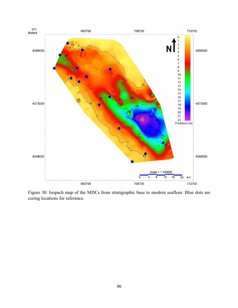
96  

Figure 30. Isopach map of the MDCs from stratigraphic base to modern seafloor. Blue dots are coring locations for reference.    

 

97  

Figure 31. (Profile A) One lobe of the eastern diapiric uplift, close to the Guadalquivir River, 40 m from mean sea level. (Profile B) The cap rock of the diapir has penetrated the base of the prodelta MDC, 3 m from seafloor. Location of seismio-acoustic profiles in Figure 2.

 

98  

Figure 32. Western diapir with related extension faults, located near shelf edge below the base of the prodelta MDC. Location of seismio-acoustic profile in Figure 2.

 

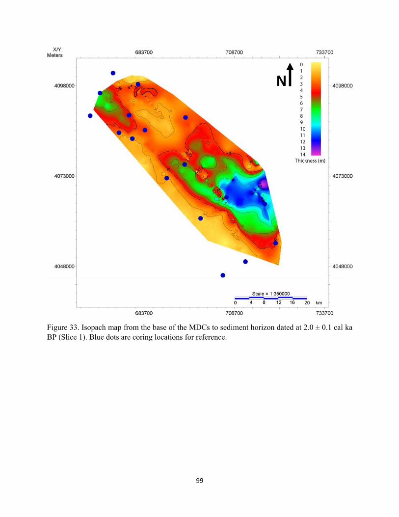
99  

Figure 33. Isopach map from the base of the MDCs to sediment horizon dated at 2.0 ± 0.1 cal ka BP (Slice 1). Blue dots are coring locations for reference.

 

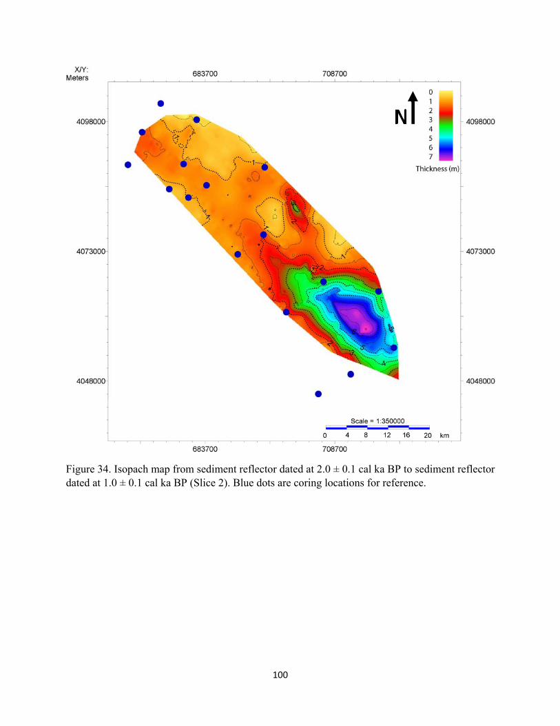
100  

Figure 34. Isopach map from sediment reflector dated at 2.0 ± 0.1 cal ka BP to sediment reflector dated at 1.0 ± 0.1 cal ka BP (Slice 2). Blue dots are coring locations for reference.

 

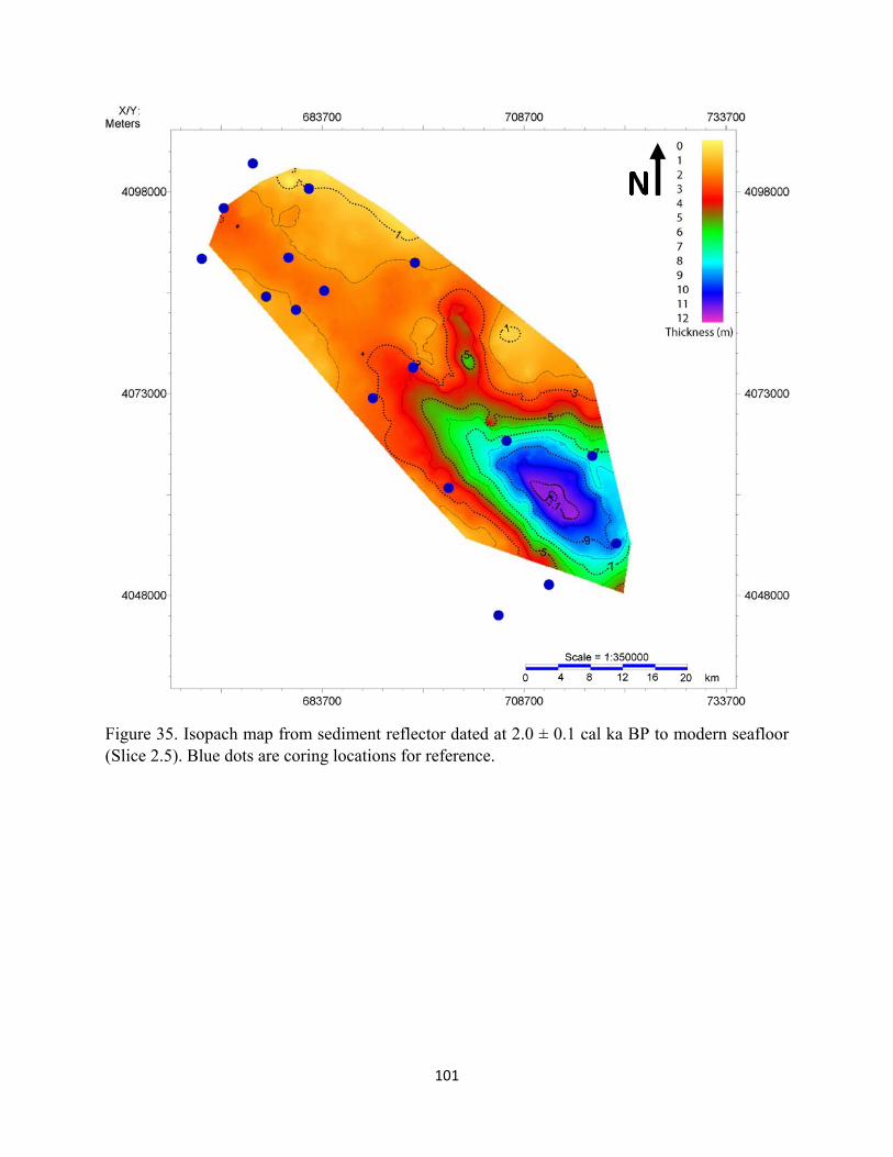
101  

Figure 35. Isopach map from sediment reflector dated at 2.0 ± 0.1 cal ka BP to modern seafloor (Slice 2.5). Blue dots are coring locations for reference.

 

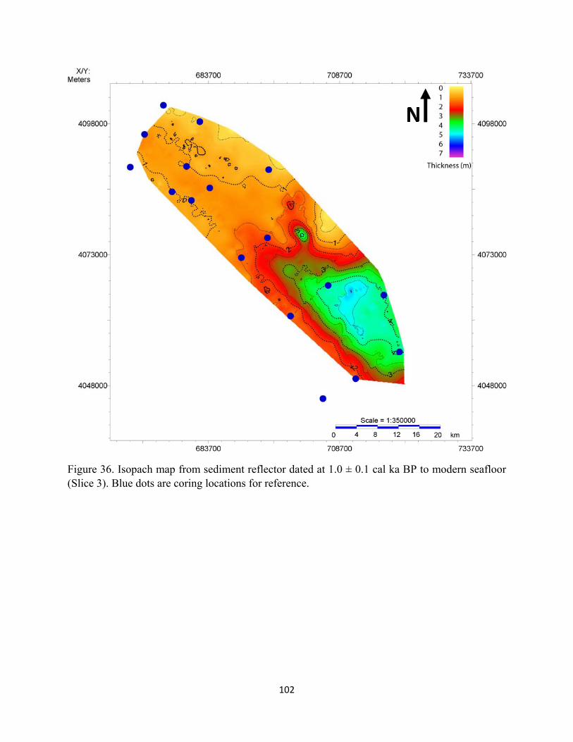
102  

Figure 36. Isopach map from sediment reflector dated at 1.0 ± 0.1 cal ka BP to modern seafloor (Slice 3). Blue dots are coring locations for reference.

 

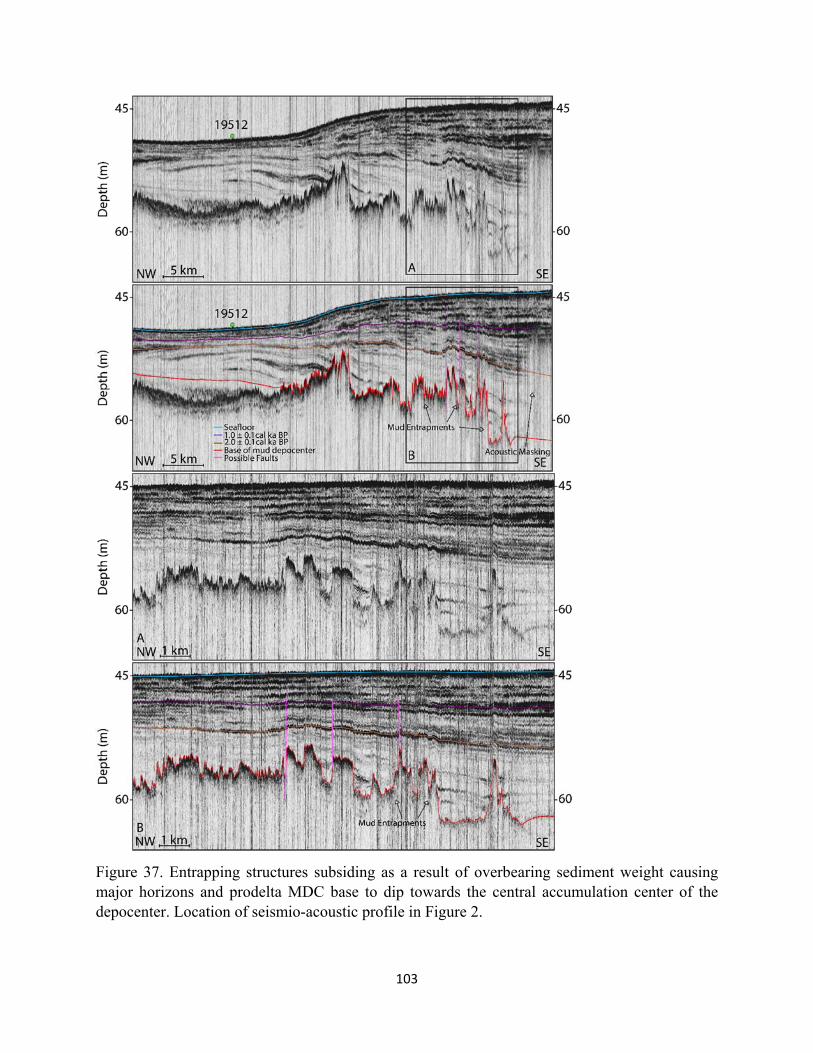
103  

Figure 37. Entrapping structures subsiding as a result of overbearing sediment weight causing major horizons and prodelta MDC base to dip towards the central accumulation center of the depocenter. Location of seismio-acoustic profile in Figure 2.

 

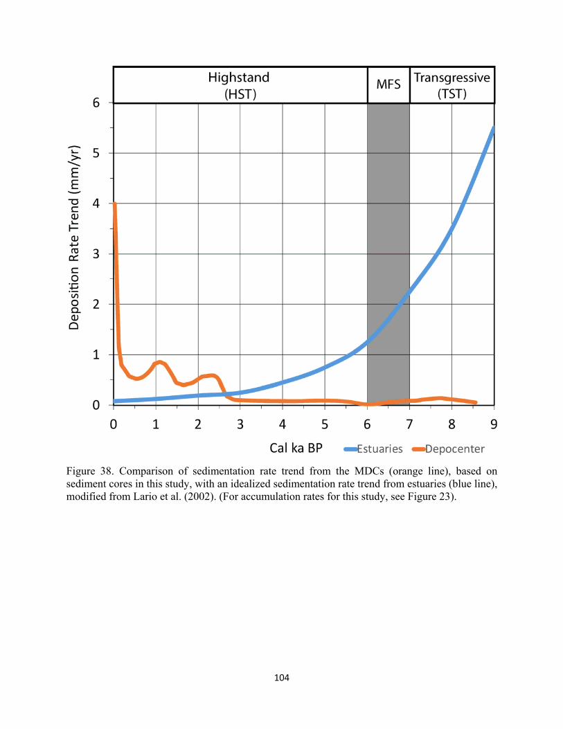
104  

Figure 38. Comparison of sedimentation rate trend from the MDCs (orange line), based on sediment cores in this study, with an idealized sedimentation rate trend from estuaries (blue line), modified from Lario et al. (2002). (For accumulation rates for this study, see Figure 23).

 

105  

Figure 39. Evidence of block-like subsidence occurring between the two main diapir locations affecting the prodelta MDC. Location of seismio-acoustic profile in Figure 2.

 

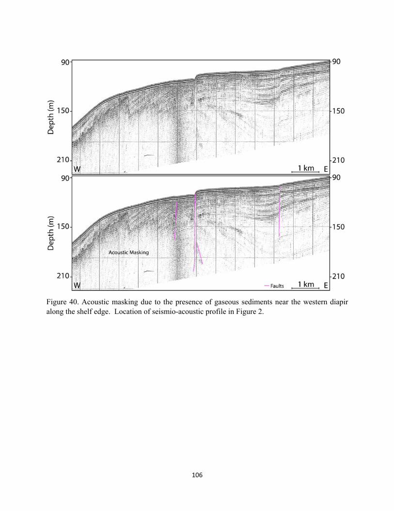
106  

Figure 40. Acoustic masking due to the presence of gaseous sediments near the western diapir along the shelf edge. Location of seismio-acoustic profile in Figure 2.

107  

11.0 References Abrantes, F., Rodrigues, T., Rufino, M., Salgueiro, E., Oliveira, D., Gomes, S., Oliveira,

P., Costa, A., Mil-Homens, M., Drago, T., Naughton, F. (2017) The climate of the Common Era off the Iberian Peninsula. Climate of the Past 13: 1901-1918.

Alley, R.B., Mayewski, P.A., Sowers, T., Stuiver, M., Taylor, K.C., Clark, P.U. (1997) Holocene climatic instability: A prominent, widespread event 8200 yr ago. Geology 25 (6): 483-486.

Alves, M., Gaillard, F., Sparrow, M., Knoll, M., Giraud, S. (2002) Circulation patterns and transport of the Azores Front-Current system. Deep-Sea Research II 49: 3983-4002.

Appleby, P.G., Oldfield, F. (1978) The calculation of lead-210 dates assuming a constant rate of supply of unsupported 210Pb to the sediment. Catena 5: 1–8.

Baptista, M.A., Miranda, P., Luis, J.F. (2006) In search of the 31 March 1761 earthquake and tsunami source. Bulletin of the Seismological Society of America 96(2): 713-721.

Baptista, M.A., Miranda, P., Victor, L.M. (1992) Maximum Entropy Analysis of Portuguese Tsunami Data te Tsunamis of 28.02.1969 and 26.05.1975. Science Of Tsunami Hazards 10: 9-20.

Bard, E., Hamelin, B., Arnold, M., Montaggioni, L., Cabiochll, G., Faure, G., Rougerie, F. (1996) Deglacial sea-level record from Tahiti corals and the timing of global meltwater discharge. Nature 382: 241-244.

Baringer, M.O. and J. F. Price (1999) A review of the physical oceanography of the Mediterranean outflow. Marine Geology 155: 63-82.

Barrie, C.T. and Hannington, M.D. (1999) Classification of Volcanic-Associated Massive Sulfide Deposits Based on Host-Rock Composition. Reviews in Economic Geology 8: 1-11.

Bird, M.I., Fifield, L.K., Teh, T.S., Chang, C.H., Shirlaw, N., Lambeck, K. (2007) An inflection in the rate of early mid-Holocene eustatic sea-level rise: A new sea-level curve from Singapore. Estuarine, Coastal and Shelf Science 71: 523-536.

Bond, G., Kromer, B., Beer, J., Muscheler, R., Evans, M.N., Showers, W., Hoffmann, S., Lotti-Bond, R., Hajdas, I., Bonani, G. (2001) Persistent Solar Influence on North Atlantic Climate during the Holocene. Science. 294: 2130-2136.

Bond, G., Showers, W., Cheseby, M., Lotti, R., Almasi, P., DeMenocal, P., Priore, P., Cullen, H., Hajdas, I., Bonani, G. (1997) A Pervasive Millennial-Scale Cycle in North Atlantic Holocene and Glacial Climates. Science 278: 1257-1266.

Borrego, J., Morales, J.A., Pendón, J.G. (1993) Holocene Filling of an Estuarine Lagoon along the Mesotidal Coast of Huelva: The Piedras River Mouth, Southwestern Spain. Journal of Coastal Research 9 (1): 242-254.

Brommer, M.B.,Weltje, G.J., Trincardi, F. (2009) Reconstruction of sediment supply from mass accumulation rates in the Northern Adriatic Basin (Italy) over the past 19,000 years. Journal of Geophysical Research 114: 1-15.

Cáceres, L.M., Olías, M., De Andrés, J.R., Rodríguez-Vidal, J., Clemente, L., Galván, L., Medina, B. (2013) Geochemistry of Quaternary sediments in terraces of the Tinto River (SW Spain): Paleoenvironmental implications. Catena 101: 1-10.

Casas, D., Ercilla, G., Baraza, J. (2003) Acoustic evidence of gas in the continental slope sediments of the Gulf of Cadiz (E Atlantic). Geo-Marine Letters 23: 300-310.

108  

Cherubin, L. M., Carton, X., Paillet, J., Morel, Y., Serpette, A. (2000) Instability of the Mediterranean Water undercurrents southwest of Portugal: Effects of baroclinity and of topography. Oceanologica Acta 23: 551-574.

Criado-Aldeanueva, F., García-Lafuente, J., Vargas, J.M., Del Rıó, J., Sánchez, A. Delgado, J., Sánchez, J. C. (2006a) Wind induced variability of hydrographic features and water masses distribution in the Gulf of Cadiz (SW Iberia) from in situ data. Journal of Marine Systems 63: 130-140.

Criado-Aldeanueva, F., García-Lafuente, J., Vargas, J.M., Del Rıó, J., Vaquez, A., Reul, A., Sánchez, A. (2006b) Distribution and circulation of water masses in the Gulf of Cadiz from in situ observations. Deep-Sea Research II 53: 1144-1160.

Cruise Report POS482. RV Poseidon. Lantzsch, H., Hanebuth, T.J.J., Bergmann, F., Kestner, M., King, M.L., Lobo, F.J., Luján, M., Mendes, I., Reguera, I., Schwenk, T., Steinborn, B., Warratz, G. Confined transgressive and highstand sediment depocenters in the Gulf of Cadiz: reconstruction of formation history and past environmental changes. March 14 – 25, 2015 Portimão, Portugal – Málaga, Spain. Cadiz Shelf Sediment Depocenters (CADISED). (http://oceanrep.geomar.de/28929/).

Currie, Lloyd A. (2004) The remarkable metrological history of radiocarbon dating [II]. Journal of Research of the National Institute of Standards and Technology 109: 185-217.

Darby, D.A., Ortiz, J.D., Grosch, C.E., Lund, S.P. (2012) 1,500-year cycle in the Arctic Oscillation identified in Holocene Arctic sea-ice drift. Nature Geoscience 5: 897-900.

Davis Jr., R., Welty, A., Borrego, J. Morales, J.A., Ryan, J.G. (2000) Rio Tinto estuary (Spain): 5000 years of pollution. Environmental Geology 39: 1107-1116.

Delgado, J., Boski, T., Nieto, J. M., Pereira, L., Moura, D., Gomes, A., Sousa, C., García-Tenorio, R. (2012) Sea-level rise and anthropogenic activities recorded in the late Pleistocene / Holocene sedimentary infill of the Guadiana Estuary (SW Iberia). Quaternary Science Reviews 33: 121-141.

Fairbanks, R.G. (1989) A 17,000-year glacio-eustatic sea level record: influence of glacial melting rates on the Younger Dryas event and deep-ocean circulation. Nature 342: 637-642.

Fanget, A.S., Berné, S., Jouet, G., Bassetti, M.A., Dennielou, B., Maillet, G.M., Tondut, M. (2014) Impact of relative sea level and rapid climate changes on the architecture and lithofacies of the Holocene Rhone subaqueous delta (Western Mediterranean Sea). Sedimentary Geology 305: 35-53.

Fernández-Puga, M.C., Vázquez, J.T., Somoza, L., Díaz del Rio, V., Medialdea, T., Mata, M.P., León, R. (2007) Gas-related morphologies and diapirism in the Gulf of Cádiz. Geo-Marine Letters 27: 213-221.

Fernández-Salas, L.M., Lobo, F.J., Hernández-Molina, F.J., Somoza, L., Rodero, J., Díaz Del Río, V., Maldonado, A. (2003) High-resolution architecture of late Holocene highstand prodeltaic deposits from southern Spain: the imprint of high-frequency climatic and relative sea-level changes. Continental Shelf Research 23: 1037-1054.

Galbis, R.J. (1932) Catálogo sísmico de la zona comprendida entre los meridianos 58E y 208W de Greenwich y los paralelos 45º y 25º N. Dirección General del Instituto Geográfico, Catastral y de Estadística, Madrid.

109  

García-Lafuente, J., Delgado, J., Criado-Aldeanueva, F., Bruno, M., Del Rıó, J., Vargas, J.M. (2006) Water mass circulation on the continental shelf of the Gulf of Cadiz. Deep-Sea Research II 53: 1182-1197.

Garel, E., Laiz, I., Drago, T., Relvas, P. (2016) Characterization of coastal counter-currents on the inner shelf of the Gulf of Cadiz. Journal of Marine Systems 155: 19-34.

González-Ortegón, E., Subida, M.D., Cuesta, J.A., Arias, A.M., Fernández-Delgado, C., Drake, P. (2010) The impact of extreme turbidity events on the nursery function of a temperate European estuary with regulated freshwater inflow. Estuarine, Coastal and Shelf Science 87: 311-324.

Goy, J.L., Zazo, C., Dabrio, C.J., Lario, J., Borja, F., Sierro, F.J., Flores, J.A. (1996) Global and regional factors controlling changes of coastlines in Southern Iberia (Spain) during the Holocene. Quaternary Science Reviews 15 (8-9): 773-780.

Hanebuth, T.J.J. and Henrich, R. (2009) Recurrent decadal-scale dust events over Holocene western Africa and their control on canyon turbidite activity (Mauritania). Quaternary Science Reviews 28: 261-270.

Hanebuth, T.J.J., Lantzsch, H., Nizou, J. (2015a) Mud depocenters on continental shelves—appearance, initiation times, and growth dynamics. Geo-Mar Lett 35: 487-503.

Hanebuth, T.J.J., Zhang, W., Hofmann, A.L., Lӧwemark, L.A., Schwenk, T. (2015b) Oceanic density fronts steering bottom-current induced sedimentation deduced from a 50 ka contourite-drift record and numerical modeling (off NW Spain). Quaternary Science Reviews 112: 207-225.

Hanebuth, T.J.J., King, M.L., Mendes, I., Lebreiro, S., Lobo, F.J., Oberle, F. K.J., Antón, L., Ferreira, P.A., Reguera, M.I. (2018) Hazard potential of widespread but hidden historic offshore heavy metal (Pb, Zn) contamination (Gulf of Cadiz, Spain). Science of the Total Environment 637-638: 561-576.

Hanebuth, T.J.J., Voris, H.K., Yokoyama, Y., Saito, Y., Okuno, J. (2011) Formation and fate of sedimentary depocentres on Southeast Asia's Sunda Shelf over the past sea-level cycle and biogeographic implications. Earth-Science Reviews 104: 92-110.

Hanquiez, V., Mulder, T., Lecroart, P., Gonthier, E., Marchès, E., Voisset, M. (2007) High resolution seafloor images in the Gulf of Cadiz, Iberian margin. Marine Geology 246: 42-59.

Hernández-Molina, F.J., Somoza, L., Lobo, F.J. (2000) Seismic stratigraphy of the Gulf of Cádiz continental shelf: a model for Late Quaternary very high-resolution sequence stratigraphy and response to sea-level fall. In: Hunt D, Gawthorpe RLG (eds) Sedimentary responses to forced regressions. Geological Society Special Publication 172: 329–361.

Hernández-Molina, F.J., Somoza, L., Rey, J., Pomar, L. (1994) Late Pleistocene – Holocene sediments on the Spanish continental shelves: Model for very high resolution sequence stratigraphy. Marine Geology 120: 129–174.

Hill, P.S., Fox, J.M., Crockett, J.S., Curran, K.J., Friedrichs, C.T., Geyer, W.R., Milligan, T.G., Ogston, A.S., Puig, P., Scully, M.E., Traykovski, P.A., Wheatcroft, R.A. (2007) Sediment delivery to the seabed on continental margins. Special Publication of the International Association of Sedimentologists 37: 49-99.

Jiménez-Moreno, G., Rodríguez-Ramírez, A., Pérez-Asensio, J.N., Carrión, J.S., López-Sáez, J.A., Villarías-Robles, J.J.R., Celestino-Pérez, S., Cerrillo-Cuenca, E., León,

110  

Á., Contreras, C. (2015) Impact of late-Holocene aridification trend, climate variability and geodynamic control on the environment from a coastal area in SW Spain. The Holocene 25 (4): 607-617.

Jouzel, J., (1994) Ice cores north and south. Nature 372: 612–613. Lantzsch, H., Hanebuth, T.J.J., Bender, V.B. (2009) Holocene evolution of mud

depocentres on a high-energy, low-accumulation shelf (NW Iberia). Quaternary Research 72: 325-336.

Lantzsch, H., Hanebuth, T.J.J., Chiessi, C.M., Schwenk, T., Violante, R.A. (2014) The high-supply, current-dominated continental margin of southeastern South America during the late Quaternary. Quaternary Research 81: 339-354.

Lario, J., Zazo, C., Goy, J.L., Dabrio, C.J., Borja, F., Silva, P.G., Sierro, F., González, A., Soler, V., Yll, E. (2002) Changes in sedimentation trends in SW Iberia Holocene estuaries (Spain). Quaternary International 93-94: 171-176.

Lebreiro, S.M., Voelker, A.H.L., Vizcaino, A., Abrantes, F.G., Alt-Epping, U., Jung, S., Thouveny, N., Gràcia, E. (2009) Sediment instability on the Portuguese continental margin under abrupt glacial climate changes (last 60 kyr). Quaternary Science Reviews 28: 3211-3223.

Libes, Susan. (2009) Introduction to Marine Biogeochemistry. Elsevier – Academic Press, second edition: 1-909.

Liu, J., Kong, X., Saito, Y., Liu, J.P., Yang, Z., Wen, C. (2013) Subaqueous deltaic formation of the Old Yellow River (AD 1128–1855) on the western South Yellow Sea. Marine Geology 344: 19-33.

Lobo, F.J. and Ridente, D. (2014) Stratigraphic architecture and spatio-temporal variability of high-frequency (Milankovitch) depositional cycles on modern continental margins: An overview. Marine Geology 352: 215-247.

Lobo, F.J., Durán, R., Roque C., Ribó, M., Carrara, G., Mendes, I., Ferrín, A., Fernández-Salas, L.M., García-Gil, S., Galparsoro, I., Rosa, F., Bárcenas, P. (2015) Shelves around the Iberian Peninsula (II): Evolutionary sedimentary patterns. Boletín Geológico y Minero 126 (2-3): 377-408.

Lobo, F.J., Fernández-Salas, L.M., Hernández-Molina, F.J., González, R., Dias, J.M.A., Díaz Del Río, V., Somoza, L. (2005) Holocene highstand deposits in the Gulf of Cadiz, SW Iberian Peninsula: A high-resolution record of hierarchical environmental changes. Marine Geology 219: 109-131.

Lobo F.J., Hernández -Molina F.J., Somoza L., Díaz Del Río, V. (2001) The sedimentary record of the post-glacial transgression on the Gulf of Cadiz continental shelf (southwest Spain). Marine Geology 178: 171-195.

Lobo F.J., Hernández-Molina F.J., Somoza L. (2002) Stratigraphic evidence of an upper Pleistocene TST to HST complex on the Gulf of Cádiz continental shelf (south-west Iberian Peninsula). Geo-Mar Letter 22: 95-107.

Lobo, F.J., Sánchez, R., González, R., Dias, J.M.A., Hernández-Molina, F.J., Fernández-Salas, L.M., Díaz Del Río, V., Mendes, I. (2004) Contrasting styles of the Holocene highstand sedimentation and sediment dispersal systems in the northern shelf of the Gulf of Cadiz. Continental Shelf Research 24: 461-482.

López-González, N., Borrego, J., Ruiz, F., Carro, B., Lozano-Soria, O., Abad, M. (2006) Geochemical variations in estuarine sediments: Provenance and environmental changes (Southern Spain). Estuarine, Coastal and Shelf Science 67: 313-320.

111  

Marchetto, A., Colombaroli, D., Tinner, W. (2008) Diatom response to mid-Holocene climate change in Lago di Massaciuccoli (Tuscany, Italy). Journal of Paleolimnology 40: 235-245.

Martín-Puertas, C., Jiménez-Espejo, F., Martínez-Ruiz, F., Nieto-Moreno, V., Rodrigo, M., Mata, M.P., Valero-Garcés, B. L. (2010) Late Holocene climate variability in the southwestern Mediterranean region: An integrated marine and terrestrial geochemical approach. Climate of the Past 6: 807-816.

Martín-Puertas, C., Valero-Garcés, B.L., Mata, M.P., González-Sampériz, P., Bao, R., Moreno, A., Stefanova, V. (2008) Arid and humid phases in southern Spain during the last 4000 years: The Zoñar Lake record, Córdoba. The Holocene 18 (6): 907-921.

Martins, R., Azevedo, M.R., Mamede, R., Sousa, B., Freitas, R., Rocha, F., Quintino, V., Rodrigues, A.M. (2012) Sedimentary and geochemical characterization and provenance of the Portuguese continental shelf soft-bottom sediments. Journal of Marine Systems 91: 41-52.

Mauritzen, C., Morel, Y., Paillet, J. (2001) On the influence of Mediterranean Water on the Central Waters of the North Atlantic Ocean. Deep-Sea Research I 48: 347-381.

Mayewski, P.A., Rohling, E.E., Stager, J.C., Karlén, W., Maasch, K.A., Meeker, L.D., Meyerson, E.A., Gasse, F., van Kreveld, S., Holmgren, K., Lee-Thorp, J., Rosqvist, G., Rack, F., Staubwasser, M., Schneider, R.R., Steig, E.J. (2004) Holocene climate variability. Quaternary Research 62: 243-255.

Mendes, I., Dias, J.A., Schönfeld, J., Ferreira, Ó., Rosa, F., Gonzalez, R., Lobo, F.J. (2012) Natural and Human-induced Holocene paleoenvironmental changes on the Guadiana shelf (norther Gulf of Cadiz). The Holocene 22 (9): 1011-1024.

Mendes, I., Rosa, F., Dias, J.A., Schönfeld, J., Ferreira, Ó., Pinheiro, J. (2010) Inner shelf paleoenvironmental evolution as a function of land-ocean interactions in the vicinity of the Guadiana River, SW Iberia. Quaternary International 221: 58-67.

McCave, I.N. (1972) Ch. Transport and escape of fine-grained sediment from shelf areas. In, Swift, D.J.P., Duane D., Pilkey, O.H. (eds.) Shelf Sediment Transport: Process and Pattern. Dowden Hutchinson and Ross: 225-248.

Medialdea, T., Somoza, L., Pinheiro, L.M., Fernández-Puga, M.C., Vázquez, J.T., León, R., Ivanov, M.K., Magalhaes, V., Díaz-del-Río, V., Vegas, R. (2009) Tectonics and mud volcano development in the Gulf of Cádiz. Marine Geology 261: 48-63.

Mercuri, A.M., Sadori, L., Ollero, P.U. (2011) Mediterranean and north-African cultural adaptations to mid-Holocene environmental and climatic changes. The Holocene 21 (1): 189-206.

Morales, J.A. (1997) Evolution and facies architecture of the mesotidal Guadiana River delta (S.W. Spain-Portugal). Marine Geology 138: 127-148.

Mosher, David C., Simpkin, Peter G. (1999) Environmental Marine Geoscience 1. Status and Trends of Marine High-Resolution Seismic Reflection Profiling: Data Acquisition. Geoscience Canada 26 (4): 174-188.

Mulder, T., Hassan, R., Ducassou, E., Zaragosi, S., Gonthier, E., Hanquiez, V., Marchès, E., Toucanne, S. (2013) Contourites in the Gulf of Cadiz: A cautionary note on potentially ambiguous indicators of bottom current velocity. Geo-Marine Letters 33: 357-367.

112  

Muñoz, M., Reul, A., Plaza, F., Gómez-Moreno, M.-L., Vargas-Yañez, M., Rodríguez, V., Rodríguez, J. (2015) Implication of regionalization and connectivity analysis for marine spatial planning and coastal management in the Gulf of Cadiz and Alboran Sea. Ocean & Coastal Management 118: 60-74.

Nelson, H., Baraza, J., Maldonado, A., Rodero, J., Escutia, C., Barber, J.H. (1999) Influence of the Atlantic inflow and Mediterranean outflow currents on Late Quaternary sedimentary facies of the Gulf of Cadiz continental margin. Marine Geology 155: 99-129.Nieto-Moreno, V., Martınez-Ruiz, F., Giralt, S., Jiménez-Espejo, F., Gallego-Torres, D., Rodrigo-Gámiz, M., García-Orellana, J., Ortega-Huertas, M., de Lange, G.J. (2011) Tracking climate variability in the western Mediterranean during the Late Holocene: a multiproxy approach. Climate of the Past 7: 1395-1414.

Nieto-Moreno, V., Martınez-Ruiz, F., Giralt, S., Gallego-Torres, M., García-Orellana, J., Masqué, P., Ortega-Huertas, M. (2013) Climate imprints during the ‘Medieval Climate Anomaly’ and the ‘Little Ice Age’ in marine records from the Alboran Sea basin. The Holocene 23 (9): 1227-1237.

Nizou, J., Hanebuth, T.J.J., Heslop, D., Schwenk, T., Palamenghi, L., Stuut, J.B., Henrich, R. (2010) The Senegal River mud belt: A high-resolution archive of paleoclimatic change and coastal evolution. Marine Geology 278: 150-164.

Nocete, F., Álex, E., Nieto, J.M., Sáez, R., Bayona, M.R. (2005) An archaeological approach to regional environmental pollution in the south-western Iberian Peninsula related to Third millennium BC mining and metallurgy. Journal of Archaeological Science 32: 1566-1576.

Oberle, F. K.J., Hanebuth, T.J.J., Baasch, B., Schwenk, T. (2014) Volumetric budget calculation of sediment and carbon storage and export for a late Holocene mid-shelf mudbelt system (NW Iberia). Continental Shelf Research 76: 12-24.

Onézime, J., Charvet, J., Faure, M., Chauvet, A., Panis, D. (2002) Structural evolution of the southernmost segment of the West European variscides: The South Portuguese zone (SW Iberia). Journal of Structural Geology 24: 451-468.

Onézime, J., Charvet, J., Faure, M., Bourdier, J.L., Chauvet, A. (2003) A new geodynamic interpretation for the South Portuguese Zone (SW Iberia) and the Iberian Pyrite Belt genesis. Tectonics 22 (4): 1-17.

Pipper D.Z. and Perkins R.B. (2004) A modern vs. Permian black shale – the hydrography, primary productivity, and water-column chemistry of deposition. Chemical Geology 206: 177-197.

Pozo, M., Ruiz, F., Carretero, M.I., Vidal, J.R., Luís M.C., Abad, M., González-Regalado, M.L. (2010) Mineralogical assemblages, geochemistry and fossil associations of Pleistocene-Holocene complex siliciclastic deposits from the Southwestern Doñana National Park (SW Spain): A paleoenvironmental approach. Sedimentary Geology 225: 1-18.

Reimer P.J., Bard E., Bayliss A., Beck J.W., Blackwell P.G., Bronk Ramsey C., Buck C.E., Cheng H., Edwards R.L., Friedrich M., Grootes P.M., Guilderson T.P., Haflidason H., Hajdas I., Hatté C., Heaton T.J., Hogg A.G., Hughen K.A., Kaiser K.F., Kromer B., Manning S.W., Niu M., Reimer R.W., Richards D.A., Scott E.M., Southon J.R., Turney C.S.M., van der Plicht J. (2013) IntCal13 and MARINE13 radiocarbon age calibration curves 0-50000 years cal BP. Radiocarbon 55 (4): 1869-1887.

113  

Relvas, P., Barton, E.D. (2002) Mesoscale patterns in the Cape San Vicente (Iberian Peninsula) upwelling region. Journal of Geophysical Research 107 (C10): 3164.

Richter, T.O., van der Gaast, S., Koster, B., Vaars, A., Gieles, R., de Stigter, H.C., De Haas, H., van Weering, T.C.E., (2006) The Avaatech XRF Core Scanner: technical description and applications to NE Atlantic sediments. Geological Society London, Special Publications 267: 39-50.

Rodero, J., Pallarés, L., Maldonado, A. (1999) Late Quaternary seismic facies of the Gulf of Cadiz Spanish margin: depositional processes influenced by sea-level change and tectonic controls. Marine Geology 155: 131-156.

Rodríguez-Ramírez, A., Villarías-Robles, J.J.R., Pérez-Asensio, J.N., Santos, A., Morales, J.A., Celestino-Pérez, S., León, Á., Santos-Arévalo, F.J. (2016) Geomorphological record of extreme wave events during Roman times in the Guadalquivir estuary (Gulf of Cadiz, SW Spain): An archaeological and paleogeographical approach. Geomorphology 261: 103-118.

Ruiz, F., Abad, M., Vidal, J.R., Cáceres, L.M., González-Regalado, M.L., Carretero, M.I., Pozo, M., Toscano, F.G. (2008) The geological record of the oldest historical Tsunamis in Southwestern Spain. Rivista Italiana di Paleontologia e Stratigrafia 114(1): 145-154.

Ruiz, F., González-Regalado, M. L., Muñoz, J. M., Abad, M., Toscano, A., Prudencio, M. I., Dias, M. I. (2014) Distribution of heavy metals and pollution pathways in a shallow marine shelf: assessment for a future management. International Journal of Environmental Science and Technology 11: 1249-1258.

Ruiz, F., Rodríguez-Ramírez, A., Cáceres, L.M., Vidal, J.R., Carretero, M.I., Abad, M., Olías, M., Pozo, M. (2005) Evidence of high-energy events in the geological record: Mid-holocene evolution of the southwestern Doñana National Park (SW Spain). Palaeogeography, Palaeoclimatology, Palaeoecology 229: 212-229.

Ruiz, J., Macías, D., Losada, M.A., Díez-Minguito, M., Prieto, L. (2013) A simple biogeochemical model for estuaries with high sediment loads: Application to the Guadalquivir River (SW Iberia). Ecological Modelling 265: 194-206.

Sanz de Galdeano, C., Vera, J.A. (1992) Stratigraphic record and paleogeographical context of the Neogene basins in the Betic Cordillera, Spain. Basin Research 4: 21-36.

Sarmiento, A.M., Nieto, J.M., Olías, M., Cánovas, C.R. (2009) Hydrochemical characteristics and seasonal influence on the pollution by acid mine drainage in the Odiel river Basin (SW Spain). Applied Geochemistry 24 (4): 697-714.

Schmaltz J, LANCE MODIS Rapid Response Team at NASA GSFC, NASA Image with Aqua – MODIS, Sediment Plume along the Coast of Spain, November 2012, http://earthobservatory.nasa.gov/IOTD/view.php?id=79677&src=ve.

Somoza L, Hernández -Molina FJ, De Andre´ s JR, Rey J (1997) Continental shelf architecture and sea-level cycles: Late Quaternary high-resolution stratigraphy of the Gulf of Cádiz, Spain. Geo-Marine Letters 17: 133–139.

Spanish Geological Survey. (IGME 1998) Acquired from: Department of Geology and Geological Engineering, South Dakota School of Mines and Technology. http://webpages.sdsmt.edu/~cpaterso/2005%20Spain%20Trip.htm

Stanley, D.J. (1995) A global sea-level curve for the late Quaternary: the impossible dream? Marine Geology 125: 1-6.

114  

Stuiver, M., and Reimer, P.J. (1993) Radiocarbon, 35: 215-230. Swindles, G.T., Plunkett, G., Roe, H.M. (2007) A delayed climatic response to solar

forcing at 2800 cal. BP: multiproxy evidence from three Irish peatlands. The Holocene 17 (2): 177-182.

Teixeira, S.B., Gaspar, P., Rosa, M. (2005) Holocene sea-level index points on the Quarteira Coast (Algarve, Portugal). In: Freitas, M.C., Drago, T. (Eds.), Iberian Holocene Paleoenvironmental Evolution. Proceedings Coastal Hope Conference 2005, Universidade de Lisboa. 125–127.

Tjallingii, R., Stattegger, K., Wetzel, A., Van Phach, P. (2010) Infilling and flooding of the Mekong River incised valley during deglacial sea-level rise. Quaternary Science Reviews 29: 1432-1444.

Van Geen, A., Adkins, J.F., Boyle, E.A., Nelson, C.H., Palanques, A. (1997) A 120 yr record of widespread contamination from mining of the Iberian pyrite belt. Geology 25: 291–294.

Van Wagoner, J., Posamentier, H.W., Mitchum, R.M., Vail, P.R., Sarg, J.F., Loutit, T.S., Hardenbol, J. (1988) An overview of the fundamentals of sequence stratigraphy and key definitions. The Society of Economic Paleontologists and Mineralogists 42: 39-45.

Walsh, J.P. and Nittrouer, C. A. (2009) Understanding fine-grained river-sediment dispersal on continental margins. Marine Geology. 263: 34-45.

Wanner, H., Mercolli, L., Grosjean, M., Ritz, S.P. (2015) Holocene climate variability and change; a data-based review. Journal of the Geological Society 172: 254-263.

Zazo, C., Dabrio, C.J., Goy, J.L., Lario, J., Cabero, A., Silva, P.G., Bardají, T., Mercier, N., Borja, F., Roquero, E. (2008) The coastal archives of the last 15 ka in the Atlantic-Mediterranean Spanish linkage area: Sea level and climate changes. Quaternary International 181: 72-87.

Zazo, C., Goy, J.L., Somoza, L., Dabrio, C.J., Belluomini, G., Improta, S., Lario, J., Bardají, T., Silva, P.G. (1994) Holocene sequence of sea-level fluctuations in relation to climatic trends in the Atlantic–Mediterranean linkage coast. Journal of Coastal Research 10 (4): 933-945.

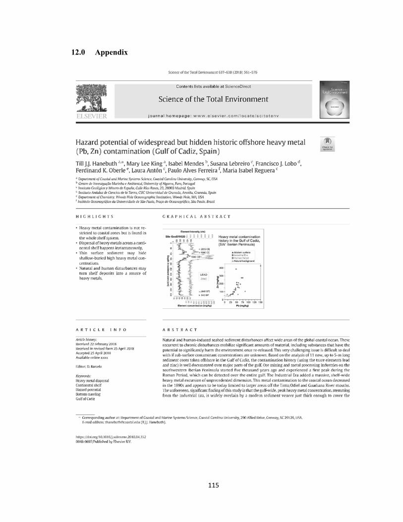
115  

12.0 Appendix