development of a laboratory apparatus to study the thermal

Development of a Laboratory Apparatus to Study the Thermal Degradation

Behavior of Commercial Jet Engine Oils

by

Amanda Jean Neer

A thesis submitted to the Graduate Faculty of

Auburn University

in partial fulfillment of the

requirements for the Degree of

Master of Science

Auburn, Alabama

May 7, 2012

Keywords: jet engine oils, thermal degradation,

fume event, air contamination

Copyright 2012 by Amanda Jean Neer

Approved by

Ruel A. Overfelt, Chair, Professor of Materials Engineering

Jeff Fergus, Professor of Materials Engineering

Bart Prorok, Associate Professor of Materials Engineering

ii

Abstract

Air quality on airplanes is a key priority of the Federal Aviation Association (FAA). It is

suspected that, although rare, oil leaks in the engine can potentially allow contaminants into the

air supply that is provided to the passengers in the cabin. Reliable and validated commercial

sensors would enable the air quality on the airplane to be monitored. Before sensors can be

utilized on airplanes a better understanding of the degradation behavior of jet engine oils is

needed. Although a few previous studies have reported on the reaction products produced during

thermal degradation of oil, the experimental set-ups used exhibited limited flexibility. Current

technology, such as thermogravimetric analysis (TGA), can provide the precise data and

information needed for understanding the thermal degradation behavior of jet engine oil, but

such laboratory instruments are expensive, can only evaluate small sample sizes, and constrain

the possible experimental protocols. The laboratory apparatus described in this thesis performs

the same functions as a TGA but it is reasonably inexpensive, accommodates samples up to 2 g,

and provides considerable flexibility in designing experimental protocols. The thermal

degradation system consists of a microbalance, a cylindrical furnace, and a crucible to hold the

sample. The system can be easily interfaced with other laboratory equipment such as custom

sensor chambers or a Fourier Transform Infrared Spectrometer (FTIR). The modes of heat

transfer of the thermal degradation system are characterized in this paper. Additionally,

preliminary results of the thermal degradation behavior of Mobil Jet Oil II are reported.

iii

Acknowledgments

I would like to express gratitude to Dr. Ruel A. Overfelt for his patience, compassion,

and guidance throughout this learning process. Under his tutelage, I have learned much about the

essential qualities of a good engineer. These lessons will leave a lasting impression on my career

path.

Many thanks are due to my committee members: Dr. Fergus and Dr. Prorok for their

support and for providing invaluable insight.

I also would like to express much appreciation to LC Mathison for all of his technical

support and expertise. It was through his skills that this project was made possible.

I would also like to acknowledge my fellow group members: John Andress, Lance

Haney, Shawn Yang, Naved Siddiqui, Wil Kilpatrick, and Briana McCall for their support,

insight, and friendship.

Last, but certainly not least, I would like to recognize the tremendous amount of support,

understanding, and encouragement that I have received from my family and friends. Through

them I have grown into the person I am today.

This project was funded by the U.S. Federal Aviation Administration (FAA) Office of

Aerospace Medicine through the National Air Transportation Center of Excellence for Research

in the Intermodal Transport Environment (RITE), Cooperative Agreement 07-C-RITE-AU.

Although the FAA has sponsored this project, it neither endorses nor rejects the findings of this

Research.

iv

Table of Contents

Abstract ........................................................................................................................................ ii

Acknowledgments ....................................................................................................................... iii

List of Tables .............................................................................................................................. vi

List of Figures ........................................................................................................................... viii

List of Symbols ............................................................................................................................ x

1 Introduction ............................................................................................................................... 1

2 Literature Review ...................................................................................................................... 6

2.1 Experimental Techniques Used to Thermally Degrade Jet Engine Oil ..................... 7

2.2 Thermal Degradation Behavior of Jet Engine Oil ..................................................... 9

2.3 Limitations of Previous Research ............................................................................ 12

3 Experimental Procedures and Analytical Techniques ............................................................ 14

3.1 Thermal Degradation System .................................................................................. 14

3.2 Experimental Protocol to Evaluate Heat Transfer Mechanisms .............................. 18

3.2.1 Experimental Arrangement to Evaluate Temperature Gradients

in Crucibles ............................................................................................... 22

3.2.2 Analysis of Convective Heat Transfer ....................................................... 23

3.2.3 Analysis of Radiative Heat Transfer ......................................................... 25

3.3 Experimental Arrangement to Evaluate Mass Measurements of System ................ 27

3.4 Experimental Arrangement to Thermally Degrade Jet Engine Oil .......................... 27

v

4 Results and Discussion ……………………………………………………………………... 30

4.1 Heat Transfer Analysis ............................................................................................ 30

4.1.1 Analysis of Temperature Measurements .................................................. 30

4.1.2 Convection ................................................................................................ 34

4.1.3 Radiation .................................................................................................. 39

4.1.4 Temperature Gradients in Crucibles ......................................................... 41

4.2 Mass Change Measurements .................................................................................... 42

4.3 Preliminary Results of Mobil Jet Oil II..................................................................... 45

4.3.1 Mass Change and Temperature Measurements ........................................... 45

4.3.2 Overall Appearance and Color Change ....................................................... 46

4.3.3 Preliminary Sensor Results .......................................................................... 47

5 Conclusions ……………………………………………………………………………….... . 49

References ................................................................................................................................. 50

vi

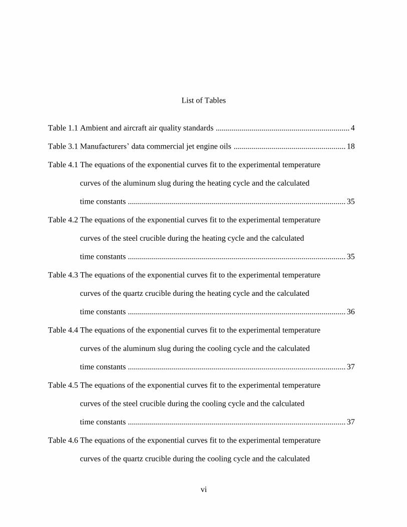
List of Tables

Table 1.1 Ambient and aircraft air quality standards ................................................................... 4

Table 3.1 Manufacturers’ data commercial jet engine oils ........................................................ 18

Table 4.1 The equations of the exponential curves fit to the experimental temperature

curves of the aluminum slug during the heating cycle and the calculated

time constants ............................................................................................................. 35


curves of the steel crucible during the heating cycle and the calculated

time constants ............................................................................................................. 35


curves of the quartz crucible during the heating cycle and the calculated

time constants ............................................................................................................. 36


curves of the aluminum slug during the cooling cycle and the calculated

time constants ............................................................................................................. 37


curves of the steel crucible during the cooling cycle and the calculated

time constants ............................................................................................................. 37


curves of the quartz crucible during the cooling cycle and the calculated

vii

time constants ............................................................................................................. 37

Table 4.7 Summary of the time constants calculated from the exponential

curve fits and their corresponding heat transfer coefficients for the

heating cycle .............................................................................................................. 39

Table 4.8 Summary of the time constants calculated from the exponential

curve fits and their corresponding heat transfer coefficients for the

cooling cycle ............................................................................................................. 39

Table 4.9 Power lost due to convection at each of the steady state temperatures ..................... 41

Table 4.10 Steady state temperatures for the center and OD of the steel crucible

with the overall percent difference ............................................................................ 41

Table 4.11 Steady state temperatures for the center and OD of the quartz crucible

with the overall percent difference ............................................................................ 42

viii

List of Figures

Figure 1.1 Diagram of the bleed air system of a Boeing 767 ....................................................... 2

Figure 2.1 Schematic of TGA arrangement ................................................................................. 8

Figure 2.2 TGA and DTA plot of pentaerythritol derivative in air ........................................... 11

Figure 3.1 Thermal degradation system ..................................................................................... 15

Figure 3.2 Steel crucible, Al slug, quartz crucible used in the experiment ...…………………. 18

Figure 3.3 Cross-sectional view of the position of Al slug in furnace ....................................... 19

Figure 3.4 Cross-sectional view of the position of quartz crucible in furnace .......................... 20

Figure 3.5 Cross-sectional view of the position of steel crucible in furnace .............................. 21

Figure 3.6 Holder to hold thermocouples in place ...................................................................... 22

Figure 3.7 Schematic of experimental set-up for oil degradation ............................................... 29

Figure 4.1 Temperature profiles for aluminum slug for various furnace set points .................. 30

Figure 4.2 Temperature profiles for steel crucible for various furnace set points ..................... 31

Figure 4.3 Temperature profiles for quartz crucible for various furnace set points ................... 31

Figure 4.4 Calibration curve for crucibles ................................................................................. 33

Figure 4.5 Comparison of the predicted temperature curve due to radiation with the

experimentally determined curve ............................................................................. 40

Figure 4.6 Mass change of Aeroshell 560 Turbine Oil at a furnace set point of 375°C ............ 44

Figure 4.7 Mass change of Aeroshell 560 Turbine Oil as a function of furnace

temperature for a set point of 375°C ........................................................................ 44

ix

Figure 4.8 Mass change rate of Aeroshell 560 Turbine Oil at a furnace set point of 375°C ..... 45

Figure 4.9 Plot of the oil mass (dashes) and temperature as functions of time ......................... 46

Figure 4.10 a) Mobil Jet Oil II before thermal degradation, b) after thermal degradation ........ 46

Figure 4.11 a) Bell jar before degradation experiment, b) smoke-filled bell jar

during degradation experiment ................................................................................ 47

Figure 4.12 Plot of the change in CO concentration as a function of time as measured by the

TGS5042 sensor (circles) and the FTIR (diamonds) and mass change (dashes)

as a function of time ................................................................................................. 48

Figure 4.13 Plot of the change in CO2 concentration as a function of time as measured by the

EE80 (circles) and the FTIR (diamonds) and the mass change (dashes) as a

function of time ........................................................................................................ 48

x

List of Symbols

A surface area

a constant

APU auxiliary power unit

CO carbon monoxide

CO2 carbon dioxide

cp specific heat capacity

ET total thermal energy

F12 view factor

FAA Federal Aviation Administration

FTIR Fourier Transform Infrared Spectrometer

GC/MS gas chromatography/mass spectrometry

h heat transfer coefficient

m mass

NDIR non-dispersive infrared

NOx nitrous oxides

O2 oxygen

O3 ozone

OD outer diameter

Qconv heat transferred by convection

xi

Qs→surr heat transferred by radiation from the sample to the surroundings

T temperature of sample

TCP tricresyl phosphate

TGA thermogravimetric analysis

Ts temperature of sample

Ti initial temperature

Tsurr temperature of surroundings

t time

VOC volatile organic compound

ε emissivity

σ Stefan-Boltzman constant

τ thermal time constant

1

1. Introduction

The average person spent approximately 34 hours sitting in traffic according to a report by

the Texas Transportation Institute in 2009. Sitting in traffic costs the economy about $115 billion

a year and that figure is expected to grow [1]. In addition to traffic, road travelers also have to

worry about unexpected construction delays. It is easy to see why many people might opt to take

an airplane for long distance trips. Many airlines offer to let the passenger sit back and relax

while flight attendants take care of their needs as they are jetted to their destination. As

passengers dream of sunny beaches or meeting with loved ones and flight crew members work

diligently to ensure the passengers have a restful journey, the last thing on anyone’s mind should

be the quality of the air in the cabin. However, the airlines have recently been receiving some

bad press about poor cabin air quality that is suspected to have made passengers and crew

members sick [2-6].

Poor air quality could potentially be caused by people on the airplane giving off metabolic

odors and exhaling carbon dioxide, or possibly air contaminants from fluid leaks in the air supply

system [7]. Potential sources of air contaminants include a variety of aircraft working fluids,

such as de-icing fluid, hydraulic fluid, jet fuel or jet engine lubricants. These fluids can enter the

airliner cabin through the bleed air supply from the engines during flight or from the auxiliary

power unit (APU) during ground operations. This situation will be referred to as a “fume event”

throughout the rest of this thesis.

2

Most commercial aircraft are powered by gas turbine engines with the turbofan engine being

the most common type, shown on the far left of Figure 1.1. A modern turbofan jet utilizes the

combusted and rapidly expanding pressurized gas to spin a turbine producing the mechanical

power to drive the ducted by-pass fan producing propulsion forces [8-11]. The driveshaft

assembly is lubricated with aircraft-grade grease or oil to prevent damage to the engine at the

extreme operational temperatures and pressures. About 1/5 of the air that enters the engine goes

through the core where some of it is extracted by bleed ports during the compression stage

(denoted by H and I in Figure 1.1). The bulk of the air goes through the by-pass where most of

the thrust is produced [7]. In the compression stage, the air can reach temperatures as high as

650°C. The air extracted from the bleed ports supplies hot compressed air to the bleed air system.

In the bleed air system, shown schematically in Figure 1.1, the air goes through a series of

valves and a heat exchanger to bring the air to the proper temperature and pressure to power all

pneumatic services on an airplane [7, 12]. Some of these services include the air-conditioning

packs and cabin pressurization. In a typical bleed air system, the temperatures can range from

170˚C during ground operations to 350˚C during takeoff. (The aircraft is powered by an APU

Figure 1.1: Diagram of the Bleed System of a Boeing 767 [7].

3

during ground operations.) During cruise, the temperature of the bleed air system is

approximately 250˚C [13]. The pressure of the bleed air from the engine can range from 1,170

kPa during takeoff to 340 kPa during cruise to 200 kPa during the initial descent[13].

Since the 1960s, jet engine oils and greases have been made of synthetic lubricants from the

neopentyl polyol ester group. These esters were chosen because of their superior performance

compared to petroleum-based lubricants, although additional additives are typically utilized for

further enhancement of their lubricating properties. Van Netten [2, 3] and Winder et al [14] have

found that these synthetic lubricants, when subjected to the high temperatures found in a jet

engine, can release toxic gases. Some of these gases include carbon monoxide (CO), carbon

dioxide (CO2), and/or tricresyl phosphate (TCP) (a known neurotoxin, used as an anti-wear

additive in engine oil). These contaminants can cause discomfort and in extreme cases threaten

the health and safety of those exposed. Several cases have been reported by flight crew members

of smoke, haze, and fumes entering the aircraft cabin and causing symptoms such as headaches

and dizziness. In some cases, members of the flight crew were taken to the hospital for further

treatment. Some of these events were linked to de-icing fumes and hydraulic fluid leaks in the

engine [2].

The Federal Aviation Administration (FAA) has established regulations for how much

carbon monoxide, carbon dioxide, and ozone (O3) is safe in an aircraft cabin environment. The

FAA has yet to pass any regulations regarding particulates, nitrogen oxides (NOx), or volatile

organic compounds (VOC), which can also be present in fume events involving lubricants and

hydraulic fluids. Table 1.1 lists the air quality standards currently in place for aircraft [15].

Though there are standards to regulate what is safe for an aircraft, there are no regulations for

actually monitoring the amount of pollutants on the aircraft.

4

Symptoms such as headaches, dizziness, and nausea will begin to manifest in passengers and

the flight crew once CO concentrations are in the range of 70 to 220 ppm. Concentrations of 220

to 520 ppm will cause those on board to become incapacitated. Chances for survival at

concentrations above 520 ppm are greatly lessened [16, 17]. A study by the National Air

Pollution Control Administration (1970) found that exposure to 50 ppm of CO for 90 minutes

will impair time-interval discrimination and visual function [18]. These findings and recent fume

events on airplanes have placed pressure on the FAA to pass regulations that require monitoring

the air quality on airplanes. In order for the FAA to make informed decisions when passing such

regulations, an understanding of how the various aircraft working fluids degrade at elevated

temperatures is necessary.

Over the past decade, several researchers have studied the thermal degradation behavior of

various brands of lubricating oils as well as other types of aircraft working fluids.

Thermogravimetric analysis (TGA) is a method used commonly to understand the thermal and

Table 1.1: Ambient and aircraft air quality standards [15].

5

physical changes the oils experience when they degrade at high temperatures [2, 19-23]. TGA

involves using a microbalance and a furnace to measure mass changes of a sample as it is being

heated at a constant rate. With TGA it is possible to control the atmosphere around the sample

during the heating process and the technique is very sensitive to mass loss. However, there are

also disadvantages to using TGA to analyze the thermal properties of a sample. TGA can only

analyze sample sizes up to 20 mg, and there is no contact between the thermocouple and the

sample [24, 25]. Sample sizes this small may not be representative of the bulk oil properties.

More importantly, larger sample sizes would enable various droplet surface area to volume ratios

to be investigated. Also, it is useful to be able to correlate mass changes of the oil to specific

temperatures of the oil itself. A laboratory system is needed that can address these concerns as

well as perform the functions of the TGA.

In this study, a laboratory apparatus has been developed to evaluate the thermal degradation

behavior of commercial jet engine oils at various temperatures. This apparatus is capable of

characterizing the temperature as well as the mass of the oil simultaneously with a fair amount of

accuracy. Not only was the system inexpensive to build compared to the price of purchasing a

new TGA, but it also made it easier to control various operational parameters of the system, i.e.

weighing functions, thermocouple placement, etc. The balance makes it possible to analyze very

small sample sizes on the order of thousandths of a gram up to 2 grams. In addition to having a

control thermocouple in the furnace, another thermocouple is placed in the sample. The heat

transfer mechanisms of the apparatus have been characterized and a model has been developed.

The goal of this research is to develop and characterize an apparatus that can be exploited in

future research to further understand how jet engine oils degrade. This information will help

guide the future work to determine the best method to detect fume events on airplanes.

6

2. Literature Review

It is essential to have an understanding of the chemical degradation mechanisms of jet

engine oils at elevated temperatures in order to make informed decisions on any sensors that

could be put on airplanes to detect fume events. Information such as when smoke begins to

appear and at what temperature it first appears is important, because that can potentially indicate

the formation of CO detectable by commercial sensors. A few different methods have been

utilized by previous researchers. It seems that some of these methods were not very reliable and

that others could benefit from wider experimental capabilities. The studies done in the past have

merely heated the oil and noted smoke formation and oil color change while measuring the

evolved gases. This study describes a laboratory apparatus that can do all the things done by

previous researchers as well as measure the mass change and record direct measurements of the

oil temperature during degradation.

This literature review is divided into three sections. The first section is an overview of

methods that have been used by other researchers to evaluate the thermal degradation behavior of

jet engine oils, namely thermogravimetric analysis (TGA). The second section discusses the

findings of other researchers in the field of thermal degradation of jet engine oils. The third

section summarizes the limitations of the previous techniques used and discusses how this

research addressed these limitations.

2.1 Experimental Techniques Used to Thermally Degrade Jet Engine Oil

Many techniques have been utilized by various researchers to analyze the thermal

degradation behavior of jet engine oils. They vary from complex thermogravimetric analysis

7

(TGA) systems connected to Fourier Transform Infrared (FTIR) spectrometers or gas

chromatography/mass spectrometry (GC/MS) to simpler systems consisting only of a heating

element and a crucible. In this section, TGA systems will be discussed in detail.

TGA is a popular technique because it requires little set up and working instruments can

be purchased from reputable manufacturers. TGA measures the weight change of a sample as a

function of temperature/time. The mass change rate as a function of time can be used to interpret

the reaction kinetics samples experience and quantify any evolved and/or absorbed gases [24-

26]. For example, TGA can be used to evaluate loss of water, loss of solvent, decarboxylation,

pyrolysis, oxidation, etc.

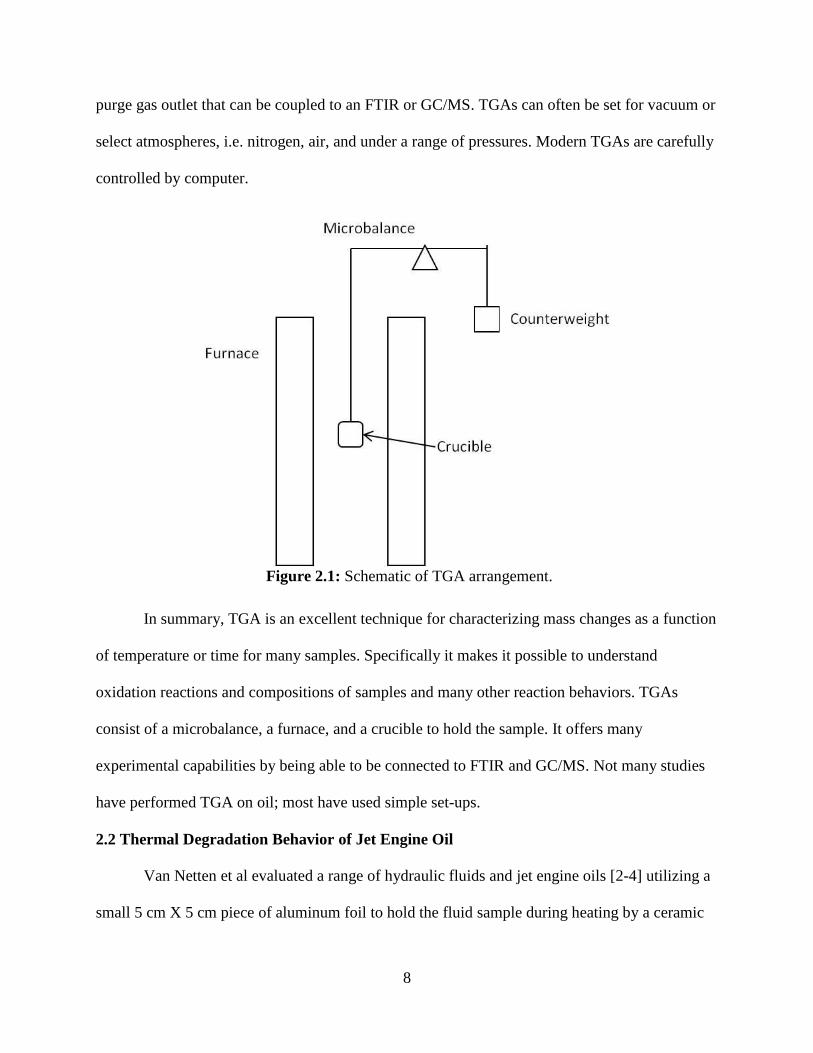
TGAs come in a variety of models that can be customized by the user. The set-up

modules may vary slightly, but the basic operation remains the same. This section describes a

typical set-up that is common to most TGAs and is shown schematically in Figure 2.1. TGAs

consist of a microbalance, a furnace, and a crucible to hold the sample. Quartz-crystal

microbalances in a TGA typically have a maximum sample size of 50 mg due to the dimensional

requirements for the crucibles and the furnace. The microbalance is electronically compensated

to account for movement of the crucible as the sample begins to gain or lose weight and is

extremely sensitive to mass loss. The furnace is raised and lowered around the stationary

crucible. The typical maximum operating range is from room temperature to 1000˚C and typical

heating rates range from 10°C/min to 20°C/min. The crucible is typically porcelain or platinum

because these materials are very stable at high temperatures. The crucible normally sits atop the

microbalance and the furnace is lowered into position, though in some models the crucible may

be attached to the microbalance from below. The sample temperature is measured by a

thermocouple at the sample crucible but not in the sample itself. Some TGAs are equipped with a

8

purge gas outlet that can be coupled to an FTIR or GC/MS. TGAs can often be set for vacuum or

select atmospheres, i.e. nitrogen, air, and under a range of pressures. Modern TGAs are carefully

controlled by computer.

In summary, TGA is an excellent technique for characterizing mass changes as a function

of temperature or time for many samples. Specifically it makes it possible to understand

oxidation reactions and compositions of samples and many other reaction behaviors. TGAs

consist of a microbalance, a furnace, and a crucible to hold the sample. It offers many

experimental capabilities by being able to be connected to FTIR and GC/MS. Not many studies

have performed TGA on oil; most have used simple set-ups.

2.2 Thermal Degradation Behavior of Jet Engine Oil

Van Netten et al evaluated a range of hydraulic fluids and jet engine oils [2-4] utilizing a

small 5 cm X 5 cm piece of aluminum foil to hold the fluid sample during heating by a ceramic

Figure 2.1: Schematic of TGA arrangement.

9

hot plate. A thermocouple was used to monitor the temperature of the hot plate. Gases were

evolved in a 250 L stainless steel chamber equipped with a multigas monitor TMX-412

(Industrial Scientific Corporation, Oakdale, PA) to measure NO2, oxygen (O2), and CO.

Additionally, a YES-204A monitor (Young Environmental Systems, Richmond, B.C., Canada)

was also in the chamber to measure temperature, relative humidity, and CO2 concentration [4].

The hot plate with the aluminum foil holder containing the test fluid was first placed into the

chamber and then heated to 525°C at a rate of 10°C/min. Samples were then isothermally held

for 1 minute at 525°C before being allowed to cool to room temperature. Air sensors began

recording the ambient air before the oil was inserted into the test chamber. Also, air samples

were retrieved from the chamber for later analysis by GC/MS.

Van Netten et al [2] noted that the Mobil 254 jet engine oil was initially dark blue in

color at room temperature. When the hot plate reached approximately 275°C white smoke began

to form and the oil turned a dark brown-orange color. At 400°C, it was noted that charring of the

oil began to occur and the white smoke continued to form. At 500°C, some charred material

remained on the aluminum foil sheet. Approximately 102.5 ppm CO and 460 ppm CO2 were

detected at 525°C [2]. Air sample results from GC/MS analysis indicated the presence of TCP

isomers as well as volatile derivatives of pentane, hexane, and octane during degradation of

Mobil 254 jet engine oil.

Castrol 5000 was orange in color at room temperature and began producing white smoke

at approximately 285°C. Darkening of the oil began at 310°C and charring was observed at

350°C. At the end of the experiment only charred brown material remained. The CO2 sensor

measured roughly 510 ppm CO2. The CO sensor detected approximately 140 ppm CO from

Castrol 5000 [4].

10

Van Netten et al [2] noted that Exxon 2380 was light orange in color at room

temperature. At about 275°C, the oil began producing white smoke. Darkening of Exxon 2380

began at 300°C and charring was observed at 310°C. At the end of the experiment only charred

brown material remained. The CO2 sensor measured roughly 510 ppm CO2 and the CO sensor

measured about 120 ppm CO [4]. GC/MS analysis of the gases produced by degrading Castrol

5000 and Exxon 2380 indicated that the components of the evolved gases were very similar to

one another. NO2 was not detected during degradation of any of the oil samples.

Crane et al [27] also evaluated Exxon 2380. These authors utilized a custom-built

combustion chamber to analyze evolved gas samples. The Crane et al [27] chamber had a much

smaller total volume of approximately 12.6 L. Three milliliters of sample was placed in a semi-

cylindrical quartz combustion boat, 7.5 cm long by 4 cm wide. The boat was placed in a

horizontal quartz tube with a 5 cm diameter and was 33 cm long. Two semi-cylindrical heating

elements encapsulated the quartz tube and the temperature was controlled by a thermocouple

placed in one of the heating elements. The sample was continuously heated from room

temperature until only charred material remained. Exxon 2380 began producing a measurable

amount of CO around 306°C at roughly the same time the authors noticed an increase in visible

smoke production. At 344°C, CO concentration was measured at 5,000 ppm CO and at 350°C

only charred material remained. The solid char continued to produce CO up to 530°C. When the

oil was exposed to 600°C, the authors reported a much higher CO level of 17,000 ppm CO.

Bartl et al [23] evaluated pentaerythritol derivatives (the base component of jet engine

oils) using TGA. These researchers heated 10 mg of pentaerythritol from room temperature to

1000°C at 10°C/min in air. Figure 2.2 shows TGA and DTA (differential thermal analysis) data

of a pentaerythritol derivative in air. The weight change data shows that the sample began to lose

11

mass at approximately 275°C, which is roughly the temperature Van Netten et al [2] began

seeing the oils generate smoke. Also DTA data indicates sample heating due to exothermic

reactions (i.e., burning) in the oil as the oil degrades. The first peak at approximately 350°C

corresponds to an oxidation reaction in which volatile reaction products are produced. The

second peak at about 570°C is due to the oxidation of the carbonaceous fraction to CO and CO2.

This can be roughly correlated to the CO and CO2 evolution reported by Van Netten at 525°C.

Van Netten et al [2, 4] and Crane et al [27] noted the temperatures at which the oils began

to smoke. Van Netten reported that Mobil 254 and Exxon 2380 began producing smoke at about

275°C. Castrol 5000 began producing smoke at 285°C. Crane reported that Exxon 2380 began

producing smoke at 306°C. Differences in the temperature that Exxon 2380 began smoking may

be attributed to the different arrangements used. Van Netten et al used a hot plate and so the oil

was only being heated from the bottom. The thermocouple that was used to record the

Figure 2.2: TGA and DTA plot of pentaerythritol derivative in air [23].

12

temperature was simply laid on top of the hot plate also and it is possible that some heat loss due

to the surrounding air may have occurred resulting in a lower temperature reading. Crane et al

placed the oil in a ceramic boat in a quartz tube that was surrounded by a heating element. This

method provided the sample with better uniform heating and additionally the thermocouple was

embedded inside the furnace reducing the amount of heat loss to the surroundings. The slight

differences between the oils evaluated by Van Netten can possibly be attributed to variations in

the components of the oils.

2.3 Limitations of Previous Research

One limitation of much of the previous research involves the actual temperature of the oil

when it is being degraded. Having a thermocouple directly in the oil would enable more reliable

characterization of the oil temperature in the event that it lags the heating element during heat-up

or leads the heating element during exothermic reactions. Such data are important to precisely

understand the thermal degradation reaction kinetics. Reliable temperature measurements would

also make it possible to calculate convective heat transfer coefficients. This would also lead to a

better understanding of how the oil is degrading.

In addition, all of the previous studies evaluated relatively small sample sizes. Crane et al

used about 3 g of oil. Larger sample sizes would enable various oil droplet surface area to

volume ratios to be used and allow oil degradation to be analyzed using standard combustion

techniques.

In summary, none of the studies reviewed directly measured the temperature of the oil as

it was heating. This is important for understanding the degradation behavior of the oil. The

studies in this review evaluated relatively small sample sizes. Larger sample sizes may provide a

better idea of bulk oil behavior during degradation. Mass change was not taken into account by

13

Van Netten and Crane. Recording mass changes during degradation should enhance our

understanding of the degradation behavior of the oil.

14

3. Experimental Procedures and Analytical Techniques

3.1 Thermal Degradation System

A laboratory apparatus has been developed to thermally degrade aircraft working fluids.

The thermal degradation system was used to degrade jet engine oils at various elevated

temperatures. This system, shown in Figure 3.1, incorporated a microbalance from which the

fluid samples were suspended into a cylindrical ceramic fiber furnace. This arrangement is

similar to a TGA except that larger samples and unique experimental protocols can be

investigated. The microbalance – furnace assembly was housed within a 50 L bell jar to contain

any evolved gases that were produced during experiments. The entire thermal degradation

system was further enclosed by a custom built fume hood to contain any possible leaks in the

system for additional safety.

There were two plastic tubes of 12 mm inner diameter and 61 cm length on either side of

the furnace that drew room temperature air from the room into the top of the bell jar where the

microbalance was housed. The airflow direction is indicated by the blue dashed arrows in Figure

3.1. The air flow from the plastic tubes was directed around the microbalance and then through a

hole beneath the microbalance, and down the length of the furnace passing over the suspended

crucible assembly where any evolved gases or smoke could be entrained within the air stream.

The furnace was hollow in the center and open on both ends allowing air to flow all the way

through to an opening in the base plate that is connected to a six-way cross. A six-way cross at

the bottom allowed the air stream to be coupled to other laboratory analysis equipment, i.e.

15

unique sensor chambers, a Fourier Transform Infrared spectrometer (FTIR), etc. The air stream

was powered by an 11,600 sccm vacuum pump during and after the experiments.

1) Microbalance

The thermal degradation system utilized a Scientech SM124D microbalance (Boulder,

CO) to measure changes in mass of the experimental working fluid during thermal exposures.

The microbalance had a dual range mode: one with a maximum capacity range of 40 g and the

other with a maximum capacity of 120 g. For all the experiments in this study, the 120 g range

was used. The microbalance enabled measurements of mass within ±0.6 mg over the

experimental mass range. The microbalance had a “below balance” or a “hang down” weighing

mechanism that enabled the crucible suspension assembly to be inserted into the furnace while

characterizing the mass. Balance calibration was checked and verified prior to any evolved gas

experiments using calibration weights of known mass. The balance calibration was verified

Figure 3.1: Thermal Degradation System.

Furnace

16

every day that the balance was used to ensure minimal error in the mass measurements. On

average, the measured values from the balance tended to be slightly lower than the reported

values for the calibration weights, but agreement was typically within 0.027% of the reported

value. The microbalance was controlled externally by a computer. All of the data recorded from

the microbalance were analyzed with Microsoft Excel 2007®.

The microbalance was located approximately 8 cm above the furnace. A 2.5 cm layer of

ceramic fiber board was used to insulate the balance from the furnace underneath. The fiber

board was wrapped in aluminum foil and then sandwiched between two layers of aluminum, 12

mm thick on top and 1.5 mm thick on bottom. The aluminum and fiber board were supported by

four aluminum legs approximately 2.5 cm in diameter. The crucible was attached to the

microbalance from below and hung through the same hole that air was drawn through as

discussed earlier. There were alignment holes on the bottom of the legs that matched pegs in the

base plate to ensure repeatable placement. Finally, a 1.5 mm thick rubber gasket formed a

compression seal between the 12 mm thick microbalance support plate and the inside of the bell

jar to ensure that air flow was always from the microbalance area through the crucible hang

down hole, through the furnace and out of the system to protect the microbalance from possible

contamination during thermal degradation experiments.

2) Furnace

A cylindrical ceramic fiber furnace (Watlow, Chicago, IL) was used to heat the working

fluid samples to the desired temperatures. The heating elements were composed of a high

temperature iron-chrome-aluminum alloy and were insulated by an alumina-silica compound.

The operating parameters of the furnace, i.e. temperature set point and heating rate, were

adjusted by a furnace controller (Watlow, Chicago, IL). The furnace had an outer diameter of 10

17

cm, an inner diameter of 5 cm and was approximately 15 cm in height. The maximum operating

temperature of the furnace was 2200˚C. A 2 mm diameter through hole was fabricated in the

furnace side about 7 cm from the top for location of a furnace control thermocouple.

Type K thermocouples (Omega Engineering Inc., Stanford, CT), insulated with ceramic

tubes and woven ceramic fiber, were used for all temperature measurements. The reliability of

the thermocouples was checked by measuring the boiling point of water. The thermocouple

measurements agreed within 1% of the boiling point of water. A thermocouple was placed in the

experimental fluid sample for all thermal degradation measurements and was also attached

securely to the bottom of the microbalance support structure to eliminate inadvertent contact

between the thermocouple and the hang down assembly and to minimize movement of the

thermocouple within the fluid sample. All data recorded from the thermocouples were analyzed

using Microsoft Excel 2007®.

3) Working Fluid Samples: Jet Engine Oils

Two commercial jet engine oils were selected for this study: Aeroshell 560 (Shell

Aviation) and Mobil Jet Oil II (ExxonMobil) because they are the most commonly used in the

airline industry. The properties for each of the oils are given in Table 3.1. The base component of

these jet engine oils is 95% pentaerythritol. The oils also contain 2 – 4% antioxidants, such as N-

phenyl-2-naphthylamine and 1 – 3% antiwear additives, such as tricresyl phosphate. In addition,

corrosion inhibitors, rust inhibitors, and anti-foaming agents are also typically added to enhance

the performance of the oils [14, 28, 29]. It was assumed that both of the oils had the same heat

capacity because they have similar base components. The oils were stored in air tight containers

at room temperature.

18

3.2 Experimental protocol to evaluate heat transfer mechanisms

Three materials were used to investigate the heat

transfer mechanisms occurring in the thermal degradation

system. Initially, a 6061 aluminum slug, shown in Figure

3.2, was used to develop heat transfer models because its

thermal properties have been well-documented [30-32]. The

models developed were then applied to fused quartz and

stainless steel crucibles, also shown in Figure 3.2. These crucibles were planned for usage with

the oil samples. The quartz crucible had a volume of 20 milliliters while the steel crucible had a

volume of 50 milliliters.

Each of the crucibles was attached by a copper wire through two holes on either side and

then suspended in the center of the furnace as discussed in section 3.1. The aluminum slug had a

through-hole in the center to allow for the placement of a thermocouple. For the experiments

with the crucibles, the thermocouple was placed in contact with the crucible bottom and

positioned as close to the center of the crucible bottom as possible. Figures 3.3, 3.4, and 3.5

show cross-sectional views of the positions of the aluminum slug, the quartz crucible, and the

steel crucible in the furnace during the heating portion of the experiments.

Aeroshell 560 Mobil Jet Oil II

Color amber amber

Density [g/cm^3] 0.996 1.00

Flash Point [˚C] 260 270

Auto ignition Temp [˚C] 320 404

Heat Capacity @constant P [J/Kg K] 2130 2130

Table 3.1: Manufacturers’ data on commercial jet engine oils [28,29].

Figure 3.2: Steel crucible, Al

slug, quartz crucible used in

the experiments.

19

Figure 3.3: Cross-sectional view of the position of Al slug in furnace.

20

Figure 3.4: Cross-sectional view of the position of quartz crucible in furnace.

21

Figure 3.5: Cross-sectional view of the position of steel crucible in furnace.

22

The experimental protocol for the heat transfer experiments was carried out with the following

steps:

1. The appropriate crucible or aluminum slug was attached to a copper wire and suspended

from the microbalance support assembly.

2. The furnace was preheated to the desired temperature.

3. The furnace was allowed to stabilize (approximately one hour).

4. The appropriate crucible or aluminum slug was placed in the furnace for one hour.

5. Temperature measurements were recorded at a rate of 1 Hz for both heating and cooling.

6. The system was allowed to cool to room temperature.

Furnace set point temperatures of 300, 350, 400, 450, and 500°C were used for these heat

transfer measurements. Each of the samples was evaluated at each of the set points and repeated

to ensure repeatability. These temperatures were chosen to represent the range of exposure

temperatures anticipated for the various working fluids of interest.

3.2.1 Experimental Arrangement to evaluate temperature gradients in crucibles

The temperatures in the center and of the outer diameter of the crucibles were measured

to examine the temperature gradients across crucibles

containing one milliliter of Aeroshell 560 Turbine oil. The

purpose of this experiment was to determine the sensitivity

of thermocouple location on the crucible temperature

measurements. The experimental protocol for

characterizing the crucible temperature gradients was

carried out with the following steps:

1. One milliliter of Aeroshell 560 Turbine Oil was

Figure 3.6: Holder to hold

thermocouples in place.

23

placed into the crucible.

2. As shown in Figure 3.6, a wire mesh was used to minimize thermocouple movement in

the crucible. Two thermocouples were placed into the crucible – one at the center using

the holder as a guide and a second thermocouple at the outer diameter of the crucible.

3. The crucible was suspended into position within the furnace.

4. The furnace was set to 375°C with a heating rate of 10°C/min.

5. Temperature measurements were collected at a rate of 1 Hz.

This experiment was repeated for the quartz crucible and each experiment was performed three

times for both crucibles.

3.2.2 Analysis of Convective Heat Transfer

There were three modes of heat transfer within the thermal degradation system:

conduction, convection, and radiation. Conduction occurs within materials subjected to

temperature gradients. Convective heat transfer occurs between solids and fluids at different

temperatures. Non-contact radiation heat exchange can occur when two bodies at different

temperatures are in line-of-sight of each other.

Newton’s Law of Cooling is often used to describe convective heat transfer:

ssurrconv TThAQ . (3.1)

Qconv is the convective heat transferred between the center of the sample and the fluid, h is the

convective heat transfer coefficient, A is the surface area of the sample being heated, Tsurr is the

temperature of the surroundings, and Ts is the temperature of the material. During the heating

cycle, Tsurr is the temperature of the furnace and during the cooling cycle it is the temperature of

the environment surrounding the sample. A requirement of Newton’s Law is that the convective

heat transfer coefficient remains constant, i.e. the heat flow per unit area is proportional to the

24

temperature difference between the sample and the surrounding fluid. The heat transfer

coefficient has thus been assumed to be constant in this analysis. The thermophysical properties

of the materials were also assumed to be constant.

The total thermal energy ET stored in a sample at a given temperature can be defined as

spT TmcE (3.2)

where m is the mass of the sample, cp is the specific heat capacity of the sample, and Ts is the

temperature of the sample. Differentiating the total thermal energy with respect to time yields

dt

dTmc

dt

dE sp

T (3.3)

which can be set equal to Equation (3.1) to obtain

ssurrs

p TThAdt

dTmc (3.4)

Rearranging Equation (3.4) so that it can easily be integrated over temperature and time

gives

s

i

T

T

t

pssurr

s dtmc

hA

TT

dT

0

(3.5)

where the left hand side is integrated from initial temperature, Ti, to final sample temperature, Ts;

and the right hand side is integrated from 0 to time, t. Ts is the dependent variable. Integration of

both sides yields

t

p

T

Tssurr tmc

hATT

s

i 0ln

(3.6)

Substituting in the integration limits gives

p

isurrssurrmc

hAtTTTT

lnln (3.7)

Solving for the final sample temperature yields

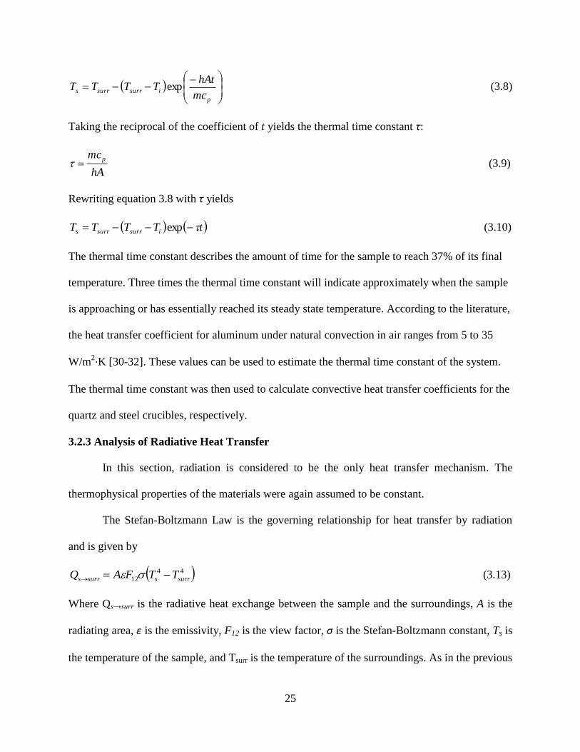
25

p

isurrsurrsmc

hAtTTTT exp (3.8)

Taking the reciprocal of the coefficient of t yields the thermal time constant τ:

hA

mcp (3.9)

Rewriting equation 3.8 with τ yields

tTTTT isurrsurrs exp (3.10)

The thermal time constant describes the amount of time for the sample to reach 37% of its final

temperature. Three times the thermal time constant will indicate approximately when the sample

is approaching or has essentially reached its steady state temperature. According to the literature,

the heat transfer coefficient for aluminum under natural convection in air ranges from 5 to 35

W/m2·K [30-32]. These values can be used to estimate the thermal time constant of the system.

The thermal time constant was then used to calculate convective heat transfer coefficients for the

quartz and steel crucibles, respectively.

3.2.3 Analysis of Radiative Heat Transfer

In this section, radiation is considered to be the only heat transfer mechanism. The

thermophysical properties of the materials were again assumed to be constant.

The Stefan-Boltzmann Law is the governing relationship for heat transfer by radiation

and is given by

44

12 surrssurrs TTFAQ (3.13)

Where Qs→surr is the radiative heat exchange between the sample and the surroundings, A is the

radiating area, ε is the emissivity, F12 is the view factor, σ is the Stefan-Boltzmann constant, Ts is

the temperature of the sample, and Tsurr is the temperature of the surroundings. As in the previous

26

section, Tsurr is the temperature of the surrounding environment. The crucible was assumed to be

in complete line-of-sight of its surroundings thus allowing one to assume a geometric view factor

of one. Equation (3.13) can be set equal to the right hand side of equation (3.3):

44

surrss

p TTAdt

dTmc (3.14)

If Ts is very large compared to Tsurr, then it can be assumed that 4

surrT is insignificant. To

integrate this equation over time and temperature, it is rearranged to yield

s

i

T

T

t

ps

s dtmc

A

T

dT

0

4

(3.15)

where the left hand side is integrated from initial sample temperature to final sample temperature

and the right hand side is integrated from zero to time, t. Equation (3.15) is integrated over time

and temperature and rearranged to yield

t

p

T

Ts

tmc

A

T

s

i

033

1

(3.16)

Substituting for the integration limits yields

pis mc

tA

TT

33 3

1

3

1 (3.17)

From the previous equation it is possible to obtain the final temperature of the sample

31

33

13

1

ip

s

Tmc

tAT

(3.18)

27

3.3 Experimental Arrangement to Evaluate Mass Measurements of System

The mass measurements of the microbalance were evaluated with one milliliter of

Aeroshell 560 Turbine Oil in the quartz crucible. The purpose of this experiment was to

determine the repeatability of the mass measurements with the microbalance. The experimental

protocol for the mass measurements was carried out with the following steps:

1. One milliliter (1 g) of Aeroshell 560 Turbine Oil was placed into the quartz crucible.



4. Mass measurements were collected at a rate of 1 Hz.

The experiment was repeated 5 times. The mass change rate was calculated by taking the

difference of the mass over the change in time.

3.4 Experimental Arrangement to Thermally Degrade Jet Engine Oil

The capabilities of the system as a whole were evaluated with one milliliter of Mobil Jet

Oil II. The experimental protocol to thermally degrade the Mobil Jet Oil II was carried out with

the following steps:

1. One milliliter (1 g) of Mobil Jet Oil II was placed into the quartz crucible.

2. The thermocouple was centered without touching the bottom of the crucible.


4. The bell jar was placed over the balance – furnace assembly.

5. The door of the fume hood was secured.


7. Temperature and mass measurements were each collected at a rate of 1 Hz.

8. Once the set point was reached, the oil sample was held isothermally for one hour.

28

Measurements from commercial CO and CO2 sensors were also obtained at 5 minute

intervals and FTIR scans were taken every 2 minutes. Figure 3.7 shows a schematic of the

experimental set-up. For this study, a TGS 5042 CO sensor made by Figaro (Arlington Heights,

IL) and an EE80-2CT2/TO4 CO2 sensor made by AirTest (Delta, BC) were used [33]. The TGS

5042 is an electrochemical sensor that utilizes amperometry to calculate the CO concentration by

means of a working electrode and a counter electrode. Specific anions dissolved in an electrolyte

oxidize the CO present at the working electrode generating a current proportional to the CO

concentration. The sensor has an automatic calibration procedure to compensate for the aging of

the infrared source and dust contamination. The EE80 utilizes non-dispersive infrared (NDIR)

technology. The sensor has two single wavelength infrared sources. The first infrared source

continuously monitors the sample chamber whereas the second infrared source is used as a

reference signal for calibration. The sensor calculates the amount of CO2 present based on the

absorbed energy of the infrared beam after it has traveled through the sensors sample chamber.

The FTIR was a Perkin-Elmer Spectrum GX Fourier Transform Infrared Spectrometer and is

described in detail by Haney et al [34]. The sensors were housed in a sensor chamber separate

from the bell jar. A line was run from the six-way cross below the base plate to the sensor

chamber and from the sensor chamber to the FTIR. A vacuum pump connected to the FTIR

pulled air through the whole system at a rate of 11,600 sccm into the building exhaust.

29

Figure 3.7: Schematic of experimental set-up for oil degradation.

30

4. Results and Discussion

4.1 Heat Transfer Analysis

4.1.1 Analysis of Temperature Measurements

The heating and cooling temperature profiles of an aluminum slug, a stainless steel

crucible, and a quartz crucible were recorded for a range of furnace temperatures: 300, 350, 400,

450, and 500°C. The sample temperature change was plotted as a function of time and the plots

are shown in Figures 4.1, 4.2, and 4.3, respectively.

Figure 4.1: Temperature profiles for aluminum slug at the indicated furnace set points.

31

Figure 4.2: Temperature profiles for steel crucible at the indicated furnace set points.

Figure 4.3: Temperature profiles for quartz crucible at the indicated furnace set points.

32

Even though all three samples were evaluated with the same furnace set points, each

sample reached different final steady state temperatures. The quartz crucible is the only sample

whose steady state temperature was at or slightly above the furnace temperature. Quartz absorbs

certain infrared wavelengths emitted by radiative heat. The wavelengths absorbed are between

2.6 and 2.9, and above 3.6 μm [35, 36]. If these wavelengths are present in the furnace when

heating the quartz crucible may be absorbing them, which could potentially cause the quartz

crucible to gain additional heat from the absorbed wavelengths. The average temperature

difference between the furnace set point and the steady state temperature of the aluminum slug

was 110 ± 8°C. The average temperature difference between the furnace set point and the steady

state temperature of the steel crucible was 50 ± 5°C. The steady state temperature of the

aluminum slug and the steel crucible never equals the furnace set point because of heat losses

due to convection and radiation. The aluminum slug and the steel crucible lose heat to the

surroundings at different rates due differences in their respective geometries. The aluminum slug,

as shown in Figure 3.2, was a rectangle with a hole in the center for the thermocouple. The

aluminum slug heats from the outside and conducts heat inward to the thermocouple location.

This process is slow and possibly contributes to the large difference between the steady state

temperature of the aluminum slug and the furnace set point. Additionally, the rate of temperature

increase of the aluminum slug is also affected causing it to take longer to reach its steady state

temperature. The steel crucible, as shown in Figure 3.2, is a hollow, thin-walled cylinder with

one end closed. The sides of the crucible heat up first because they are in the line-of-sight of the

heater. Then heat is transferred to the bottom of the crucible.

33

The calibration curve for the crucibles is shown in Figure 4.4 and the curve for the

aluminum slug is also shown for comparison. The steady state temperature of each of the

samples is plotted with the furnace set point. For either crucible, the equations obtained from the

linear curve fit can be used to predict the final temperature of the empty crucible, which can

provide an approximation for the final temperature of the oil in the crucible.

The calibration curve shows that the quartz crucible had the highest steady state

temperature; the steel crucible had the second highest steady state temperature, and the

aluminum slug had the lowest steady state temperature. The steady state temperatures of the steel

crucible and the aluminum slug are lower than the furnace set point due to heat losses to the

surroundings. The steel crucible and the aluminum slug also have reflective surfaces that reflect

heat away causing the thermocouple to measure lower temperatures. As mentioned previously,

Figure 4.4: Calibration curve for the crucibles.

34

the quartz crucible absorbs certain wavelengths of radiative heat, which may cause it to have a

higher temperature than its surroundings. In this case, the quartz crucible may potentially radiate

heat to the surrounding air and maintain a temperature at or slightly above the furnace set point.

Additionally, the quartz had the lowest uncertainty and the steel crucible had the largest

uncertainty in temperature measurements. According to these results, the quartz crucible is the

best candidate for oil thermal degradation experiments because of its low uncertainty.

4.1.2 Convection

Convection was initially considered to be the only heat transfer mechanism occurring in

the system. Convective heat transfer coefficients were estimated for the aluminum slug, the steel

crucible, and the quartz crucible. The equations of the exponential curve fits and the time

constants calculated from these equations for the aluminum slug, the steel crucible, and the

quartz crucible during the heating cycle are presented in Tables 4.1, 4.2, and 4.3, respectively.

According to Table 4.1, the time constants calculated from the exponential curve fits for the

aluminum slug during the heating cycle range from approximately 200 to 250 s. The

corresponding heat transfer coefficients for these time constants are 20 to 25 W/m2·K where the

lower heat transfer coefficient is associated with the higher time constant. The time constant

decreases as the furnace set point increases. A smaller time constant indicates that the sample is

responding faster to its environment. This is a possible indication of radiation contributing to

heat transfer between the aluminum slug and the surroundings.

According to Table 4.2, the time constants calculated from the exponential curve fits for

the steel crucible during the heating cycle range from approximately 60 to 90 s. The

corresponding heat transfer coefficients for these time constants are 20 to 30 W/m2·K. Even

though the aluminum slug and the steel crucible have similar heat transfer coefficients the time

35

constants are different because they are dependent on material properties, such as specific heat

capacity. Aluminum has a specific heat capacity of 896 J/kg·K and steel has a specific heat

capacity of 500 J/Kg·K. Specific heat capacity describes the amount of energy required to change

one unit of mass of a substance by one unit of temperature. The lower specific heat capacity a

substance has the less energy that is required to raise its temperature. In this case, the steel has a

lower specific heat capacity and thus requires less energy to raise its temperature, in turn

requiring less time to reach 37% of its final temperature. The mass and the surface area also

contribute to the time constant. A larger mass increases the time constant while larger surface

areas decrease the time constant.

Furnace Set

Point [°C] Equation R2

Time

Constant [s]

300 Ts = 149e-0.00404t

0.987 248

350 Ts = 186e-0.00414t

0.991 242

400 Ts = 211e-0.00444t

0.99 225

450 Ts = 305e-0.00509t

0.999 196

500 Ts = 266e-0.00490t

0.991 204

Table 4.1: The equations of the exponential curves fit to the

experimental temperature curves of the aluminum slug during the

heating cycle and the calculated time constants.

Furnace Set


Time

Constant [s]

300 Ts = 277e-0.0117t

0.988 85

350 Ts = 418e-0.0109t

0.984 92

400 Ts = 383e-0.0146t

0.987 68

450 Ts = 395e-0.0124t

0.971 81

500 Ts = 563e-0.0170t

0.988 59


experimental temperature curves of the steel crucible during the


36

According to Table 4.3, the time constants calculated from the exponential curve fits for

the quartz crucible during the heating cycle range from approximately 70 to 110 s. The

corresponding convective heat transfer coefficients for these time constants are 30 to 45 W/m2·K.

Also the convective heat transfer coefficient values calculated for quartz are a little higher than

those calculated for the aluminum slug and the steel crucible. This indicates that radiation is

likely contributing to heat transfer for the quartz. This is plausible considering that quartz is

nearly invisible to radiation as mentioned previously and so it is reasonable that radiation would

be more apparent in the quartz crucible calculations than the aluminum slug or the steel crucible.

The equations of the exponential curve fits and the time constants calculated from these

equations for the aluminum slug, the steel crucible, and the quartz crucible during the cooling

cycle are presented in Tables 4.4, 4.5, and 4.6, respectively. According to Table 4.4, the time

constants calculated from the exponential curve fits for the aluminum slug during the cooling

cycle range from approximately 330 to 500 s. The corresponding convective heat transfer

coefficients for these time constants are 10 to 15 W/m2·K.

Furnace Set


Time

Constant [s]

300 Ts = 296e-0.0100t

0.993 100

350 Ts = 387e-0.0129t

0.999 78

400 Ts = 299e-0.00891t

0.903 112

450 Ts = 484e-0.0147t

0.995 68

500 Ts = 385e-0.0121t

0.986 83


experimental temperature curves of the quartz crucible during the


37

According to Table 4.5, the time constant calculated from the exponential curve fits for

the steel crucible during the cooling cycle range from approximately 115 to 125 s. The

Furnace Set


Time

Constant [s]

300 Ts = 179e-0.00200t

0.932 500

350 Ts = 230e-0.00214t

0.904 467

400 Ts = 265e-0.00219t

0.911 457

450 Ts = 297e-0.00201t

0.961 498

500 Ts = 344e-0.00223t

0.927 448


experimental temperature curves of the aluminum slug during the

cooling cycle and the calculated time constants.

Furnace Set


Time

Constant [s]

300 Ts = 236e-0.00792t

0.995 126

350 Ts = 407e-0.00816t

0.978 123

400 Ts = 336e-0.00869t

0.995 115

450 Ts = 441e-0.00796t

0.995 126

500 Ts = 392e-0.00806t

0.993 124


experimental temperature curves of the steel crucible during the


Furnace Set


Time

Constant [s]

300 Ts = 276e-0.00620t

0.999 161

350 Ts = 319e-0.00643t

0.998 156

400 Ts = 347e-0.00638t

0.996 157

450 Ts = 380e-0.00636t

0.990 157

500 Ts = 425e-0.00706t

0.9957 142


experimental temperature curves of the quartz crucible during the


38

corresponding convective heat transfer coefficient for the time constants is 15 W/m2·K.

According to Table 4.6, the time constants calculated from the exponential curve fits for the

quartz crucible during the cooling cycle range from approximately 140 to 160 s. The

corresponding convective heat transfer coefficients for these time constants are 15 to 20 W/m2·K.

During the cooling cycle, the samples did not show much variation in the thermal time constants.

Quartz exhibited the largest calculated heat transfer coefficient. According to the previous

section, quartz loses very little if any heat to its surroundings during heating. The convective heat

transfer coefficient is proportional to the heat flux and the temperature difference between the

sample and its surroundings. The quartz crucible has a larger convective heat transfer coefficient

because it is not losing as much heat per unit area as the steel crucible or the aluminum slug. The

heat transfer coefficients are much larger on heating than the heat transfer coefficients calculated

on cooling, because during heating there are multiple heat transfer mechanisms occurring, i.e.

convection and radiation. On cooling, convection appears to be the dominant mode of heat

transfer.

The convective heat transfer coefficients and time constants calculated for the aluminum

slug, the steel crucible, and the quartz crucible at each of the furnace set points were consistent.

This allowed averages to be calculated for the values of the heat transfer coefficients and the

time constants at each of the furnace set points. The results of these calculations for both the

heating cycle and the cooling cycle with standard errors are presented in Tables 4.7 and 4.8,

respectively.

39

4.1.3 Radiation

The effects of radiation on the heat transfer of the aluminum slug were also considered.

According to the literature, the emissivity of aluminum is reported to be approximately 0.5 [37-

39]. Equation 3.18 from section 3.2.3 was used to predict the temperatures of the aluminum slug

at a furnace set point of 500°C as if radiation was the only heat transfer mechanism occurring.

This set point was chosen because it was assumed that radiation was more likely to be apparent

at the higher temperatures. Only the cooling cycle was evaluated. The results were compared

with the experimentally obtained curve and are shown in Figure 4.5.

The theoretically predicted curve matches the experimentally obtained curve briefly at

the very beginning of the cooling process, but it seems that convection quickly begins to

dominate. It may be possible that at furnace set points above 500°C radiation becomes even more

important. Because the contribution from radiation appears to be so small similar analyses were

not carried out for the steel or quartz crucibles.

Average Time

Constants [s]

Heat Transfer

Coefficient

[W/m2·K]

Al Slug 223 ± 10 22 ± 1.0

Steel 77 ± 6 22 ± 2.0

Quartz 88 ± 8 34 ± 3.0

Table 4.7: Summary of the time constants

calculated from the exponential curve fits and

their corresponding heat transfer coefficients

for the heating cycle.

Average Time

Constants [s]

Heat Transfer

Coefficient

[W/m2·K]

Al Slug 474 ± 11 10 ± 0.5

Steel 123 ± 2 14 ± 0.5

Quartz 155 ± 3 19 ± 0.5

Table 4.8: Summary of the time constants

calculated from the exponential curve fits

and their corresponding heat transfer

coefficients for the cooling cycle.

40

The power lost due to convection and due to radiation was calculated to provide a

quantitative perspective of their relative contributions to the overall heat transfer of the system.

Power lost due to convection was calculated using ssurrconv TThAQ . Power lost due to

radiation was calculated using 44

12 surrssurrs TTFAQ . The results are shown in Table 4.9 for

the aluminum slug and the steel crucible, respectively, along with the percentage of heat lost due

to convection for each of the steady state temperatures obtained from heating the samples to

various furnace set points. Overall, approximately 20% of the power losses can be attributed to

radiation. As the steady state temperature increases radiation becomes more dominant.

Figure 4.5: Comparison of the predicted temperature curve due to radiation with the

experimentally determined curve.

41

4.1.4 Temperature Gradients in Crucibles

The temperature gradients in the steel crucible and the quartz crucible with Aeroshell 560

Turbine Oil were measured by placing a thermocouple in the outer diameter of the crucible and

another in the center of the crucible. The crucibles were heated to 375°C at a heating rate of

10°C/min. Table 4.10 shows the results of the temperature measurements from the center and

outer diameter of the steel crucible. The overall percent difference between the center

temperature measurements and the outer diameter temperature measurements range from 0.19%

to 0.54%. Table 4.11 shows the results of the temperature measurements from the center and

outer diameter of the quartz crucible. The overall percent differences between the center and the

outer diameter range from 0.45% to 0.64%.

Run 1 Run 2 Run 3

Ave. Steady State Temp. [K] -

Center

673 K 657 K 680 K

Ave. Steady State Temp. [K] -

OD

672 K 658 K 681 K

Overall % difference 0.54K 0.19% 0.19%

Table 4.10: Steady state temperatures for the center and outer

diameter (OD) of the steel crucible with the overall percent

differences.

Al Slug Steel

Steady State Temperature

[°C] Qconv

[W] Qrad

[W]

% power loss due to convection

Steady State Temperature

[°C] Qconv

[W] Qrad

[W]

% power loss due to convection

204 3.49 0.231 93.8 250 6.96 0.558 92.6

256 3.43 0.390 89.8 318.5 4.39 0.627 87.5

289 4.03 0.677 85.6 350 6.96 1.41 83.2

318 4.81 1.12 81.1 392 8.08 2.31 77.7

374 4.58 1.56 74.6 440 8.36 3.33 71.5

Average 85.0 Average

82.5

Table 4.9: Power lost due to convection at each of the steady state temperatures.

42

The differences between the center measurements and the outer diameter measurements

of the steel crucible was very small, approximately no more than 2°C overall. This is within the

error of the thermocouple measurements. The difference between the center measurements and

the outer diameter measurements of the quartz crucible was approximately 5°C. This is larger

than the error of the thermocouple measurements; however, the temperature gradient is small

enough to assume uniform heating was occurring in the crucible. The combined average

temperature of the steel crucible with the oil from the center and outer diameter measurements

was 397 ± 4°C. The combined average temperature of the quartz crucible with the oil from the

center and outer diameter measurements was 402 ± 6°C.

4.2 Mass Change Measurements

The sensitivity of the microbalance to changes in mass was evaluated by heating one

milliliter of Aeroshell 560 Turbine Oil in the quartz crucible six times. The furnace set point was

375°C at a heating rate of 10°C/min. The mass change of the oil as a function of time is

presented in Figure 4.6. There were variations in the starting mass for each of the runs due to

operator error when using the pipette to measure out the amount of oil. Despite this variation, the

oil begins to significantly lose mass at approximately 25 minutes into the experiment in each of

the runs. Additionally, the final mass of the oil never reaches zero. This is confirmed by the solid

black residue found in the bottom of the crucible after the experiment. Van Netten et al [2, 4] and

Run 1 Run 2 Run 3

Ave. Steady State Temp. [K] –

Center

659 K 681 K 693 K

Ave. Steady State Temp. [K] –

OD

654 K 677 K 688 K

Overall % difference 0.64% 0.45% 0.56%

Table 4.11: Steady state temperatures for the center and OD of

the quartz crucible with the overall percent differences.

43

Crane et al [27] also found that a solid black residue, referred to as char, was left behind after

heating jet engine oils. Figure 4.7 shows the mass change as a function of furnace temperature.

The oil begins to significantly lose mass when the furnace reaches approximately 275°C. This is

in agreement with the observations reported by Van Netten et al [2, 4].

The mass change rates of Aeroshell 560 Turbine Oil at a furnace set point of 375°C are

shown in Figure 4.8. These plots confirm that significant mass change began to occur 25 minutes

into the experiment. The peak mass change occurred at 40 minutes into the experiment during

each of the runs even though the magnitude of the peak varied slightly for each of the runs. The

average mass change rate at 40 minutes was found to be -0.0608 ± 0.0026 g/min. Also the mass

change rate approaches zero as the mass of the oil becomes very small.

44

Figure 4.6: Mass change of Aeroshell 560 Turbine Oil for a furnace set point of 375°C.

Figure 4.7: Mass change of Aeroshell 560 Turbine Oil as a function of furnace temperature

for a set point of 375°C.

45

4.3 Preliminary Results of Mobil Jet Oil II

The following sections discuss the results obtained from degrading 1 g of Mobil Jet Oil

II. The furnace set point was 375°C with a heating rate of 10°C/min [33].

4.3.1 Mass Change and Temperature Measurements

Figure 4.9 shows the plot of mass versus time and temperature versus time for Mobil Jet

Oil II. The oil begins to lose mass at approximately 190°C, 30 minutes into the experiment,

which coincides with the time that white smoke was first observed. The oil achieves a steady

state temperature of 225°C. At the end of the experiment, charred black material remained in the

crucible. The mass of the crucible with the charred material was measured and the empty mass of

the crucible was subtracted to yield a final mass of 0.0878 g of charred material, approximately

Figure 4.8: Mass change rates of Aeroshell 560 Turbine Oil with a furnace set point of 375°C.

46

9% of the initial mass. The charred material is possibly due to high molecular weight products or

polymers formed during degradation [19, 23].

4.3.2 Overall Appearance and Color Change

The oil was amber colored at room

temperature before any degradation occurred. At the

time that significant mass loss was noted and smoke

was observed (approximately 30 minutes), the oil

changed to a brown color. After approximately 40

minutes total had elapsed, the oil turned completely

black and the bell jar filled with smoke, shown in

Figure 4.11b. At this time the oil had reached its

steady state temperature, 225°C. The mass of the oil at this time was roughly 0.6 g. The oil

continued to lose mass indicating that degradation of the oil was still occurring. Figure 4.10a

Figure 4.9: Plot of the oil mass (dashes) and temperature as functions of time.

a) b)

Figure 4.10 a) Mobil Jet Oil II

before thermal degradation,

b) after thermal degradation.

47

shows Mobil Jet Oil II before thermal degradation and Figure 4.10b shows Mobil Jet Oil II after

thermal degradation. The solid black residue or char was also observed by Van Netten et al [2, 4]

and by Crane et al [27]. Those results are in agreement with Van Netten et al [2, 4].

4.3.3 Preliminary Sensor Results

Figures 4.12 and 4.13 show the change of CO and CO2 concentration as a function of

time along with the mass change. As mentioned previously, significant mass loss begins at

approximately 30 minutes. Both sensors began detecting CO and CO2 around that same time.

The FTIR began detecting changes in the air samples about 5 minutes later. This time delay is

due to the FTIR being connected downstream of the sensor chamber. Thus, the evolved gases

will fill up the sensor chamber first and then the FTIR detection cell. The measured

concentrations from the sensors and the FTIR appear to reach a peak when the mass of the oil is

near zero and then begin to decrease again when degradation stops. The sensors and the FTIR

were able to detect evolved gases from the degrading of Mobil Jet Oil II with fair

correspondence to when smoke first appeared in the bell jar considering the time delays.

a) b)

Figure 4.11: a) Bell jar before degradation experiment, b) smoke-filled bell jar during

degradation experiment.

48

The sensors measured much larger concentrations of CO and CO2 than was reported by

Van Netten et al [2, 4]. The oil that was evaluated in this experiment is not the same brand that

was analyzed by Van Netten and it is possible that the composition may be slightly different and

could cause the amount of CO and CO2 produced to be different. Also, this study evaluated a

much larger sample of oil and it is possible that a larger sample of oil may produce more CO or

CO2.

Figure 4.12: Plot of the change in CO concentration as a function of time as measured by the

TGS5042 sensor (circles) and the FTIR (diamonds) and the mass (dashes) as a function of time.

Figure 4.13: Plot of the CO2 concentration as a function of time as measured by the EE80

(circles) and the FTIR (diamonds) and the mass (dashes) as a function of time.

49

5. Conclusions

A laboratory apparatus has been developed to study the thermal degradation behavior of

jet engine oils by simultaneously measuring the temperature of the oil and its mass change. The

system was able to investigate oils samples up to 2 g. Direct temperature measurements of the oil

were also obtained without disrupting the microbalance measurements. The system was also

successfully interfaced with a commercial sensor chamber and an FTIR.

Convection and radiation contribute to the heat transfer in the system. Convection is the

most dominant mode of heat transfer though it is apparent that contribution by radiation

increases with an increase in furnace set point. Calculating the energy transferred by radiation

suggests that even at the highest furnace set point, the effect of radiation is still relatively small.

Heat transfer models were developed for convection and radiation. Thermal time

constants were determined from the exponential curve fits of the data obtained from the heating

and cooling cycles of the aluminum slug, the steel crucible, and the quartz crucible to describe

how quickly the system responds to changes. Convective heat transfer coefficients were

calculated from the experimentally determined thermal time constants for each of the samples.

The temperature measurements of the aluminum slug and the steel crucible were not as well-

behaved as the quartz crucible. It is recommended that the quartz crucible be used in future

studies when studying the heat transfer of oil.

Mobil Jet Oil II behaved as expected during thermal degradation. The preliminary results

of the thermal degradation behavior of this oil are consistent with results reported by other

researchers

50

REFERENCES

1. Schrank, D., Lomax, T., Turner, S.,, TTI's 2010 Urban Mobility Report. 2010, Texas

A&M University: College Station, TX. p. 60.

2. Van Netten, C., Leung, V.,, Hydraulic Fluids and Jet Engine Oil: Pyrolysis and Aircraft

Air Quality. Archives of Environmental Health, 2001. 56(2): p. 181-186.

3. Van Netten, C., Multi-elemental Analysis of Jet Engine Lubricating Oils and Hydraulic

Fluids and Their Implication in Aircraft Air Quality Incidents. The Sci. of the Total

Environ., 1999. 229: p. 125-129.

4. Van Netten, C., Leung, V.,, Comparison of the Constituents of Two Jet Lubricating Oils

and Their Volatile Pyrolytic Degradation Products. Applied Occupational and

Environmental Hygiene, 2000. 15(3): p. 277-283.

5. Murawski, J.T.L., Supplee, D.S.,, An Attempt to Characterize the Frequency, Health

Impact, and Operational Costs of Oil in the Cabin and Flight Deck Air Supply on U.S.

Commercial Aircraft. Journal of ASTM International, 2008. 5(5): p. 1-15.

6. Winder, C., Hazardous Chemicals on Jet Aircraft: Case Study - Jet Engine Oils and

Aerotoxic Syndrome. Current Topics in Toxicology, 2006. 3: p. 65-88.

7. Hunt, E.H., Reid, D.H., Space, D.R., Tilton, F.E.,. Commercial Airliner Environmental

Control System: Engineering Aspects of Cabin Air Quality. in Aerospace Medical

Association Meeting. 1995. Anaheim, California.

8. Vincent, E.T., The Theory and Design of Gas Turbines and Jet Engines. 1950, PA:

MacGraw-Hill Book Co., Inc.

9. Smith, C.W., Aircraft Gas Turbines. 1956, New York, New York: John Wiley and Sons,

Inc.

10. Gunston, B., The Development of Jet and Turbine Aero Engines. 1995: Patrick Stevens

Limited.

11. Mattingly, J.D., Elements of Propulsion: Gas Turbines and Rockets. 2006: American

Institute of Aeronautics and Astronautics.

12. Hunt, E.H., Space, D.R.,. The Airplane Cabin Environment. in Internatinal In-Flight

Service Management Organization Conference. 1994. Montreal, Canada.

51

13. National Research Council, D.o.L.a.E.S., Board on Environmental Studies and

Toxicology, Committee on Air Quality in Passenger Cabins of Commercial Aircraft, The

Airliner Cabin Environment and the Health of Passengers and Crew, ed. N.R.C. Report.

2002: National Academy Press.

14. Winder, C., Balouet, J.C.,, The Toxicity of Commercial Jet Oils. Environ. Research Sec

A, 2002. 89: p. 146-164.

15. Spicer, C.W., Murphy, M.J., Holdren, M.W., Myers, J.D., MacGregor, I.C., Holloman,

C., James, R.R., Tucker, K., Zaborski, R.,, Relate Air Quality and Other Factors to

Comfort and Health Symptoms Reported by Passengers and Crew on Commercial

Transport Aircraft, in American Society for Heating, Refrigerating, and Air Conditioning

Engineers. 2004.

16. Raub, J.A., Mattieu-Nolf, M., Hampson, N.B., Thom, S.R.,, Carbon Monoxide Poisoning

- A Public Health Perspective. Toxicology, 2000. 145: p. 1-14.

17. Sedda, A.F., Rossi, G., Death Scene Evaluation in a Case of Fatal Accidental Carbon

Monoxide Toxicity. Forensic Science International, 2006. 164: p. 164-167.

18. United States. National Air Pollution Control Administration., Air quality criteria for

carbon monoxide. National Air Pollution Control Administration publication. 1970,

Washington;: [For sale by the Supt. of Docs. 1 v. (various pagings).

19. Mousavi, P.W., D., Grant, C.S., Oxenham, W., Hauser, P.J.,, Measuring Thermal

Degradation of a Polyol Ester Lubricant in Liquid Phase. Ind. Eng. Chem. Res., 2005.

44: p. 5455-5464.

20. Mousavi, P., Wang, D., Grant, C.S., Oxenham, W., Hauser, P.J.,, Effects of Antioxidants

on the Thermal Degradation of a Polyol Ester Lubricant using GPC. Ind. Eng. Chem.

Res., 2006. 45: p. 15-22.

21. Smith, J.R., Nagatomi, E., Waddington, D.J.,, The Autoxidation of Simple Esters:

Towards an Understanding of the Chemistry of Degradation of Polyol Esters Used as

Lubricants. J. of the Japan Petro. Inst., 2003. 46: p. 1-14.

22. Siouris, S., Wilson, C.W.,, Thermodynamic Properties of Pentaerythritol-based Species

Involved in Degradation of Aviation Gas Turbine Lubricants. Ind. Eng. Chem. Res.,

2010. 49: p. 12294-12301.

52

23. Bartl, P., Volkl, C., Kaiser, M.,, Chemical Characterization of Polyol Ester Aviation

Lubricant Residues. J. Synthetic Lubrication, 2008. 25: p. 1-16.

24. Keattch, C.J., Dollimore, D.,, An Introduction to Thermogravimetry. 2 ed. 1975: Heyden

and Son Ltd.

25. Speyer, R.F., Thermal Analysis of Materials. 1994: Marcel Dekker, Inc.

26. Thermogravimetric Analysis: A Beginner's Guide, in Frequently Asked Question. 2010,

PerkinElmer, Inc.: Waltham, MA. p. 1-19.

27. Crane, C.R., Sanders, D.C., Endecott, B.R., Abbott, J.K.,, Inhalation Toxicology: III.

Evaluation of Thermal Degradation Products from Aircraft and Automobile Engine Oils,

Aircraft Hydraulic Fluid and Mineral Oil, F.C.A. Institute, Editor. 1983, Office of

Aviation Medicine: Oklahoma City, OK. p. 1-16.

28. Aeroshell Turbine Oil 560. 2008: Houston, TX. p. 1-8.

29. Mobil Jet Oil II. 2008: Fairfax, VA. p. 1-8.

30. Azarkish, H., Sarvari, S.M.H., Behzadmehr, A., Optimum Geometry Design of a

Longitudinal Fin with Volumetric Heat Generation Under the Influences of Natural

Convection and Radiation. Energy Conversion and Management, 2010. 51: p. 1938-

1946.

31. Rao, V.D., Naidu, S.V., Rao, B.G., Sharma, K.V., Heat Transfer from a Horizontal Fin

Array by Natural Convection and Radiation - A Conjugate Analysis. International Journal

of Heat and Mass Transfer, 2006. 49: p. 3379-3391.

32. Dialameh, L., Yaghoubi, M., Abouali, O., Natural Convection from an Array of

Horizontal Rectangular Thick Fins with Short Length. Applied Thermal Engineering,

2008. 28: p. 2371-2379.

33. Neer, A.J., Andress, J.R., Haney, R.L., Overfelt, R.A., Prorok, B.C., Fergus, J.W.,

Mathison, L.C., Preliminary Investigation into Thermal Degradation Behavior of Mobil

Jet Oil II, in International Conference on Environmental Systems. 2011, American

Institute of Aeronautics and Astronautics: Portland, OR.

34. Haney, R.L., Principal Component Analysis for Enhancement of Infrared Spectra

Monitoring, in Materials Engineering. 2011, Auburn University: Auburn, AL. p. 189.

53

35. Logerais, P.O., Girtan, M., Bouteville, A., Influence of the Quartz Window in a Rapid

Thermal Processing Apparatus. Journal of Optoelectronics and Advanced Materials,

2006. 8(1): p. 139-143.

36. Potze, W., Radiation Heat Transfer in Axisymmetric Quartz Glass Tubes. Journal of

Quantitative Spectroscopy and Radiative Tranfer, 2004. 84: p. 575-586.

37. Van Horn, K.R., Aluminum: Properties, Physical Metallurgy, and Phase Diagrams. Vol.

1. 1967, Metals Park, OH: American Society for Metals.

38. Kreith, F., The CRC Handbook of Thermal Engineering. 2000, Boca Raton, FL: CRC

Press, LLC.

39. Janna, W.S., Engineering Heat Transfer. 2000, Boca Raton, FL: CRC Press, LLC.

development of a laboratory apparatus to study the thermal

Documents