design and evaluation of dual-expander aerospike nozzle

Air Force Institute of TechnologyAFIT Scholar

Theses and Dissertations Student Graduate Works

9-18-2014

Design and Evaluation of Dual-ExpanderAerospike Nozzle Upper Stage EngineJoseph R. Simmons

Follow this and additional works at: https://scholar.afit.edu/etd

This Dissertation is brought to you for free and open access by the Student Graduate Works at AFIT Scholar. It has been accepted for inclusion inTheses and Dissertations by an authorized administrator of AFIT Scholar. For more information, please contact [email protected].

Recommended CitationSimmons, Joseph R., "Design and Evaluation of Dual-Expander Aerospike Nozzle Upper Stage Engine" (2014). Theses andDissertations. 561.https://scholar.afit.edu/etd/561

https://scholar.afit.edu?utm_source=scholar.afit.edu%2Fetd%2F561&utm_medium=PDF&utm_campaign=PDFCoverPages

https://scholar.afit.edu/etd?utm_source=scholar.afit.edu%2Fetd%2F561&utm_medium=PDF&utm_campaign=PDFCoverPages

https://scholar.afit.edu/graduate_works?utm_source=scholar.afit.edu%2Fetd%2F561&utm_medium=PDF&utm_campaign=PDFCoverPages

https://scholar.afit.edu/etd?utm_source=scholar.afit.edu%2Fetd%2F561&utm_medium=PDF&utm_campaign=PDFCoverPages

https://scholar.afit.edu/etd/561?utm_source=scholar.afit.edu%2Fetd%2F561&utm_medium=PDF&utm_campaign=PDFCoverPages

mailto:[email protected]

DESIGN AND EVALUATION OF DUAL-EXPANDER AEROSPIKE NOZZLE

UPPER STAGE ENGINE

DISSERTATION

Joseph R. Simmons, III,

AFIT-ENY-DS-14-S-06

DEPARTMENT OF THE AIR FORCEAIR UNIVERSITY

AIR FORCE INSTITUTE OF TECHNOLOGY

Wright-Patterson Air Force Base, Ohio

DISTRIBUTION STATEMENT A:APPROVED FOR PUBLIC RELEASE; DISTRIBUTION UNLIMITED

The views expressed in this dissertation are those of the author and do not reflect the officialpolicy or position of the United States Air Force, the Department of Defense, or the UnitedStates Government.

This material is declared a work of the U.S. Government and is not subject to copyrightprotection in the United States.

AFIT-ENY-DS-14-S-06

DESIGN AND EVALUATION OF DUAL-EXPANDER AEROSPIKE NOZZLE UPPER

STAGE ENGINE

DISSERTATION

Presented to the Faculty

Dean, Graduate School of Engineering and Management

Air Force Institute of Technology

Air University

Air Education and Training Command

in Partial Fulfillment of the Requirements for the

Degree of Doctor of Philosophy

Joseph R. Simmons, III, BFA, MS

September 2014

DISTRIBUTION STATEMENT A:APPROVED FOR PUBLIC RELEASE; DISTRIBUTION UNLIMITED

AFIT-ENY-DS-14-S-06


STAGE ENGINE

DISSERTATION

Joseph R. Simmons, III, BFA, MS

Approved:

//signed//

Jonathan Black, PhD (Chairman)

//signed//

LtCol Ronald Simmons, PhD (Member)

//signed//

LtCol Richard Branam, PhD (Member)

//signed//

Carl Hartsfield, PhD (Member)

//signed//

David Jacques, PhD (Member)

15 Jul 2014

Date

15 Jul 2014

Date

15 Jul 2014

Date

15 Jul 2014

Date

15 Jul 2014

Date

Accepted:

//signed//

Adedeji B. BadiruDean, Graduate School of Engineering and Management

30 Jul 2014

Date

AFIT-ENY-DS-14-S-06Abstract

The goal of the Dual-Expander Aerospike Nozzle, a modification to traditional

engine architectures, is to find those missions and designs for which it has a competitive

advantage over traditional upper stage engines such as the RL10. Previous work focused on

developing an initial design to demonstrate the feasibility of the Dual-Expander Aerospike

Nozzle. This research expanded the original cycle model in preparation for optimizing

the engine’s specific impulse and thrust-to-weight ratio. The changes to the model

allowed automated parametric and optimization studies. Preliminary parametric studies

varying oxidizer-to-fuel ratio, total mass flow, and chamber length showed significant

improvements. Drawing on modeling lessons from previous research, this research

devloped a new engine simulation capable of achieving a specific impulse comparable

to the RL10. Parametric studies using the new model verified the Dual-Expander

Aerospike Nozzle architecture conforms to rocket engine theory while exceeding the

RL10’s performance. Finally, this research concluded by optimizing the Dual-Expander

Aerospike Nozzle engine for three US government missions: the Next Generation Engine

program, the X-37 mission, and the Space Launch System. The optimized Next Generation

Engine design delivers 35,000 lbf of vacuum thrust at 469.4 seconds of vacuum specific

impulse with a thrust-to-weight ratio of 127.2 in an engine that is one quarter the size of

a comparable RL10. For the X-37 mission, the optimized design operates at 6,600 lbf

of vacuum thrust and has a vacuum specific impulse of 457.2 seconds with a thrust-to-

weight ratio of 107.5. The Space Launch System design produces a vacuum thrust of

100,000 lbf with a vacuum specific impulse of 465.9 seconds and a thrust-to-weight ratio

of 110.2. When configured in a cluster of three engines, the Dual-Expander Aerospike

Nozzle matches the J2-X vacuum thrust with a 4% increase in specific impulse while more

than doubling the J2-X’s thrust-to-weight ratio.

iv

Dedicated to the men and women of Mach 30: past, present, and future.ad astra per civitatem — to the stars through community

v

Acknowledgments

I would like to begin by thanking my committee for their support and mentorship. I am

especially thankful to my advisor, Dr. Black, who encouraged me to continue my academic

career beyond my masters work. I had not really considered pursuing a PhD until he first

asked me about it.

I would also like to thank all of the other students who have contributed to the DEAN

research efforts. Each and every paper, thesis, and model contributed to this research.

The following companies and organizations provided software used in this research:

National Aeronautics and Space Administration provided the Numerical Propulsion

System Simulation package, Phoenix Integration provided ModelCenter, and SpaceWorks

Software provided REDTOP-Lite.

Extra thanks goes out to Phoenix Integration and its staff for being so flexible and

supportive. I cannot imagine a better place to work or better people to work with.

Special thanks go out to my friends and family who have been so supportive of

my academic career. You have all at one time or another been flexible, generous,

or understanding as I have worked my way from technical theatre to space systems

engineering. Thank you. Oh, and Capt. Bellows, don’t forget “you did good work today...”

– Well, you know the rest.

Finally, I would like to conclude my acknowledgments by recognizing the organiza-

tions which helped fund my research.

This research was supported in part by a PhD fellowship from the Dayton Area

Graduate Studies Institute.

This research was supported in part by an appointment to the Postgraduate Research

Participation Program at U.S. Air Force Research Laboratory, Air Force Institute of

vi

Technology, administered by the Oak Ridge Institute for Science and Education through

an interagency agreement between the U.S. Department of Energy and USAFRL.

This research was supported in part by the US Air Force Research Lab, Edwards AFB.

Joseph R. Simmons, III

vii

Table of Contents

Page

Abstract . . . . . . . . . . . . . . . . . . . . . . . . . . . . . . . . . . . . . . . . . iv

Dedication . . . . . . . . . . . . . . . . . . . . . . . . . . . . . . . . . . . . . . . . v

Acknowledgments . . . . . . . . . . . . . . . . . . . . . . . . . . . . . . . . . . . . vi

Table of Contents . . . . . . . . . . . . . . . . . . . . . . . . . . . . . . . . . . . . viii

List of Figures . . . . . . . . . . . . . . . . . . . . . . . . . . . . . . . . . . . . . . xii

List of Tables . . . . . . . . . . . . . . . . . . . . . . . . . . . . . . . . . . . . . . xviii

List of Symbols . . . . . . . . . . . . . . . . . . . . . . . . . . . . . . . . . . . . . xxii

List of Source Code . . . . . . . . . . . . . . . . . . . . . . . . . . . . . . . . . . . xxxii

I. Introduction . . . . . . . . . . . . . . . . . . . . . . . . . . . . . . . . . . . . . 1

1.1 Research Motivation . . . . . . . . . . . . . . . . . . . . . . . . . . . . . 11.2 Problem Statement . . . . . . . . . . . . . . . . . . . . . . . . . . . . . . 51.3 Research Objective . . . . . . . . . . . . . . . . . . . . . . . . . . . . . . 61.4 Method Overview . . . . . . . . . . . . . . . . . . . . . . . . . . . . . . . 61.5 Research Contributions . . . . . . . . . . . . . . . . . . . . . . . . . . . . 71.6 Dissertation Overview . . . . . . . . . . . . . . . . . . . . . . . . . . . . 8

II. Background . . . . . . . . . . . . . . . . . . . . . . . . . . . . . . . . . . . . . 11

2.1 Rocket Propulsion . . . . . . . . . . . . . . . . . . . . . . . . . . . . . . . 112.1.1 Rocket Fundamentals . . . . . . . . . . . . . . . . . . . . . . . . . 112.1.2 Liquid Rocket Engines . . . . . . . . . . . . . . . . . . . . . . . . 162.1.3 Liquid Rocket Engine Design . . . . . . . . . . . . . . . . . . . . 212.1.4 Modeling Liquid Rocket Engines . . . . . . . . . . . . . . . . . . 26

2.1.4.1 REDTOP . . . . . . . . . . . . . . . . . . . . . . . . . . 272.1.4.2 Rocket Propulsion Analysis . . . . . . . . . . . . . . . . 282.1.4.3 Numerical Propulsion System Simulation . . . . . . . . . 292.1.4.4 Rocket Engine Transient Simulator . . . . . . . . . . . . 30

2.2 Government Demand for Improved Rocket Engines . . . . . . . . . . . . . 302.2.1 Current Launch Vehicles . . . . . . . . . . . . . . . . . . . . . . . 31

viii

2.2 US Air Force Next Generation Launch Programs . . . . . . . . . . 322.2.3 NASA’s Space Launch System . . . . . . . . . . . . . . . . . . . . 342.2.4 US Air Force Space Plane Program . . . . . . . . . . . . . . . . . 37

2.3 The Dual-Expander Aerospike Nozzle Upper Stage Engine . . . . . . . . . 402.3.1 DEAN Architecture . . . . . . . . . . . . . . . . . . . . . . . . . 402.3.2 Research History of Core Technologies . . . . . . . . . . . . . . . 42

2.3.2.1 Dual-Expander Cycles . . . . . . . . . . . . . . . . . . . 422.3.2.2 Aerospike Nozzles . . . . . . . . . . . . . . . . . . . . . 43

2.3.3 DEAN Research History . . . . . . . . . . . . . . . . . . . . . . . 462.3.3.1 First Generation DEAN . . . . . . . . . . . . . . . . . . 472.3.3.2 Second Generation DEAN . . . . . . . . . . . . . . . . 492.3.3.3 Third Generation DEAN . . . . . . . . . . . . . . . . . 502.3.3.4 Methane DEAN . . . . . . . . . . . . . . . . . . . . . . 52

2.4 Engineering Optimization . . . . . . . . . . . . . . . . . . . . . . . . . . . 532.4.1 Optimization Terminology . . . . . . . . . . . . . . . . . . . . . . 532.4.2 Defining Optimization Problems . . . . . . . . . . . . . . . . . . . 54

2.4.2.1 Unconstrained Single Objective Problem . . . . . . . . . 552.4.2.2 Unconstrained Multi-Objective Problem . . . . . . . . . 562.4.2.3 Constrained Single Objective Problem . . . . . . . . . . 572.4.2.4 Constrained Multi-Objective Problem . . . . . . . . . . . 58

2.4.3 Optimization Algorithms . . . . . . . . . . . . . . . . . . . . . . . 592.5 Concluding Remarks . . . . . . . . . . . . . . . . . . . . . . . . . . . . . 60

III. Parametric Study of Dual-Expander Aerospike Nozzle Upper Stage Rocket Engine 61

3.1 Introduction . . . . . . . . . . . . . . . . . . . . . . . . . . . . . . . . . . 613.2 Existing NPSS DEAN Model . . . . . . . . . . . . . . . . . . . . . . . . . 62

3.2.1 Existing DEAN Architecture . . . . . . . . . . . . . . . . . . . . . 633.2.2 NPSS Model Details . . . . . . . . . . . . . . . . . . . . . . . . . 65

3.3 Parameteric NPSS DEAN Model . . . . . . . . . . . . . . . . . . . . . . . 693.3.1 Updated DEAN Architecture . . . . . . . . . . . . . . . . . . . . . 703.3.2 NPSS Model Details . . . . . . . . . . . . . . . . . . . . . . . . . 71

3.4 System-Level DEAN Model . . . . . . . . . . . . . . . . . . . . . . . . . 773.5 Results and Analysis . . . . . . . . . . . . . . . . . . . . . . . . . . . . . 85

3.5.1 Parametric Studies . . . . . . . . . . . . . . . . . . . . . . . . . . 853.5.2 Scaling the DEAN Engine . . . . . . . . . . . . . . . . . . . . . . 94

3.6 Conclusion . . . . . . . . . . . . . . . . . . . . . . . . . . . . . . . . . . 97

IV. Fourth Generation DEAN Model . . . . . . . . . . . . . . . . . . . . . . . . . . 99

4.1 Introduction . . . . . . . . . . . . . . . . . . . . . . . . . . . . . . . . . . 994.2 Motivation . . . . . . . . . . . . . . . . . . . . . . . . . . . . . . . . . . . 99

ix

3 Model Improvements . . . . . . . . . . . . . . . . . . . . . . . . . . . . . 1014.3.1 Updated Parametrization . . . . . . . . . . . . . . . . . . . . . . . 1014.3.2 Model Simplification . . . . . . . . . . . . . . . . . . . . . . . . . 1024.3.3 Calculating Initial Estimates for NPSS Solver . . . . . . . . . . . . 103

4.4 System Model Structure . . . . . . . . . . . . . . . . . . . . . . . . . . . 1044.5 Results . . . . . . . . . . . . . . . . . . . . . . . . . . . . . . . . . . . . . 1084.6 Conclusion . . . . . . . . . . . . . . . . . . . . . . . . . . . . . . . . . . 108

V. Verification of Dual-Expander Aerospike Nozzle Upper Stage Rocket Engine . . 110

5.1 Introduction . . . . . . . . . . . . . . . . . . . . . . . . . . . . . . . . . . 1105.2 Background . . . . . . . . . . . . . . . . . . . . . . . . . . . . . . . . . . 111

5.2.1 DEAN Architecture . . . . . . . . . . . . . . . . . . . . . . . . . 1115.2.2 Previous Research . . . . . . . . . . . . . . . . . . . . . . . . . . 113

5.3 Current Research . . . . . . . . . . . . . . . . . . . . . . . . . . . . . . . 1165.4 Results and Analysis . . . . . . . . . . . . . . . . . . . . . . . . . . . . . 120

5.4.1 DEAN Performance Trade Studies . . . . . . . . . . . . . . . . . . 1205.4.1.1 Chamber and Thrust Trade Studies . . . . . . . . . . . . 1225.4.1.2 Specific Impulse Trade Studies . . . . . . . . . . . . . . 1265.4.1.3 Weight Trade Studies . . . . . . . . . . . . . . . . . . . 130

5.4.2 Scalability of the DEAN . . . . . . . . . . . . . . . . . . . . . . . 1375.4.3 DEAN Thrust-to-Weight Ratio and Turbopump Power . . . . . . . 139

5.5 Conclusion . . . . . . . . . . . . . . . . . . . . . . . . . . . . . . . . . . 140

VI. Fourth Generation DEAN Materials . . . . . . . . . . . . . . . . . . . . . . . . 141

6.1 Introduction . . . . . . . . . . . . . . . . . . . . . . . . . . . . . . . . . . 1416.2 Background . . . . . . . . . . . . . . . . . . . . . . . . . . . . . . . . . . 141

6.2.1 Cooling Channel Design Constraints . . . . . . . . . . . . . . . . . 1416.2.2 Third Generation DEAN Materials Selection . . . . . . . . . . . . 1426.2.3 Cooling Channel Design . . . . . . . . . . . . . . . . . . . . . . . 143

6.3 Designing the DEAN Cooling Channels for Fourth Generation DEAN Model1466.3.1 Phase I - Identify Key Design Variables . . . . . . . . . . . . . . . 1486.3.2 Phase II - Determine Values for Design Variables . . . . . . . . . . 1526.3.3 Phase III - Verification . . . . . . . . . . . . . . . . . . . . . . . . 158

6.4 Materials Selection Study . . . . . . . . . . . . . . . . . . . . . . . . . . . 1606.5 Conclusion . . . . . . . . . . . . . . . . . . . . . . . . . . . . . . . . . . 173

VII.Optimization Studies of Dual-Expander Aerospike Nozzle Upper Stage RocketEngine . . . . . . . . . . . . . . . . . . . . . . . . . . . . . . . . . . . . . . . . 174

7.1 Introduction . . . . . . . . . . . . . . . . . . . . . . . . . . . . . . . . . . 174

x

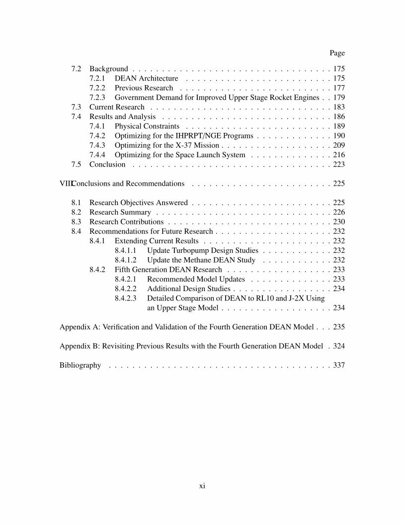
2 Background . . . . . . . . . . . . . . . . . . . . . . . . . . . . . . . . . . 1757.2.1 DEAN Architecture . . . . . . . . . . . . . . . . . . . . . . . . . 1757.2.2 Previous Research . . . . . . . . . . . . . . . . . . . . . . . . . . 1777.2.3 Government Demand for Improved Upper Stage Rocket Engines . . 179

7.3 Current Research . . . . . . . . . . . . . . . . . . . . . . . . . . . . . . . 1837.4 Results and Analysis . . . . . . . . . . . . . . . . . . . . . . . . . . . . . 186

7.4.1 Physical Constraints . . . . . . . . . . . . . . . . . . . . . . . . . 1897.4.2 Optimizing for the IHPRPT/NGE Programs . . . . . . . . . . . . . 1907.4.3 Optimizing for the X-37 Mission . . . . . . . . . . . . . . . . . . . 2097.4.4 Optimizing for the Space Launch System . . . . . . . . . . . . . . 216

7.5 Conclusion . . . . . . . . . . . . . . . . . . . . . . . . . . . . . . . . . . 223

VIII.Conclusions and Recommendations . . . . . . . . . . . . . . . . . . . . . . . . 225

8.1 Research Objectives Answered . . . . . . . . . . . . . . . . . . . . . . . . 2258.2 Research Summary . . . . . . . . . . . . . . . . . . . . . . . . . . . . . . 2268.3 Research Contributions . . . . . . . . . . . . . . . . . . . . . . . . . . . . 2308.4 Recommendations for Future Research . . . . . . . . . . . . . . . . . . . . 232

8.4.1 Extending Current Results . . . . . . . . . . . . . . . . . . . . . . 2328.4.1.1 Update Turbopump Design Studies . . . . . . . . . . . . 2328.4.1.2 Update the Methane DEAN Study . . . . . . . . . . . . 232

8.4.2 Fifth Generation DEAN Research . . . . . . . . . . . . . . . . . . 2338.4.2.1 Recommended Model Updates . . . . . . . . . . . . . . 2338.4.2.2 Additional Design Studies . . . . . . . . . . . . . . . . . 2348.4.2.3 Detailed Comparison of DEAN to RL10 and J-2X Using

an Upper Stage Model . . . . . . . . . . . . . . . . . . . 234

Appendix A: Verification and Validation of the Fourth Generation DEAN Model . . . 235

Appendix B: Revisiting Previous Results with the Fourth Generation DEAN Model . 324

Bibliography . . . . . . . . . . . . . . . . . . . . . . . . . . . . . . . . . . . . . . 337

xi

List of Figures

Figure Page

1.1 Pratt & Whitney RL10, credit NASA[1] . . . . . . . . . . . . . . . . . . . . . 3

1.2 The Dual-Expander Aerospike Nozzle Upper Stage Engine . . . . . . . . . . . 4

2.1 Liquid Rocket Engine Elements . . . . . . . . . . . . . . . . . . . . . . . . . 17

2.2 Cross-Section of a Truncated Aerospike Nozzle, taken from Martin [2] . . . . . 19

2.3 Typical Liquid Rocket Engine Cycles from Huzel and Huang[3], credit J. Hall[4] 21

2.4 Liquid Rocket Engine Design Process . . . . . . . . . . . . . . . . . . . . . . 22

2.5 Example Pressure Plot of a Gas Generator Cycle; redrawn from Humble [5] . . 24

2.6 Delta IV Upper Stage, credit NASA KSC [6] . . . . . . . . . . . . . . . . . . 31

2.7 Centaur Upper Stage, credit NASA KSC [7] . . . . . . . . . . . . . . . . . . . 32

2.8 SLS Upper Stage with Four RL10 Engines, credit The Boeing Corporation [8] . 35

2.9 SLS Upper Stage with Single J-2X Engine, credit The Boeing Corporation [8] . 37

2.10 X-37 Orbital Test Vehicle, credit US Air Force [9] . . . . . . . . . . . . . . . . 39

2.11 Rear View of X-37 including the AR2-3 Engine, credit US Air Force [10] . . . 40

2.12 DEAN Architecture, credit J. Hall (unpublished) . . . . . . . . . . . . . . . . 41

2.13 Example Aerospike Engines . . . . . . . . . . . . . . . . . . . . . . . . . . . 46

2.14 Second Generation DEAN Model . . . . . . . . . . . . . . . . . . . . . . . . 49

2.15 Comparison of First, Second, and Third Generation DEAN Geometry . . . . . 52

3.1 Original DEAN Geometry . . . . . . . . . . . . . . . . . . . . . . . . . . . . 61

3.2 DEAN Architecture . . . . . . . . . . . . . . . . . . . . . . . . . . . . . . . . 64

3.3 DEAN Geometry (dim in inches), credit D. Martin . . . . . . . . . . . . . . . 67

3.4 Updated DEAN Architecture . . . . . . . . . . . . . . . . . . . . . . . . . . . 71

3.5 Comparison of Simplified Geometry to Martin’s Original Geometry . . . . . . 72

3.6 Isp vs O/F, Original NPSS Model . . . . . . . . . . . . . . . . . . . . . . . . . 75

xii

Figure Page

3.7 Thrust vs O/F, Original NPSS Model . . . . . . . . . . . . . . . . . . . . . . . 76

3.8 Thrust vs O/F and Total Mass Flow, Original NPSS Model . . . . . . . . . . . 77

3.9 System-level Model of DEAN . . . . . . . . . . . . . . . . . . . . . . . . . . 78

3.10 Comparison of Fluid Mach Number Calculations . . . . . . . . . . . . . . . . 84

3.11 Isp vs O/F Ratio, System-level Model . . . . . . . . . . . . . . . . . . . . . . 85

3.12 Fluid Mach Numbers vs O/F Ratio, System-level Model . . . . . . . . . . . . 87

3.13 Detailed Isp vs O/F Ratio, System-level Model . . . . . . . . . . . . . . . . . 88

3.14 Detailed Chamber Pressure vs O/F Ratio, System-level Model . . . . . . . . . 89

3.15 Detailed Chamber Temperature vs O/F Ratio, System-level Model . . . . . . . 89

3.16 Isp vs O/F Ratio, Chamber Pressure, and Chamber Temperature, System-level

Model . . . . . . . . . . . . . . . . . . . . . . . . . . . . . . . . . . . . . . . 90

3.17 Vacuum Thrust vs Total Mass Flow, System-level Model . . . . . . . . . . . . 92

3.18 Vacuum Thrust vs Chamber Length, System-level Model . . . . . . . . . . . . 94

3.19 Comparison of Geometry for the scaled DEAN to the Original Geometry . . . 96

4.1 Key Radii in the DEAN Engine . . . . . . . . . . . . . . . . . . . . . . . . . . 101

4.2 Primary Elements of Revised DEAN Model . . . . . . . . . . . . . . . . . . . 104



5.3 Fourth Generation DEAN Model . . . . . . . . . . . . . . . . . . . . . . . . . 117

5.4 Key Radii in the DEAN Engine . . . . . . . . . . . . . . . . . . . . . . . . . . 117

5.5 Trade Study Baseline Design Geometry . . . . . . . . . . . . . . . . . . . . . 120

5.6 Total Mass Flow Variation with Vacuum Thrust for Five Expansion Ratios . . . 123

5.7 Chamber Pressure Variation with Thrust for Five Expansion Ratios . . . . . . . 125

5.8 Chamber Pressure Variation with Throat Area for Five Thrust Levels . . . . . . 126

xiii

Figure Page

5.9 Vacuum Specific Impulse Variation with Expansion Ratio for a Generic

LOX/LH2 Engine (Pc = 500 psia) . . . . . . . . . . . . . . . . . . . . . . . . 127

5.10 Vacuum Specific Impulse Variation with Expansion Ratio for Five Thrust Levels 128

5.11 Specific Impulse Variation with Molecular Weight for Five Thrust Levels . . . 129

5.12 Specific Impulse Variation with Oxidizer-to-Fuel Ratio for Five Expansion Ratios130

5.13 Total Engine Weight Variation with Throat Area for Five Thrust Levels . . . . . 131

5.14 Total Engine Weight Variation with Throat Area for Five Thrust Levels without

the Pressure Profile Converger . . . . . . . . . . . . . . . . . . . . . . . . . . 132

5.15 Total Engine Weight Variation with Expansion Ratio for Five Thrust Levels . . 133

5.16 Total Engine Weight Variation with Chamber Length for Five Expansion Ratios 133

5.17 Impact of Characteristic Length on DEAN Geometry . . . . . . . . . . . . . . 135

5.18 Total Engine Weight Variation with Characteristic Length for Five Expansion

Ratios . . . . . . . . . . . . . . . . . . . . . . . . . . . . . . . . . . . . . . . 136

5.19 Aerospike Thickness Variation with Characteristic Length for Five Expansion

Ratios . . . . . . . . . . . . . . . . . . . . . . . . . . . . . . . . . . . . . . . 137

6.1 DEAN Cooling Channels Variable Influence Chart . . . . . . . . . . . . . . . 149

6.2 DEAN Chamber Cooling Channels Variable Influence Chart . . . . . . . . . . 151

6.3 DEAN Aerospike Cooling Channels Variable Influence Chart . . . . . . . . . . 152

6.4 Chamber Wall Temperature Variation with Chamber Stations Adjustment . . . 153

6.5 Chamber Maximum Mach Number Variation with Chamber Stations Adjustment154

6.6 Channel Design Optimization Model . . . . . . . . . . . . . . . . . . . . . . . 156

6.7 Chamber Percent Melting Point Variation with Material for Various Throat

Areas and Thrust Levels . . . . . . . . . . . . . . . . . . . . . . . . . . . . . 164

6.8 Aerospike Percent Melting Point Variation with Material for Various Throat

Areas and Thrust Levels . . . . . . . . . . . . . . . . . . . . . . . . . . . . . 165

xiv

Figure Page

6.9 Chamber Structural Jacket Thickness Variation with Material Selection for

Various Expansion Ratios and Thrust Levels . . . . . . . . . . . . . . . . . . . 167

6.10 Chamber Structural Jacket Weight Variation with Material Selection for


6.11 Aerospike Structural Jacket Thickness Variation with Material Selection for


6.12 Aerospike Weight Variation with Material Selection for Various Expansion

Ratios and Thrust Levels . . . . . . . . . . . . . . . . . . . . . . . . . . . . . 169

6.13 Aerospike Tip Weight Variation with Material Selection for Various Expansion

Ratios and Thrust Levels . . . . . . . . . . . . . . . . . . . . . . . . . . . . . 170

6.14 LOX Plumbing Weight Variation with Material Selection for Various Expan-

sion Ratios and Thrust Levels . . . . . . . . . . . . . . . . . . . . . . . . . . . 171

6.15 LH2 Plumbing Weight Variation with Material Selection for Various Expan-

sion Ratios and Thrust Levels . . . . . . . . . . . . . . . . . . . . . . . . . . . 172

7.1 The Dual-Expander Aerospike Nozzle Upper Stage Engine . . . . . . . . . . . 175



7.4 X-37 Space Maneuvering Vehicle, credit US Air Force . . . . . . . . . . . . . 181

7.5 SLS Upper Stage Designs, credit The Boeing Corporation . . . . . . . . . . . 182

7.6 Fourth Generation DEAN Model . . . . . . . . . . . . . . . . . . . . . . . . . 184

7.7 Optimization Variable Influence Chart . . . . . . . . . . . . . . . . . . . . . . 193

7.8 Chamber Wall Temperature Variation with Throat Area . . . . . . . . . . . . . 193

7.9 Thrust-to-Weight Ratio Variation with Characteristic Length . . . . . . . . . . 194

7.10 Vacuum Specific Impulse Variation with Oxidizer-to-Fuel Ratio . . . . . . . . 195

7.11 LH2 Injector Face Pressure Drop Variation with Oxidizer-to-Fuel Ratio . . . . 196

xv

Figure Page

7.12 Wall Temperatures Variation with Throat Area for 30,000 lbf DEAN . . . . . . 198

7.13 Specific Impulse Variation with Expansion Ratio and Chamber Length for

30,000 lbf DEAN . . . . . . . . . . . . . . . . . . . . . . . . . . . . . . . . . 200

7.14 Darwin Configuration for the 30,000 lbf IHPRPT/NGE Case . . . . . . . . . . 202

7.15 Specific Impulse Variation with Thrust-to-Weight Ratio Pareto Front for the

30,000 lbf IHPRPT/NGE Case . . . . . . . . . . . . . . . . . . . . . . . . . . 203

7.16 30,000 lbf IHPRPT/NGE DEAN Optimal Design Geometry . . . . . . . . . . 204

7.17 Specific Impulse Variation with Thrust-to-Weight Ratio Pareto Fronts for

IHPRPT/NGE Cases . . . . . . . . . . . . . . . . . . . . . . . . . . . . . . . 205


X-37 DEAN Engine . . . . . . . . . . . . . . . . . . . . . . . . . . . . . . . . 213

7.19 X-37 DEAN Optimal Design Geometry . . . . . . . . . . . . . . . . . . . . . 213


SLS DEAN Engine . . . . . . . . . . . . . . . . . . . . . . . . . . . . . . . . 220

7.21 SLS DEAN Optimal Design Geometry . . . . . . . . . . . . . . . . . . . . . . 220

A.1 Fourth Generation DEAN Model . . . . . . . . . . . . . . . . . . . . . . . . . 235

A.2 ModelCenter Process Components . . . . . . . . . . . . . . . . . . . . . . . . 238

A.3 ModelCenter Converger . . . . . . . . . . . . . . . . . . . . . . . . . . . . . . 239

A.4 ModelCenter Surface of Revolution Component . . . . . . . . . . . . . . . . . 239

A.5 DEAN Preprocessing Components . . . . . . . . . . . . . . . . . . . . . . . . 240

A.6 Pressure Profile Converger Components . . . . . . . . . . . . . . . . . . . . . 248

A.7 Cooling Channel Pressure Study Results (without converger) . . . . . . . . . . 255

A.8 Cooling Channel Pressure Study Results (with converger) . . . . . . . . . . . . 256

A.9 Engine Cycle Analysis Components . . . . . . . . . . . . . . . . . . . . . . . 258

A.10 DEAN Geometry . . . . . . . . . . . . . . . . . . . . . . . . . . . . . . . . . 260

xvi

Figure Page

A.11 DEAN Chamber Volume Elements . . . . . . . . . . . . . . . . . . . . . . . . 265

A.12 Calculating Conical Nozzle Length . . . . . . . . . . . . . . . . . . . . . . . . 269

A.13 Comparison of Angelino Approximation to TDK (Martin Design Point) . . . . 275

A.14 Comparison of Angelino Approximation to TDK (Hall Design Point) . . . . . 276

A.15 Comparison of Angelino Approximation to TDK (Hall Design Point with

Expansion Ratio of 10) . . . . . . . . . . . . . . . . . . . . . . . . . . . . . . 276

A.16 Angelino Approximation Correction (Hall Design Point) . . . . . . . . . . . . 277

A.17 Angelino Approximation Correction (Hall Design Point with expansion ratio

of 10) . . . . . . . . . . . . . . . . . . . . . . . . . . . . . . . . . . . . . . . 278

A.18 Coordinating Angelino Approximation with Chamber Geometry . . . . . . . . 279

A.19 Cooling Channel Design - Cross-Section View [4] . . . . . . . . . . . . . . . . 281

A.20 Performance Sequence . . . . . . . . . . . . . . . . . . . . . . . . . . . . . . 292

A.21 Cross-Section of the DEAN Engine . . . . . . . . . . . . . . . . . . . . . . . 294

A.22 Pressure Level Plots Spreadsheet . . . . . . . . . . . . . . . . . . . . . . . . . 308

A.23 Example LOX Cycle Pressure Level Plot . . . . . . . . . . . . . . . . . . . . . 309

A.24 Geometry Sequence . . . . . . . . . . . . . . . . . . . . . . . . . . . . . . . . 310

A.25 Example Renderings from the Geometry Sequence . . . . . . . . . . . . . . . 311

A.26 Constraints Parallel Branch . . . . . . . . . . . . . . . . . . . . . . . . . . . . 312

A.27 LOX and LH2 Mach Number Sequences . . . . . . . . . . . . . . . . . . . . . 313

A.28 LOX RSM Actual vs Predicted Plots . . . . . . . . . . . . . . . . . . . . . . . 316

A.29 LOX RSM Actual vs Predicted Plots . . . . . . . . . . . . . . . . . . . . . . . 316

B.1 Geometry Comparison for First Generation DEAN Design . . . . . . . . . . . 329

B.2 Geometry for Second Generation DEAN Design . . . . . . . . . . . . . . . . . 331

B.3 Geometry Comparison for Third Generation DEAN Design . . . . . . . . . . . 336

xvii

List of Tables

Table Page

2.1 Thrust-to-Weight Range Based on Propellants . . . . . . . . . . . . . . . . . . 33

2.2 Key Performance Parameters for the SLS RL10 Rocket Engine Cluster [8, 11] . 36

2.3 Key Performance Parameters for the J-2X Rocket Engine [12, 13] . . . . . . . 36

2.4 Key Performance Parameters for the AR2-3 Rocket Engine [14] . . . . . . . . 39

3.1 Existing DEAN Design Results versus Requirements . . . . . . . . . . . . . . 62

3.2 Existing DEAN Design Point[2] . . . . . . . . . . . . . . . . . . . . . . . . . 68

3.3 Parametric Study over LH2 Pump 1 PR . . . . . . . . . . . . . . . . . . . . . 75

3.4 System-level DEAN Model Components . . . . . . . . . . . . . . . . . . . . . 79

3.5 Design of Experiments over O/F, Total Mass Flow, and Chamber Length . . . 82

3.6 Data Ranges for Speed of Sound Tables . . . . . . . . . . . . . . . . . . . . . 83

3.7 Parametric Study over O/F . . . . . . . . . . . . . . . . . . . . . . . . . . . . 86

3.8 Parametric Study over Total Mass Flow . . . . . . . . . . . . . . . . . . . . . 91

3.9 Parametric Study over Chamber Length . . . . . . . . . . . . . . . . . . . . . 93

3.10 Scaled DEAN Design Parameters . . . . . . . . . . . . . . . . . . . . . . . . 95

4.1 Assumed Performance Compared to Actual Performance for Previous DEAN

Generations . . . . . . . . . . . . . . . . . . . . . . . . . . . . . . . . . . . . 100

4.2 Updated DEAN Parametrization . . . . . . . . . . . . . . . . . . . . . . . . . 102

4.3 Fourth Generation DEAN Model Components . . . . . . . . . . . . . . . . . . 105


5.2 Trade Study Baseline Design . . . . . . . . . . . . . . . . . . . . . . . . . . . 121

5.3 Responses to Vacuum Thrust Trade Study Design . . . . . . . . . . . . . . . . 122

5.4 Responses to Throat Trade Study Design . . . . . . . . . . . . . . . . . . . . . 125

5.5 Responses to Expansion Ratio Trade Study Design . . . . . . . . . . . . . . . 126

xviii

Table Page

5.6 Comparison of DEAN and RL10B-2 Sizes . . . . . . . . . . . . . . . . . . . . 128

5.7 Responses to Oxidizer-to-Fuel Ratio Trade Study Design . . . . . . . . . . . . 129

5.8 Responses to Chamber Length Trade Study Design . . . . . . . . . . . . . . . 133

5.9 Responses to Characteristic Length Trade Study Design . . . . . . . . . . . . . 134

5.10 Design Variable Ranges . . . . . . . . . . . . . . . . . . . . . . . . . . . . . . 138

5.11 DEAN Simulation Reliability . . . . . . . . . . . . . . . . . . . . . . . . . . . 138

5.12 Comparison of RL10 Engine Family to DEAN Designs . . . . . . . . . . . . . 139

6.1 Generation 3 DEAN Materials Selection [4] . . . . . . . . . . . . . . . . . . . 143

6.2 Cooling Channel Design Variables . . . . . . . . . . . . . . . . . . . . . . . . 145

6.3 Cooling Channel Design Study Base Design . . . . . . . . . . . . . . . . . . . 147

6.4 Design Variables for Cooling Channel Design Study DOE 1 - Influence of

System Level Design Variables . . . . . . . . . . . . . . . . . . . . . . . . . . 149

6.5 Design Variables for Cooling Channel Design Study DOE 2 - Chamber

Channel Design Study . . . . . . . . . . . . . . . . . . . . . . . . . . . . . . 150

6.6 Design Variables for Cooling Channel Design Study DOE 3 - Aerospike

Channel Design Study . . . . . . . . . . . . . . . . . . . . . . . . . . . . . . 152

6.7 Cooling Channel Optimization Model Components . . . . . . . . . . . . . . . 157

6.8 Final Cooling Channel Design Variable Values . . . . . . . . . . . . . . . . . . 157

6.9 Cooling Channel Design Verification Results . . . . . . . . . . . . . . . . . . 159

6.10 Cooling Channel Design Comparison . . . . . . . . . . . . . . . . . . . . . . 160

6.11 Materials Studies Base Design . . . . . . . . . . . . . . . . . . . . . . . . . . 162

6.12 Materials Options for DEAN Components . . . . . . . . . . . . . . . . . . . . 163

6.13 Design Variables for Chamber Cooling Jacket Material Study . . . . . . . . . . 164

6.14 Design Variables for Aerospike Cooling Jacket Material Study . . . . . . . . . 165

6.15 Design Variables for Chamber Structural Jacket Material Study . . . . . . . . . 166

xix

Table Page

6.16 Design Variables for Aerospike Structural Jacket Material Study . . . . . . . . 168

6.17 Design Variables for LOX Plumbing Material Study . . . . . . . . . . . . . . . 170

6.18 Design Variables for LH2 Plumbing Material Study . . . . . . . . . . . . . . . 171

6.19 Generation 4 DEAN Design Materials Selection . . . . . . . . . . . . . . . . . 173

7.1 IHPRPT/NGE Requirements Compared to RL10 Performance . . . . . . . . . 180

7.2 SLS Designs Compared to RL10 Performance . . . . . . . . . . . . . . . . . . 183


7.4 DEAN Preassigned Parameters . . . . . . . . . . . . . . . . . . . . . . . . . . 188

7.5 DEAN Design Variables . . . . . . . . . . . . . . . . . . . . . . . . . . . . . 189

7.6 Base Design for IHPRPT/NGE Optimization Study . . . . . . . . . . . . . . . 191

7.7 Design Variables for IHPRPT/NGE Optimization Study DOE 1 - Trade Space

Exploration . . . . . . . . . . . . . . . . . . . . . . . . . . . . . . . . . . . . 192

7.8 Key Constraints for the DEAN Engine . . . . . . . . . . . . . . . . . . . . . . 194

7.9 DEAN Optimization Process . . . . . . . . . . . . . . . . . . . . . . . . . . . 197

7.10 Design Variables for IHPRPT/NGE 30,000 lbf Step 3 DOE . . . . . . . . . . . 199

7.11 Preassigned Parameters for IHPRPT/NGE 30,000 lbf Optimization Study . . . 200

7.12 IHPRPT/NGE Optimal Designs . . . . . . . . . . . . . . . . . . . . . . . . . 206

7.13 IHPRPT/NGE Optimal Designs Compared to RL10B-2 . . . . . . . . . . . . . 207

7.14 Base Design for X-37 Optimization Study . . . . . . . . . . . . . . . . . . . . 210

7.15 Preassigned Parameters for X-37 Optimization Study . . . . . . . . . . . . . . 211

7.16 X-37 Optimal Design . . . . . . . . . . . . . . . . . . . . . . . . . . . . . . . 214

7.17 X-37 Optimal Design Compared to RL10A-4 . . . . . . . . . . . . . . . . . . 215

7.18 Base Design for SLS Optimization Study . . . . . . . . . . . . . . . . . . . . 217

7.19 Preassigned Parameters for SLS Optimization Study . . . . . . . . . . . . . . 218

7.20 SLS Optimal Design compared to Baseline Designs . . . . . . . . . . . . . . . 221

xx

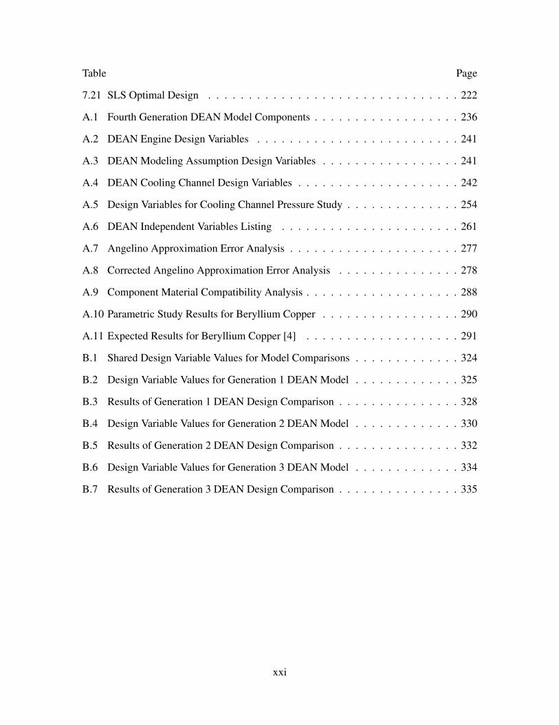
Table Page

7.21 SLS Optimal Design . . . . . . . . . . . . . . . . . . . . . . . . . . . . . . . 222

A.1 Fourth Generation DEAN Model Components . . . . . . . . . . . . . . . . . . 236

A.2 DEAN Engine Design Variables . . . . . . . . . . . . . . . . . . . . . . . . . 241

A.3 DEAN Modeling Assumption Design Variables . . . . . . . . . . . . . . . . . 241

A.4 DEAN Cooling Channel Design Variables . . . . . . . . . . . . . . . . . . . . 242

A.5 Design Variables for Cooling Channel Pressure Study . . . . . . . . . . . . . . 254

A.6 DEAN Independent Variables Listing . . . . . . . . . . . . . . . . . . . . . . 261

A.7 Angelino Approximation Error Analysis . . . . . . . . . . . . . . . . . . . . . 277

A.8 Corrected Angelino Approximation Error Analysis . . . . . . . . . . . . . . . 278

A.9 Component Material Compatibility Analysis . . . . . . . . . . . . . . . . . . . 288

A.10 Parametric Study Results for Beryllium Copper . . . . . . . . . . . . . . . . . 290

A.11 Expected Results for Beryllium Copper [4] . . . . . . . . . . . . . . . . . . . 291

B.1 Shared Design Variable Values for Model Comparisons . . . . . . . . . . . . . 324

B.2 Design Variable Values for Generation 1 DEAN Model . . . . . . . . . . . . . 325

B.3 Results of Generation 1 DEAN Design Comparison . . . . . . . . . . . . . . . 328





xxi

List of Symbols

α = conical nozzle half-angle (◦)

β = empirical exponent (range 0.6 - 0.667)

∆l = coolant channel wall thickness (in)

∆rthroat = difference between chamber and aerospike radii at the throat

∆T = change in temperature (R)

∆v = change in vehicle velocity (ft/s)

m = total mass flow (lbm/s)

mLH2 = LH2 mass flow (lbm/s)

mLOX = LOX mass flow (lbm/s)

Q = total heat transfer (BTU)

q = heat transfer per unit area (BTU/in2)

w = total propellant weight flow (lbf/s)

ε = expansion ratio

εaerospike = aerospike expansion ratio

ηp = pump efficiency

ηc∗ = combustion efficiency (frozen flow range: 1.0-1.15; equilibrium flow range: 0.9-

0.98)

xxii

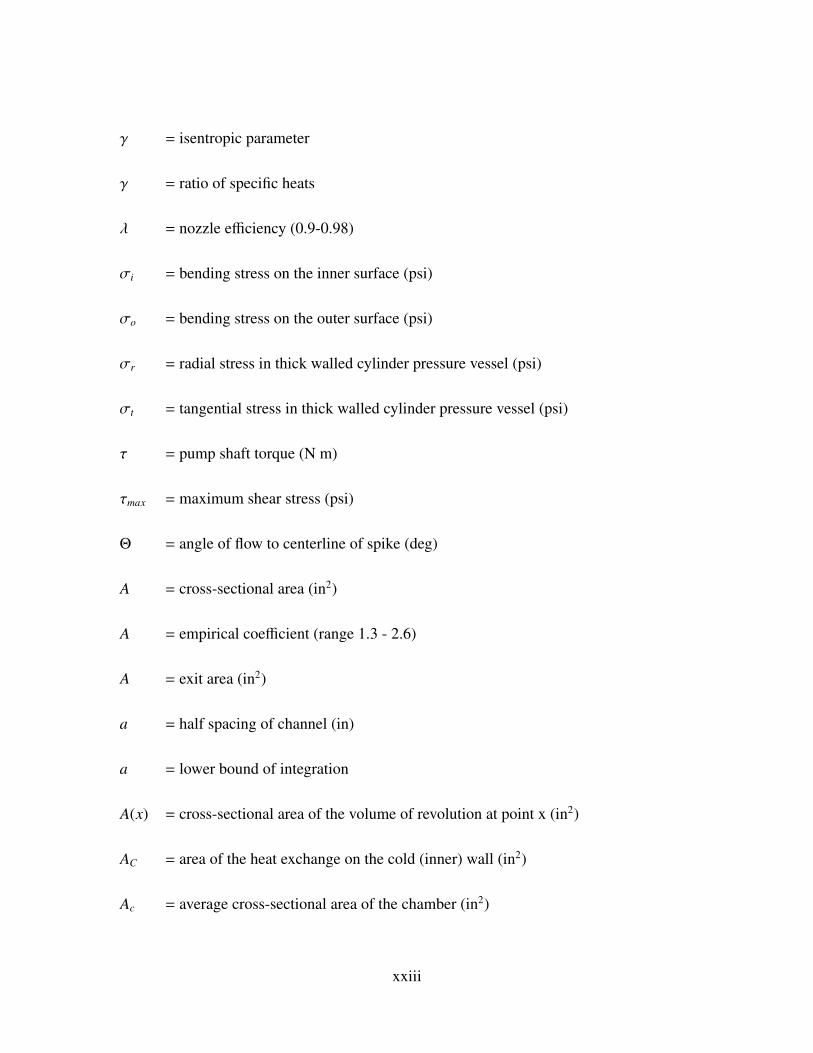
γ = isentropic parameter

γ = ratio of specific heats

λ = nozzle efficiency (0.9-0.98)

σi = bending stress on the inner surface (psi)

σo = bending stress on the outer surface (psi)

σr = radial stress in thick walled cylinder pressure vessel (psi)

σt = tangential stress in thick walled cylinder pressure vessel (psi)

τ = pump shaft torque (N m)

τmax = maximum shear stress (psi)

Θ = angle of flow to centerline of spike (deg)

A = cross-sectional area (in2)

A = empirical coefficient (range 1.3 - 2.6)

A = exit area (in2)

a = half spacing of channel (in)

a = lower bound of integration

A(x) = cross-sectional area of the volume of revolution at point x (in2)

AC = area of the heat exchange on the cold (inner) wall (in2)

Ac = average cross-sectional area of the chamber (in2)

xxiii

Ae = nozzle exit area (in2)

AH = area of the heat exchange on the hot (outer) wall (in2)

At = throat area (in2)

Ac throat = area of the chamber at the throat (in2)

Acv,i = cross-sectional area of cooling volume at ith station (in2)

A f low,i = combusted flow’s cross-sectional area at ith station (in2)

Ahxcv,i = area for heat exchange to cooling volume at ith station (in2)

Ahxnozz,i = area of heat exchange to aerospike nozzle at ith station (in2)

Ahx = area of heat exchange for chamber (in2)

aLH2,i = LH2 Mach number at ith station

aLOX,i = LOX Mach number at ith station

alt = altitude of orbit (ft)

AR = channel aspect ratio

B = empirical coefficient (range 0.6 - 0.667)

b = upper bound of integration

c∗ = characteristic exit velocity (ft/s)

cF = thrust coefficient (none)

ci = distance from neutral axis to inner fiber (in)

xxiv

co = distance from neutral axis to outer fiber (in)

De = nozzle exit diameter (in)

Dt = nozzle throat diameter (in)

e = distance from the centroid axis to the neutral axis (in)

F = total thrust (lbf)

Fm = momentum thrust (lbf)

Fp = pressure thrust (lbf)

Fvac = vacuum thrust (lbf)

Fcowl = thrust acting on the chamber lip (lbf)

finert = inert mass fraction

Fnondesign = thrust from the difference between exit and ambient pressure (lbf)

Fpressure = thrust from pressure acting on the surface area of the aerospike (lbf)

g0 = acceleration due to gravity on Earth (32.18 ft/s2)

h = heat transfer coefficient (BTU/in2 R)

hi = height of channel at ith station (in)

Hp = pump head pressure rise (m)

HTC = heat transfer coefficient from the cold (inner) side of the wall (BTU/in2 R)

HTH = heat transfer coefficient from the hot (outer) side of the wall (BTU/in2 R)

xxv

Hx = heat flow (R)

Isp vac = vacuum specific impulse (s)

Isp = specific impulse (s)

k = thermal conductivity of wall (BTU/in R)

L = length of frustum (in)

l = width (in)

L∗ = characteristic length (in)

Lc = chamber length (in)

lc = chamber length (in)

li = length of station = 0.2*lc (in)

Ln = conical nozzle length (in)

M = chamber Mach number

m f = final vehicle mass (lbm)

mi = initial vehicle mass (lbm)

Mx = bending moment (in lbf)

minert = mass of vehicle excluding propellant and payload (lbm)

mpay = mass of vehicle payload (lbm)

mplug = slope of the aerospike plug

xxvi

mprop = mass of consumed propellant (lbm)

mtp = mass of turbopump (kg)

mu = gravitational parameter = 1.40765 x 1016 ft3/s2 for Earth

MW = molecular weight of combustion products (lb/lb-mole)

N = number of points in the numerical integration

n = number of channels in cooling volume

Nr = pump rotational speed (rad/s)

O/F = oxidizer-to-fuel ratio

p∗ = throat pressure (psia)

pa = ambient pressure (psia)

pc = chamber pressure (psia)

pe = exit pressure (psia)

pi = fluid pressure at ith station (psia)

pi = internal pressure (psia)

po = external pressure (psis)

pamb = ambient pressure (psia)

Preq = required pump power (W)

Percent Weight Hardware = percent of engine mass accounted for by miscellaneous

hardware

xxvii

PRe = exit pressure ratio

Qin = total heat transfer into a system

Qout = total heat transfer out of a system

r1 = radius of base of frustum (in)

r2 = radius of top of frustum (in)

re = radius of exit area (in)

ri = inner radius of annulus (in)

ri = inside radius (in)

ri = radius of inner fiber (in)

ro = outer radius of annulus (in)

ro = outside radius (in)

ro = radius of the outer fiber (in)

rci,i = inner radius of the chamber at ith station (in)

rci = inner radius of the chamber (in)

rco,i = outer radius of the chamber at ith station (in)

rn,i−1 = radius of aerospike nozzle at (i-1)th station (in)

rn,i = radius of aerospike nozzle at ith station (in)

rplanet = radius of the planet (ft)

xxviii

rti = inner radius at throat (in)

S = shear force (lbf)

T0 = chamber temperature (R)

Ti = fluid temperature at ith station (R)

Tcool = temperature of coolant fluid (R)

TCW = temperature of the cold (inner) wall of the cooling channel (R)

THW = temperature of the hot (outer) wall of the cooling channel (R)

V = volume of of revolution (in3)

v∗ = throat velocity (ft/s)

V1 = volume 1 of chamber volume calculations (in3)



Vc = chamber volume (in3)

Vc = volume of cylinder (in3)

ve = exhaust velocity (ft/s)

V f = volume of frustum (in3)

V f h = volume of hollow frustum (in3)

vcir = circular orbital velocity (ft/s)

xxix

Vcv,i = volume of cooling volume at ith station (in3)

w = load per unit length (lbf/in)

wi = half width of channel at ith station (in)

Wchamber = weight of chamber (lb)

Whardware = mass of miscellaneous hardware (lb)

winit = initial half width of channel (in)

Wplumbing = weight of plumbing (lb)

Wspike = weight of aerospike (lb)

Wtotal = total engine weight (lb)

Wturbopumps = weight of turbopumps (lb)

x = position along the width of the beam (in)

xi = ith value of x

xi = percent of chamber length station is located at

xi−1 = (i-1)th value of x)

rti = inner throat radius (in)

rto = outer throat radius (in)

IHPRPT = Integrated High Payoff Rocket Propulsion Technology

LH2 = liquid hydrogen

xxx

LOX = liquid oxygen

NGE = Next Generation Engine

SLS = Space Launch System

xxxi

List of Source Code

A.1 Spike Materials Source Code . . . . . . . . . . . . . . . . . . . . . . . . . 243

A.2 Cooling Channels Design Source Code . . . . . . . . . . . . . . . . . . . . 246

A.3 Pressure Profile Converger Source Code . . . . . . . . . . . . . . . . . . . 250

A.4 Find Taget Isp Function Source Code . . . . . . . . . . . . . . . . . . . . . 252

A.5 Set Guess Lower Values Function Source Code . . . . . . . . . . . . . . . 253

A.6 Pressure RMSE Source Code . . . . . . . . . . . . . . . . . . . . . . . . . 257

A.7 DEAN Geometry Calculations . . . . . . . . . . . . . . . . . . . . . . . . 262

A.8 DEAN Estimated Pressure Level Calculations . . . . . . . . . . . . . . . . 269

A.9 Aerospike Thrust Calculation . . . . . . . . . . . . . . . . . . . . . . . . . 274

A.10 Cooling Jacket Bending Moment Function . . . . . . . . . . . . . . . . . . 282

A.11 Cooling Jacket Bending Stress Calculations . . . . . . . . . . . . . . . . . 282

A.12 Cooling Jacket Shear Stress Calculations . . . . . . . . . . . . . . . . . . . 283

A.13 Cooling Jacket Wall Temperature Calculations . . . . . . . . . . . . . . . . 286

A.14 Channels Component Average Function . . . . . . . . . . . . . . . . . . . 293

A.15 Tangential Stress in a Thick Walled Cylinder Function . . . . . . . . . . . 296

A.16 Radial Stress in a Thick Walled Cylinder Function . . . . . . . . . . . . . . 296

A.17 Calculate Wall Thickness Function . . . . . . . . . . . . . . . . . . . . . . 297

A.18 Frustum Volume Function . . . . . . . . . . . . . . . . . . . . . . . . . . 300

A.19 Volume of Revolution Volume Calculation . . . . . . . . . . . . . . . . . . 301

A.20 Aerospike Mass Calculations . . . . . . . . . . . . . . . . . . . . . . . . . 302

A.21 Turbopump Mass Calculations . . . . . . . . . . . . . . . . . . . . . . . . 304

A.22 Plumbing Mass Calculations . . . . . . . . . . . . . . . . . . . . . . . . . 304

A.23 Incorrect Miscellaneous Hardware Weight Calculation . . . . . . . . . . . 306

xxxii

A.24 Corrected Miscellaneous Hardware Weight Calculation . . . . . . . . . . . 306

A.25 Final Engine Thrust-to-Weight Calculation . . . . . . . . . . . . . . . . . . 306

A.26 GenericSOR Input Format . . . . . . . . . . . . . . . . . . . . . . . . . . 310

A.27 LOX Max Mach Source Code . . . . . . . . . . . . . . . . . . . . . . . . 317

A.28 Chamber Mach Number Source Code . . . . . . . . . . . . . . . . . . . . 319

A.29 Sanity Checks Source Code . . . . . . . . . . . . . . . . . . . . . . . . . . 321

xxxiii


STAGE ENGINE

I. Introduction

1.1 Research Motivation

Prices for space launches are literally astronomical. The cost to deliver payload to orbit

is estimated to be as much as $10,000 per pound [15]. A first class stamp to space (that is

delivery of up to 3.5 ounces by weight) would cost $2,200. Current launch costs to place

satellites in orbit costs hundreds of millions of dollars. In this time of budgetary constraints,

reliance placed on satellites for surveillance, navigation, communication, and meteorology

in the US also means there is demand for more efficient and cheaper improvements [16, 17].

At the heart of launch costs is the fundamental science and engineering of rocket

powered flight. Payloads represent only a small fraction of the gross lift-off weight

(GLOW) of current rockets. Improvements in propulsion performance, measured in

specific impulse (Isp) and the propulsion system’s thrust-to-weight ratio (T/W), can

dramatically increase payload fractions. Increased payload fractions reduce the size of

launch vehicles for a given payload leading to lower cost launch vehicles. Increased

payload fractions can also increase the size of payloads launched per mission, reducing

the per pound cost for fixed mission expenses, such as range and insurance costs. Taken

together, the savings can be significant.

Since 1996, the Department of Defense, NASA, and the aerospace propulsion industry

have been working to significantly improve rocket propulsion performance to realize these

benefits through two US Air Force programs. The first program is the Integrated High

Payoff Rocket Propulsion Technology (IHPRPT) program. One of the main goals of

1

the IHPRPT program was to double the thrust-to-weight ratio achieved by traditional

LOX/LH2 engines. DEAN research quantified this thrust-to-weight ratio requirement by

specifying a minimum value of 106.5 [2]. The second US Air Force program is the Next

Generation Engine (NGE) program. The NGE mission requirements include a vacuum

thrust between 25,000 lbf and 35,000 lbf and a minimum vacuum specific impulse of 465 s.

The NGE physical constraints include a maximum engine length of 90 in and a maximum

exit diameter of 73 in [18]. Taken together, the IHPRPT/NGE requirements represent a

significant improvement in weight and packaging over traditional expander cycle engines

such as the RL10, while requiring equal or better performance in terms of thrust and specific

impulse. Government estimates predict these performance increases will increase payload

mass by 22% and decrease launch costs by 33% for expendable launch vehicles.[19]

Two additional US government programs could benefit from advances in rocket engine

design. The US Air Force X-37 is a reusable space plane designed to test various spaceflight

hardware and technologies. Its small size and reusability call for compact rocket engines

able to operate many times before replacement. The X-37 is currently outfitted with an

AR2-3 engine producing 6,600 lbf of thrust and measuring just 32 in long with an outer

radius of 10 in [14, 20, 21]. NASA’s Space Launch System (SLS) is a shuttle-derived

super-heavy lift human-rated launch system which is still in the design phase. Four upper

stage configurations are being considered for the SLS including a design powered by four

RL10 engines and one powered by a single J-2X, an improved version of the gas generator

powered J-2 engine from the Apollo program. The RL10 design provides a vacuum thrust

of 99,000 lbf and a vacuum specific impulse of 462.5 s, with a thrust-to-weight ratio of

37.3 and the J-2X design provides a vacuum thrust of 294,000 lbf and a vacuum specific

impulse of 448 s, with a thrust-to-weight ratio of 55 [8, 12, 22].

Achieving the significant gains in performance required by these programs will take

more than incremental improvements in rocket engine technology. For decades the thrust-

2

to-weight ratio of high powered liquid rocket engines, including Pratt & Whitney’s upper

stage RL10 shown in Figure 1.1, has been relatively constant with respect to propellant

selection. Engines powered by liquid hydrogen/liquid oxygen have historically had thrust-

to-weight ratios between 41 and 61. Engines powered by RP-1/liquid oxygen have

historically had thrust-to-weight ratios between 71 and 102. This trend is present across a

variety of thrust levels and designs.[23]

Figure 1.1: Pratt & Whitney RL10, credit NASA[1]

The Air Force Institute of Technology (AFIT) is researching a modification to a

traditional upper stage engine architecture as a means of breaking through this performance

barrier. The result of this research is the Dual-Expander Aerospike Nozzle (DEAN) upper

stage engine. The DEAN, shown in Figure 1.2, uses two novel design choices. The first is

the use of separate expander cycles for the fuel and the oxidizer. In a traditional expander

cycle, the fuel is pumped through a cooling jacket for the chamber and nozzle. The energy

transferred to the fuel from cooling the chamber and nozzle is then used to drive the turbine

3

turning both the fuel and oxidizer pumps before the fuel is introduced into the chamber [5].

In the DEAN, the fuel and oxidizer each drive their own turbines to power their own pumps.

The second novel design choice of the DEAN is the use of an aerospike, or plug,

nozzle. Aerospike nozzles run through the middle of the rocket’s propellant flow and up

into the chamber, leaving the ambient atmosphere to form the outer boundary for the flow.

The interaction with the ambient atmosphere gives aerospike nozzles automatic altitude

compensation, making them more efficient over a range of altitudes. Similar bell nozzles

operate most efficiently at their specific design altitude [24]. The use of an aerospike

nozzle provides a second, physically separate cooling loop from the chamber for use in the

fuel expander cycle. This second cooling loop simplifies the propellant feed system and

increases the surface area inside the chamber used to drive the turbomachinery, providing

for correspondingly increased power to the pumps. The increased pump power leads to

increased chamber pressure, and in turn increased engine performance.

Figure 1.2: The Dual-Expander Aerospike Nozzle Upper Stage Engine

4

The DEAN’s unique architecture offers a number of advantages. The increased

chamber pressure yields smaller engines, in terms of both weight and physical dimensions,

for similar levels of thrust and specific impulse. The separate expander cycles also ensure

the fuel and oxidizer remain physically separated until entering the combustion chamber,

eliminating one of the more catastrophic failure modes in traditional expander cycles,

namely failure of an inter-propellant seal. The DEAN architecture is also a forerunner to

a similar boost stage architecture, where the aerospike nozzle’s global performance could

result in even greater performance gains [2, 25–27].

The DEAN architecture is not without its challenges, though. The LOX cycle requires

a turbine material to operate in an oxygen environment. Materials surveys at AFIT have

shown Inconel 718 provides both satisfactory oxygen resistance and suitable mechanical

performance for use in both the pump and the turbine in the LOX cycle [26, 27]. Also, the

expansion ratio of aerospike nozzles is limited by the ratio of the chamber area at the throat

to the throat area [24]. Due to this limit, aerospike nozzles generally need larger chamber

diameters to reach useful expansion ratios, potentially limiting the range of engines which

offer improved thrust-to-weight while also delivering the required specific impulse.

A number of simulation models of the DEAN have been developed at AFIT for a

single design targeting the IHPRPT program requirements demonstrating the feasibility of

the DEAN architecture. The primary model is a complete cycle model written in NASA’s

Numerical Propulsion System Simulation (NPSS).[2, 25, 26]

1.2 Problem Statement

The DEAN has been proposed as an improved upper stage rocket engine architecture

offering increased performance in a physically compact package. Addressing this proposal

requires answering the following questions.

• What are the operational limits of the DEAN architecture in terms of thrust and

specific impulse?

5

• What are the limiting constraints of the DEAN architecture?

• How does the DEAN compare to single expander cycle engines like the RL10 in

terms of specific impulse, thrust-to-weight ratio, and size?

• For what missions does the DEAN offer significant advantages over traditional upper

stage engines?

1.3 Research Objective

The objective of this research is to determine the viability of the DEAN architecture

by finding those missions and designs for which the DEAN has a competitive advantage

over traditional upper stage engines. This objective can be broken down into three sub-

objectives. The first sub-objective is to address the parametrization of the DEAN model.

On the practical level, the simulation must implement parametrization of the cycle model

in NPSS. On the architecture level the simulation must select a set of parameters which

fully defines the design and provides for robust execution of the model. The second sub-

objective is verifying the models used in the research and DEAN architecture. The third

sub-objective is comparing the performance of the DEAN to traditional upper stage engines

for a selection of missions, both current and proposed, in order to collect the data necessary

to satisfy the overall research objective.

1.4 Method Overview

This research built upon the initial work at AFIT on the DEAN. It extended the existing

cycle model of the DEAN to enable running parametric and optimization studies. The

research occurred in five phases. The first phase covered the development of a proof of

concept parametric system model of the DEAN. This first model was used to demonstrate

the utility of parametric modeling in rocket engine design by providing an improved design

from the results of parametric studies. These initial results led to extending the prototype

model to calculate improved performance and engine weight estimates.

6

The second phase involved the development of a new system level DEAN model

integrating the lessons learned from the previous efforts. The resulting model had the

necessary fidelity, flexibility, and reliability to address the research questions in the previous

section. The improved model was used throughout the remainder of this research starting

with phase three. The third phase was a detailed verification of the DEAN models and

architecture. The verification process included review and comparison of model source

code to engineering principles and parametric studies comparing the DEAN’s responses to

rocket engineering theory and the RL10 family of expander cycle engines.

With the model and architecture verified, the remaining phases focused on optimizing

the DEAN and comparing it to existing engines for a the IHPRPT/NGE, X-37, and SLS

missions. The fourth phase looked at the materials selection for the DEAN to find a

materials selection yielding consistently low weight engines across a wide range of designs.

Finally, the fifth phase covered a series of optimization studies of the DEAN for the three

selected missions and compared the DEAN’s performance and size to traditional upper

stage engines.

1.5 Research Contributions

1. A method for parametrically modeling rocket engines in NASA’s Numerical

Propulsion System Simulation (NPSS) was demonstrated including calculation of

initial estimates for key parameters in the NPSS model and calculation of fluid Mach

numbers in the cooling channels. The ability to develop a parametric model with the

required fidelity, flexibility, and reliability is essential for conceptual design studies

of new rocket engine architectures such as the DEAN.

2. The DEAN architecture was verified through a series of parametric studies. These

studies confirmed the validity of the DEAN architecture and demonstrated the

increased performance generated by the dual-expander cycles.

7

3. The materials selection proposed in previous research was refined to support a wide

variety of missions and engine designs.

4. An optimization process for DEAN engines using the DEAN simulation was

developed and demonstrated. This optimization process takes mission specific

requirements and constraints and yields a Pareto set of designs, trading off specific

impulse and thrust-to-weight ratio.

5. Optimal DEAN engine designs were found for three IHPRPT/NGE cases, the X-37

space plane, and two upper stage configurations of the SLS. These optimal designs

were compared to existing and proposed engines to demonstrate the benefits of the

DEAN architecture.

1.6 Dissertation Overview

The dissertation developed from this research follows the scholarly article format.

The document is divided into eight chapters and two appendices. Chapter 2 contains the

engineering and technical material relevant to the research. The material in Chapter 2 is

broken into four sections. The first section covers rocket powered propulsion with emphasis

on liquid rocket engines, including design and modeling. The second section documents

three US government programs involving advanced rocket propulsion: the US Air Force

IHPTRPT and NGE programs, the US Air Force X-37 space plane, and NASA’s SLS. The

third section presents a detailed review of previous research related to the DEAN. The

fourth and final section covers engineering optimization including terminology, problem

definition, and optimization algorithms.

Chapter 3 covers the initial parametrization of the DEAN and early conclusions from

the resulting parametric model. The parametric studies varied oxidizer-to-fuel ratio, total

mass flow, and chamber length. The DEAN can achieve 50,000 lbf vacuum thrust and 489 s

vacuum specific impulse with an oxidizer-to-fuel ratio of 6.0, a total propellant weight flow

8

of 104 lb/s (a reduction of 14%), and an engine length of 27.9 in (a reduction of over 25%

from the original design), a significant weight savings. These results validated both the

parametric modeling approach of the research and the DEAN architecture. Chapter 3 was

submitted to and published in the AIAA Journal of Spacecraft and Rockets (see reference

[27]).

Chapter 4 documents the final DEAN system model. The chapter opens with a detailed

review of the need for an improved system model emphasizing the narrow trade space

size and insufficient reliability of the initial parametric model and the models following it.

Chapter 4 continues by describing the improvements in the new system model. It concludes

with an overview of the system model’s structure and execution.

Chapter 5 presents the verification of the final system model and DEAN architecture.

Parametric studies using the system model verified the DEAN architecture conforms to

rocket engine theory while exceeding the RL10’s performance. Improvements in the new

model led to designs which can match the RL10’s vacuum specific impulse of 465 seconds

while retaining thrust-to-weight ratios in excess of 135 and chamber pressures of greater

than 1500 pounds psia. These designs are compact, ranging in length from 27 to 38 inches.

The parametric studies also demonstrated the new model is flexible and robust, with 98.7%

of the specified designs converging successfully on a design point. Chapter 5 was submitted

to the AIAA Journal of Propulsion and Power.

Chapter 6 covers the optimization of the cooling channel geometry for the DEAN

and the selection of materials for the DEAN designed to yield consistently low weight

engines across a wide range of designs. The cooling channel optimization process was

used in support of the materials study in Chapter 6 and later optimization studies. The

materials study confirmed the following findings from previous research: the aerospike tip

material selection has little influence on the engine’s thrust-to-weight ratio, the chamber

cooling jacket should be manufactured from silicon carbide, the LOX plumbing should

9

be manufactured from INCONEL 718, and the LH2 plumbing should be manufactured

from INCOLOY 909. The material study found updated material selections for the

aerospike cooling jacket (silicon carbide), chamber structural jacket (INCONEL 718), and

the aerospike structural jacket (INCOLOY 909).

Chapter 7 presents the optimized DEAN engine for three US government missions.

For the IHPRPT/NGE programs, the optimized design delivered 35,000 lbf of vacuum

thrust and 469.4 seconds of vacuum specific impulse with a thrust-to-weight ratio of 127.2

in an engine that is one quarter the size of a comparable RL10. For the X-37 mission, the

optimized design operated at 6,600 lbf of vacuum thrust and has a vacuum specific impulse

of 457.2 seconds with a thrust-to-weight ratio of 107.5. For the SLS, the optimized design

produced a vacuum thrust of 100,000 lbf and a vacuum specific impulse of 465.9 seconds

with a thrust-to-weight ratio of 110.2. When configured in a cluster of three engines, the

DEAN matched the J2-X vacuum thrust with a 4% increase in specific impulse while more

than doubling the J2-X’s thrust-to-weight ratio. Chapter 7 was submitted to the AIAA

Journal of Spacecraft and Rockets.

Chapter 8 concludes the dissertation by covering the research results, contributions,

and recommendations for future work. Following Chapter 8 are two appendices. The first

appendix covers the verification and validation of the individual analysis modules making

up the final system model. The second appendix reevaluates the three designs from previous

DEAN research using the final system model to confirm the results of earlier research.

10

II. Background

This chapter covers the engineering and technical material relevant to the research

presented in this work. The first section covers rocket powered propulsion with an

emphasis on liquid rocket engines, rocket design, and rocket modeling. The second section

documents three US government programs involving advanced rocket propulsion: the

US Air Force Integrated High Payoff Rocket Propulsion Technology (IHPRPT) and Next

Generation Engine (NGE) programs, the US Air Force X-37 space plane, and NASA’s

Space Launch System (SLS). The third section presents a detailed review of previous

research related to the DEAN. The fourth and final section covers engineering optimization

including terminology, problem definition, and optimization algorithms.

2.1 Rocket Propulsion

2.1.1 Rocket Fundamentals.

Rockets belong to the “jet” class of propulsion systems. “Jet” systems impart a force,

the thrust, on bodies by ejecting matter. In rockets, the ejected matter is carried with

the rocket and is called the propellant(s). For chemical rockets, such as those used in

space launch vehicles, the propellants are also the source of the energy for the rocket [24].

Spacecraft use the thrust provided by rockets to perform a number of functions related to

their motion (launch, orbit insertion, orbit maintenance/maneuvering) and rotation (attitude

control). The spacecraft launch process carries the spacecraft from a planetary surface to

orbit and orbit insertion transfers a spacecraft from its initial orbit to its operational orbit.

Orbit maintenance is the process of keeping a spacecraft in the required orbit and orbit

maneuvering is the process of transitioning to a new orbit. Attitude control is the process

of maintaining the required spacecraft pointing [5].

11

Chemical rockets are classified into three broad categories based on the type of

propellants used: liquid, solid, and hybrid. Liquid rockets use liquid propellants stored

in tanks and are either bi-propellant or mono-propellant. Bi-propellant systems use the

combustion of a fuel and oxidizer as their energy source. Mono-propellant systems use the

energy from a chemical decomposition of a single propellant. Feed systems transport the

propellants to a combustion chamber where they chemically react to release the necessary

energy to eject the products. Liquid rocket engines can have very high performance and

control, in some cases including restart capability, but have a high degree of complexity.

Solid rockets combine the propellants ahead of time and store them in solid form inside

of the combustion chamber. Solid rockets offer simplicity and small size, but have lower

performance than liquid rockets and cannot be shut down once they have been started.

Finally, hybrid rockets combine traits from both liquid and solid rockets. Generally, hybrid

rockets utilize a solid fuel stored in the chamber and a liquid or gaseous oxidizer stored in

a tank. Like liquid rockets, a feed system is used to transport the oxidizer from the tank

to the chamber. Hybrid rockets’ complexity, performance, and size fall between those of

liquid and solid rockets, while their safety is generally seen as far better than either that of

liquid or solid rockets [5, 24].

Three key performance values are used to describe a rocket propulsion system. The

first performance value is its thrust (F). As discussed above, the thrust is the force imparted

by the rocket on the body it is propelling. The second performance value is its specific

impulse (Isp). Specific impulse is the ratio of a rocket’s thrust to its propellant weight flow

rate, a measure of fuel economy. The third performance value is the rocket’s thrust-to-

weight ratio (T/W). The thrust-to-weight ratio is the ratio of a rocket propulsion system’s

thrust to the propulsion system’s weight. In liquid and hybrid rockets, the propulsion

system’s weight includes the feed system weight [5, 24].

12

A rocket’s thrust comes primarily from two sources: momentum thrust (Equation (2.1))

and pressure thrust (Equation (2.2)). The total thrust, shown in Equation (2.3), is the sum

of these two sources times a nozzle efficiency rating (λ) used to account for various losses

in the nozzle. The rocket’s exhaust velocity (ve) and exit pressure (pe) are tightly coupled to

the expansion of the rocket’s nozzle. These terms also have an inverse relationship where

increasing the rocket’s expansion leads to increased exhaust velocity with decreased exit

pressure and vice versa. Due to their inverse relationship, maximizing a rocket’s thrust is

not just a matter of maximizing the exhaust velocity and exit pressure. Instead, the maxi-

mum thrust corresponds to designs with exit pressures equal to the ambient pressure (pa)

[5, 24].

Fm = mve (2.1)

Fp = (pe − pa)Ae (2.2)

F = λ[mve + (pe − pa)Ae] (2.3)

A rocket exhaust flow is said to be ideally expanded when the exit pressure equals the

ambient pressure giving the maximum thrust. For steady, supersonic flow (no separation

from the nozzle) the exit pressure is constant for a given engine plus nozzle combination

and the flow is only ideally expanded at a single altitude. At all other altitudes, the flow is

either over or under expanded at other altitudes. Over expansion occurs when the engine

is operating below its optimal altitude and the ambient pressure is greater than the exit

pressure. This condition makes the effective exit area smaller than the actual exit area and

can cause the flow to separate from the nozzle. Under expansion occurs when the engine

operates above its optimal altitude and the ambient pressure is less than the exit pressure.

Under expanded flows fan out past the nozzle exit area. In both conditions, the thrust is

13

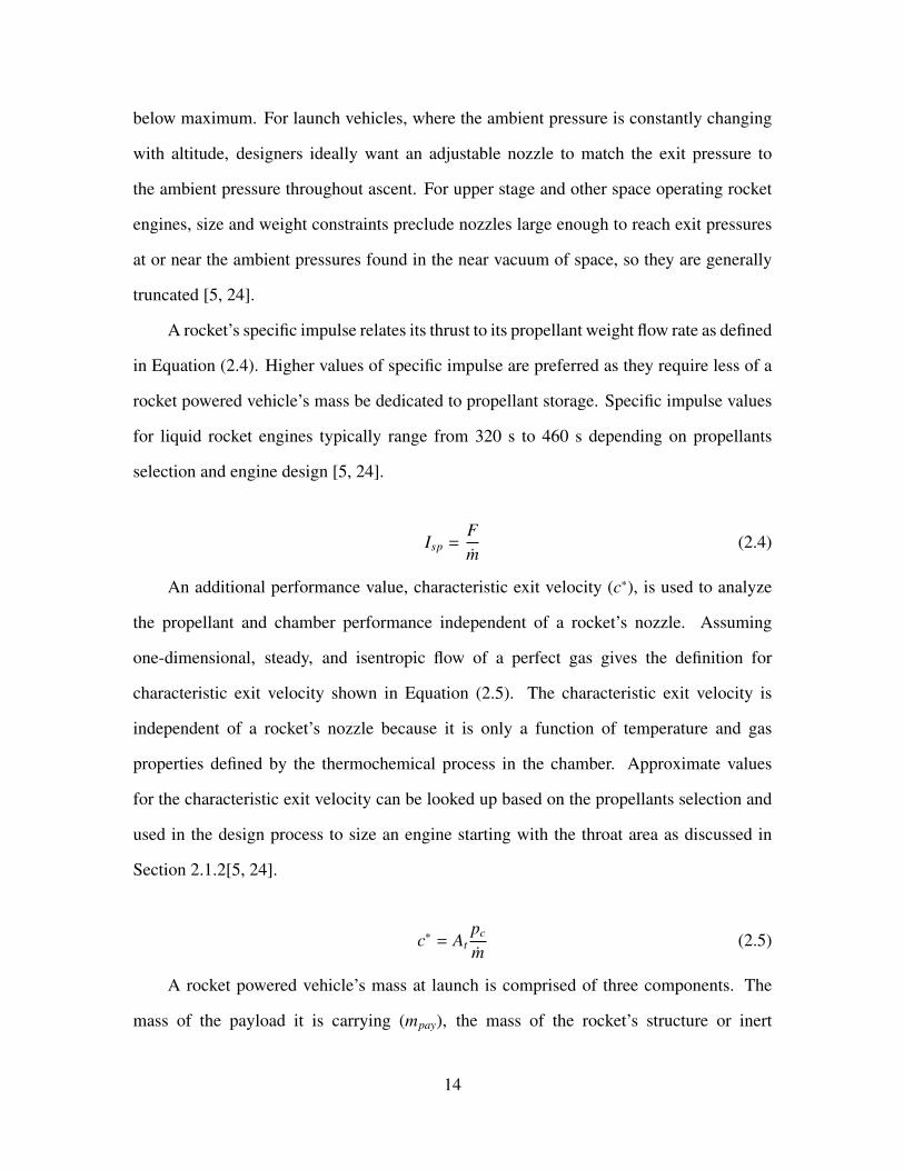
below maximum. For launch vehicles, where the ambient pressure is constantly changing

with altitude, designers ideally want an adjustable nozzle to match the exit pressure to

the ambient pressure throughout ascent. For upper stage and other space operating rocket

engines, size and weight constraints preclude nozzles large enough to reach exit pressures

at or near the ambient pressures found in the near vacuum of space, so they are generally

truncated [5, 24].

A rocket’s specific impulse relates its thrust to its propellant weight flow rate as defined

in Equation (2.4). Higher values of specific impulse are preferred as they require less of a

rocket powered vehicle’s mass be dedicated to propellant storage. Specific impulse values

for liquid rocket engines typically range from 320 s to 460 s depending on propellants

selection and engine design [5, 24].

Isp =Fm

(2.4)

An additional performance value, characteristic exit velocity (c∗), is used to analyze

the propellant and chamber performance independent of a rocket’s nozzle. Assuming

one-dimensional, steady, and isentropic flow of a perfect gas gives the definition for

characteristic exit velocity shown in Equation (2.5). The characteristic exit velocity is

independent of a rocket’s nozzle because it is only a function of temperature and gas

properties defined by the thermochemical process in the chamber. Approximate values

for the characteristic exit velocity can be looked up based on the propellants selection and

used in the design process to size an engine starting with the throat area as discussed in

Section 2.1.2[5, 24].

c∗ = Atpc

m(2.5)

A rocket powered vehicle’s mass at launch is comprised of three components. The

mass of the payload it is carrying (mpay), the mass of the rocket’s structure or inert

14

mass (minert), and the mass of the propellant made up of both the fuel and the oxidizer

(mprop). The relationship among these masses is governed by the rocket equation, shown

in Equation (2.6). In the rocket equation, ∆v is the change in the vehicle’s velocity

(discussed in more detail below) and ve is the propellant exhaust velocity which affects

the rocket’s performance. The masses are related by initial mass (mi) and final mass (m f ).

Equation (2.7) and Equation (2.8) show the relationship between the mass terms of the

rocket equation and the payload, inert and propellant masses [5].

∆v = −veln(m f

mi

)(2.6)

mi = m f + mprop (2.7)

m f = mpay + minert (2.8)

In addition to the actual mass values, the inert mass fraction can reveal important

insights into a rocket’s performance, shown in Equation (2.9). The inert mass fraction

represents the structural efficiency of a rocket powered vehicle with smaller values

representing more efficient structures. Traditional expendable launch vehicles have inert

mass fractions in the range of 0.08 to 0.12. The inert mass fraction can be combined with

a rocket’s specific impulse to predict the required propellant needed to achieve a specified

∆v [5].

finert =minert

mprop + minert(2.9)

As mentioned above, the rocket equation relates the initial and final masses and the

propellant exhaust velocity to the change in the vehicle’s velocity. This change in velocity is

the primary effect of the rocket and is what enables launch vehicles to propel their payloads

into orbit. In order to achieve orbit, the payload must be accelerated to the required orbital

15

velocity. Many payloads are placed into circular orbits. Equation (2.10) gives the orbital

velocity for circular orbits, where µ is a gravitational parameter for the planet, rplanet is the

radius of the planet, and alt is the altitude of the orbit. As an example, the orbital velocity

for circular orbit at approximately 124 mi (656,170 ft) is 25,540 ft/s [28].

vcir =

√µ

rplanet + alt(2.10)

While providing sufficient ∆v to reach orbital velocity is a requirement to reach orbit,

in reality it is not sufficient. Launch vehicles experience a number of velocity losses during

launch. These losses include gravity, atmospheric drag, and the expenses related to steering

the vehicle during launch. These losses average between 3280 and 6560 ft/s for launches

to Low Earth Orbits. Thus the required ∆v for a rocket powered launch vehicle is the sum

of the orbital velocity and the losses experienced during launch. For launch vehicles with

multiple stages, each stage will have its own required ∆v determined by target velocities

for the staging points in the launch profile and the losses the stage will encounter [5].

2.1.2 Liquid Rocket Engines.

Liquid rocket engines are a class of chemical rockets which use liquid propellants to

create chemical reactions converting thermochemical potential to kinetic energy to drive the

propellants out of the rocket and create the thrust. Figure 2.1 shows the primary elements

of liquid rocket engines. Bi-propellant liquid rockets use two propellants, an oxidizer and

a fuel, to create the required chemical reaction. Mono-propellants use a single propellant,

sometimes with a catalyst. In either case, the propellants are transferred from the storage

system, usually referred to as the tanks, to the injector face by the propellant feed system.

The feed system varies by engine cycle, and includes any required pumps, turbines, feed

lines, or pressurization fluids used to transfer the propellants to the combustion chamber.

The injector introduces the propellants into the chamber and separates the propellants from

the combustion process ensuring the required mixing takes place to support the combustion

16

process. The chemical reaction occurs in the combustion chamber itself driving the process.

This reaction forces the propellants, in the form of the reaction products, out of the engine

through the throat. The chamber cross-section contracts as the propellants approach the

throat, speeding up the flow from sub-sonic velocities to Mach 1 at the throat. The flow

then enters the nozzle turning the flow to direct the momentum. The flow continues to

accelerate through the diverging nozzle until reaching the exit plane and leaving the engine

[5].

Figure 2.1: Liquid Rocket Engine Elements

The length of a rocket’s nozzle depends on two key factors: the type of nozzle

(discussed below) and its expansion ratio, shown in Equation (2.11). The expansion ratio,

or area ratio, is the ratio of nozzle’s exit area to its throat area and is a measure of a nozzle’s

expansion. All other things being equal, larger expansion ratios lead to longer, and more

massive, nozzles. But, this extra mass usually comes with significant improvements in

specific impulse [5].

ε =Ae

At(2.11)

17

Traditional nozzle types are generally named after their shape. The simplest nozzle

type is the conical nozzle, described by the half angle (α) of their cone. While still used on

relatively small rockets such as missiles, the conical nozzle is not widely used on launch

vehicle rocket engines. The most common nozzle used on launch vehicle engines is the bell

nozzle, named after its rounded, bell like shape. Bell nozzles offer higher efficiency than

conical nozzles, especially at their design altitude, and are still relatively easy to design and

manufacture. Full length bell nozzles are usually too long to be practical, so they are often

shortened. The actual length is usually described in terms of the percent of a full length

conical nozzle with a 15◦ half angle at the same expansion ratio. For example, an 80% bell

nozzle would be 20% shorter than the comparable conical nozzle [24].

An alternative to conical and bell nozzles is the aerospike or plug nozzle. A cross-

section of a truncated aerospike nozzle is shown in Figure 2.2. Aerospike nozzles are a

center body in the combusted propellant flow often forming the inner wall of the chamber.

The ambient atmosphere forms the outer boundary for the flow for these nozzles. The

combusted propellant flow expands against the aerospike nozzle radially outward to match

ambient pressure at each location in the nozzle flow field. The interaction with the

ambient atmosphere gives aerospike nozzles altitude compensation ability, making them

more efficient as altitude changes for the rocket than similar bell nozzles [24].

Aerospike nozzles can be quite long, often equaling the length of conical nozzles with

half angles between 10◦ and 12◦. The expansion ratio of aerospike nozzles is limited by the

chamber geometry as shown in Equation (2.12) [4, 24]. Due to this limit, aerospike nozzles

generally need larger chamber diameters to reach useful expansion ratios, potentially

limiting the range of engines offering acceptable thrust-to-weight while also delivering the

required specific impulse.

εaerospike =Ac throat

At(2.12)

18

Figure 2.2: Cross-Section of a Truncated Aerospike Nozzle, taken from Martin [2]

The chemical reaction driving liquid rocket engines generates a substantial amount

of heat which must be managed to avoid damaging the engine. Four cooling approaches

are commonly used to manage this heat. Humble discusses the four approaches to rocket

engine cooling in Space Propulsion Analysis and Design [5]. The first is simple radiation

cooling. In radiation cooling, there is no active cooling system. Instead the structure

of the engine is allowed to heat up until it begins to radiate its heat into space. This

approach is generally used for small engines with low operating temperatures and short

burn durations in vacuum environments. The second approach is ablative cooling. In

ablative cooling, the chamber is lined with an expendable material ablating as the engine

operates. This approach is relatively simple, but adds weight to the engine and slightly

reduces the specific impulse as additional mass is injected into the exhaust without any

additional energy. Ablative cooling also limits the lifetime of the engine to the time it

takes to fully ablate the expendable liner. The third approach is regenerative cooling. In

regenerative cooling, the propellant feed system is integrated into the chamber structure

circulating cold propellant through a heat exchanger. The propellant then absorbs some

of the heat from the engine before injection into the chamber, keeping the engine within

19

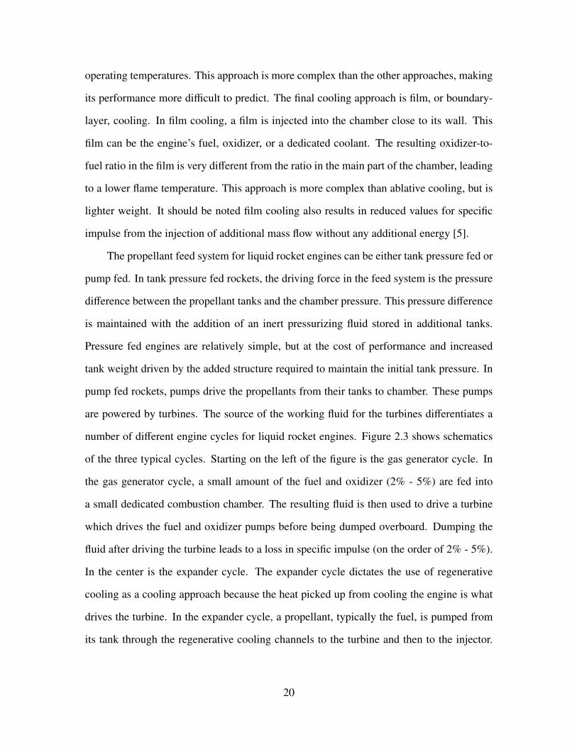
operating temperatures. This approach is more complex than the other approaches, making

its performance more difficult to predict. The final cooling approach is film, or boundary-

layer, cooling. In film cooling, a film is injected into the chamber close to its wall. This

film can be the engine’s fuel, oxidizer, or a dedicated coolant. The resulting oxidizer-to-

fuel ratio in the film is very different from the ratio in the main part of the chamber, leading

to a lower flame temperature. This approach is more complex than ablative cooling, but is

lighter weight. It should be noted film cooling also results in reduced values for specific

impulse from the injection of additional mass flow without any additional energy [5].

The propellant feed system for liquid rocket engines can be either tank pressure fed or

pump fed. In tank pressure fed rockets, the driving force in the feed system is the pressure

difference between the propellant tanks and the chamber pressure. This pressure difference

is maintained with the addition of an inert pressurizing fluid stored in additional tanks.

Pressure fed engines are relatively simple, but at the cost of performance and increased

tank weight driven by the added structure required to maintain the initial tank pressure. In

pump fed rockets, pumps drive the propellants from their tanks to chamber. These pumps

are powered by turbines. The source of the working fluid for the turbines differentiates a

number of different engine cycles for liquid rocket engines. Figure 2.3 shows schematics

of the three typical cycles. Starting on the left of the figure is the gas generator cycle. In

the gas generator cycle, a small amount of the fuel and oxidizer (2% - 5%) are fed into

a small dedicated combustion chamber. The resulting fluid is then used to drive a turbine

which drives the fuel and oxidizer pumps before being dumped overboard. Dumping the

fluid after driving the turbine leads to a loss in specific impulse (on the order of 2% - 5%).

In the center is the expander cycle. The expander cycle dictates the use of regenerative

cooling as a cooling approach because the heat picked up from cooling the engine is what

drives the turbine. In the expander cycle, a propellant, typically the fuel, is pumped from

its tank through the regenerative cooling channels to the turbine and then to the injector.

20

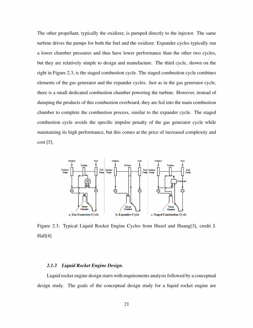
The other propellant, typically the oxidizer, is pumped directly to the injector. The same

turbine drives the pumps for both the fuel and the oxidizer. Expander cycles typically run

a lower chamber pressures and thus have lower performance than the other two cycles,

but they are relatively simple to design and manufacture. The third cycle, shown on the

right in Figure 2.3, is the staged combustion cycle. The staged combustion cycle combines

elements of the gas generator and the expander cycles. Just as in the gas generator cycle,

there is a small dedicated combustion chamber powering the turbine. However, instead of

dumping the products of this combustion overboard, they are fed into the main combustion

chamber to complete the combustion process, similar to the expander cycle. The staged

combustion cycle avoids the specific impulse penalty of the gas generator cycle while

maintaining its high performance, but this comes at the price of increased complexity and

cost [5].

Figure 2.3: Typical Liquid Rocket Engine Cycles from Huzel and Huang[3], credit J.

Hall[4]

2.1.3 Liquid Rocket Engine Design.

Liquid rocket engine design starts with requirements analysis followed by a conceptual

design study. The goals of the conceptual design study for a liquid rocket engine are

21

to determine the rocket’s layout and dimensions, estimate its weight, and calculate its

expected performance generally in terms of thrust and specific impulse. As is common

in engineering design, the design process for liquid rocket engines is an iterative one,

as can be seen in Figure 2.4. The inputs to the design process are typically generated

during a vehicle’s mission analysis. Rocket engine design inputs cover both requirements

and constraints. The requirements generally include the thrust, specific impulse, ∆v per

mission segment, the engine’s lifetime, and the “-ilities” such as maintainability, reliability,

and manufacturability. The constraints generally include cost, risk, geometric envelope,

and development schedule [5].

Figure 2.4: Liquid Rocket Engine Design Process

Once the requirements have been specified, the design process begins with an initial

estimate of the size and mass of the engine based on historical data. The weight of a liquid

rocket engine correlates strongly to thrust, propellant combination, and application (for

example in space applications versus launch vehicle boosters). Space Propulsion Analysis

22

and Design provides a number of curve fits to develop initial estimates for the engine’s

mass and size based on the thrust and application [5].

After estimating the size and mass of the engine, the designer must choose the

propellants and the oxidizer-to-fuel ratio (O/F) for bi-propellants. For a given propellant

combination, expansion ratio, and engine cycle a specific oxidizer-to-fuel ratio produces a

maximum specific impulse. This ratio produces the optimal energy release and exhaust

molecular weight from the combustion reaction. For liquid hydrogen/liquid oxygen

engines, the optimal oxidizer-to-fuel ratio is between 3.5 and 6.0 [24] [5].

The next steps in the design process are to choose the engine cycle and cooling

approach. The determining factors in the choice of engine cycle are a trade off between

performance, complexity, and cost. The engine cycle has a significant impact on the

pressure levels in the chamber and feed system. For the cooling approach, the choice

again comes down to one of performance and complexity. Generally speaking, higher

performance engines will require more complex cooling approaches. It should be noted,

choosing the expander cycle dictates the use of regenerative cooling in order to drive the

cycle’s turbine [5].

The final step in the iterative phase of the design process is to determine pressures in

the chamber and the feed system. As the propellants flow from the tanks to the combustion

chamber and eventually out to the ambient environment through the nozzle, the pressure

changes. Causes of pressure changes include losses in the plumbing and the injector face,

increases from the pumps, decreases across turbines, and the change in fluid velocity from

zero in the tanks to the required velocity to deliver the necessary mass flow. During this

step, the propellant mass flow is determined from the required thrust, and the chamber

pressure and expansion ratio are varied to obtain a design which meets the required specific

impulse. The pressure losses are then accounted for working back from the chamber to

the tanks to determine the pressure in the propellant feed lines. For pump-fed cycles, the

23

required power and pressures are balanced for the turbine(s) and pump(s) from the pressure

calculations. In expander cycle engines, lower turbine pressure ratios lead to improved

T/W by decreasing the pump mass (lower pump-pressure rise leads to small pumps) or

decreasing the chamber mass (higher chamber pressures lead to smaller chambers). The

results of the analysis from this step can be plotted in pressure level plots, such as the one

in Figure 2.5 to summarize the performance of the propellant feed system [5].

Figure 2.5: Example Pressure Plot of a Gas Generator Cycle; redrawn from Humble [5]

The above steps are iterated to converge on an initial design point. Once the initial

design point has been selected, a more detailed sizing analysis can be conducted. This

sizing analysis starts with the combustion chamber. The combustion chamber should

be as small as possible while still being large enough for the combustion process to

occur. Fully accounting for the combustion process is complex, so designers rely on

empirical data when initially sizing the combustion chamber. The throat area is the first

chamber sizing parameter to be calculated from the total mass flow, characteristic exhaust

velocity, and chamber pressure using Equation (2.13) which is based on the definition of

the characteristic exit velocity (Equation (2.5)) [5].

24

At =mc∗

pc(2.13)

The throat area is then combined with the characteristic length (L∗), a design parameter

measured in units of length and defined in Equation (2.14), to determine the chamber

volume. The characteristic length relates the chamber volume to the throat area using

historical data as a guide for sizing the chamber volume. The values computed from

Equation (2.14) represent a minimum chamber volume. Shorter values for characteristic

length lead to smaller engines, however poor combustion results from engines with values

which are too short, so designers must seek a balance between engine size and combustion

quality. Historical values for characteristic length range from 31.5 in to 39.4 in depending

on the propellant(s). Liquid oxygen and liquid hydrogen engines have values between 29.9

in and 40.2 in. Assuming the chamber is a cylinder, the volume and Mach number can then

be used to determine its cross-sectional area (and in turn its diameter) from Equation (2.15)

and its length from Equation (2.16). Note, the Mach number (M) in the chamber must be

subsonic, with typical values ranging from 0.1 (conservative designs) to 0.6 (aggressive

designs) [5].

L∗ =Vc

At(2.14)

Ac =At

M

[(2

γ + 1

) (1 +

γ − 12

M2)] γ+1

2(γ−1)

(2.15)

Lc = L∗At

Ac(2.16)

The nozzle is the next component of the engine to be sized. For traditional bell nozzles,

three parameters – the throat area, the exit area, and the length – define the size of the

nozzle. The nozzle’s throat area is already determined from the chamber sizing, since it

must match the dimensions of the chamber throat. The exit area can then be calculated

25

by solving Equation (2.11) for Ae. Finally, the length can be estimated by assuming a

percentage of the length of a 15◦ conical nozzle such as the common 80% bell nozzle.

Equation (2.17) gives the length of a conical nozzle based on its throat and exit diameters

and its half angle [5].

Ln =De − Dt

2tan(α)(2.17)

After sizing the chamber and the nozzle, the engine mass can be estimated beginning

with the chamber and nozzle, and continuing with the mass of the turbopumps, and feed

lines and structural elements. The mass of the chamber and nozzle depend on the material

used to fabricate them and the cooling approach used. However, in general, the process used

to estimate the mass of the chamber and nozzle is to calculate the required wall thickness

based on the material strength and the chamber pressure in order to calculate the volume of

material needed for the chamber and nozzle. The total volume of material is then multiplied

by the density of the material(s) to complete the mass estimation. The turbopumps, when

present, represent design processes of their own. For initial mass estimation, designers

can turn to empirical mass estimation relationships such as Equation (2.18). Similar mass

estimation relationships exist for the feed lines and the structural elements [5].

mtp = AτB (2.18)

τ =Preq

Nr(2.19)

2.1.4 Modeling Liquid Rocket Engines.

Computational modeling tools for rocket propulsion systems fall into two broad

categories. The first is high level tools to provide overall performance of traditional

rocket engine architectures. These tools generally assume the use of a bell nozzle, and

one of the classic rocket engine cycles such as the expander cycle, the gas generator

26

cycle, or the staged-combustion cycle. Tools in this category include SpaceWorks

Engineering’s REDTOP and Alexander Ponomarenko’s Rocket Propulsion Analysis. The

second category is engine cycle analysis tools such as Pratt and Whitney’s Rocket Engine

Transient Simulator (ROCETS) and NASA’s Numerical Propulsion System Simulation

(NPSS). These tools allow designers to model entire engine cycles, making them useful

in design scenarios involving new propulsion technologies and cycles.

2.1.4.1 REDTOP.

REDTOP is a liquid rocket engine analysis tool developed for use during conceptual

design studies. REDTOP runs on MS Windows and Mac OS X, and can be used from the

command line, the included graphical user interface, MS Excel, and Phoenix Integration’s

ModelCenter (through an included Analysis Server fileWrapper). REDTOP comes in

standard and lite versions, with the standard version offering more detailed analyses.

Both versions use a Gibb’s free energy combustion analysis for both included and custom

user propellants. Analyses in REDTOP include both ideal performance and real world

performance based on estimated efficiencies. REDTOP automatically provides suggested

efficiencies for the selected engine cycle and propellants, the chamber and the injector, and

the nozzle [29].

Users can model both existing engines and new engines in REDTOP. To model

existing engines, users generally specify the required mass flow of the engine being

modeled. REDTOP will return the predicted thrust, and the nozzle and exit areas. To model

new engines, users specify either required thrust and ambient conditions, the required throat

area, or the required exit area. When the required thrust is specified, REDTOP returns the

mass flow rate, and the throat and exit areas necessary to achieve the specified thrust. This

is the usual method when using REDTOP as part of a vehicle design study. REDTOP can

also return the thrust for throttle settings below 100%. After specifying one of the analysis

objectives above, users then specify the propellants, the mixture ratio, the desired chamber

27

pressure, nozzle parameters, and the cycle type. Results for REDTOP analyses include

the engine performance, the over all engine areas, and weight prediction based on both the

summation of estimated component weights and a power-to-weight ratio. In addition to the

performance and sizing analyses, REDTOP can also perform a flow separation analysis on

the nozzle, and a gimbal range check for engine clusters [29].

2.1.4.2 Rocket Propulsion Analysis.

Rocket Propulsion Analysis (RPA) is a rocket engine analysis program which runs on

MS Windows, Mac OS X, and Linux. The developer provides a free lite version, and a

standard paid version. RPA’s strengths are its flexibility in propellant options, including a

wide range of built in propellants, plus support for both custom user defined propellants

and importing CEA2 and PROPEP propellant definitions. Unlike REDTOP, RPA does not

allow the user to specify a particular engine cycle. RPA uses a simpler approach of having

the user define the chamber pressure, nozzle parameters, and propellant selections. The

user must use the RPA results in another analysis to account for the effects of the engine

cycle and the chamber design. RPA’s calculations are indicative of actual performance for

pressure fed and staged-combustion rocket engines [30].

Setting up an analysis in RPA involves three basic steps. The user begins by

defining the overall problem. In the lite version the problem definition is simply the

chamber pressure. In the standard version, the user also selects a design objective, for

example solving for a nominal thrust level at a specified ambient pressure. The second

step is to specify the propellant(s) and the mixture ratio. Note, RPA supports mono-

propellant, bi-propellant, and tri-propellant engine designs. The final step is to define

the nozzle parameters such as the exit pressure or the expansion ratio. RPA returns

internal combustion analysis at the injector, throat, and the exit plane. RPA also returns

engine performance values, both ideal and with losses, over a range of altitudes. The key

engine performance values RPA reports are the vacuum and sea level specific impulse, the

28

characteristic velocity and the thrust coefficient (cF) [30]. The engine’s actual thrust can

be calculated from the thrust coefficient from Equation (2.20) if a throat area has been

determined [24]. The standard version offers two other features over the lite version: a

JavaScript Application Programming Interface to facilitate automated analyses and trade

studies, and a chamber and nozzle geometry design and export tool [30].

F = cF At pc (2.20)

2.1.4.3 Numerical Propulsion System Simulation.

NPSS is a computer simulation tool for modeling aircraft and rocket engines. Engine

simulations built in NPSS provide higher fidelity results than engine cycle studies. NPSS

has been developed by the NASA Glenn Research Center, with assistance from the

aerospace propulsion industry. Models built in NPSS consist of a series of interconnected

software objects representing the components of the engine under consideration. The object

connections are made using NPSS Application Programming Interfaces, called “ports”,

modeling fluid flows, mechanical connections, and thermal flows. A built-in solver in

NPSS can then be used to drive the model design variables to balance the fluid flows,

mechanical power, and thermal flows in the model and converge on a design point [31].

NPSS models have four classes of variables: the dependent variables the NPSS solver

will ensure equal specified values, the independent variables the NPSS solver is free to

adjust as necessary to converge the design, component inputs read by the NPSS solver but

not altered by it, and component outputs calculated by the NPSS solver, but not driven

toward a particular value. Taken together, the NPSS dependent variables and component

inputs form the set of user specified design choices or design variables. The NPSS

independent variables and component outputs form the set of user specified responses or

response variables [31].

29

As part of the development of NPSS, NASA worked with members of the propulsion

industry to verify and validate NPSS. This effort covered both air breathing and rocket

engine modeling. Members of the NPSS development team modeled a number of engines

and compared the NPSS outputs to the actual performance of the engines in question.

Tests of the rocket capabilities in NPSS included modeling the RL10, an expander cycle

liquid hydrogen/liquid oxygen upper stage engine. NPSS performed well in these tests,

demonstrating its utility in modeling engine cycles [31, 32].

2.1.4.4 Rocket Engine Transient Simulator.

ROCETS is a modular rocket propulsion analysis tool developed by Pratt and Whitney

for NASA. ROCETS can perform both steady-state analyses to model full power operation

and transient analyses to model engine start up or shut down. Its modular design is

built around connecting rocket engine components and reusable engine models. ROCETS

supports both built-in components, such as pumps, turbines, and dynamic volumes, and

custom user components. Engine models in ROCETS are defined in a formatted text

file which is used to generate a FORTRAN program. The reusable engine models allow

designers to run multiple analysis scenarios including parametric design, steady-state

analysis, transient simulations, and generation of linear models, without recreating the

underlying engine model. ROCETS has been used to model the Space Shuttle Main Engine,

the RL10 upper stage engine, and the Space Transportation Main Engine design study [33].

2.2 Government Demand for Improved Rocket Engines

This section provides an overview of US government demand for improved rocket

engines starting with the current US government launch vehicles and then covering three

programs focused on the use of improved rocket engines. These demands are driven by US

reliance on satellites and the continued need to effectively and affordably launch them.

30

2.2.1 Current Launch Vehicles.

The US government relies on satellites for surveillance, navigation, communication,

and meteorology. Currently, the US uses the two launch vehicles from the Evolved

Expendable Launch Vehicle (EELV) program, the Delta IV and Atlas V, to deliver many of

its satellites to orbit. Both use variants of the RL10 to power their upper stages [17, 34].

The Delta IV is a family of medium-weight and heavy-weight launch vehicles. The

Delta IV Medium first stage uses a single Common Booster Core. The Delta IV Heavy

first stage uses three Common Booster Cores. The Delta IV family of launch vehicles has

two upper stage variants: the 4 m upper stage (Figure 2.6) and the 5.2 m upper stage. Both

upper stages are powered by a single RL10B-2. The RL10B-2 delivers 24,750 lbf vacuum

thrust and uses an extension nozzle to achieve a vacuum specific impulse of 465.5 s. The

RL10B-2 has a thrust-to-weight ratio of 37.3 [11, 34].

Figure 2.6: Delta IV Upper Stage, credit NASA KSC [6]

The Atlas V is the latest launch vehicle in the Atlas family going back to 1959. Current

Atlas launch vehicles come in two variants offering different sized payload fairings. The

31

Atlas V 400 series has a 4 m diameter fairing and the Atlas V 500 series has a 5.4 m

fairing. Both variants use the same Centaur upper stage (Figure 2.7), powered by one or

two RL10A-4-2 rocket engines. The RL10A-4-2 generates 22,300 lbf vacuum thrust with

vacuum specific impulse of 451.0 s and thrust-to-weight ratio of 60.3 [34, 35].

Figure 2.7: Centaur Upper Stage, credit NASA KSC [7]

2.2.2 US Air Force Next Generation Launch Programs.

The thrust-to-weight ratio of high thrust liquid rocket engines follows a decades long

trend documented by B. McHugh in 1995 [23]. McHugh’s research covers bi-propellant

liquid rocket engines producing thrust between 60,000 N (13,500 lbf) and 8,000,000 N

32

(1,800,000 lbf). He based his results on data from fourteen rocket engines developed

over 40 years, which included one expander cycle engine, and a mix of gas generator and

staged combustion cycle engines. One of McHugh’s findings was the clustering of thrust-

to-weight ratios for rocket engines, as opposed to the thrust-to-weight ratios of the launch

vehicles, based on their propellants. He found liquid hydrogen/liquid oxygen engines have

vacuum thrust-to-mass ratios (T/M) between 0.4 and 0.6 kN/kg, and RP-1/liquid oxygen

engines have vacuum thrust-to-mass ratio between 0.7 and 1.0 kN/kg. Multiplying these

values by 1000 N/kN and dividing by 9.81 m/s2 converts McHugh’s values to traditional

vacuum thrust-to-weight ratios, shown in Table 2.1 [23].

Table 2.1: Thrust-to-Weight Range Based on Propellants

LH2/LOX RP-1/LOX

T/M (kN/kg) 0.4 - 0.6 0.7 - 1.0

T/W 41 - 61 71 - 102

Since 1996, the Department of Defense, NASA, and the aerospace propulsion industry

have been working to double U.S. rocket propulsion capability when compared with 1993

rocket propulsion capability including thrust-to-weight ratios. Two major programs have

been started to meet this goal. The first is the Integrated High-Payoff Rocket Propulsion

Technology program (IHPRPT). Scheduled to end in 2010 with an extension to 2012,

IHPRPT was divided into propulsion categories (boost, orbit transfer, and spacecraft

propulsion) and phases. Research into upper stage rocket engines continues in the Phase

III orbit transfer efforts. The goals for the Phase III orbit transfer research are to improve

vacuum specific impulse and thrust-to-weight ratio, and to reduce the costs and failure

rates of launch vehicle upper stages. The anticipated benefits of meeting these goals are to

33

increase expendable launch vehicle payload mass by 22% and reduce their launch costs by

33% [19].

The second program is the U.S. Air Force’s Next Generation Engine (NGE) which

seeks to replace the RL10 on both the Delta IV and the Atlas V by 2017. Since the NGE

is intended to replace the RL10, the Air Force is requiring the NGE to be compatible

with the Delta IV and the Atlas V. The NGE must use the same propellant combination as

the RL10, liquid hydrogen/liquid oxygen, and it must be able to integrate on both launch

vehicles. Performance requirements include vacuum thrust in the range of 25,000 lbf to

35,000 lbf, a vacuum specific impulse of at least 465 s, and a life expectancy of at least

3000 s. Size constraints for the NGE are a maximum length (gimbal to nozzle exit) of 90

in, and a maximum exit diameter of 73 in [18].

The RL10B-2 falls just outside of these requirements. Its 24,750 lbf vacuum thrust is

just under the NGE minimum thrust and its high-expansion ratio nozzle has a diameter of

84.5 in exceeding the NGE constraint by nearly 16%. It is worth noting, the RL10B-2’s use

of an extendable nozzle gives an engine length of 86.5 in when stowed, meeting the NGE

constraint despite its high expansion ratio [11].

2.2.3 NASA’s Space Launch System.

NASA has its own upper stage engine requirements centered on the Space Launch

System (SLS). The SLS is a shuttle derived super-heavy lift human-rated launch system

which is still in the design phase. As a human-rated launch vehicle, work on the SLS is

closely coordinated with the Orion crew capsule program. Its super-heavy lift capacity,

between 70 metric tons and 130 metric tons to low-Earth orbit, is crucial to its role as a

launcher for missions beyond Earth orbit [22].

Four upper stage configurations are being considered for the SLS, with two

configurations being relevant to this research. The first design is an upper stage powered

by four RL10 engines, using the RL10B-2 version or a similar design. This configuration

34

is shown in Figure 2.8. The quoted performance for the RL10s used in this design is a

vacuum thrust of 24,750 lbf and a vacuum specific impulse of 462.5 s. The four RL10

engines together give a total vacuum thrust of 99,000 lbf and have a total weight of 2656

lbf for a thrust-to-weight ratio of 37.3 [8, 36]. Table 2.2 summarizes the four RL-10 cluster

performance and dimensions.

Figure 2.8: SLS Upper Stage with Four RL10 Engines, credit The Boeing Corporation [8]

35

Table 2.2: Key Performance Parameters for the SLS RL10 Rocket Engine Cluster [8, 11]

Parameter Value

Vacuum Specific Impulse (s) 462.5

Vacuum Thrust (lbf) 99,000

Thrust-to-Weight Ratio 37.3

Outer Radius (in) 108.0

Stowed Length (in) 86.5

The second of these designs is an upper stage powered by a single J-2X engine, shown

in Figure 2.9. The J-2X is the successor to the LOX/LH2 engine which powered the Saturn

V’s upper stage. Like the J-2, the J-2X is powered by a gas generator cycle. The J-2X is

being designed to have a vacuum thrust of 294,000 lbf, a vacuum specific impulse of 448

s, and a weight of 5,450 lbf giving it a thrust-to-weight ratio of 55 [8, 12, 37]. Table 2.3

summarizes the J-2X performance and dimensions.

Table 2.3: Key Performance Parameters for the J-2X Rocket Engine [12, 13]

Parameter Value





Length (in) 180.0

36

Figure 2.9: SLS Upper Stage with Single J-2X Engine, credit The Boeing Corporation [8]

2.2.4 US Air Force Space Plane Program.

In addition to its research into next generation expendable launch technologies, the

US Air Force has also renewed its interest in reusable space planes. The result is the

X-37 Space Maneuvering Vehicle, a test platform for advanced spaceflight hardware and

37

technologies including automated approach and landing, light weight and high performance

thermal protection systems, and hot structure control surfaces. Development of the X-37 is

a joint project including contributions from the US Air Force, various NASA centers, and

private industry. The X-37 has been developed in two phases, each targeting a separate

technology demonstration vehicle. The first phase, using the Approach and Landing

Vehicle (ALTV), focused on aerodynamic testing and proving the function of the automated

approach and landing system.

The second phase, which is ongoing, uses the Orbital Test Vehicle (OTV) to test the

on orbit and reentry technologies including the thermal protection systems and the hot

structure control surfaces [20]. Two X-37 OTVs have been built and flown to date. The

first vehicle, OTV-1, completed its mission of 225 days on December 3, 2010. The second

vehicle, OTV-2, was first launched on March 5, 2011.[38] Figure 2.10 shows the OTV in

its launch configuration aboard an Atlas V [9].

The X-37 OTV uses an AR2-3 hydrogen-peroxide/kerosene engine for on orbit

maneuvers [21]. Figure 2.11 shows a view of the AR2-3 engine on the OTV after one

of its missions. The AR2-3 has a long history with the US Air Force. It was developed by

the Rocketdyne corporation between 1955 and 1969. The original mission of the AR2-3

engine was to augment jet fighter propulsion systems to give the aircraft increased speed

and allow them to reach increased altitudes. The AR2-3 programs were quite successful,

accumulating over a dozen hours of operation and allowing aircraft to reach altitudes of

121,000 ft [39].

The AR2-3 generates 6600 lbf of vacuum thrust which can be throttled down to 3300

lbf. Its vacuum specific impulse of 246 s is much lower than the other engines mentioned

in this chapter. The AR2-3 is powered by a gas generator cycle using the mono-propellant

reaction of the hydrogen-peroxide oxidizer with a catalyst to drive the turbine. Table 2.4

summarizes the AR2-3 performance and dimensions [14].

38

Figure 2.10: X-37 Orbital Test Vehicle, credit US Air Force [9]

Table 2.4: Key Performance Parameters for the AR2-3 Rocket Engine [14]

Parameter Value


Vacuum Thrust (lbf) 6600



Length (in) 32.0

39

Figure 2.11: Rear View of X-37 including the AR2-3 Engine, credit US Air Force [10]

2.3 The Dual-Expander Aerospike Nozzle Upper Stage Engine

The focus of this research is the design and evaluation of a new liquid hydrogen/liquid

oxygen upper stage rocket engine being studied at the Air Force Institute of Technology.

This new engine is the Dual-Expander Aerospike Nozzle (DEAN). The DEAN is named

after its two key design choices, the use of two separate expander cycles and an aerospike

nozzle. This section covers the DEAN’s architecture, research history pertaining to its key

design choices, and AFIT’s research and design work on the DEAN.

2.3.1 DEAN Architecture.

The DEAN architecture, shown in Figure 2.12, uses two novel design choices. The

first is the use of separate expander cycles for the fuel and the oxidizer. In a traditional

expander cycle, the fuel is pumped through a cooling jacket for the chamber and nozzle.

The heat picked up by the fuel from cooling the chamber and nozzle is then used to drive

the turbine that runs both the fuel and oxidizer pumps before the fuel is introduced into the

chamber [5]. In the DEAN, the fuel and oxidizer each drive their own turbines to power

their own pumps.



40



compensation, making them more efficient over a range of altitudes. Similar bell nozzles

operate most efficiently at their specific design altitude [24]. In the DEAN, the use of an

aerospike nozzle provides a second, physically separate cooling loop from the chamber for

use in the fuel expander cycle.

Figure 2.12: DEAN Architecture, credit J. Hall (unpublished)

The DEAN’s unique architecture offers a number of advantages. The second cooling

loop increases the surface area inside the chamber, transferring greater energy to the

propellants and in turn providing more power to the turbines, providing for correspondingly

increased power to the pumps and in turn increased chamber pressure. The increased

chamber pressure leads to engine performance improvements when compared to traditional

41

expander cycle engines such as the RL10. This improved performance leads to smaller

engines for similar levels of thrust and specific impulse in terms of both weight and

physical dimensions. The separate expander cycles also ensure the fuel and oxidizer

remain physically separated until entering the combustion chamber, eliminating one of

the more catastrophic failure modes in traditional expander cycles, namely failure of an

inter-propellant-seal. The DEAN architecture is also a forerunner to a similar boost stage

architecture, where the aerospike nozzle’s global performance could result in even greater

performance gains [2, 25–27].

The DEAN architecture is not without its challenges, though. The LOX cycle requires

a turbine material able to withstand an oxygen environment. Material studies at AFIT have

shown Inconel 718 provides both satisfactory oxygen resistance and suitable mechanical

performance for use in both the pump and the turbine in the LOX cycle [26, 27]. Also,

the expansion ratio of aerospike nozzles is limited to the ratio of the area of the chamber

at the throat to the throat area [24]. Due to this limit, aerospike nozzles generally need

larger chamber diameters to reach useful expansion ratios, potentially limiting the range

of engines which offer improved thrust-to-weight ratios while also delivering the required

specific impulse.

2.3.2 Research History of Core Technologies.

This section covers the research history of the two key features of the DEAN

architecture. First it covers dual-expander research, both dual fuel based cycles and the

cycles using separate expander cycles for the two propellants like the DEAN. Second, it

reviews the history and testing of aerospike nozzles from the 1950s to he present.

2.3.2.1 Dual-Expander Cycles.

Two separate meanings of dual-expander cycle show up in the literature. The first,

and more prevalent meaning is also called the Dual-Fuel/Dual-Expander cycle (DF/DX).

Research into the DF/DX engine cycle was conducted in the late 1980s and early 1990s

42

to develop an engine for use in Single-Stage-to-Orbit launch vehicles. The DF/DX cycle

utilizes a dense hydrocarbon fuel, such as RP-1, and liquid hydrogen with liquid oxygen

in a dual chamber/dual nozzle configuration. The pervasive dual nature of the engine cycle

allows the engine to run with a mix of fuels for low altitude operations during launch,

making use of the higher density fuel early in the the flight, and transitioning to pure liquid

hydrogen at higher altitudes and in orbit for its high specific impulse. Research showed

engines utilizing this cycle to be significantly smaller and lighter than comparable engines

utilizing traditional cycles. It should be noted, the DF/DX cycle utilizes preburners to drive

its turbines, and is not related to the traditional expander cycle [40–43].

The second, and less prevalent meaning of dual-expander in the literature is that of

the DEAN, namely the operation of separate expander cycles for the fuel and oxidizer.

Research into this cycle shows chamber pressures as high as 2000 - 3000 psia are possible

with the dual-expander cycle, which are significantly higher than traditional expander

cycles. Aerojet TechSystems used cooling channels in both the chamber and the nozzle

to drive the fuel cycle and cooling channels in chamber to drive the oxidizer cycle in their

proposed dual-expander cycle engine. Aeroject’s proposed engine had a vacuum thrust

of 3750 lbf, and would be grouped into a cluster of four engines to meet the 15,000 lbf

vacuum thrust requirement of the Orbital Transfer Vehicle. As part of the research into

this engine, Aerojet built and tested a complete oxygen turbine/pump assembly built out

of Monel, a nickel/copper alloy used in high performance aerospace applications. The

successful testing of this turbine/pump assembly conducted at Aerojet demonstrated the

feasibility of building and operating a liquid oxygen expander cycle [44].

2.3.2.2 Aerospike Nozzles.

Rocketdyne is credited with developing the aerospike nozzle concept in the 1950s

[45, 46], and while the aerospike nozzle has not been used in an operational propulsion

system, there are numerous publications in the literature covering the performance, design,

43

and testing of aerospike nozzles. Research into the performance of aerospike nozzles dates

back to the 1950s and continues to this day. NASA research has included investigations

into the effect of design parameters including base bleed, nozzle area ratio, and plug length

on performance. Results from this research indicate a small base bleed (no more than

1% of total mass flow) can offer significant performance gains [47]. Research at the

California State University at Long Beach (CSULB) is investigating the affect of nozzle

truncation on aerospike performance. The CSULB researchers developed Computational

Fluid Dynamics (CFD) models of full length and 20% truncated aerospike nozzles. Their

findings indicate there is a negligible difference (0.2%) in thrust between the full length and

20% truncated aerospike nozzles, which would favor the lighter truncated design. Note, the

CSULB research did not address the specific impulse of the two nozzles [46].

Much of the research into the design of aerospike nozzles has focused on means

of determining the nozzle contour. As early as 1964, Gianfranco Angelino proposed

an approximation method to calculate the contour of two-dimensional and axisymmetric

aerospike nozzles. His approximation is based on an assumption of linear characteristic

lines with constant properties and a choked (or sonic) throat [48]. Modern computer codes,

such as Software Engineering Associates’ Two-Dimensional Kinetics (TDK) implement

the Method of Characteristics (MoC) to calculate the contour of aerospike nozzles. TDK

can also calculate the nozzle’s performance in the same analysis run, making it a powerful

tool in aerospike modeling [49]. Research in 2001 at the Beijing University of Aeronautics

and Astronautics looked at designing aerospike nozzle contours by optimizing the total

impulse over the entire proposed trajectory. Their findings indicate this approach not only

delivers improved average performance, but also improved performance over bell nozzles

at low and high altitudes [50] In recent years, California Polytechnic State University has

developed its own software to determine the contour of a minimum length aerospike nozzle.

Their software requires three parameters: the pressure ratio between the chamber and

44

ambient conditions (or Nozzle Pressure Ratio), the ratio of specific heats, and the ambient

pressure. Unlike some other techniques, this software does not require the specification of

the upstream geometry to calculate the aerospike nozzle’s contour [51].

Research tests of aerospike nozzles have led to the development and testing of four

aerospike engines, two of which have been flown on experimental sounding rockets. The

earliest aerospike engine, the liquid hydrogen/liquid oxygen J-2T (Figure 2.13(a)), was

developed by Pratt and Whitney Rocketdyne in the 1960s. As the name implies, the J-2T

was a modified Saturn V J-2 upper stage engine. The goal of this program was to compare

the performance of the aerospike nozzle with the existing bell nozzle on the production J-2

engine. The J-2T was not flown on any missions, but it was fired on a Pratt and Whitney

Rocketdyne test stand [52]. The next aerospike engine to be built was developed in the

1990s in support of NASA’s X-33 single-stage-to-orbit launch vehicle. As with the J-2T, the

X-33’s XRS-2200 linear aerospike engine (Figure 2.13(b)) ran on liquid hydrogen/liquid

oxygen, and was only operated on a test stand [53].

Two experimental sounding rockets have been used for flight testing of aerospike

nozzles. One, the Optimal 168, was a solid fueled rocket developed as part of a joint

research program between NASA, the U.S. Air Force, Blacksky Corporation, and Cesaroni

Technology/Cesaroni Aerospace. This research effort included developing two sister

sounding rockets, one with a conical nozzle and one with an aerospike nozzle to compare

the performance of the two nozzles. Flight tests of the Optimal 168 provided the first set of

transonic flight data for aerospike rockets, but did not provide the anticipated comparison

between the two nozzles as the chamber pressures and thrusts for the aerospike nozzle

were lower than predicted. The authors concluded this discrepancy was caused by a larger

than designed throat area in the aerospike nozzle [54]. The second sounding rocket to test

aerospike nozzles, Garvey Spacecraft Corporation’s (GSC) Prospector-2B (Figure 2.13(c)),

included the first liquid propellant aerospike engine to be flown. The Prospector-2B was

45

powered by a pressure fed ethanol/liquid oxygen ablative cooled engine, and produced 1000

lbf of thrust at sea level. GSC flew the Prospector-2B twice to demonstrate the feasibility of

their design. GSC continued their development program by working on a high-expansion

ratio aerospike engine for use in a Nanosat Launch Vehicle (NLV) [55, 56].

(a) J2-T Test Fire, credit Boe-

ing/Rocketdyne [57]

(b) XRS-2200 Test Fire, credit

NASA MSFC [58]

(c) Prospector 2 Aerospike En-

gine, credit Kim Garvey [59]

Figure 2.13: Example Aerospike Engines

2.3.3 DEAN Research History.

The research presented here builds on four generations of previous DEAN models.

All four generations use NPSS to implement their cycle model. Three of the four

previous DEAN models extend the cycle model by embedding it in a system level engine

model built in Phoenix Integration’s ModelCenter. ModelCenter is a multidisciplinary

modeling environment used to study the trade space of a design and optimize that design.

ModelCenter can combine analyses developed in a variety of tools including MATLAB,

Mathcad, Excel, and command line executables into a single system level model [60]. The

system level DEAN simulation automates a parameterized version of the cycle model and

connects it to additional analyses to estimate the DEAN’s weight and geometry in order to

compute the DEAN’s physical dimensions and thrust-to-weight ratio.

46

The first generation research focused on developing the initial cycle model of the

DEAN for a single design point. The second generation research implemented parametric

modeling of the DEAN by refactoring the cycle model and integrating it into the first

system level model. The third generation research extended the system model to include

additional calculations such as structural sizing, nozzle contour, and engine weight. Finally,

a parallel research effort was conducted to determine the feasibility of developing a DEAN

fueled with methane in place of liquid hydrogen. The following subsections summarize the

methodology and results of these research efforts.

2.3.3.1 First Generation DEAN.

From 2007 to 2008, AFIT researched the DEAN architecture in a series of three

projects. The initial performance goals for the DEAN were a vacuum thrust of 50,000 lbf,

a vacuum specific impulse of 464 s, and a thrust-to-weight ratio of 106.5. The first project,

conducted by D. Martin, demonstrated the feasibility of the DEAN’s over all engine cycle

by developing the initial cycle model. This first cycle model was hard coded for a single

design. The remaining two projects, conducted by A. Arguello and W. Strain, verified

the performance of the individual expander cycles for Martin’s design using Pumpal and

RITAL, industry standard pump and turbine design software respectively [2, 25, 26].

Martin focused his work on the design and modeling of the chamber, cooling jackets,

and nozzle. His design process began by making initial estimates for three key properties

of the DEAN: the oxidizer-to-fuel ratio (7.0), the expansion ratio (125), and the chamber

pressure (1740 psia). Martin selected these initial values to maximize the vacuum specific

impulse, using the RL10 as a guide. Based on these values, Martin then calculated an

estimated mass flow and sized the chamber, nozzle, and cooling channels. The inputs

Martin chose for the chamber were its radius, length, and the contour of the chamber’s

outer and inner walls. The outputs for the chamber design were the chamber pressure and

temperature. The inputs Martin chose for the nozzle were the throat area, the expansion

47

ratio, and its length. The outputs for the nozzle were the vacuum thrust and vacuum specific

impulse [2].

For the cooling channels, Martin elected to use milled channels over tubular

channels. His research indicated the milled channels offered both superior performance

and manufacturability. The aspect ratio of the cooling channels was not constant along

the length of the engine. Instead, the aspect ratio was varied according to cooling priority.

Near the throat, the aspect ratio is relatively low to provide maximum heat transfer, while

the aspect ratio is higher toward the end of the cooling channels to keep the flow subsonic.

The outputs for the cooling channels were the heat flow and the fluid Mach number [2].

Arguello and Strain studied the DEAN’s two expander cycles by modeling the

turbopumps in Pumpal/RITAL. These turbopump modules agreed well with Martin’s cycle

model. For example, the liquid hydrogen pump module showed the required power of the

first pump is 2523 HP (less than 1% difference from the value calculated in the cycle model)

and the required power of the second pump is 1079 HP (approximately 3% difference from

the cycle model). Further, the liquid hydrogen pump’s pressure exiting the second pump

stage is 4050 psia versus 4000 psia in the cycle model (approximately 1% difference) [25].

The liquid oxygen pump module showed similar agreement. For example, the results for the

liquid oxygen pump showed the required power is 2215 HP (approximately 12% difference

from the cycle model) and the pressure generated by the liquid oxygen pump is 4600 psia

versus 4500 psia in the cycle model (approximately 2% difference) [26].

Martin’s final design, shown in Figure 2.15(a), exceeded the design goals. The DEAN

model produced a vacuum thrust of over 57,000 lbf (+14%) and a vacuum specific impulse

of more than 472 s (+1.8%). The predicted thrust-to-weight ratio was 119, beating the

design goal by almost 12%, and engine length was 38 in, 61% shorter than the RL10B-2

[2]. Further, the results of the combined efforts of Martin, Arguello, and Strain confirmed

48

the feasibility of the DEAN and verified the expander cycles in Martin’s NPSS model of

the DEAN.

2.3.3.2 Second Generation DEAN.

The second generation research focused on the development of the first system level

DEAN model, shown in Figure 2.14. The DEAN model employed parametric modeling

techniques, modified design variables, and a simplified nozzle geometry. The pressure

ratios of the pumps were replaced as inputs with the total mass flow and the oxidizer-to-

fuel ratio. The DEAN geometry was determined from the chamber’s inner and outer radii

and the chamber length parametrization. The assumption of an expansion ratio of 125 was

maintained in this model [27].

Figure 2.14: Second Generation DEAN Model

The new DEAN model was then used to run parametric studies over the chamber

geometry and propellant flow using the chamber length and radii, total mass flow, and

oxidizer-to-fuel ratio as design variables. While parametric studies over total mass flow and

49

the oxidizer-to-fuel ratio yielded a large number of valid designs, parametric studies over

chamber geometry were less successful. Only studies over the chamber length produced

significant numbers of valid designs. Attempting to vary the chamber’s radii resulted in

computational errors in the cycle model. In total, the completed parametric studies yielded

more than one hundred new designs in the DEAN trade space, further demonstrating the

feasibility of the DEAN architecture [27].

The results of the parametric studies were then used to scale down the DEAN design to

more closely match the original design goals. The resulting design had a vacuum thrust of

50,900 lbf and a vacuum specific impulse of 489 s, while being 25% shorter in total length

and reducing the size of the turbomachinery by reducing the total mass flow. Figure 2.15

compares the original DEAN geometry with the scaled DEAN [27].

This research both expanded the DEAN trade space and demonstrated the power

of combining engine cycle models with parametric modeling in the development of new

liquid rocket engines. The expanded trade space resulted in a significantly improved

design for the DEAN. Further, finding such an improved design using basic parametric

modeling capabilities showcased the power of parametric modeling in rocket engine design

[27]. Chapter 3 covers the research in more detail, and also appears as an article in the

March/April 2011 volume of the AIAA Journal of Spacecraft and Rockets [27].

2.3.3.3 Third Generation DEAN.

Hall built upon the initial system level model in the second generation DEAN to

perform a detailed estimation of the DEAN’s performance, weight, and geometry. Hall

continued to work towards the original design goals of 50,000 lbf vacuum thrust, 464

s vacuum specific impulse, and a thrust-to-weight ratio of 106.5. The third generation

DEAN includes a number of new analysis codes including a custom implementation of the

aerospike’s geometry, NASA’s Chemical Equilibrium with Applications (CEA) to estimate

50

chamber properties for analyses, executed before the cycle model, and Two Dimensional

Kinetics (TDK) to improve the model’s performance estimates [4].

Hall’s research noted the assumed expansion ratio did not match the DEAN geometry.

As discussed in Section 2.1.2, the expansion ratio of an aerospike nozzle is limited by

the area of the chamber at the throat. Additionally, the length of an aerospike nozzle

is directly related to its expansion ratio [24]. Previous DEAN research efforts simply

assumed an expansion ratio of 125 and a similarly assumed nozzle length. Hall updated the

nozzle module to calculate the expansion ratio from the outer throat radius and throat area,

significantly reducing the vacuum specific impulse. Hall ran a number of trade studies

in search of designs to improve the vacuum specific impulse result. However, the third

generation DEAN model was unstable during studies varying the chamber radii, making it

difficult to improve the expansion ratio and in turn the vacuum specific impulse [4].

Hall used the updated DEAN system level model for verification studies showing the

underlying cycle model provides reliable results. An initial survey into the component

materials to be used to construct the DEAN was necessary to estimate the thrust-to-weight

ratio of the engine for the third generation’s final design. The survey results conclude the

chamber should use silicon carbide for its cooling jacket and aluminum 7075 T6 for its

structural jacket. The aerospike nozzle would best benefit from being fabricated from a

single material, oxygen-free copper (C10100) [4].

The third generation research produced a final design with a vacuum thrust of 50,000

lbf, 430 s vacuum specific impulse, and a thrust-to-weight ratio of 142 (27 inch envelope).

This design exceeds the required thrust-to-weight ratio and delivers the required vacuum

thrust; however, it falls far short of the desired vacuum specific impulse. These results

highlight the need for a parametrization of the DEAN geometry enabling the model to

run over a wider range of expansion ratios. Additionally, exposing more turbomachinery

51

variables to the ModelCenter environment will allow for the execution of trade studies over

turbine efficiencies and shaft speeds [4].

(a) First Generation DEAN Ge-

ometry

(b) Second Generation DEAN

Geometry

(c) Third Generation DEAN Ge-

ometry

Figure 2.15: Comparison of First, Second, and Third Generation DEAN Geometry

2.3.3.4 Methane DEAN.

From 2011 to 2012, AFIT conducted a parallel line of research to explore the

feasibility of a methane powered DEAN engine. This research was carried out by M.

Moen. The focus of Moen’s work was to adapt the cycle model to utilize methane as the

fuel in place of liquid hydrogen. Adjusting for the different performance characteristics

of methane versus liquid hydrogen and changes in research goals at the US Air Force led

Moen to target a different design goal with the Methane DEAN. This new design goal was

to develop an engine with 25,000 lbf vacuum thrust, 383.0 s vacuum specific impulse, and

a thrust-to-weight ratio of 108.0. In addition to implementing the required changes to the

cycle model to support methane as a fuel, Moen also utilized a number of improvements

to the system level model developed by the author based on Hall’s recommendations from

the third generation DEAN, research demonstrating their utility and function [61].

Moen’s research resulted in a design delivering 25,000 lbf vacuum thrust with a

vacuum specific impulse of 349.3 s and a thrust-to-weight ratio of 120.7 in a 23 inch long

engine. As with previous DEAN research, the initial Methane DEAN design exceeds the

thrust-to-weight ratio requirement while falling short of the specific impulse requirement.

52

Similarly, the Methane DEAN’s physical dimensions are also much smaller than traditional

upper stage engines. Moen completed his study of the Methane DEAN by conducting a first

order comparison of stage sizes and payload capacities between the Methane DEAN and

traditional upper stages engines. As expected, he found the shortfall in specific impulse

was not completely accounted for by the excess in thrust-to-weight or the compact size of

the Methane DEAN [61].

2.4 Engineering Optimization

This section covers a number of topics concerning engineering optimization. It opens

with essential terminology used to define and discuss engineering optimization problems.

The section continues with a discussion of how optimization problems are formally defined.

Finally, the section closes with a review of optimization algorithms used in this research.

2.4.1 Optimization Terminology.

Engineering optimization is the process of finding designs with the minimum “costs”

or the maximum “benefits” subject to technical and business limitations. The formal

application of optimization to engineering problems seeks to minimize or maximize a

function describing one or more aspects of the system being designed. This function is

called the objective of the optimization problem and represents the criterion for selecting

the best design among the available designs. Optimization problems may have one

objective function or many. If the problem has only one objective function, it is said to

be a single objective problem. If the problem has more than objective, it is said to be a

multi-objective problem [62].

The parameters defining the design of a system fall into two categories. Those

parameters that can be set to fixed values during earlier stages of the design process are

called preassigned parameters. The remaining parameters are the design variables, so

called because they represent unknown values to be determined by the design process. The

objectives defined above are functions of the design variables. The design variables can

53

be recorded as a vector with each element in the vector representing an individual design

variable. The n-dimensional space defined by treating the design vector as a coordinate

vector is the design space [62].

Optimization problems can be unconstrained or constrained. Unconstrained optimiza-

tion problems do not have any constraints placed on the results of the optimization. Con-

straints are additional functions of the design variables that must satisfy various equality or

inequality conditions for the design to be feasible. Constrained optimization problems are

problems with one or more constraints [62].

For multi-objective optimization problems with convex and competing objective

functions no single design will optimize all objectives simultaneously. Instead, these

problems yield a set of “optimal” designs called the Pareto optimum solution or Pareto

front. Each Pareto design is one such that to improve one of the objectives one or more

other objectives must be lessened [62].

2.4.2 Defining Optimization Problems.

Optimization problems are defined formally using mathematical expressions of the

objective(s), design variable(s), and constraint(s) (if present). Four examples will be

discussed below: an unconstrained single objective problem, an unconstrained multi-

objective problem, a constrained single objective problem, and a constrained multi-

objective problem.

54

2.4.2.1 Unconstrained Single Objective Problem.

Equation (2.21) gives the prototype for an unconstrained single objective optimization

problem. The problem definition starts by stating to find the value for design vector X

which solves the optimization problem. The definition then defines whether to maximize

or minimize the objective function f (X) and proceeds to define the objective function

mathematically. Finally, the definition lists any bounds on the design vector if present

[62].

Find X =

x1

x2

...

xn

which minimizes

f (X) = objective definition

where

X = design vector bounds

(2.21)

55

2.4.2.2 Unconstrained Multi-Objective Problem.

Equation (2.22) gives the prototype for an unconstrained multi-objective optimization

problem. The definition is similar to the one for a single objective problem shown

in Equation (2.21). The key difference is the inclusion of multiple objective function

definitions f1(X) through fn(X). An alternative form of multi-objective problem definitions

replaces the list of objective functions with a new, single objective function constructed

as the weighted average of the individual objective functions as shown in Equation (2.23)

[62].

Find X =

x1

x2

...

xn

which minimizes

f1(X) = objective 1 definition


...

fn(X) = objective n definition

where


(2.22)

f (X) = αa f1(X) + α2 f2(X) + . . . + αn fn(X) (2.23)

56

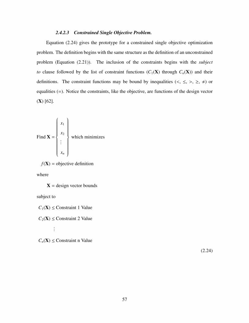
2.4.2.3 Constrained Single Objective Problem.

Equation (2.24) gives the prototype for a constrained single objective optimization

problem. The definition begins with the same structure as the definition of an unconstrained

problem (Equation (2.21)). The inclusion of the constraints begins with the subject

to clause followed by the list of constraint functions (C1(X) through Cn(X)) and their

definitions. The constraint functions may be bound by inequalities (<, ≤, >, ≥, ,) or

equalities (=). Notice the constraints, like the objective, are functions of the design vector

(X) [62].

Find X =

x1

x2

...

xn

which minimizes

f (X) = objective definition

where


subject to

C1(X) ≤ Constraint 1 Value


...

Cn(X) ≤ Constraint n Value

(2.24)

57

2.4.2.4 Constrained Multi-Objective Problem.

Equation (2.25) gives the prototype for a constrained multi-objective optimization

problem. It follows the same convention discussed above to add constraints to the multi-

objective problem definition shown in Equation (2.22) [62].

Find X =

x1

x2

...

xn

which minimizes



...

fn(X) = objective n definition

where


subject to



...

Cn(X) ≤ Constraint n Value

(2.25)

58

2.4.3 Optimization Algorithms.

Two major classes of optimization algorithms are used in this research: gradient

algorithms and genetic algorithms. Gradient optimization algorithms use the gradient of

the objective function and the constraints to guide the search for the optimal design. They

are suitable for use with single objective optimization problems using continuous design

variables. Gradient algorithms can be applied to multi-objective problems if they have

been defined using a single overall objective function like Equation (2.23). The gradient of

a function indicates the direction of steepest ascent. This property gives gradient methods

the ability to seek solutions to the optimization problem in the direction of greatest rate

of change toward the objective from the current design. However, the steepest ascent is

a local property of a function, so gradient optimization algorithms are subject to finding

local optimums. For smooth functions with no local optimums, gradient algorithms can be

efficient optimization tools as they can find optimal designs with a small number of function

evaluations. However, objective functions with local optimums which are not smooth are

generally not good candidates for use with gradient algorithms [60, 62].

Genetic optimization algorithms (GAs) apply the principles of natural selection to

engineering optimization. They are suitable for single or multi-objective optimization

problems using continuous, discreet, or a combination of continuous and discreet design

variables. The biological principles of reproduction, crossover, and mutation all play a role

in GAs. GAs operate on sets of designs called populations. Using multiple candidate

designs makes GAs less likely to become trapped in local optimums. In GAs, design

variables are represented as strings of binary variables. This representation correlates to

chromosomes in biology and facilitates the generation of subsequent generations using

“genetic” crossover between parents. The objective values are used to determine fitness

in the natural selection process implemented in GAs during the selection of the next

59

generation to intelligently and efficiently explore the trade space to find new generations

with improved values of the objective function(s) [60, 62].

2.5 Concluding Remarks

This chapter covered the engineering and technical material relevant to the research

presented in this work. The first section’s coverage of rocket powered propulsion included

essential rocket performance and design parameters used throughout the remainder of the

dissertation and reviewed traditional rocket engine cycles for comparison to the DEAN’s

architecture. The second section’s review of US space launch vehicles and demand for

improved rocket engines demonstrated the need for new rocket engine architectures like the

DEAN. The third section’s review of DEAN research history set the stage for the research

presented in the remainder of the dissertation. Lastly, the fourth section’s coverage of

engineering optimization reviewed terminology used in the final stages of this research

comparing optimized DEAN designs to traditional upper stage engines.

60

III. Parametric Study of Dual-Expander Aerospike Nozzle Upper Stage Rocket

Engine

The text of this chapter was published in the AIAA Journal of Spacecraft and Rockets,

Vol. 48, No. 2, 2011. It is unaltered from the published version except in its formatting as

required by the AFIT dissertation style guide.

3.1 Introduction

The Air Force Institute of Technology (AFIT) is studying the dual-expander aerospike

nozzle (DEAN) rocket engine architecture to significantly improve upper stage rocket

performance. The specific performance goals of this research are to provide 50,000 lbf

vacuum thrust with a vacuum Isp of 464 s. The DEAN, shown in Figure 3.1, is a liquid

hydrogen (LH2)/liquid oxygen (LOX) engine using separate expander cycles to pump the

fuel and oxidizer and an aerospike nozzle to improve efficiency.[2].

Figure 3.1: Original DEAN Geometry

61

Previous work at AFIT by Masters student David Martin focused on developing

an initial design to demonstrate the feasibility of the DEAN architecture by building

a computational model using the Numerical Propulsion System Simulation (NPSS™)

software package. That work culminated in a design exceeding the requirements.[2] This

paper outlines the current work at AFIT to optimize the DEAN’s thrust-to-weight ratio

(T/W) by expanding Martin’s model through simplifying the calculations of the DEAN

geometry and adding parametric variables to the model to support automated trade studies

in ModelCenter™. The results of those trade studies indicate the DEAN can run at the

specified performance using a lower total mass flow and a significantly shorter engine than

the previous design.

3.2 Existing NPSS DEAN Model

The original NPSS DEAN model was prepared by David Martin as part of his masters

thesis at AFIT. This model uses NPSS elements to represent the pumps, turbines, pipes,

valves, chamber, nozzle, and cooling channels to accurately model the DEAN architecture.

The results of Martin’s analysis converge to a working design, validating the DEAN

concept. The DEAN thrust, Isp, and T/W exceed both its requirements and the performance

of the upper stage single-expander cycle based RL10A-3 as can be seen in Table 3.1.

Table 3.1: Existing DEAN Design Results versus Requirements

DEAN[2] Requirement[2] Delta RL10A-3[63] Delta

Vac Thrust (lbf) 57,231 50,000 +14.5% 16,500 +247%

Vac Isp (s) 472 464 +1.7% 443 +6.5%

T/W 119 106 +12% 53 +124%

This excess in thrust performance suggests the the dual-expander cycle offers an

advantage in thrust over the single-expander cycle, and it indicates room to optimize

62

the DEAN design further. Before discussing the changes made to Martin’s model[2],

necessary to facilitate this optimization, it is useful to review the key elements of the DEAN

architecture and Martin’s model.

3.2.1 Existing DEAN Architecture.

The DEAN uses two novel design choices. The first is the use of separate expander

cycles for the fuel and the oxidizer. In a traditional expander cycle, the fuel is pumped

through a cooling jacket for the chamber and nozzle. The heat picked up by the fuel from

cooling the chamber and nozzle is then used to drive the turbine that runs both the fuel and

oxidizer pumps, before the fuel is introduced into the chamber.[5]

Figure 3.2 shows the DEAN’s two separate expander cycles. The fuel loop is on the

left. Here, the LH2 flows from the fuel tank into the first fuel pump. Half of the liquid

hydrogen then flows through a bypass, while the remainder is fed into a second fuel pump.

This flow then continues into the aerospike nozzle, where it absorbs heat while cooling the

nozzle. The heated flow then drives the fuel turbine before joining with the bypass flow and

entering the combustion chamber through the injector. On the right is the oxidizer loop. In

this loop, the LOX flows from the oxidizer tank into the single oxidizer pump. This flow

then enters the cooling jacket for the combustion chamber, where it absorbs heat while

cooling the chamber. The heated oxygen then flows toward the oxidizer turbine, with a

small amount (roughly 10%) sent around the turbine using a bypass and the remainder used

to drive the turbine. Finally, the oxygen flows are joined before entering the combustion

chamber through an injector.[2]

The two separate expander cycles present benefits and challenges. Increased chamber

pressures and in turn engine performance can be obtained by separating the power demands

between two separate turbines driven by separate working fluids. The separate expander

cycles also ensure the fuel and oxidizer remain physically separated until entering the

combustion chamber, eliminating one of the more catastrophic failure modes in traditional

63

Figure 3.2: DEAN Architecture

expander cycles, namely failure of an inter-propellant-seal.[2] However, the LOX cycle

requires a turbine material which will work well in an oxygen environment. Additional

research at AFIT showed that Inconel 718 provides both satisfactory oxygen resistance

and suitable mechanical performance for use in both the pump and the turbine in the LOX

cycle.[26]

The second novel design choice is the use of an aerospike, or plug, nozzle. Traditional

bell nozzles are optimized to perform at a single pressure or altitude. This optimization

makes them very efficient at their design point, but much less so for the remainder of the

flight. Aerospike nozzles on the other hand, due to their geometry, adapt their performance

to the current altitude. Even though aerospike nozzles perform less efficiently than bell

nozzles at the design altitude of a given bell nozzle, when considering the altitudes seen

64

by a launch vehicle, the global performance of an aerospike nozzle exceeds the global

performance of a bell nozzle, making the aerospike nozzle an attractive design for launch

vehicles. More importantly for the DEAN the use of an aerospike nozzle provides a second,

physically separate cooling loop from the chamber for use in the second expander cycle.

This second cooling loop increases the surface area inside the chamber used to drive the

turbomachinery, providing for correspondingly increased power to the pumps and increased

chamber pressure, and in turn increased engine performance.[2] The aerospike nozzle is

also shorter and lighter than a traditional bell nozzle, leading to improved packaging and

T/W. Finally, the DEAN architecture is a forerunner to similar boost stage architecture,

where the aerospike nozzle’s global performance will result in even greater gains than in

an upper stage engine.

3.2.2 NPSS Model Details.






connections are made using NPSS Application Programming Interfaces modeling fluid

flows, mechanical connections, and thermal flows called “ports”. A built-in solver in NPSS

can then be used to drive the model design variables to balance the fluid flows, mechanical

connections, and thermal flows in the model and converge on a design point.[31]

Martin’s model[2] of the DEAN engine includes elements to simulate the various

components of the engine. The combustion chamber is modeled using a RocketComb1

element which requires the chamber radius and volume. The RocketComb element also

includes ThermalOutputPorts to model heat exchange to the fuel and oxidizer. The

ThermalOutputPorts require the radius at the port’s location, the cross-sectional area

65

of the combusting flow in the chamber, and the surface area of the portion of the

chamber in contact with the combusting flow. The model calculates the heat exchange

between the chamber walls for the oxidizer expander cycle and the internal portion of

the aerospike for the fuel expander cycle. The aerospike nozzle is modeled using a

RocketNozzle element which requires the throat area and the expansion ratio and includes

more ThermalOutputPorts for use in the heat exchange between the aerospike and the fuel

expander cycle.

The fuel and oxidizer tanks are modeled using Starter elements. The plumbing

connecting the engine components to the tanks and each other is modeled using Valve04

elements which require the cross-sectional area to model the pressure drop in the plumbing

and customized CoolingVolume elements which require the cross-sectional area and fluid

volume to model the heat loss in the lines. The cooling jackets around the combustion

chamber and the aerospike nozzle are modeled using using the ThermalOutputPorts in the

chamber and nozzle and the plumbing elements connected by Wall2 elements. The pumps

are modeled using customized Pump elements which require the efficiency, pressure ratio,

and mass flow of each pump. Finally, the turbines are modeled using customized Turbine

elements which require the efficiency, pressure ratio, mass flow and the cross-sectional area

of the flow.

While the cooling jackets in the DEAN are continuous volumes, the NPSS model

represents them as a series of eight discrete stations. Figure 3.3 shows the locations of

these stations in the model. The chamber (24 inches long in Martin’s design) consists of

five equally spaced sections, with stations (represented by stars) at the mid point of each

section plus a station at the throat of the rocket. Note that the oxidizer loop (the outer

wall of the chamber) and the fuel loop (the aerospike) are represented by separate sets of

stations. The external portion of the aerospike (14 inches long in Martin’s design) has two

additional stations in the first half of the nozzle that are only in the fuel loop.

66

Figure 3.3: DEAN Geometry (dim in inches), credit D. Martin

NPSS models have four classes of variables: the dependent variables the NPSS solver

will ensure equal specified values, the independent variables the NPSS solver is free to

adjust as necessary to converge the design, component inputs read by the NPSS solver but

not altered by it, and component outputs calculated by the NPSS solver, but not driven

toward a particular value. Taken together, the NPSS dependent variables and component

inputs form the set of user specified design choices or design variables. The NPSS

independent variables and component outputs form the set of user specified responses or

response variables. In the previous model, the design variables include the user specified

dependent variables (the pressure ratios for the three pumps) and the component inputs

(for example the volume of the combustion chamber and the nozzle expansion ratio). The

response variables include the user specified independent variables (the efficiencies of the

first liquid hydrogen pump and of the liquid oxygen pump) and the component outputs

(for example the vacuum thrust and Isp). Table 3.2 summarizes the design and response

variables of the previous model.

67

Table 3.2: Existing DEAN Design Point[2]

Design Variables Response Variables

LOX Pump PR (PRp,LOX) 103 Vac Thrust (Fvac) 57,000 lbf

LH2 Pump 1 PR (PRp,LH2,1) 45 Vac Isp 472 s

LH2 Pump 2 PR (PRp,LH2,2) 2 Mass Flow (m) 121 lbm/s

LH2 Pump 2 Eff (ηp,LH2,2) 0.83 O/F 7.03

Chamber Length (lc) 24 in Chamber Pres (P0) 1739 psia

Outer Chamber Radius (rco) 6 in Chamber Temp (T0) 6586 R

Inner Chamber Radius (rci) 2 in LOX Pump Eff (ηp,LOX) 0.66

Chamber Vol (Vc) 2075 in3 LOX Pump Power 2587 HP

Throat Area (At) 15.9 in2 LH2 Pump 1 Eff (ηp,LH2,1) 0.67

Nozzle Length (ln) 14 in LH2 Pump 1 Power 2527 HP

Expansion Ratio (ε) 125 LH2 Pump 2 Power 1046 HP

LOX Turbine PR (PRt,LOX) 1.82

LOX Turbine Eff (ηt,LOX) 0.949

LOX Turbine Power 2587 HP

LH2 Turbine PR (PRt,LH2) 1.84

LH2 Turbine Eff (ηt,LH2) 0.9

LH2 Turbine Power 3573 HP

LOX Temp (TLOX,i) 179-617 R

LOX Pres (PLOX,i) 3810-4500 psia

LOX Max Mach (Mmax,LOX) 0.56

LH2 Temp (TLH2,i) 145-610 R

LH2 Pres (PLH2,i) 3670-4000 psia

LH2 Max Mach (Mmax,LH2) 0.67

68

Follow on research at AFIT focusing on designs for the LH2 and LOX pumps provides

verification for the NPSS model of the DEAN. In each design study, the respective expander

cycle is modeled using spreadsheet calculations, and Pumpal®/RITAL®. These additional

models agree well with the NPSS model. For example, the Pumpal model of the LH2

pumps shows the required power of the first pump is 2523 HP (less than 1% difference from

the NPSS value) and the required power of the second pump is 1079 HP (approximately

3% difference from the NPSS model). Further, the pressure coming out of the second pump

is 4050 psia versus 4000 psia in the NPSS model (approximately 1% difference).[25] The

LOX pump values show similar agreement. For example, the Pumpal model of the LOX

pump shows the required power is 2215 HP (approximately 12% difference from the NPSS

model) and the pressure coming out of the LOX pump is 4600 psia versus 4500 psia in the

NPSS model (approximately 2% difference).[26]

Given the importance of balancing the heat and mechanical flows in an expander cycle,

it is worth noting the performance of the turbomachinery in the existing DEAN design.

Naturally, the converged design point balances the power required by the pumps with that

provided by the turbines for each of the two expander cycles. And while the performance

of the turbomachinery may appear high when compared to RL10A which provides only

789 HP from its turbine, Pratt and Whitney built an LH2 expander cycle that produces

5900 HP as part of the an upper stage demonstrator engine.[25] This puts the LH2 cycle

well within demonstrated capability. As for the LOX cycle, research at AFIT has proposed

designs for the LOX pump and turbine which provide the required performance as a part of

this architecture.[26]

3.3 Parameteric NPSS DEAN Model

The goal of the current research at AFIT is to optimize the DEAN engine to provide the

maximum T/W while maintaining the required thrust and Isp and not violating operational

limits for the materials and working fluids. The T/W can be maximized by either increasing

69

the thrust or decreasing the weight. Since the DEAN has a fixed thrust requirement,

the optimization problem can be restated as optimizing the DEAN engine to provide the

minimum weight, subject to the previously mentioned constraints. Identifying the design

variables driving the weight of the engine and updating the model to use those variables as

the design variables enables automated searching over the design trade space for optimal

designs.

The rocket engine chamber, nozzle, and turbomachinery are the elements used

to estimate the total mass (weight) of the rocket engine during conceptual design.

The chamber and nozzle masses are driven by their geometry and material, while the

turbomachinery masses are driven by their local mass flows[5]. The model previously

captured the geometry of the DEAN as hard-coded values, tying the model to a single

design point. Additionally, the model treated the mass flows as responses. In order to use

the model to optimize the design, the NPSS model must be altered to use the chamber and

nozzle geometries and the local mass flows to the turbomachinery as design variables. This

section details the modifications made to the previous model to convert it into a parametric

model based on the design variable needs and two changes made while the NPSS model

was being modified to reflect the most recent DEAN architecture being considered.

3.3.1 Updated DEAN Architecture.

Before modifying the DEAN model to support parametric trade studies, two

architecture changes were made to the fuel expander cycle to reflect refinements in the

design. Figure 3.4 shows this updated DEAN architecture. The first change was to remove

the liquid hydrogen bypass, feeding the cooling jacket for the aerospike with the full mass

flow of the liquid hydrogen instead of only half. The second change was to require the

two fuel pumps run at the same pressure ratio, to minimize the maximum pressure ratio

required for the fuel pumps.

70

Figure 3.4: Updated DEAN Architecture

3.3.2 NPSS Model Details.

The modifications to convert the NPSS DEAN model into a parametric model

involved the chamber and nozzle geometry and the mass flows through the turbomachinery.

The system-level parameters chosen to drive the chamber and nozzle geometry are the

chamber length, the inner and outer chamber radii, and the shape of the nozzle. A

number of intermediate geometric values are determined by the shape of the nozzle. To

facilitate calculating these values, the geometry of the aerospike and cooling volumes were

simplified to linear approximations from their higher order calculations (the aerospike radii

are calculated using the method of characteristics[2]). Figure 3.5 compares the results of

these simplifications to the original geometry.

71

(a) Martin’s Geometry for the DEAN

(b) Parametric Geometry with Simplified Aerospike

Figure 3.5: Comparison of Simplified Geometry to Martin’s Original Geometry

The calculations based on these simplifications include the radius of the aerospike

at each station, Equation (3.2); the combusted flow cross-sectional area, Equation (3.3);

72

the surface area of the heat exchanges for the chamber, Equation (3.4), the aerospike

nozzle, Equation (3.5), and the cooling volumes, Equation (3.9); the cross-sectional area,

Equation (3.10) and volume of the fluid in the cooling volumes, Equation (3.11). These

values are calculated from the inner and outer radii of the chamber and the throat, the

chamber and aerospike lengths, the cooling channel half widths and half spacings, and

aspect ratios (ARs):

mplug = (rti − rci)/(0.6 ∗ lc) (3.1)

rci,i = rci + mplug ∗ xi ∗ lc (3.2)

A f low,i = π ∗ (r2co,i − r2

ci,i) (3.3)

Ahx = 2 ∗ π ∗ rco,i ∗ li (3.4)

Ahxnozz,i = π ∗ (rn,i + rn,i−1) ∗√

(rn,i + rn,i−1)2 + l2i (3.5)

n = round(π ∗ r/(winit + a)) (3.6)

wi = π ∗ r/nchannels + a (3.7)

hi = 2 ∗ wi ∗ AR (3.8)

Ahxcv,i = 2 ∗ wi ∗ n ∗ li (3.9)

73

Acv,i = 2 ∗ wi ∗ hi ∗ n (3.10)

Vcv,i = Acv,i ∗ li (3.11)

The system-level parameters chosen to drive the mass flows to the turbomachinery

are the oxidizer-to-fuel ratio (O/F) and total mass flow. These parameters also drive the

performance constraints of thrust and Isp. Equation (3.12)[5] determines the LOX mass

flow from these system-level parameters and Equation (3.13)[5] determines the LH2 mass

flow. In the original model, the O/F can only be controlled indirectly by changing the

pressure ratios of the pumps, leading to coupling effects appearing in the O/F plots. For

example, a parametric study, described in Table 3.3, varied the pressure ratio of the first

LH2 pump.

mLOX =O/F

1 + O/F∗ m (3.12)

mLH2 =1

1 + O/F∗ m (3.13)

Figure 3.6 shows the relationship between Isp and O/F for the DEAN based on this

parametric study. The peak Isp is at an O/F ratio of approximately 6. Ordinarily, this result

would be produced by a parametric study as a function of the independent variable, O/F,

implying the total mass flow was constant. Equation (3.14)[5], supports the conclusion

thrust versus O/F would follow the trend in Figure 3.6. However, Figure 3.7 shows a peak

at an O/F of 6, and then a rise toward another peak for O/F < 5.

Isp =F

mg0(3.14)

74

Table 3.3: Parametric Study over LH2 Pump 1 PR


LOX Pump PR (PRp,LOX) 103 Vac Thrust (Fvac) 49,500-60,000 lbf

LH2 Pump 1 PR (PRp,LH2,1) 30-60 Vac Isp 416-491 s

LH2 Pump 2 PR (PRp,LH2,2) 2 Mass Flow (m) 119-132 lbm/s

LH2 Pump 2 Eff (ηp,LH2,2) 0.83 O/F 4.2-11.3

Expansion Ratio (ε) 125 Chamber Pres (P0) 1500-1940 psia

Chamber Temp (T0) 5000-6660 R

Figure 3.6: Isp vs O/F, Original NPSS Model

The deviation from the describing equations rests with the assumption of constant

total mass flow. Figure 3.8 is a three dimensional plot showing thrust vs both O/F and

total mass flow. The vertical axis is the thrust, the left axis is O/F, and the back axis is the

total mass flow. The starred point is O/F equals 6. The total mass flow has a sharp turn

75

Figure 3.7: Thrust vs O/F, Original NPSS Model

as O/F decreases beyond that point, leading to the second increase in thrust as total mass

flow reaches its peak during the parametric study. To eliminate coupling effects like this

example, and an instability in the LH2 efficiencies, the user defined dependent variables

were changed to the total mass flow and an equation setting the two fuel pumps to the same

pressure ratio. The user defined independent variables were changed to the throat area, and

to the pressure ratios for all three pumps.

One final change was made to the NPSS model. In the model, the mass flow through

the oxidizer bypass was hard coded to a specific value, resulting in instabilities in the model

when the system mass flow or the O/F ratio changed. The oxidizer mass flow through the

bypass was set to be 10% of the oxidizer mass flow, and the mass flow to the oxidizer

turbine was set to 90%. These percentages were also made user configurable.

76

Figure 3.8: Thrust vs O/F and Total Mass Flow, Original NPSS Model

3.4 System-Level DEAN Model

A system-level model of the DEAN engine was built around the parametric NPSS

model in order to run automated trade studies. This system-level DEAN model was

built in ModelCenter™. ModelCenter is a multidisciplinary modeling environment used

to study the trade space of a design and optimize that design. ModelCenter can combine

analyses developed in a variety of tools including MATLAB, Mathcad, Excel, command

line executables (for example) into a single system-level model. Users can then use the

built-in trade study and visualization tools to conduct sensitivity studies to gain insight into

77

what aspects of the design are the key drivers influencing the desired results. ModelCenter

also provides a rich set of built-in optimization tools used to find values for the key drivers

optimizing the design for a given goal (such as minimizing the mass of the DEAN engine)

while ensuring constraints are not violated (such as maintaining the required thrust and Isp).

These optimization tools include a gradient optimizer, a genetic optimizer called Darwin™,

and an optimizer that utilizes surrogate models of the design space during optimization

called DesignExplorer™.[64]

Figure 3.9: System-level Model of DEAN

78

Figure 3.9 shows the system-level DEAN model in the ModelCenter interface. The

model consists of six components and two data display elements. Table 3.4 summarizes

these components.

Table 3.4: System-level DEAN Model Components

Label Name Description

1 DesignVariables a component storing the system-level design variables

2 CalculateGeometry a script component calculating the geometry parameters

for the DEAN model from the design variables

3 DEAN the parametric NPSS DEAN model imported into the

ModelCenter framework using the embedded Quick-

Wrap tool

4 Converger a direct substitution convergence loop used to converge

the guessed throat area to the calculated throat area

5 Geometry a collection of geometry primitives (surfaces of revolu-

tion and an arrow) and a script component to render the

live view of the DEAN geometry seen in (8)

6 Machs a script component that uses polynomial interpolation to

calculate the Mach numbers for the LOX and LH2 fluid

flows in the cooling volumes

7 Data Monitor a built-in ModelCenter component set to display the key

performance values from the DEAN model

8 Geometry Rendering a live preview of the DEAN geometry based on the

geometry components in (5)

79

The first four components in the DEAN system-level model are used to run the DEAN

NPSS model. The first component stores the system-level design variables. They are the

total mass flow, the O/F ratio, the inner chamber radius, the outer chamber radius, the

chamber length, and a guessed value for the throat area. The second component calculates

the nozzle radius using Equation (3.3), nozzle length based on the slope of the aerospike

nozzle, and the chamber volume using volume equations for cylinders and cones from the

design variables. The third component runs the NPSS DEAN model using the values of

the design variables and the values calculated in the CalculateGeometry component. Since

the throat area is an independent variable in the NPSS model, the NPSS solver may select

a value that does not match the guessed value. If the model chooses such a value, the

geometry values calculated from the guessed throat area (specifically the nozzle radius and

cooling volume sizes) are incorrect. The fourth component addresses this problem using a

direct substitution iteration solver. The solver directs the system-level model to be run in a

loop, substituting the NPSS calculated throat area for the guessed throat area, until the two

are the same value, closing the design.

The remaining two components in the DEAN system-level model are used for post

processing the DEAN NPSS model. The fifth component is actually four components

that are part of a ModelCenter assembly component. ModelCenter assembly components

allow model developers to group related components together to simplify the display and

management of the model. Three of the four sub-components in the geometry component

are built-in ModelCenter geometry primitives: two surfaces of revolution to render the

chamber in blue and the aerospike in red, and a twelve inch long arrow to provide a scale

for the DEAN geometry. The final sub-component is a ModelCenter script component

transforming the output from the DEAN NPSS model into geometry strings that define the

curves for the surface of revolution components.

80

The last analysis component calculates the Mach numbers for the LOX and LH2 fluid

flows in the cooling volumes. These values are critical constraints on the engine design,

as the flows cannot be allowed to reach sonic conditions. Previous constraints for these

values were a maximum Mach in the LOX flows of 0.6, and a maximum Mach in the

LH2 flows of 0.9[2]. Martin calculated the Mach numbers at each station by looking

up the speed of sound for the fluids in the Thermophysical Properties of Fluid Systems

online handbook (http://webbook.nist.gov/chemistry/fluid/)[65] from the National Institute

of Standards and Technology, based on the fluid temperatures and pressures. The Machs

component automates this process by using third order polynomials to interpolate the

speed of sound for LOX and LH2 over the temperature and pressure ranges seen in the

DEAN model. Table 3.5 summarizes the Design of Experiments (DOE) trade study used

to establish these ranges.

To create the interpolation polynomials, a set of isothermal speed-of-sound versus

pressure tables for both oxygen and hydrogen were downloaded from the Thermophysical

Properties of Fluid Systems online handbook. Table 3.6 shows the temperatures and

pressures selected for these tables. Note, the LH2 pressure range was truncated after

determining pressures above 7200 psia represented designs no longer being considered.

81

Table 3.5: Design of Experiments over O/F, Total Mass Flow, and Chamber Length


O/F 5.5-7.5 Vac Thrust (Fvac) 39,700-69,500 lbf

Mass Flow (m) 85-140 lbm/s Vac Isp 466-499 s

Chamber Length (lc) 22-30 in Chamber Pres (P0) 1798-3243 psia

Outer Chamber Radius (rco) 6 in Chamber Temp (T0) 6130-6850 R

Inner Chamber Radius (rci) 2 in Throat Area (At) 7.2-17.5 in2

Expansion Ratio (ε) 125 Nozzle Length (ln) 13.7-14.8 in

LOX Bypass (%) 90 Chamber Vol (Vc) 1810-2480 in3

LOX Pump Eff (ηp,LOX) 0.773 LOX Temps (TLOX) 162-886R

LOX Turbine Eff (ηt,LOX) 0.949 LOX Pres (pLOX) 2865-5864 psia

LH2 Pump 1 Eff (ηp,LH2,1) 0.8 LH2 Temps (TLH2) 73-634R

LH2 Pump 2 Eff (ηp,LH2,2) 0.83 LH2 Pres (pLH2) 3220-10,750 psia

LH2 Pump Eff (ηp,LH2) 0.9

82

Table 3.6: Data Ranges for Speed of Sound Tables

Fluid Temperatures (R) Pressure Range (psia),

step size = 100 psia

LOX 150, 275, 400, 525, 650, 775, 900 2800-6000

LH2 70, 165, 260, 355, 450, 545, 640 3200-7200

The speed-of-sound tables were then imported into ModelCenter for surface fitting

using the Data Import Plug-In. The interpolation polynomials were then created by running

a cubic fit to the data in ModelCenter’s Response Surface Modeling Toolkit (RSM Toolkit).

Equation (3.15) shows the polynomial generated for the speed of sound in LOX and

Equation (3.16) shows the polynomial generated for the speed of sound in LH2. Both

equations are good fits to the data as can be seen from their adjusted R2 values and a

graphical comparison to the results from the earlier design. Equation (3.15) has an adjusted

R2 value of 0.995 and Equation (3.16) has an adjusted R2 value of 0.988. Figure 3.10 shows

that Mach numbers calculated from both equations also compare favorably to results from

the earlier design of the DEAN.

aLOX,i = 6009.519 − 25.08448Ti + 0.05203138pi + 0.03725712T 2i (3.15)

+0.0004540472Ti pi − 1.669077 ∗ 10−05T 3i − 5.292126 ∗ 10−07 piT 2

i

aLH2,i = 4014.306 − 15.03106Ti + 0.7100687pi + 0.04704292T 2i (3.16)

−2.660187 ∗ 10−05 p2i − 0.0009330969Ti pi

−3.34523 ∗ 10−05T 3i + 4.862856 ∗ 10−08Ti p2

i

83

(a) LOX Mach Numbers

(b) LH2 Mach Numbers

Figure 3.10: Comparison of Fluid Mach Number Calculations

84

3.5 Results and Analysis

The analysis of the system-level DEAN model took place in two phases. First,

parametric studies were run over the chamber length, the O/F ratio, and the total mass flow

to establish the boundaries of the design trade space. The results of the parametric studies

were then used to scale the original DEAN design to more closely match the performance

goals.

3.5.1 Parametric Studies.

Table 3.7 summarizes the first parametric study of the DEAN system-level model,

which varied the O/F ratio from 5.5 to 7.5. Initial results from this trade study are

promising. The plot of Isp versus O/F in Figure 3.11 shows the peak Isp occurs at an

O/F ratio of approximately 6, just as in the previous study shown in Figure 3.6.

Figure 3.11: Isp vs O/F Ratio, System-level Model

85

Table 3.7: Parametric Study over O/F


O/F 5.5-7.5 Vac Thrust (Fvac) 56,700-60,000 lbf

Mass Flow (m) 121.25 lbm/s Vac Isp 468-495 s

Chamber Length (lc) 24 in Chamber Pres (P0) 2135-2415 psia





LOX Pump Eff (ηp,LOX) 0.773 LOX Temp (TLOX) 166-657R


LH2 Pump 1 Eff (ηp,LH2,1) 0.8 Max LOX Mach 0.40-0.41

LH2 Pump 2 Eff (ηp,LH2,2) 0.83 LH2 Temp (TLH2) 85-436R

LH2 Pump Eff (ηp,LH2) 0.9 LH2 Pres (pLH2) 4590-8340 psia

Max LH2 Mach 0.99-1.20

However, the max LH2 Mach numbers exceed the constraint value established by

Martin across the entire parametric study, as can be seen Figure 3.12. A review of the LH2

Mach numbers at all of the stations reveals the Mach numbers are within acceptable limits

for nozzle radii greater than 3.3 in. To test this conclusion, the inner chamber radius was

increased from 2.0 in to 3.3 in. However, the NPSS model could not converge because some

of the LH2 cooling volumes had become too large. Addressing this result, several cooling

volume aspect ratio calculations were adjusted until the model converged. As expected, the

maximum LH2 Mach number for this new design fell within the constraint value of 0.9.

Running the parametric study with the adjusted aspect ratios resulted in maximum LH2

86

Mach numbers between 0.81 and 0.88, enabling continued exploration of the DEAN trade

space.

Figure 3.12: Fluid Mach Numbers vs O/F Ratio, System-level Model

Figure 3.13 is the plot of Isp versus O/F ratio for the updated inner chamber radius.

The added detail in this plot shows the O/F ratio for max Isp is between 5.9 and 6.1,

higher than might be expected just based on the O/F ratio, given the RL10 upper stage

engine runs at an O/F ratio of 5.0[5]. However, while the total mass flow and most of the

geometric parameters are constant in Figure 3.13, the chamber pressure and temperature

are not. Figure 3.14 shows how chamber pressure varies with O/F and Figure 3.15 shows

how the chamber temperature varies with O/F. The chamber pressures seen in Figure 3.14

range from 2625 psia to 2875 psia. These values are considerably higher than the 640 psia

of the RL10B-2[5], or even the practical limits of a single expander cycle LOX/LH2 engine,

87

which Krach and Sutton determined to be between 1375 psia and 2300 psia[66]. This

dramatic difference in chamber pressures suggests higher chamber pressures are possible

with the dual-expander cycle of the DEAN architecture than with single expander cycles.

Figure 3.13: Detailed Isp vs O/F Ratio, System-level Model

88

Figure 3.14: Detailed Chamber Pressure vs O/F Ratio, System-level Model

Figure 3.15: Detailed Chamber Temperature vs O/F Ratio, System-level Model

89

Figure 3.16 uses a three dimensional plot with varying colors on the data points to

present all four of these variables, Isp, O/F, chamber pressure, and chamber temperature,

in a combined plot to present a unified view of their interactions. The O/F ratio is on the

left axis, the chamber pressure is on the rear axis, and Isp is on the vertical axis. Finally,

the chamber temperature is shown as the colors of the data points. This figure shows

the maximum Isp not only happens at an O/F of 6, but also at the maximum chamber

pressure, and somewhere in the middle of the chamber temperature range seen in this study.

Returning to Figure 3.15 reveals the chamber temperature for the O/F where the maximum

Isp occurs is located at a knee in the temperature curve. The trends evident in Figure 3.16

suggest the solution is simply one possible curve on a solution surface space.

Figure 3.16: Isp vs O/F Ratio, Chamber Pressure, and Chamber Temperature, System-level

Model

90

Table 3.8 summarizes the second parametric study run of DEAN system-level model,

which varied the total mass flow from 85 lbm/s to 122 lbm/s. As one would expect, thrust

is linearly related to total mass flow (Figure 3.17). A total mass flow of only 104 lbm/s is

sufficient to achieve 50,000 lbf thrust. Optimizing DEAN design near 104 lbm/s will result

in another weight savings over the original design.

Table 3.8: Parametric Study over Total Mass Flow


O/F 7 Vac Thrust (Fvac) 40,800-58,400 lbf

Mass Flow (m) 85-122 lbm/s Vac Isp 479-481 s

Chamber Length (lc) 24 in Chamber Pres (P0) 2525-2710 psia











91

Figure 3.17: Vacuum Thrust vs Total Mass Flow, System-level Model

Table 3.9 summarizes the final parametric study run on the DEAN system-level model,

considering the chamber length from 14 in to 26 in. The curve in Figure 3.18 showing

thrust versus chamber length has two transitions, one at 14.25 in and one at 22.75 in.

Noting shorter chamber lengths result in lighter engines since they require less material

drives the engine design toward the shortest chamber able to achieve the goal. This result

supports selecting a chamber not longer than 14.25 in, but further optimization is warranted.

Selecting a chamber length of 14.25 in results in a total engine length of 27.85 in. The new

length is nearly 25% shorter than the original design, and 69% shorter than the RL10B-

2[24]. This result suggests that the DEAN architecture can be packaged in a considerably

smaller volume than existing upper stage engines.

92

Table 3.9: Parametric Study over Chamber Length


O/F 7 Vac Thrust (Fvac) 57,100-58,200 lbf

Mass Flow (m) 121.25 lbm/s Vac Isp 471-480 s

Chamber Length (lc) 14-26 in Chamber Pres (P0) 950-2975 psia











93

Figure 3.18: Vacuum Thrust vs Chamber Length, System-level Model

3.5.2 Scaling the DEAN Engine.

The previous parametric studies examined how three parameters, the O/F ratio, the

total mass flow, and the chamber length, affect the weight and performance of the DEAN.

Those three parameters will be the design variables to be modified in scaling the DEAN

to the 50,000 lbf thrust target. The parametric studies suggest values for each of these

parameters. As noted earlier, the engine provides the greatest Isp at O/F = 6 for these

parametric choices. Similarly, the study indicates a mass flow of approximately 104 lbm/s

achieves the design vacuum thrust of 50,000 lbf. This result is for an engine operating at

O/F = 7. With an O/F of six, the thrust will likely be higher. Finally, the results from

the chamber length parametric study suggest a chamber length of 14.25 in is an acceptable

value. Entering these values into the system-level model results in a significantly smaller

engine performing at 50,900 lbf thrust and 489 s Isp. Table 3.10 summarizes this new design

and Figure 3.19 shows this new, much smaller design next to the original design.

94

Table 3.10: Scaled DEAN Design Parameters


O/F 6 Vac Thrust (Fvac) 50,900 lbf

Mass Flow (m) 104 lbm/s Vac Isp 489 s

Chamber Length (lc) 14.25 in Chamber Pres (P0) 1310 psia

Outer Chamber Radius (rco) 6 in Chamber Temp (T0) 6413 R

Inner Chamber Radius (rci) 2 in Throat Area (At) 18.9 in2

Expansion Ratio (ε) 125 Nozzle Length (ln) 13.6 in

LOX Bypass (%) 90 Chamber Volume (Vc) 970 in3

LOX Pump Eff (ηp,LOX) 0.773 LOX PR Ratio (PRp,LOX) 58

LOX Turbine Eff (ηt,LOX) 0.949 LOX Pump Power 1053 HP

LH2 Pump 1 Eff (ηp,LH2,1) 0.8 LOX Turbine PR (PRt,LOX) 1.6

LH2 Pump 2 Eff (ηp,LH2,2) 0.83 LOX Turbine Power 1053 HP

LH2 Pump Eff (ηp,LH2) 0.9 LOX Temp (TLOX) 160-435R

LOX Pres (pLOX) 2450-2600 psia

Max LOX Mach 0.37

LH2 Pumps PR (PRp,LH2) 9.3

LH2 Pump 1 Power 417 HP

LH2 Pump 2 Power 3430 HP

LH2 Turbine PR (PRt,LH2) 1.8

LH2 Turbine Power 3847 HP

LH2 Temp (TLH2) 73-324R

LH2 Pres (pLH2) 2960-3770 psia

Max LH2 Mach 0.96

95

(a) Original Geometry for the DEAN

(b) Geometry for the scaled DEAN

Figure 3.19: Comparison of Geometry for the scaled DEAN to the Original Geometry

The performance values of this design are favorable. The 50,900 lbf thrust not

only more closely matches the design requirements, but it is also falls within the

96

demonstrated 50,300 lbf of expander cycle engines as seen in the upper stage demonstrator

engine.[25] The lengths of the engine chamber and nozzle are significantly smaller than

the previous design, indicating the weight is similarly reduced. The converged values for

the turbomachinery are equally promising. The power required by the pumps is properly

balanced by power generated in the turbines, and in the LOX cycle this power is 40% of

original design, while in the LH2 cycle the power is only increased by 8% over the original

design. Together with the reduced mass flows and the pressure ratios, the turbomachinery

of the scaled DEAN design has both lighter and more robust options over the original

design.

The results also indicate opportunities for improvement, both in areas where

requirements are still exceeded by the design, including T/W, Isp, and chamber pressure,

and in areas where there are concerns including fluid Mach numbers and wall temperatures.

The original design of the DEAN had an estimated weight of 479 lbm.[2] This gives an

upper limit for the scaled DEAN T/W of 106, meeting or exceeding the required T/W.

The vacuum Isp is now over 5% higher than the requirement, suggesting the nozzle can

be modified to save weight and meet the Isp requirement. The chamber pressure is 25%

lower than the previous design, which leads to a more robust chamber design. Turning to

areas of concern, at least one constraint, the max LH2 Mach number, is still higher than

desired. Additionally, the wall temperatures, which must stay within their material limits

still need to be determined. To determine the wall temperatures, notional materials need to

be chosen.

3.6 Conclusion

The results of this study support two key conclusions. First, parametric modeling

with automated trade studies is a powerful approach in conceptual design of rocket

engines. Significant improvements were made to the design of the DEAN engine by

modifying the numerical model to support parametric modeling and exploring the trade

97

space through automated trade studies. These improvements included reducing the size of

the turbomachinery by reducing the total mass flow, improving the oxidizer-to-fuel ratio for

optimal thrust performance, and reducing the overall length by 25%. All of these savings

were realized while maintaining the required vacuum thrust performance of 50,000 lbf and

increasing the vacuum specific impulse from 472 s to 489 s.

Second, the DEAN architecture offers significant performance gains over single-

expander cycle based upper stage engines such as the RL10B-2. The DEAN has a chamber

pressure that is twice that of the RL10B-2. This increased chamber pressure results in twice

the vacuum thrust and a 5% higher vacuum specific impulse. Finally, the DEAN engine is

69% shorter than the RL10B-2, despite its increased thrust and specific impulse.

98

IV. Fourth Generation DEAN Model

4.1 Introduction

A review of the DEAN research history presented in Section 2.3.3 indicates two

key conclusions about the DEAN models. Beginning with the third generation DEAN

model, the research has reached the point of providing the required system details with

the necessary level of fidelity. The inclusion of weight estimation analyses and improved

performance analyses yield high quality estimates for the DEAN’s vacuum specific impulse

and thrust-to-weight ratio. However, the results of engineering studies using the third

generation DEAN model, and the later Methane DEAN model, consistently lead to designs

with thrust-to-weight ratios in excess of requirements while delivering specific impulse

values far below requirements. The fourth generation DEAN model addresses these results

by providing a flexible model capable of exploring a wide range of DEAN designs while

still providing the required level of fidelity.

4.2 Motivation

The underlying causes of the results described above are limited trade space size and

low model reliability. The results shown in Table 4.1 summarize the challenge associated

with the limited trade space size as seen with the range of expansion ratios tested. When

the expansion ratio (ε) has been assumed, as was the case in the first two generations, the

vacuum specific impulse (Isp) exceeds the required value. However, when the physical

expansion ratio (occupying the narrow band between 4.0 and 7.0) is used in place of

an assumed value, the resulting specific impulse falls far short of the required value.

Further, the small chamber radii generated by these expansion ratios lead to thrust-to-

weight ratios (T/W) far above the requirements. These results are consistent across all

generations of research. The narrow range of available expansion ratios is driven by design

99

inconsistencies stemming from the original parametrization of the DEAN cycle model.

Clearly, the DEAN system model needs to support running trade studies over a wider

range of designs, especially those with greater expansion ratios, in order to find designs

with the required vacuum specific impulse. The fourth generation DEAN model addresses

this challenge through an updated parametrization using traditional rocket engine design

parameters designed to ensure model consistency.

Table 4.1: Assumed Performance Compared to Actual Performance for Previous DEAN

Generations

Gen 1 Gen 1 Gen 2 Gen 2 Gen 3 Methane

Assumed[2] Actual Assumed[27] Actual Actual[4] DEAN[61]

Fvac (lbf) 57,231 57,231 50,900 50,900 50,161 25,000

ε 125.0 4.94 125.0 4.16 4.16 7.0

T/Wreq 106.5 106.5 106.5 106.5 106.5 108.0

T/W 119.0 138.6 - 194.1 142.2 120.7

Isp req (s) 464.0 464.0 464.0 464.0 464.0 383.0

Isp (s) 472.7 412.9 489.0 422.8 430.6 349.3

The reliability of the parametric DEAN models has been a source of many challenges

throughout the DEAN research. The reliability has been as low as 25% in the Methane

DEAN [61] and 30% in author’s work leading up to the fourth generation model. Most

often these challenges are encountered when running trade studies involving the radial

geometry of the engine. Given the expansion ratio is directly related to the radial geometry

of the engine as noted in Section 2.3.3.3, improving the reliability of the DEAN model

improves the search space in both size and quality. The fourth generation DEAN model

addressed the model’s reliability through the updated parametrization discussed above,

100

simplification of the system model, and calculating the initial estimates used by the cycle

model to bootstrap the NPSS solver.

4.3 Model Improvements

4.3.1 Updated Parametrization.

The initial parametrization presented in Chapter 3 used a direct approach, exposing

a number of internal variables in the cycle model as top level design variables. Among

this original set of design variables are two key radii in the DEAN engine, the inner and

outer chamber radii (rci and rco). Figure 4.1 shows the positions of these radii and the

corresponding inner and outer throat radii (rti and rto). Treating these radii as top level

design variables led to two sources of error. The first source of error was the generation

of inconsistent geometry. When the inner and outer chamber radii are treated as separate

design variables, they become independent of one another in the system model, allowing

users and trade studies to generate designs where the inner chamber radius is larger than

the outer chamber radius. Such inconsistent designs lead to model failures.

Figure 4.1: Key Radii in the DEAN Engine

The second source of error was a lack of isolation in design variables during parametric

studies. Traditional rocket engine design parameters such as the expansion ratio and the

chamber volume are coupled to the chamber radii. The lack of design variable isolation led

to trade studies which are unable to separate the effects of varying the expansion ratio from

101

the effects of varying the chamber volume. Coupling traditional rocket engine parameters

in this fashion made it difficult to verify the model as predicted relationships from rocket

engine theory cannot be isolated for comparison.

The updated parametrization, shown in Table 4.2, derived the engine geometry from

traditional rocket engine parameters, ensuring consistent designs and results. The outer

chamber radius, the inner throat radius, and the outer throat radius are derived from the

expansion ratio and throat area. The chamber volume is derived from the characteristic

length and the throat area. Finally, the chamber inner radius is derived from the chamber

volume and the outer chamber radius. Section A.3.1 covers the calculations used to

compute the geometry from the updated parametrization.

Table 4.2: Updated DEAN Parametrization

Variable Description

Expansion Ratio Ratio of the exit area (Ae) to the throat area (At)

Throat Area (in2) Area of the nozzle at the throat

Chamber Length (in) Length of the chamber, runs from the back of the

engine to the throat

Characteristic Length (in) Ratio of the chamber volume (Vc) to the throat area

(At)

Vacuum Thrust (lbf) Specified thrust to be produced by the engine

Oxidizer-to-Fuel Ratio Ratio between the propellants

4.3.2 Model Simplification.

The third generation DEAN model introduced a number of new analyses to compute

the performance and weight of the DEAN. Most of these new analyses were part of

the aerospike performance module used to calculate the aerospike’s geometry, thrust,

102

and specific impulse. The aerospike performance module included NASA’s Chemical

Equilibrium with Applications (CEA) and SEA’s Two Dimensional Kinetic (TDK). The

inclusion of these tools gave the DEAN system model improved fidelity in its results.

However, CEA and TDK also introduced additional reliability challenges. The connection

between the NPSS cycle model and the TDK analysis in the aerospike performance module

was particularly difficult to manage and was the source of many failed model runs. Further,

when this connection worked, it was computationally expensive, requiring several iterations

of the system model to converge on compatible results between NPSS and TDK [4].

To improve the reliability of the system level model, the aerospike performance

module from the third generation DEAN simulation was replaced with a modified NPSS

rocket nozzle element. This new rocket nozzle element uses aerospike nozzle theory to

compute the DEAN’s thrust from values available in the DEAN cycle model, eliminating

the need to run TDK in sequence with NPSS. Section A.3.1 covers the theory and

implementation of this improvement.

4.3.3 Calculating Initial Estimates for NPSS Solver.

The second and third generation DEAN models relied on the assumed values from the

first generation DEAN model and user inputs for the initial estimates used by the NPSS

solver in the cycle model. These estimates covered the following values: estimated specific

impulse, turbopump pressure ratios, propellant pressures inside the plumbing in the two

expander cycles, and the cooling jacket wall thicknesses. These values worked well in

the parametric DEAN models for designs with similar performance and cooling channel

geometries to the first generation DEAN model. However, they led to a large number

of failed model runs when trade space exploration moved away from the first generation

DEAN design.

The fourth generation DEAN model addressed these model failures by calculating

these estimates from other design variables. These calculations occur in three levels of

103

the model. The estimated specific impulse and turbopump pressure ratios are found using

a custom solver discussed in Section A.2.3. The propellant pressures are estimated in the

DEAN cycle model from the estimated specific impulse and turbopump pressure ratios (see

Section A.3.1). Finally, the cooling jacket wall thicknesses are iteratively solved for using

a ModelCenter Converger loop as discussed in Section A.3.

4.4 System Model Structure

The fourth generation DEAN system level model, shown in Figure 4.2 and Table 4.3,

implements the improvements discussed above using ModelCenter’s process modeling

features. The process modeling features in ModelCenter give engineers direct control over

a model’s workflow and include various control structures. This section outlines the overall

model structure by walking through the analysis of a single design. Chapter 5 covers the

verification of the DEAN system level model and architecture and Appendix A covers the

verification and validation of the individual analysis modules in the system level model.

Figure 4.2: Primary Elements of Revised DEAN Model

104

Table 4.3: Fourth Generation DEAN Model Components


A Data Monitors ModelCenter Data Monitors to provide access to key

design and response variables

B Final Geometry DEAN geometry (chamber and aerospike) after sizing

wall thicknesses

C Pressure Profile Plots pressure profiles for the LOX and LH2 expander

cycles

D Design Variables system level design variables and the preprocessing

analyses, including cooling channel design and initial

estimates for the turbopump pressure ratios

D1 Pressure Profile Converger a secondary module, solves for the initial estimates

for the turbopump pressure ratios

E Wall Thickness Converger module to balance the pressure and mechanical sys-

tems and to size the cooling channel wall thicknesses

F Performance performance values, structural jacket wall thicknesses

and T/W

G Geometry geometry module

H Constraints constraint module; maximum Mach numbers in the

cooling channels and the pressure drops across the

injector face

Analysis of a design begins with the selection of the design to test. A user enters

the design by specifying values for the top level design variables described in Table 4.2

using the model’s Data Monitors (labeled A in Figure 4.2) or ModelCenter’s Component

Tree. The analysis continues with the execution of the model started when the user selects

105

the Run command in ModelCenter. The first set of analysis modules to execute are the

three analyses in the Design Variables sequence (labeled D in Figure 4.2) starting with the

Spike Materials and the Cooling Channels Design. These two modules combine secondary

design variables (see Section A.2) with the top level design variables to derive materials and

cooling channel geometry values used by downstream modules. Following the execution

of these two components, the Pressure Profile Converger (labeled D1 in Figure 4.2) finds

the best initial estimates for the specific impulse and turbopump pressure ratios. These

analyses constitute the preprocessing step for the DEAN system level model.

The model execution continues with the execution of the engine cycle analysis. The

engine cycle analysis is driven by the Wall Thickness Converger (labled E in Figure 4.2),

a fixed point iteration solver used to find the cooling channel wall thicknesses. This

converger sets initial estimates (0.02 in) for the fourteen wall thickness values (one each

for the six chamber stations and the eight aerospike stations) and then iteratively calls the

DEAN cycle analysis, the Angelino aerospike geometry analyses, and the Cooling Jacket

wall sizing loop until the estimated cooling jacket wall thicknesses equal the calculated

wall thicknesses. The DEAN cycle analysis takes the top level design variables, the

derived values from the Spike Materials and Cooling Channel Design modules, and the

estimated cooling jacket wall thicknesses from the converger and uses these values to

execute the NPSS analysis for the current design. The results from this analysis are

used in all subsequent modules. Next, the Angelino and Angelino Correction modules

calculate the aerospike contour for the current design. Then, the Cooling Jacket wall sizing

loop iterates over the cooling jacket wall temperatures and wall thicknesses, calling the

Materials Property analysis for updated strength values based on material selections and

wall temperatures, until it finds the cooling jacket wall thickness for the current design.

The results of the Cooling Jacket wall sizing loop are compared to the estimated values in

the converger to determine if the Wall Thickness Converger loop continues.

106

Assuming the Wall Thickness Converger completes without error (often caused by

insufficient material strength for the current cooling jacket material selections), the system

level model continues with the first post processing step: the Performance sequence

(labeled F in Figure 4.2). The first analysis in the Performance sequence is the Channels

script. This module takes the channel dimensions, reported by the DEAN cycle model

as vectors, and converts them into scalar values for use by the Structural Jacket Sizing

module. Following the Channels script, the Structural Jacket Sizing module determines the

thicknesses of the chamber and aerospike structural jackets and the propellant plumbing

modeling these structures as thick walled pressure vessels. At the completion of the

Structural Jacket Sizing module, the DEAN system model has sufficient data to calculate

the total engine weight and the thrust-to-weight ratio. These calculations are implemented

in the Thrust-to-Weight Calculation module. The final analysis in the Performance

sequence, Pressure Profiles, renders the pressure levels in the two expander cycles (labeled

C in Figure 4.2).

The model execution continues with the Geometry sequence (labeled G in Figure 4.2).

This sequence contains a series of scripts and ModelCenter geometry components used to

generate conceptual geometry (linear aerospike nozzle without wall thicknesses) and final

geometry (calculated aerospike nozzle contour with wall thicknesses).

The final section of the system level model to run is the Constraints block (labeled H

in Figure 4.2). This section contains analyses used to calculate the constraint values in the

DEAN system level model not calculated by earlier modules. The first two analyses, the

LOX and LH2 sequences, calculate the maximum Mach numbers in the cooling channels

by iteratively calling response surface models of the speed of sound in liquid oxygen and

liquid hydrogen for each station in the DEAN cycle model. Following the cooling channel

Mach number calculations, the Pressure RMSE module computes the root mean square

error between the estimated pressure profiles and the calculated pressure profiles in the

107

two expander cycles. Next the Chamber Mach script uses a secant root solver to compute

the chamber Mach number. Then, the system level model completes its execution with

the Sanity Checks module computing the pressure drops across the injector face for both

expander cycles, ensuring the aerospike structure does not violate the engine’s physical

dimensions, and calculating the outer chamber radius and the difference between the throat

radii.

Manual runs of the model initiated by the user end with the completion of the Sanity

Checks module. Automated trade studies execute each of the steps above for each design

under consideration.

4.5 Results

The results of the verification studies in Chapter 5 and Appendix A showed the

updates in the fourth generation DEAN model address the modeling challenges discussed

in Section 4.2 while preserving the fidelity of the third generation DEAN model. The trade

studies used to verify the DEAN architecture and the fourth generation model showed the

model now supports a wide range of designs, including expansion ratios from 6.0 to 25.0

(see Table 5.10). These trade studies also indicated the model’s reliability has improved

significantly, with 98.7% of the 1500 runs succeeding (see Table 5.11). Verification tests on

the Pressure Profile Converger showed it improves both the reliability and the quality of the

model’s results (see Section A.2.3). Finally, comparisons to previous results demonstrated

the fourth generation DEAN model matches the fidelity of the third generation DEAN

model (see Appendix B).

4.6 Conclusion

The fourth generation DEAN model met the modeling needs for the remaining

research. The improved reliability and expanded trade space open up previously

unavailable design options necessary to reach the DEAN design goals. Further, the

108

improved reliability was essential for running the optimization studies in the final phase

of the current DEAN research. Lastly, the fourth generation DEAN model included these

improvements without sacrificing fidelity.

109

V. Verification of Dual-Expander Aerospike Nozzle Upper Stage Rocket Engine

The text of this chapter was submitted to the AIAA Journal of Propulsion and Power

in July 2014. It is unaltered from the submitted version except in its formatting as required

by the AFIT dissertation style guide.

5.1 Introduction


is estimated to be as much as $10,000 per pound [15]. A first class stamp to space (that is

delivery of up to 3.5 ounces by weight) would cost $2,200. Current launch costs to place

satellites in orbit costs hundreds of millions of dollars. In this time of budgetary constraints,

reliance on satellites for surveillance, navigation, communication, and meteorology in the

US also means there is demand for more efficient and cheaper improvements [16, 17].

At the heart of launch costs is the fundamental science and engineering of rocket

powered flight. Payloads represent only a small fraction of the gross lift-off weight

(GLOW) of current rockets. Improvements in propulsion performance, measured in

specific impulse (Isp) and the propulsion system’s thrust-to-weight ratio (T/W), can

dramatically increase payload fractions. Increased payload fractions reduce the size of

launch vehicles for a given payload leading to lower cost launch vehicles. Increased

payload fractions can also increase the size of payloads launched per mission, reducing

the per pound cost for fixed mission expenses, such as range and insurance costs. Taken

together, the savings can be significant. However, achieving these gains in performance will

require more than incremental improvements in rocket engine technology. Consider that for

decades the thrust-to-weight ratio of high powered liquid rocket engines has been relatively

constant with respect to propellant selection regardless of thrust levels and designs [23].

110

The Air Force Institute of Technology (AFIT) is researching a modification to the

expander cycle as a means of breaking through this performance barrier. The result of this

research is the Dual-Expander Aerospike Nozzle (DEAN) rocket engine. The DEAN is a

liquid oxygen (LOX)/liquid hydrogen (LH2) reusable upper stage engine which includes

two separate expander cycles and uses an aerospike nozzle. The DEAN architecture offers

a performance advantage over a standard expander cycle in a compact package leading to

dramatically improved thrust-to-weight ratios while maintaining a vacuum specific impulse

comparable to current LOX/LH2 upper stage engines.

AFIT’s goal with its research into the DEAN is to determine the viability of the DEAN

architecture by finding those missions and designs for which the DEAN has a competitive

advantage over traditional upper stage engines such as the RL10. Current research is

focused on verifying the DEAN architecture by comparing the performance and packaging

of the DEAN to engineering principles and the RL10.

5.2 Background


The DEAN architecture, shown in Figure 5.1, uses two novel design choices. The first

is the use of separate expander cycles for the fuel and the oxidizer. In a traditional expander




In the DEAN, the fuel and oxidizer each drive their own turbines to power their own pumps.





compensation, making them more efficient over a range of altitudes than similar bell

111

nozzles which must be designed for a single, specific altitude [24]. In the DEAN, the

use of an aerospike nozzle provides a second, physically separate cooling loop from the

chamber for use in the fuel expander cycle, greatly simplifying the implementation of a

dual-expander cycle.


The DEAN’s unique architecture offers a number of advantages. The second cooling

loop increases the surface area inside the chamber, transferring greater energy to the

propellants and providing more power to the turbines. This increased power is transferred

to the pumps and in turn leads to increased chamber pressures. The increased chamber

pressure yields engine performance improvements when compared to traditional expander

cycle engines such as the RL10. This improved performance leads to smaller engines,

in terms of both weight and physical dimensions, for similar levels of thrust and specific

112

impulse. The separate expander cycles also ensure the fuel and oxidizer remain physically

separated until entering the combustion chamber, eliminating one of the more catastrophic

failure modes in traditional expander cycles, namely failure of an inter-propellant seal.

Finally, the DEAN architecture is a forerunner to a similar boost stage architecture, where

the aerospike nozzle’s global performance could result in even greater performance gains

[2, 25–27].

The DEAN architecture is not without its challenges, though. First, the LOX cycle

requires a turbine material to operate in an oxygen environment. Material studies at

AFIT have shown Inconel 718 provides both satisfactory oxygen resistance and suitable

mechanical performance for use in both the pump and the turbine in the LOX cycle [26, 27].

Second, the expansion ratio of aerospike nozzles is limited to the ratio of the area of the

chamber at the throat to the throat area [24]. Due to this limit, aerospike nozzles generally

need larger chamber diameters to reach useful expansion ratios, potentially limiting the

range of engines which offer improved thrust-to-weight while also delivering the required

specific impulse.

5.2.2 Previous Research.

The current research builds on three generations of DEAN simulations. The

performance goals for the DEAN have been a vacuum thrust of 50,000 lbf, a vacuum

specific impulse of 464 s, and a thrust-to-weight ratio of 106.5. All three generations use

NASA’s Numerical Propulsion System Simulation (NPSS) to explore the cycle. NPSS is a

computer simulation tool for modeling aircraft and rocket engines. Engine simulations built

in NPSS provide higher fidelity results than engine cycle studies. NPSS has been developed

by the NASA Glenn Research Center with assistance from the aerospace propulsion

industry [31]. The DEAN cycle simulation balances the fluid flows, mechanical power, and

thermal flows in the two expander cycles to converge on the engine performance parameters

for a given design point.

113

Two of the three previous DEAN simulations extended the cycle model by embedding

it into a system level engine simulation built in Phoenix Integration’s ModelCenter.

ModelCenter is a multidisciplinary modeling environment used to study the trade space

of a design and optimize that design. ModelCenter can combine analyses developed in

a variety of tools including MATLAB, Mathcad, Excel, and command line executables

into a single system level model [60]. The system level DEAN simulation automates a

parameterized version of the cycle model and connects it to additional analyses to estimate

the DEAN’s weight and geometry in order to compute the DEAN’s physical dimensions

and thrust-to-weight ratio.

The first generation research focused on developing the initial cycle balance of the

DEAN for a single design. This design, shown in Figure 5.2(a), included an assumed

expansion ratio of 125 and produced a vacuum thrust of over 57,000 lbf and a vacuum

specific impulse of more than 472 s, with a thrust-to-weight ratio of 119. The cycle balance

was verified using stand alone models of the two expander cycles. These separate cycle

simulations, which used Pumpal and RITAL to model the pump and turbine respectively,

showed strong agreement with the overall DEAN simulation for the required pump power

and the pressure levels in both the LOX and LH2 cycles. The results from the first

generation DEAN research confirmed the feasibility of the DEAN and verified the expander

cycles in DEAN cycle simulation [2, 25, 26].

The second generation research implemented parametric modeling of the DEAN by

refactoring the cycle model and integrating it into the first system level simulation. The new

DEAN simulation employed parametric modeling techniques, modified design variables,

and a simplified nozzle geometry. The assumption of an expansion ratio of 125 was

maintained in this model. The DEAN system level simulation was then used to run a series

of parametric studies over the DEAN geometry and cycle parameters. Parametric studies

over cycle parameters yielded a large number of valid designs, however, parametric studies

114

varying the chamber radii resulted in computational errors in the cycle model. The results

of the parametric studies were then used to scale down the DEAN design to more closely

match the original design goals. The resulting design had a vacuum thrust of 50,900 lbf and

a vacuum specific impulse of 489 s, while being 25% shorter in total length and reducing

the size of the turbomachinery by reducing the total mass flow. Figure 5.2 compares the

original DEAN with the scaled DEAN. The results from the second generation DEAN

research both expanded the DEAN trade space and demonstrated the power of combining

engine cycle models with parametric modeling in the development of new liquid rocket

engines [27].

The third generation research extended the system simulation to include additional

calculations such as structural sizing, nozzle contour, and engine weight. The third

generation DEAN research also moved from an assumed value for the expansion ratio

to a calculated value based on the DEAN’s geometry. This change led to significantly

smaller expansion ratios which reduced the vacuum specific impulse compared to previous

generations of the DEAN. Additonally, the aerospike performance module in the third

generation simulation integrated NASA’s CEA and SEA’s TDK to provide detailed

information concerning the aerospike nozzle’s geometry and the thrust it produced.

Numerous trade studies were run using the updated DEAN system level simulation,

including an initial survey into the materials which should be used to construct the DEAN.

The results indicated the chamber should use silicon carbide for its cooling jacket and

aluminum 7075 T6 for its structural jacket, and the aerospike nozzle should be fabricated

from a single material, oxygen-free copper (C10100). As with the second generation

DEAN research, the third generation DEAN simulation was unstable during studies varying

the chamber radii, making it difficult to improve the expansion ratio and in turn the vacuum

specific impulse. The final design for the third generation research, shown in Figure 5.2(c),

provided a vacuum thrust of just over 50,000 lbf and a vacuum specific impulse of just over

115

430 s, with a thrust-to-weight ratio of 142 in a 27 inch long engine. This design exceeded

the required thrust-to-weight ratio and delivered the required vacuum thrust. However,

it fell far short of the desired vacuum specific impulse. Further, while third generation

DEAN simulation included high fidelity modules for the aerospike performance, these

modules added significant complexity to the simulation. This added complexity, especially

the integration of the TDK analysis, resulted in higher model failure rates during trade

study execution [4].


ometry


Geometry


ometry


5.3 Current Research

The fourth generation DEAN simulation built on the lessons learned from the previous

generation models. The new simulation included an updated geometry parametrization,

simplified model structure, and a custom solver to compute initial estimates for the cycle

balance. The improvements allowed for the exploration of a wide range of designs while

maintaining fidelity. Figure 5.3 and Table 5.1 outline the overall structure of the fourth

generation DEAN model.

The fourth generation DEAN simulation included a new parametrization of the DEAN

cycle model. In the previous parametrization, design variables included two of the key radii

116

Figure 5.3: Fourth Generation DEAN Model

in the DEAN engine, the inner and outer chamber radii, rci and rco respectively. Figure 5.4

shows the positions of these radii and the corresponding inner and outer throat radii. This

parametrization allowed for the specification of inconsistent designs such as ones where

the inner chamber radius is greater than the outer chamber radius. The new parametrization

connected all four radii into a common conceptual design relationship ensuring consistency

and improving model success. Further, the simulation now describes the design using

traditional rocket engine design parameters such as expansion ratio, chamber length, thrust,

and characteristic length.

Figure 5.4: Key Radii in the DEAN Engine

117



A Data Monitors ModelCenter Data Monitors to provide access to

key design and response variables

B Final Geometry DEAN geometry (chamber and aerospike) after

sizing wall thicknesses


cycles

D Design Variables system level design variables and the preprocess-

ing analyses, including cooling channel design and

initial estimates for the turbopump pressure ratios



E Wall Thickness Converger module to balance the pressure and mechanical

systems and to size the cooling channel wall

thicknesses

F Performance performance values, structural jacket wall thick-

nesses and T/W


H Constraints constraint module; maximum Mach numbers in

the cooling channels and the pressure drops across

the injector face

To improve the robustness of the thrust calculation, the aerospike performance module

from the third generation DEAN simulation was replaced with a modified NPSS rocket

nozzle element. The thrust for an aerospike nozzle can be calculated with Equation (5.1).

118

The momentum thrust for an aerospike nozzle, Equation (5.2), is produced by the

momentum exchange between the propellant and the vehicle. The non-design thrust,

Equation (5.3), accounts for the thrust component generated from operating the engine

above or below its design altitude [4, 24].

Faerospike = Fm + Fnondesign + Fpressure + Fcowl (5.1)

Fm = mv∗cosΘ + (p∗ − pamb)At (5.2)

Fnondesign = (pe − pamb)Ae (5.3)

The last two terms in Equation (5.1), Fpressure and Fcowl, are related to the geometry

of the aerospike nozzle. The pressure thrust is result of the the pressure acting along the

length of the aerospike over its cross-sectional area and the cowl thrust is the force acting

on the exit lip of the chamber. The fourth generation DEAN model conservatively assumed

these components can be accounted for in the Fnondesign term and then included it directly in

the modified NPSS nozzle element. The calculation of the non-design thrust assumed the

the minimum exit area for the aerospike, the design flow exit area, to give a conservative

estimate for the total thrust [4]. Tests between the fourth and third generation simulations

showed good agreement between the models, verifying the new nozzle element. This

modification allowed for the removal of the aerospike performance module, eliminating

one of the key sources of model failure.

A key improvement to the DEAN simulation in this research is the inclusion of a

custom solver script to determine initial estimates for the pressure ratios of the DEAN

pumps. The initial estimates have a significant impact on the solution found for the pressure

levels in the cooling channels. Starting with high quality estimates reduced convergence

time to a solution for a specified design and improved robustness of the overall simulation.

119

The values for these estimates depend on other design variables: thrust, expansion ratio,

etc. The estimates were determined using a root mean square technique comparing the

estimated pressure profiles and the computed pressure profiles.

Verification of the fourth generation DEAN analysis modules was primarily carried

out through source code inspection. The inspection process ensured the source code

for each module in the simulation agreed with the underlying physics. The data flow

connections between the modules were also inspected to verify the system level model

passed the correct values between modules and in turn calculated the correct performance

for the DEAN.


5.4.1 DEAN Performance Trade Studies.

A series of six trade studies using the fourth generation DEAN simulation were

developed to test specific design considerations: chamber and thrust, specific impulse, and

engine weight. The six trade studies used the same baseline design, shown in Figure 5.5

and Table 5.2. This design was chosen through manual testing and user guided trade studies

to maximize the model reliability over a wide trade space.

Figure 5.5: Trade Study Baseline Design Geometry

120

Table 5.2: Trade Study Baseline Design

Variable Value

Expansion Ratio 17.5

Throat Area (in2) 9.0

Chamber Length (in) 12

Characteristic Length (in) 50


Oxidizer-to-Fuel Ratio 6.0

Chamber Throat AR 1.0

Chamber Stations Adjustment 1.2

Chamber Station 5 Adjustment 1.0

Chamber Cooling Channels Ratio 14.4

Nozzle Throat AR 0.86

Nozzle Station 1 Adjustment 1.7

Nozzle Station Spike Adjustment 1.0

Aerospike Cooling Channels Ratio 9.4

Ambient Pressure Decision Operational

Operational Pressure (psia) 0.001

Cooling Geometry Option Channel Cover + Structural Jacket

Percent Weight of Hardware 5.0 %

Cowl Length 0.1

Factor of Safety 1.5

Material Strength Option Yield Strength

Chamber & Aerospike Materials Silicon Carbide

LOX Pipe Material INCONEL 718

LH2 Pipe Material INCOLOY 909

121

All six trade studies use a similar design of experiments. A pairwise relationship

between a design variable and a response (i.e. total mass flow and thrust) was selected

as the test objective. A second design variable related to either geometry or performance

(i.e. expansion ratio) was then selected to ensure the observed results were not isolated to

a single band of designs for the DEAN. A parameter scan design of experiments was then

specified with fifty levels for the first design variable and five levels for the second design

variable. This experimental design process yielded results across a wide range of DEAN

designs while limiting the number of computational runs to a manageable size. The result

of running these trade studies is the equivalent of running five separate parametric studies

over the pairwise relationship, one for each value of the second design variable.

5.4.1.1 Chamber and Thrust Trade Studies.

For a constant specific impulse the relationship between chamber pressure and thrust

is linear, making it a good verification of the fourth generation DEAN simulation. The trade

study “Responses to Vacuum Thrust” looked at the relationships between total mass flow

and chamber pressure with thrust. The common design variable in both of these pairwise

relationships is the vacuum thrust. The second design variable for this trade study was the

expansion ratio. The design for this trade study is shown in Table 5.3.

Table 5.3: Responses to Vacuum Thrust Trade Study Design

Variable Low High Levels

Vacuum Thrust (lbf) 10,000 35,000 50

Expansion Ratio 6 25 5

The relationship between total mass flow and thrust can be tested using the definition

of specific impulse shown in Equation (5.4). Solving for total mass flow yields

122

Equation (5.5) [5, 24]. Equation (5.5) shows the direct relationship between total mass

flow and thrust.

Isp =F

mg0(5.4)

m =F

Ispg0(5.5)

Figure 5.6 shows the results of the DEAN simulation for total mass flow and thrust.

As expected, the relationship between the mass flow and thrust is linear, generating one

curve for each expansion ratio. The values were verified by computing the total mass flow

from the vacuum thrust and vacuum specific impulse using Equation (5.5). As can be seen

in Figure 5.6, the model’s values agree with the calculated values.

Figure 5.6: Total Mass Flow Variation with Vacuum Thrust for Five Expansion Ratios

The relationship between the chamber pressure and thrust can be tested by combining

the definition of the characteristic velocity with Equation (5.5) and solving for chamber

pressure. The characteristic velocity, shown in Equation (5.6), is a performance property of

123

a rocket engine which measures propellant and chamber performance independent of the

nozzle [5, 24]. Solving Equation (5.6) for chamber pressure and substituting Equation (5.5)

for the mass flow gives the relationship between chamber pressure and thrust shown in

Equation (5.7). With the specific impulse, throat area, and characteristic velocity constant

the relationship is linear.

c∗ =At pc

m(5.6)

pc =c∗F

IspAtg0(5.7)

Figure 5.7 shows the results of testing the relationship between chamber pressure and

thrust for the DEAN. As expected a series of linear relationships between the chamber

pressure and thrust resulted, one for each expansion ratio. The values were verified by

computing the chamber pressure from the vacuum thrust, vacuum specific impulse, throat

area, and the characteristic velocity using Equation (5.7). The simulation agrees with the

calculated values. Figure 5.7 also includes the chamber pressures for the RL10A-4 and

RL10B-2, 610 psia and 640 psia respectively, for comparison to the DEAN [24]. The

DEAN’s chamber pressure nearly doubles the chamber pressure of the RL10’s expander

cycle for comparable thrust levels.

124

Figure 5.7: Chamber Pressure Variation with Thrust for Five Expansion Ratios

The “Responses to Throat Area” trade study explored the relationship between

chamber pressure and the throat area. The design variable in this pairwise relationship

was the throat area. The second design variable for this trade study was the vacuum thrust.

The design for this trade study is shown in Table 5.4.

Table 5.4: Responses to Throat Trade Study Design


Throat Area (in2) 7 12 50


The chamber pressure and the throat area showed an inverse relationship, which can

be tested using Equation (5.7). Figure 5.8 shows the results of testing this relationship for

the DEAN. As expected, the inverse trends for the chamber pressure with respect to the

throat area confirmed the simulation’s validity using Equation (5.7).

125

Figure 5.8: Chamber Pressure Variation with Throat Area for Five Thrust Levels

5.4.1.2 Specific Impulse Trade Studies.

The trade study “Responses to Expansion Ratio” explored the relationships specific

impulse has with expansion ratio and the molecular weight of the combustion products.

The common design variable in both of these pairwise relationships was the expansion

ratio (Table 5.5).

Table 5.5: Responses to Expansion Ratio Trade Study Design




The relationship between vacuum specific impulse and expansion ratio can be tested

using expected theoretical results shown in Equation (5.8) and Figure 5.9 [5, 24].

126

Isp = λ

c∗γg0

√√(2

γ − 1

) (2

γ + 1

) γ+1γ−1

[1 −

pe

pc

γ−1γ

]+

c∗εg0 pc

(pe − pa)

(5.8)

Figure 5.9: Vacuum Specific Impulse Variation with Expansion Ratio for a Generic

LOX/LH2 Engine (Pc = 500 psia)

Figure 5.10 shows the DEAN simulation is clearly in agreement with the underlying

physics. The results also confirm the DEAN provides comparable performance to the RL10

in a far more compact package (i.e. higher thrust-to-weight). Table 5.6 lists the engine

length and outer diameter for both the RL10B-2 and a DEAN engine.

Using the alternate definition for the characteristic velocity, shown in Equation (5.9),

the characteristic exit velocity is clearly related to 1/√

MW. Combining Equation (5.8) and

Equation (5.9) shows the specific impulse is proportional to 1/√

MW [5].

c∗ =ηc∗

√γT0(8314/MW)

γ(

2γ+1

) γ+12γ−2

(5.9)

127

Figure 5.10: Vacuum Specific Impulse Variation with Expansion Ratio for Five Thrust

Levels

Table 5.6: Comparison of DEAN and RL10B-2 Sizes

Variable DEAN RL10B-2 [11, 24] Delta

Vacuum Thrust (lbf) 28,750 24,750 +16%

Vacuum Specific Impulse (s) 465.6 465.5 0.0%

Engine Length (in) 32.9 163.5 -80%

Engine Outer Diameter 16.3 84.5 -81%

The relationship between the specific impulse and molecular weight is a negative root

relationships as shown in Figure 5.11.

The “Responses to Oxidizer-to-Fuel Ratio” trade study showed how the vacuum

specific impulse and the oxidizer-to-fuel ratio (O/F) are related. The design variable in

128

Figure 5.11: Specific Impulse Variation with Molecular Weight for Five Thrust Levels

this pairwise relationship was the oxidizer-to-fuel ratio. The second design variable for this

trade study was the expansion ratio (Table 5.7).

Table 5.7: Responses to Oxidizer-to-Fuel Ratio Trade Study Design


Oxidizer-to-Fuel Ratio 5 8 50


For a given propellant combination, expansion ratio, and engine cycle a specific

oxidizer-to-fuel ratio produces a maximum specific impulse. This ratio produces the

optimal energy release and exhaust molecular weight from the combustion reaction. For

liquid hydrogen/liquid oxygen engines, the optimal oxidizer-to-fuel ratio is between 3.5 and

6.0 [24]. Figure 5.12 shows the DEAN’s specific impulse is maximized by an oxidizer-to-

fuel ratio of 6.0 across a range of geometries.

129

Figure 5.12: Specific Impulse Variation with Oxidizer-to-Fuel Ratio for Five Expansion

Ratios

The results above demonstrate the DEAN simulation’s performance is consistent with

rocket engine theory and the underlying physics. The results also confirm the DEAN

architecture produces the predicted compact packaging compared to a single expander

cycle engine.

5.4.1.3 Weight Trade Studies.

The “Responses to Throat Area” trade study looked at the relationship between total

engine weight and throat area. In general, reducing the throat area leads to lighter engines

[5].

Figure 5.13 shows a more complex relationship between throat area and engine weight

than expected. Investigation of the underlying data showed the turbopump weight is

driving the variability of the total engine weight. The variability in turbopump weight

is driven by the Pressure Profile Converger loop, shown in Figure 5.3 and Table 5.1. The

Pressure Profile Converger minimized the pump pressure ratios to account for the changes

130

Figure 5.13: Total Engine Weight Variation with Throat Area for Five Thrust Levels

in chamber pressure associated the varying throat area, introducing an additional variation

in the trade study beyond the variation driven by the thrust and throat area. Repeating the

“Responses to Throat Area” trade study with the Pressure Profile Converger loop disabled,

fixing the pump pressure ratios and isolating the model from unintended design variable

changes, reveals the expected direct relationship driven by the thrust and throat area as

shown in Figure 5.14.

131

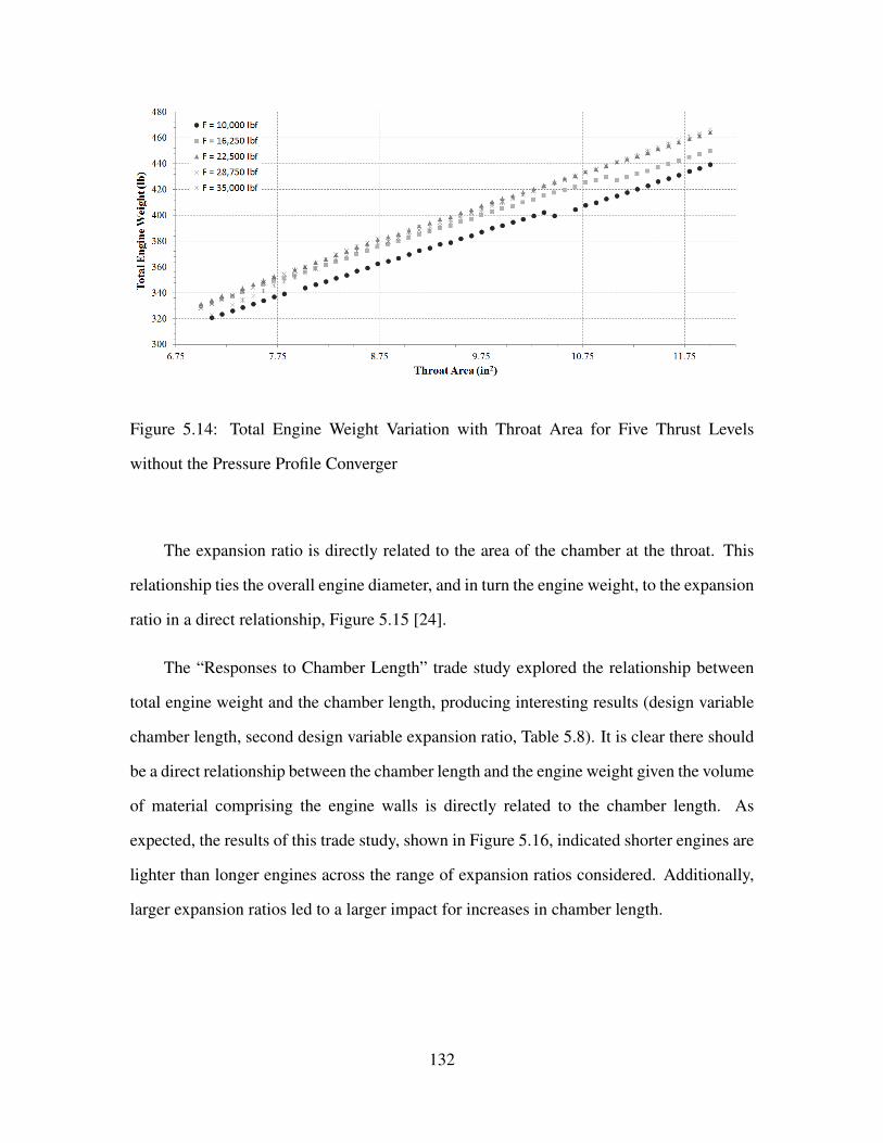
Figure 5.14: Total Engine Weight Variation with Throat Area for Five Thrust Levels

without the Pressure Profile Converger

The expansion ratio is directly related to the area of the chamber at the throat. This

relationship ties the overall engine diameter, and in turn the engine weight, to the expansion

ratio in a direct relationship, Figure 5.15 [24].

The “Responses to Chamber Length” trade study explored the relationship between

total engine weight and the chamber length, producing interesting results (design variable

chamber length, second design variable expansion ratio, Table 5.8). It is clear there should

be a direct relationship between the chamber length and the engine weight given the volume

of material comprising the engine walls is directly related to the chamber length. As

expected, the results of this trade study, shown in Figure 5.16, indicated shorter engines are

lighter than longer engines across the range of expansion ratios considered. Additionally,

larger expansion ratios led to a larger impact for increases in chamber length.

132

Figure 5.15: Total Engine Weight Variation with Expansion Ratio for Five Thrust Levels

Table 5.8: Responses to Chamber Length Trade Study Design


Chamber Length (in) 6.5 20 50


Figure 5.16: Total Engine Weight Variation with Chamber Length for Five Expansion

Ratios

133

The trade study “Responses to Characteristic Length” looked at the relationship

between total engine weight and the characteristic length. The design variable in this

pairwise relationship was the characteristic length. The second design variable for this

trade study was the expansion ratio (Table 5.9).

Table 5.9: Responses to Characteristic Length Trade Study Design


Characteristic Length (in) 35 100 50


The characteristic length, shown in Equation (5.10), is the ratio of the chamber volume

to the throat area. Typical values for characteristic length vary from 30 inches to 100

inches. Generally, smaller values for characteristic length lead to smaller, and lighter

weight, engines. However, there is a minimum acceptable value for characteristic length for

a given propellant combination based on the combustion residence time, below which the

combustion will not be complete. For chambers with a constant cylindrical cross-section,

the relationship between the characteristic length and the chamber volume leads to a direct

relationship between the characteristic length and the chamber diameter [5].

L∗ = Vc/At (5.10)

However, for the DEAN, the chamber diameter is not related to the characteristic

length. Instead, the chamber diameter is determined by the expansion ratio and the throat

area. The characteristic length determines the diameter of the aerospike within the chamber.

This inverse relationship is shown in Figure 5.17. Increases in chamber volume due to

increases in the characteristic length (with the chamber diameter fixed) must be accounted

for by decreases in the aerospike diameter. These decreases can be dramatic, with a

134

decrease in characteristic length of 65 inches resulting in an increase in the space between

the chamber and aerospike walls of 1.6 inches for the base trade study design.

(a) L∗ = 35 in (b) L∗ = 100 in

Figure 5.17: Impact of Characteristic Length on DEAN Geometry

The engine weight decreased initially and then followed the expected direct

relationship with the characteristic length, Figure 5.18. Inspection of the aerospike

geometry data in the trade study results showed the cause of the initial decrease in

engine weight. The results in Figure 5.19 show the aerospike wall thickness varied with

characteristic length, first decreasing over an initial range of characteristic lengths, then

settling to a constant value. This transition to a constant wall thickness was the result

of competing design objectives in the structural jacket sizing in the simulation. The first

objective is to minimize the wall thickness based on the stresses in the wall as calculated

by Equation (5.11) and Equation (5.12). The second objective is to create a uniform bore

in the aerospike to simplify manufacturing while reducing the weight of the aerospike by

removing unnecessary material. As the characteristic length increases, the driving factor

between these two objectives switched from minimizing the wall thickness to simplifying

the manufacturing, leading to a constant wall thickness.

135

Figure 5.18: Total Engine Weight Variation with Characteristic Length for Five Expansion

Ratios

σt =pir2

i − por2o − r2

i r2o(po − pi)/r2

r2o − r2

i

(5.11)

σr =pir2

i − por2o + r2

i r2o(po − pi)/r2

r2o − r2

i

(5.12)

Further inspection of the results indicated larger expansion ratios lead to thicker

aerospikes as shown in the figure. This result is driven by stresses in the wall. The larger

expansion ratios led to larger aerospike radii, and larger radii led to higher stresses in the

aerospike wall. The structural jacket sizing analysis compensated for the increased stresses

by increasing the wall thickness.

The transitions to constant values for aerospike thickness corresponded to the

transition in the total engine weight from an inverse relationship with the characteristic

length to a direct one. These results indicate the weight savings from the reduced

136

Figure 5.19: Aerospike Thickness Variation with Characteristic Length for Five Expansion

Ratios

aerospike wall thickness exceeded the weight growth otherwise associated with increase

in characteristic length and explain the observed deviation from expected relationship.

The DEAN simulation predicted weight is consistent with liquid rocket engine theory

with respect to throat area, expansion ratio, chamber length, and characteristic length. The

study of the throat area relationship demonstrated the impact of scaling the turbopumps for

each design. Also, studying the characteristic length demonstrated the differences between

the DEAN’s chamber design and traditional constant cross-section cylindrical chambers.

5.4.2 Scalability of the DEAN.

The common unanswered question in previous generations of DEAN research was “is

the DEAN scalable?”. Previous results were unclear regarding how flexible the DEAN

architecture was in terms of varying geometry and performance. Using the improvements

in the current DEAN simulation, the trade studies above demonstrated the DEAN is quite

scalable. Table 5.10 summarizes the ranges for the DEAN’s key design variables. The

137

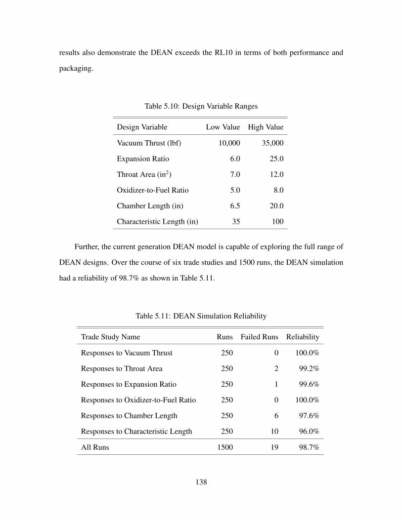
results also demonstrate the DEAN exceeds the RL10 in terms of both performance and

packaging.

Table 5.10: Design Variable Ranges

Design Variable Low Value High Value

Vacuum Thrust (lbf) 10,000 35,000

Expansion Ratio 6.0 25.0

Throat Area (in2) 7.0 12.0

Oxidizer-to-Fuel Ratio 5.0 8.0

Chamber Length (in) 6.5 20.0

Characteristic Length (in) 35 100

Further, the current generation DEAN model is capable of exploring the full range of

DEAN designs. Over the course of six trade studies and 1500 runs, the DEAN simulation

had a reliability of 98.7% as shown in Table 5.11.

Table 5.11: DEAN Simulation Reliability

Trade Study Name Runs Failed Runs Reliability

Responses to Vacuum Thrust 250 0 100.0%

Responses to Throat Area 250 2 99.2%

Responses to Expansion Ratio 250 1 99.6%

Responses to Oxidizer-to-Fuel Ratio 250 0 100.0%

Responses to Chamber Length 250 6 97.6%

Responses to Characteristic Length 250 10 96.0%

All Runs 1500 19 98.7%

138

5.4.3 DEAN Thrust-to-Weight Ratio and Turbopump Power.

Comparing previous results to the RL10 confirmed expectations about the DEAN

architecture in terms of thrust-to-weight and the power available to the turbopumps. The

three designs from previous DEAN research were reevaluated using the fourth generation

DEAN model to generate a consistent set of data to compare to the RL10 family of engines.

Table 5.12 lists the thrust-to-weight ratio and the LH2 pump power for three generations

of the RL10 and the first three generations of the DEAN. In each comparison, the DEAN

exhibited the expected increase in pump power from the second cooling loop. This increase

is dramatic, yielding over four times the power of the RL10A-3, while still remaining

under the 5900 HP demonstrated by Pratt and Whitney as part of the an upper stage

demonstrator engine [25]. Similarly, the DEAN showed the expected improvements in

thrust-to-weight ratio over the RL10 family. Further, while previous DEAN results fell

short of the vacuum specific impulse of the RL10, results from the performance trade

studies above demonstrated the DEAN can match or exceed the RL10 with the appropriate

designs.

Table 5.12: Comparison of RL10 Engine Family to DEAN Designs

Engine FVac (lbf) Isp Vac (s) T/W LH2 Pump Power (HP)

RL10A-3 [24, 25] 16,500 444.4 53.2 789

RL10A-4 [24] 20,800 448.9 56.2 -

RL10B-2 [24] 24,750 465.5 37.3 -

Generation 1 DEAN 57,231 412.9 138.6 4562

Generation 2 DEAN 50,900 422.8 194.1 3688

Generation 3 DEAN 50,161 425.7 163.9 3340

139

5.5 Conclusion

The results of this study support four key conclusions. First, the DEAN architecture,

utilizing an aerospike nozzle to implement a dual-expander cycle, is feasible and delivers

improved performance over single expander cycle engines in a compact package. The

DEAN architecture consistently achieved thrust-to-weight ratios well in excess of the

design goal of 106.5 and vacuum thrust levels of 50,000 lbf. These designs were also

compact, ranging in length from 27 to 38 inches.

Second, the DEAN’s simulation is consistent with the scientific and engineering

principles of rocket propulsion. A series of six trade studies over a wide range of designs

and performance levels verified its performance.

Third, the DEAN exceeds the performance of the RL10 for comparable thrust levels.

Comparison of previous generation designs to the RL10 showed the DEAN’s second

cooling loop gives it more than four times the pumping power of the RL10A-3 and more

than twice the thrust-to-weight ratio of the RL10A-4 and RL10B-2. Trade study results

showed the increased pumping power gives the DEAN more than twice the chamber

pressure of the RL10A-4 and RL10B-2 while being less than half the length.

Fourth, the DEAN architecture is ready for mission specific comparisons to existing

upper stage engines. Trade studies have verified the DEAN’s architecture and demonstrated

its advantages over single expander cycle engines. Further, the results of these trade

studies have also demonstrated the current DEAN simulation has the required flexibility

and robustness for use in engineering optimization studies.

140

VI. Fourth Generation DEAN Materials

6.1 Introduction

One of the key aspects of the third generation DEAN research was an initial study

on the impact of material selection on the DEAN’s thrust-to-weight ratio. This study

was performed by J. Hall for the third generation DEAN design and was implemented

by parametrically varying the material selection for each of the seven engine components

in the DEAN model which have material options. This study focused on the materials

selection for a single DEAN design. The results of the study indicated the chamber should

use silicon carbide for its cooling jacket and aluminum 7075 T6 for its structural jacket. The

aerospike nozzle should be fabricated from a single material, oxygen-free copper (C10100)

[4].

With the fourth generation DEAN simulation’s ability to model a wide range of engine

designs, it is critical to ensure the DEAN’s materials selection performs well across the

range of designs under consideration. This chapter covers the process and results used in

an updated materials selection study. This study began by optimizing the cooling channel

designs for both the chamber and aerospike cooling channels to ensure the cooling channels

provide a high degree of cooling while minimizing the fluid Mach numbers in the channels

over a wide range of engine designs. The study then examined the material choices for the

DEAN using designs of experiments covering a variety of engine designs with significant

influence on component weight.

6.2 Background

6.2.1 Cooling Channel Design Constraints.

From the beginning DEAN research has targeted reusability as one of its objectives.

During the first generation DEAN research, this objective was met by constraining the

141

cooling jacket wall temperatures to 50% of the melting point for the selected material [2].

The third generation DEAN research indicated this requirement was overly conservative

and so it was modified to 60% of the melting point [4].

Constraints on the maximum Mach number in the cooling channels have been

consistently used to ensure shock waves do not form in the cooling channels, increasing

the risk of catastrophic failure. The requirements are the maximum Mach number in the

LOX cooling channels must be less than or equal to 0.6 and the maximum Mach number

in the LH2 cooling channels must be less than or equal to 0.9 [2].

6.2.2 Third Generation DEAN Materials Selection.

The materials selection study for the third generation DEAN design consisted of a

number of trade studies over the materials options for the DEAN. The objectives of these

trade studies were to identify the components with the greatest contribution to engine

weight and to select the best combination of materials for the DEAN in order to maximize

the thrust-to-weight ratio while considering reusability and manufacturability.

The results of these initial studies showed the chamber and aerospike structural jackets

consistently generated the greatest change in the thrust-to-weight ratio for changes in

material selection. The results also indicated the aerospike tip and plumbing have very little

influence on the total engine weight, and that they should be set to a reasonable material

selection in future optimization studies [4].

Hall concluded his materials studies by considering reuseability and manufacturabil-

ity. Plotting the variation of the wall temperatures for the chamber and aerospike cooling

jackets with the material options showed which materials met the resuseability constraint

of maintaining wall temperatures less than 60% of their melting point. From this data,

Hall concluded the copper (pure and oxygen-free) was a viable material for the aerospike

cooling jacket and silicon carbide was a viable material for both the chamber and aerospike

cooling jackets. Hall’s consideration of manufacturing concerns led him to conclude the

142

aerospike should be manufactured from a single material to simplify the machining pro-

cesses and material interfaces. Further testing indicated the only material option for the

aerospike was oxygen-free copper. Table 6.1 summarizes the final material selection for

the third generation DEAN [4].

Table 6.1: Generation 3 DEAN Materials Selection [4]

Component Material

Chamber Structural Jacket Aluminum 7075-T6

Chamber Cooling Jacket Silicon Carbide

Aerospike Structural Jacket Oxygen-Free Copper

Aerospike Cooling Jacket Oxygen-Free Copper

Aerospike Tip Oxygen-Free Copper

LOX Plumbing INCONEL 718

LH2 Plumbing INCOLOY 909

6.2.3 Cooling Channel Design.

The effectiveness of cooling jackets in liquid rocket engines is driven by the design of

the cooling channels. The number of channels and their cross-sectional areas are the two

primary factors influencing cooling channel performance. They directly influence the area

in contact with the cooling fluid. These two factors are specified by the channel ratio and

aspect ratio design variables in the model [2].

In the first generation DEAN research, Martin used varying aspect ratios along the

length of the cooling channels to balance the cooling needs with the maximum Mach

number constraints. In both cooling jackets, Martin selected low aspect ratios (shorter

channels, smaller cross-sectional area) at the throat to increase the cooling rate and higher

aspect ratios (taller channels, larger cross-sectional areas) at the end of the cooling jacket

143

to maintain a velocity below the maximum allowable Mach number. The smaller cross-

sectional area in the low aspect ratio regions increases the fluid velocity and in turn the

power required to pump the fluid. This increase in required pump power drives the solver

in the cycle model toward designs yielding more power from the turbine by increasing the

amount of heat extracted from cooling the engine, effectively increasing the cooling rate in

those regions. The larger cross-sectional areas in the high aspect ratio regions reduce the

velocity of the fluid and account for the decrease in density (increase in volume) caused

by heating the fluid. Combined, these two effects ensure the fluid stays below its Mach

number limit, preventing catastrophic failure of the engine [2].

The parametrization of the second and third generation DEAN models did not include

design variables for the cooling channels. In the second generation model, the author used

Martin’s aspect ratio schedules and computed the number of channels based on the ratios

in Martin’s design. In the third generation model, Hall used constant aspect ratios along

the length of each cooling channel and again computed the number of channels based on

the ratios in Martin’s design.

The fourth generation DEAN model includes parametrization for the cooling channels.

Eight design variables, four for each cooling jacket, control the number of channels and

the aspect ratios for the cooling channels, Table 6.2. The aspect ratio schedule generally

follows Martin’s design. Note: when the adjustment variables for a given cooling jacket

are set to a value of 1.0, the resulting cooling channels will use constant aspect ratios.

This mode of operation is included to support analyzing designs developed using the third

generation model.

144

Table 6.2: Cooling Channel Design Variables


Chamber Throat AR Aspect ratio of chamber cooling channels at the

throat

Chamber Stations Adjustment Aspect ratio multiplier for chamber cooling chan-

nels

Chamber Station 5 Adjustment Aspect ratio multiplier for chamber cooling chan-

nels at station 5

Chamber Cooling Channels Ratio Ratio of the number of chamber cooling channels

to the chamber circumference at the throat

Nozzle Throat AR Aspect ratio of aerospike cooling channels at the

throat

Nozzle Station 1 Adjustment Aspect ratio multiplier for aerospike cooling

channels at stations 1 and 2

Nozzle Station Spike Adjustment Aspect ratio multiplier for aerospike cooling

channels at stations 7 and 8

Aerospike Cooling Channels Ratio Ratio of the number of aerospike cooling channels

to the nozzle circumference at the throat

145

6.3 Designing the DEAN Cooling Channels for Fourth Generation DEAN Model

The cooling channel design study was conducted using a series of designs of

experiment (DOE), parametric studies, and optimization studies. All of these trade studies

used a common base design shown in Table 6.3. The cooling channel design study was

conducted in three phases. The first phase used three designs of experiments to identify the

design variables with significant influence on the cooling channel performance. The second

phase used a series of parametric studies and optimization studies to determine values for

the key channel design variables, yielding designs for the cooling channels performing well

across a range of engine designs. Finally, the third phase verified the results of the second

phase by testing them at four engine designs representing a cross section of the DEAN

trade space.

146

Table 6.3: Cooling Channel Design Study Base Design

Variable Value
















Chamber Structural Jacket Material Silicon Carbide

Chamber Cooling Jacket Material Silicon Carbide

Aerospike Structural Jacket Material Silicon Carbide

Aerospike Cooling Jacket Silicon Carbide

Aerospike Tip Material Silicon Carbide



147

6.3.1 Phase I - Identify Key Design Variables.

In order to identify the key design variables, three distinct designs of experiments

(DOE 1, DOE 2, DOE 3) were employed. All three designs of experiments were based

on the trade studies used in the system level verification tests. The ranges for the design

variables were developed to maximize the range of designs considered and the reliability

of the model execution. All trade studies used a randomized space filling design covering

250 points made up of a 125 Design Explorer Orthogonal Array with 125 additional points

from a Latin-Hypercube unless otherwise specified. The results of the three DOEs are

shown in Figure 6.1, Figure 6.2, and Figure 6.3 below. The rows list the design variables

and the columns list the response variables. Cells with an ’X’ in them indicate the design

variable for that row has a significant influence on the response variable in that column.

The relationships were determined using ModelCenter’s Variable Influence Profiler. The

Variable Influence Profiler uses Analysis of Variance methods over a Kriging model of the

data to compute variable importance levels [67].

The objective of DOE 1 (Table 6.4) was to determine which system level design

variables have significant influence on the heat transfer (i.e. wall temperature) and

maximum Mach numbers in the cooling channels. The influence of the system level design

variables on sizing of the structural jackets and plumbing was also investigated for use in

the materials selection trade studies. These key system level design variables will be used

in later trade studies to create the range of engine configurations for both designing the

cooling channels and selecting materials for the primary DEAN components.

The results of DOE 1 are shown in Figure 6.1. The vacuum thrust and throat area

showed considerable influence on the wall temperatures for both the chamber and the

aerospike. The vacuum thrust and expansion ratio influenced the maximum Mach numbers

most significantly. Historically, ensuring the cooling channels meet the maximum Mach

number constraints is easier than the wall temperature constraints. So the remaining designs

148

of experiments emphasized engine designs which drive the wall temperatures by varying

vacuum thrust and throat area.

Table 6.4: Design Variables for Cooling Channel Design Study DOE 1 - Influence of

System Level Design Variables


Expansion Ratio 6 25 Space Filling

Throat Area (in2) 7 10 Space Filling

Chamber Length (in) 10 15 Space Filling

Characteristic Length (in) 35 75 Space Filling

Vacuum Thrust (lbf) 10,000 35,000 Space Filling

Oxidizer-to-Fuel Ratio 5 8 Space Filling

Figure 6.1: DEAN Cooling Channels Variable Influence Chart

149

DOE 2 targeted the influence of the cooling channel design variables on the LOX

cooling circuit. The four cooling channel design variables are the chamber throat AR, the

chamber stations adjustment, the chamber station 5 adjustment, and the chamber cooling

channels Ratio. Ranges for these variables are shown in Table 6.5.

Table 6.5: Design Variables for Cooling Channel Design Study DOE 2 - Chamber Channel

Design Study




Chamber Throat AR 1.2 4.0 Space Filling

Chamber Stations Adjustment 0.75 2.0 Space Filling

Chamber Station 5 Adjustment 0.75 2.9 Space Filling

Chamber Cooling Channels Ratio 10 20 Space Filling

The results of DOE 2 are shown in Figure 6.2. The station 5 adjustment had little

impact on the wall temperature or maximum Mach number. Additionally, the throat aspect

ratio and the chamber cooling channels ratio had significant influence on both the wall

temperature and the maximum Mach number in the LOX cooling channels. The chamber

stations adjustment only had significant influence on wall temperature.

150

Figure 6.2: DEAN Chamber Cooling Channels Variable Influence Chart

DOE 3 focused on the design variables for the aerospike cooling channels and their

influence. These variables are the nozzle throat AR, the nozzle station 1 adjustment, the

nozzle station spike adjustment, and the aerospike cooling channels ratio (Table 6.6). DOE

3 (Figure 6.3) indicates the spike adjustment had little impact on the wall temperature or

maximum Mach number. Additionally, the throat aspect ratio and the aerospike cooling

channels ratio had significant influence on both the wall temperature and the maximum

Mach number in the LH2 cooling channels, while the nozzle station 1 adjustment only had

significant influence on wall temperature.

151

Table 6.6: Design Variables for Cooling Channel Design Study DOE 3 - Aerospike Channel

Design Study




Aerospike Throat AR 0.5 1.4 Space Filling

Aerospike Station 1 Adjustment 1.0 13 Space Filling

Aerospike Station Spike Adjustment 1.0 5.0 Space Filling

Aerospike Cooling Channels Ratio 5.0 15.0 Space Filling

Figure 6.3: DEAN Aerospike Cooling Channels Variable Influence Chart

6.3.2 Phase II - Determine Values for Design Variables.

The results of DOE 2 and DOE 3 were used to structure the process of determining

values for the cooling channel design variables by working from the least complex

decisions to the most complex decisions. The least complex decisions are for the two

152

variables which do not influence either the wall temperatures or the maximum Mach

numbers, namely the chamber station 5 adjustment and the aerospike station spike

ajustment. Both variables were arbitrarily set to 1.0 since they have no impact on the

response variables.

The next most complex decisions concern the variables only influencing one response,

namely the chamber stations adjustment and the aerospike station 1 adjustment. Both

variables only have significant influence on wall temperatures. A series of parametric

studies were run over each of these variables across a number of engine designs. The

results for all of these parametric variables indicated the same trends, Figure 6.4 and

Figure 6.5. These trends show a range of values producing a minimum wall temperature

and a minimum value for the maximum Mach number.

Figure 6.4: Chamber Wall Temperature Variation with Chamber Stations Adjustment

From these trends, values were selected to ensure the channel designs minimized the

wall temperature and maximum Mach number for a wide range of engine designs. For the

153

Figure 6.5: Chamber Maximum Mach Number Variation with Chamber Stations

Adjustment

chamber, this analysis led to a value of 1.2 for the chamber stations adjustment. For the

aerospike, this analysis led to a value of 1.7 for the aerospike station 1 adjustment.

The final four values, two for each set of cooling channels, involve the most complex

decisions. These variables influence both wall temperatures and the cooling channel Mach

numbers and for some values interact with each other. To address this complexity, the

values for these variables were determined through a pair of sequentially run optimization

problems. Each problem minimized the wall temperature and the maximum Mach numbers

by adjusting the related pair of design variables. No constraints were applied to these

optimization problems due to the significant influence of system level design variables

on the specific values for both the wall temperature and the maximum Mach numbers.

Equation (6.1) gives the mathematical definition of the optimization problem for the

chamber cooling channels and Equation (6.2) gives the mathematical definition of the

optimization problem for the aerospike cooling channels. The wall temperature was given

twice the weight of the maximum Mach number since it is historically the more challenging

154

constraint to enforce and the maximum values for the channel ratios were chosen to ensure

the minimum channel widths meet or exceed the required minimum value of 0.02 in based

on manufacturing assumptions of precision machining using a minimum tool size of 1/64

inch making two passes (one for each wall of the channel).

Find X =

Chamber Throat AR

Chamber Cooling Channels Ratio

which minimizes

f (X) = 2Tchamber wall(X) + Machchamber max(X)

where0.5

10.0

≤ X ≤

5.0

25.0

(6.1)

Find X =

Aerospike Throat AR

Aerospike Cooling Channels Ratio

which minimizes

f (X) = 2Taerospike wall(X) + Machaerospike max(X)

where0.25

5.0

≤ X ≤

2.0

15.5

(6.2)

The two optimization problems above were implemented in ModelCenter using Op-

timization Tool components. The Optimization Tool component is a built-in ModelCenter

component which uses industry standard optimization algorithms to create a loop which

drives model elements toward specified objectives. Figure 6.6 and Table 6.7 show the

cooling channel optimization model. This model runs the optimization problems in se-

ries. The loop labeled B implements Equation (6.1) and the loop labeled C implements

Equation (6.2).

155

Figure 6.6: Channel Design Optimization Model

Each embedded optimization loop consists of an Optimization Tool component and

an embedded copy of the DEAN system model. The cooling channel optimization

model uses the values from the Design Variables component (labeled A) to ensure DEAN

system models in the two optimization loops are synchronized to the same design. The

optimization model then solves for the chamber cooling channels design using the Chamber

Optimization Loop (labeled B). The optimized chamber cooling channel design is used in

the aerospike nozzle cooling channel optimization study (labeled C). The results of the

cooling channel optimization model are displayed in the Data Monitor (labeled D) and the

pressure level renderings (labeled E).

The model was run using the base design point in Table 6.2 for several starting values

of the cooling channel design variables. The results from the set of model runs clustered

around a single set of values, which were used to determine the cooling channel design

variable values shown in Table 6.8.

156

Table 6.7: Cooling Channel Optimization Model Components


A Design Variables DEAN system level design variables describing

the DEAN design for both optimization loops

B Chamber Opt Loop embedded optimization study to size the cooling

channels for the chamber

C Nozzle Opt Loop embedded optimization study to size the cooling

channels for the aerospike nozzle

C1 Chamber Opt Results ModelCenter Data Monitor displaying the results

of the chamber optimization loop

D Optimization Results ModelCenter Data Monitor displaying the final

results of the two optimization studies

E Pressure Profile Plots pressure profiles for the LOX and LH2 expander

cycles post cooling channel optimization

Table 6.8: Final Cooling Channel Design Variable Values

Variable Value









157

6.3.3 Phase III - Verification.

The results of the second phase were verified through testing and comparison to

the previous designs. The testing used four engine designs representing a cross section

of the DEAN trade space. These engines vary in vacuum thrust from approximately

16,000 lbf to 35,000 lbf and meet the physical constraints of the DEAN model. For each

engine, the design was loaded into the optimization model from the second phase and

the model was run to find updated cooling channel design variable values. The results of

these optimization studies were compared with the results using the second phase design,

Table 6.9. In all four cases, the verification run results yield slight to no reduction in

the maximum Mach numbers for the cooling channels with corresponding increases in

the wall temperatures. Given the higher priority of reducing the wall temperatures, these

results were not improvements, confirming the proposed cooling channel designs produce

universally high quality cooling channels.

Table 6.10 compares the updated cooling channel designs with Martin’s original

designs. In the chamber cooling jacket, fewer channels with lower aspect ratios are used

in the updated design to improve the thermal performance. In the aerospike cooling

jacket, a greater number of channels with a more consistent set of aspect ratios are used

to balance out the thermal performance along the entire length of the engine. These results

are consistent with the updated designs’ emphasis on thermal performance, which further

verifies the updated designs.

158

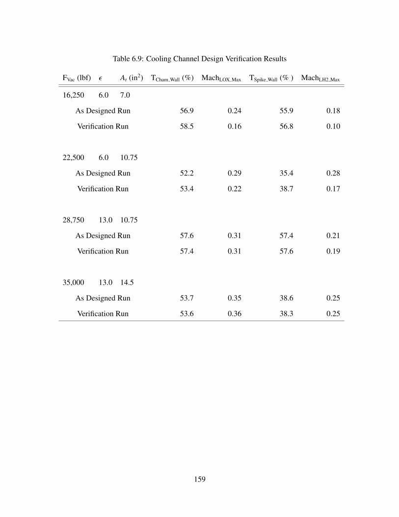
Table 6.9: Cooling Channel Design Verification Results

FVac (lbf) ε At (in2) TCham Wall (%) MachLOX Max TSpike Wall (% ) MachLH2 Max

16,250 6.0 7.0

As Designed Run 56.9 0.24 55.9 0.18

Verification Run 58.5 0.16 56.8 0.10

22,500 6.0 10.75

As Designed Run 52.2 0.29 35.4 0.28


28,750 13.0 10.75

As Designed Run 57.6 0.31 57.4 0.21


35,000 13.0 14.5

As Designed Run 53.7 0.35 38.6 0.25


159

Table 6.10: Cooling Channel Design Comparison

Station Chamber Aerospike

Martin As Designed Martin As Designed

Number of Channels

- 785 654 314 413

Aspect Ratios

1 3.57 1.50 5.00 1.46

2 2.86 1.20 5.00 1.46

3 2.86 1.20 3.20 1.26

4 2.86 1.20 1.71 1.06

5 3.33 1.00 0.67 0.86

6 3.00 1.00 0.57 0.86

7 - - 0.67 0.86

8 - - 1.33 0.86

6.4 Materials Selection Study

The materials selection study was carried out as a series of trade studies over the

material options for each relevant DEAN component. The objective of the materials

selection trade studies was to find the “best materials selection” for the overall DEAN

architecture. The “best materials selection” was defined as the materials selection yielding

consistently low weight engines over a wide range of designs. Using this definition,

optimal materials are ones producing tightly clustered data points with low values on

weight variation with material selection plots. Conversely, materials are not considered

optimal if they produce a wide range of engine weights, even when some of those weights

160

may be lower than optimal materials. This distinction ensures the selected materials are

globally optimal instead of locally optimal depending on the selected DEAN design.

The results of the cooling channel design study drove the materials selection study.

First the new cooling channel designs were incorporated into a base design for the trade

studies in the materials selection study. This design is summarized in Table 6.11.

Next, the results of the cooling channel design studies, indicating which design

variables have significant influence on the cooling jacket wall temperatures, the structural

jacket sizes, and the weight of the plumbing, were used to design the individual materials

selection trade studies to ensure a wide range of relevant engine designs were considered.

The throat area and the vacuum thrust showed the most influence on the wall temperatures.

The expansion ratio and the vacuum thrust had the greatest influence on the structural jacket

sizes. Additionally, the cooling channel design studies indicated the expansion ratio and

vacuum thrust drive the plumbing weight.

Before beginning the materials selection trade studies, the third generation DEAN

material list was filtered to eliminate extraneous material options. This filtering included

removal of materials for manufacturing and modeling reasons. Silicon carbide was

removed as an option for structural jackets and the aerospike tip to limit the amount of

ceramic material required to manufacture the DEAN. The material lists for the aerospike

structural jacket and aerospike tip were configured to use the same material for both

elements to simplify the manufacturing process and reduce the number of materials in any

given DEAN design. Oxygen-free copper was removed as an option for cooling jackets

because thermal conductivity was not available over the necessary range of temperatures.

Beryllium copper was removed completely as no data was found detailing the temperature

impacts on ultimate and yield strengths. Table 6.12 lists the DEAN components and the

materials available for each one.

161

Table 6.11: Materials Studies Base Design

Variable Value
















Chamber Structural Jacket Material Silicon Carbide

Chamber Cooling Jacket Material Silicon Carbide

Aerospike Structural Jacket Material Silicon Carbide


Aerospike Tip Material Silicon Carbide



162

Table 6.12: Materials Options for DEAN Components

Component Materials

Chamber Structural Jacket Copper, INCOLOY 909, INCONEL 718, INCONEL

625, Alloy 188, Aluminum 7075 T6, Aluminum 2024

T6, Oxygen-Free Copper, Titanium, Cobalt

Chamber Cooling Jacket Copper, Silicon Carbide, INCOLOY 909, INCONEL

718, INCONEL 625, Alloy 188, Cobalt

Aerospike Structural Jacket & Tip Copper, INCOLOY 909, Alloy 188, Oxygen-Free

Copper, Cobalt

Aerospike Cooling Jacket Copper, Silicon Carbide, INCOLOY 909, Alloy 188,

Cobalt

LOX Plumbing Copper, INCOLOY 909, INCONEL 718, INCONEL

625, Alloy 188, Oxygen-Free Copper, Cobalt

LH2 Plumbing Copper, INCOLOY 909, Alloy 188, Oxygen-Free

Copper, Cobalt

For each material selection trade study, a design of experiments was configured with

a parameter scan of the available materials for the component under consideration. To

ensure the results were valid for a wide range of engines, the design of experiments also

included the design variables with significant influence on the weight of the component

being studied as determined by the cooling channel design studies. These trade studies are

technically parameter scans as the material selection is a discreet variable. However, they

may be treated as full factorial designs since the trade study tests all available combinations

of engine designs.

The chamber cooling jacket material was tested first using the throat area and vacuum

thrust to vary engine designs (Table 6.13). Of the material options for the chamber cooling

163

jacket (Figure 6.7), only one, silicon carbide, consistently yielded values below the melting

point, with many of designs falling below the 60% of melting point constraint, indicating

silicon carbide is the only viable material option for the chamber cooling channel. This

result matches the third generation DEAN results.

Table 6.13: Design Variables for Chamber Cooling Jacket Material Study




Chamber Cooling Jacket Material - - Parameter Scan

Figure 6.7: Chamber Percent Melting Point Variation with Material for Various Throat

Areas and Thrust Levels

The aerospike cooling jacket material was tested next varying the engine designs using

the throat area and vacuum thrust (Table 6.14). As with the chamber cooling jacket, the only

164

material which consistently yielded values below the melting point, with many of designs

falling below the 60% of melting point constraint, was silicon carbide, Figure 6.8. This

result differs from the third generation DEAN material selection of oxygen-free copper.

Table 6.14: Design Variables for Aerospike Cooling Jacket Material Study




Aerospike Cooling Jacket Material - - Parameter Scan

Figure 6.8: Aerospike Percent Melting Point Variation with Material for Various Throat

Areas and Thrust Levels

The third material study tested the chamber structural jacket material using the

expansion ratio and vacuum thrust to vary engine designs (Table 6.15). Figure 6.9 and

Figure 6.10 show large ranges for the results. The structural jacket wall thickness varied

165

from under 1.0 in to well over the 2.5 in shown. Similarly, the structural jacket weight

varied from under 9 lbf to more than the 500 lbf in the figure. For both the wall thickness

and the weight, two materials stood out as candidates: INCOLOY 909 and INCONEL

718. They both produced low weight designs with little variation across engine designs.

However, INCONEL 718 is also the material proposed for use in the LOX pump and the

LOX plumbing [4, 26], so selecting it for the structural jacket would yield a single metal

for all LOX components, eliminating the need to mitigate galvanic corrosion. Further,

INCONEL 718 is compatible with LOX so the chamber cooling jacket would not require

a cover. This material selection is a change from the Aluminum 7075-T6 selected in the

third generation DEAN research.

Table 6.15: Design Variables for Chamber Structural Jacket Material Study


Expansion Ratio 6.0 25.0 3


Chamber Structural Jacket Material - - Parameter Scan

166

Figure 6.9: Chamber Structural Jacket Thickness Variation with Material Selection for

Various Expansion Ratios and Thrust Levels

Figure 6.10: Chamber Structural Jacket Weight Variation with Material Selection for


The aerospike structural jacket material was tested next using the expansion ratio and

vacuum thrust to vary engine designs (Table 6.16). As discussed above, the aerospike tip

167

was set to the same material as the aerospike structural jacket. Figure 6.11 and Figure 6.12

display the results of aerospike structural jacket material study. For both the wall thickness

and the total aerospike weight one material stood out as a candidate material: INCOLOY

909. The INCOLOY 909 produced low weight aerospikes with little variation across engine

designs. Further, INCOLOY 909 is compatible with LH2, so the aerospike cooling jacket

would not require a cover. INCOLOY 909 is also the previously selected LH2 plumbing

material, and selecting the same metal for all of the LH2 components eliminates the need

to mitigate galvanic corrosion.

Table 6.16: Design Variables for Aerospike Structural Jacket Material Study




Aerospike Structural Jacket Material - - Parameter Scan

The results confirmed the third generation DEAN research indicating material

selection for the aerospike tip has little influence on its weight, Figure 6.13. Across the

range of material options, the aerospike tip weight stayed within the range of 5 lbf to 50

lbf, varying due more to the aerospike geometry than due to the material selection. The

selection of INCOLOY 909 for the aerospike structural jacket and tip is a change from the

oxygen-free copper selected in the third generation DEAN research.

168

Figure 6.11: Aerospike Structural Jacket Thickness Variation with Material Selection for


Figure 6.12: Aerospike Weight Variation with Material Selection for Various Expansion

Ratios and Thrust Levels

169

Figure 6.13: Aerospike Tip Weight Variation with Material Selection for Various Expansion

Ratios and Thrust Levels

The fifth material study tested the LOX plumbing material using the expansion ratio

and vacuum thrust to vary engine designs (Table 6.17). The LOX plumbing weight

(Figure 6.14) accounted for between 2% and more than 30% of the engine’s weight.

INCONEL 718, the material selected during the third generation DEAN research, was

among best performing materials over the full range of engine designs and has already

shown to perform well in the other LOX components (pump and chamber structural jacket),

confirming its selection as the LOX plumbing material.

Table 6.17: Design Variables for LOX Plumbing Material Study




LOX Plumbing Material - - Parameter Scan

170

Figure 6.14: LOX Plumbing Weight Variation with Material Selection for Various

Expansion Ratios and Thrust Levels

The LH2 plumbing material was tested last using the expansion ratio and vacuum

thrust to vary the engine designs (Table 6.18). The LH2 plumbing weight (Figure 6.15)

accounted for between 2% and more than 50% of the engine’s weight. One option stands

out as a candidate material: INCOLOY 909. The data points for INCOLOY 909 are tightly

clustered indicating the change in plumbing weight is very small compared to changes in

engine designs. This selection matches the results in the third generation DEAN research.

Table 6.18: Design Variables for LH2 Plumbing Material Study




LH2 Plumbing Material - - Parameter Scan

171

Figure 6.15: LH2 Plumbing Weight Variation with Material Selection for Various

Expansion Ratios and Thrust Levels

Table 6.19 summarizes the results of the materials selection study. It includes the use

of silicon carbide for both the chamber and aerospike cooling jackets, the use of INCONEL

718 for the chamber structural jacket and LOX plumbing, and the use of INCOLOY 909

for the aerospike structural jacket and tip and the LH2 plumbing. It also includes an update

to the cooling channel geometry option to use the structural jacket as the cooling jacket

cover as both structural jackets are now compatible with the fluids in the cooling jackets.

172

Table 6.19: Generation 4 DEAN Design Materials Selection

Component Material

Chamber Structural Jacket INCONEL 718


Aerospike Structural Jacket INCOLOY 909


Aerospike Tip INCOLOY 909



Cooling Geometry Option Structural Jacket is Cover

6.5 Conclusion

The materials study yielded an updated materials selection covering a wide range of

engine designs. The materials study also confirmed the following findings from previous

research: the aerospike tip material selection has little influence on the engine’s thrust-

to-weight ratio, the chamber cooling jacket should be manufactured from silicon carbide,

the LOX plumbing should be manufactured from INCONEL 718, and the LH2 plumbing

should be manufactured from INCOLOY 909. The material study also found material

selections for the aerospike cooling jacket (silicon carbide), chamber structural jacket

(INCONEL 718), and the aerospike structural jacket (INCOLOY 909) which produced low

weight engines across a wide range of designs compared to previous material selections.

173

VII. Optimization Studies of Dual-Expander Aerospike Nozzle Upper Stage Rocket

Engine

The text of this chapter was submitted to the AIAA Journal of Spacecraft and Rockets

in July 2014. It is unaltered from the submitted version except in its formatting as required

by the AFIT dissertation style guide.

7.1 Introduction


is estimated to be as much as $10,000 per pound [15]. These costs mean placing satellites

in orbit costs hundreds of millions of dollars. Savings from improved thrust-to-weight ratio

and specific impulse can be significant. However, achieving these gains in performance will

require more than incremental improvements in rocket engine technology. The thrust-to-

weight ratio of high powered liquid rocket engines has been relatively constant with respect

to propellant selection for decades, regardless of thrust levels and designs [23].

The Air Force Institute of Technology (AFIT) is researching a modification to the

expander cycle as a means of breaking the performance barrier. The result of this

research is the Dual-Expander Aerospike Nozzle (DEAN) rocket engine (Figure 7.1).

The DEAN is a liquid oxygen (LOX)/liquid hydrogen (LH2) reusable upper stage engine

offering performance advantage over traditional upper stage engines in a compact package

leading to dramatically improved thrust-to-weight ratios while maintaining a vacuum

specific impulse comparable to current LOX/LH2 upper stage engines. AFIT’s goal with

its research into the DEAN is to determine the viability of the DEAN architecture by

finding those missions and designs for which the DEAN has a competitive advantage over

traditional upper stage engines. Additionally, the DEAN architecture is a forerunner to a

174

similar boost stage architecture, where the aerospike nozzle’s global performance could

result in event greater performance gains.

Figure 7.1: The Dual-Expander Aerospike Nozzle Upper Stage Engine

7.2 Background


The DEAN architecture, shown in Figure 7.2, uses two novel design choices. The first

is the use of separate expander cycles for the fuel and the oxidizer. In a traditional expander




In the DEAN, the fuel and oxidizer each drive their own turbines and power their own

pumps.


nozzle. Aerospike nozzles are a center body in the combusted propellant flow often forming

175


the inner wall of the chamber. The ambient atmosphere forms the outer boundary for the

flow for these nozzles. The combusted propellant flow expands against the aerospike nozzle

and radially outward to match ambient pressure at each location in the nozzle flow field.

The interaction with the ambient atmosphere gives aerospike nozzles altitude compensation

ability, making them more efficient as altitude changes for the rocket. Similar bell nozzles

must be designed for a single, specific altitude [24]. In the DEAN, the use of an aerospike

nozzle provides a second, physically separate cooling loop from the chamber for use in the

fuel expander cycle, greatly simplifying the implementation of a dual-expander cycle.

The second cooling loop increases the surface area inside the chamber, transferring

greater energy to the propellants and providing more power to the turbines when compared

to traditional expander cycle engines such as the RL10. This increased power is

transferred to the pumps and in turn leads to increased chamber pressures. The increase in

176

chamber pressure yields engine performance improvements. This improved performance

(thrust/weight) leads to smaller engines, in terms of both weight and physical dimensions,

for similar levels of thrust and specific impulse. The separate expander cycles also ensure

the fuel and oxidizer remain physically separated until entering the combustion chamber,

eliminating the catastrophic failure mode in traditional expander cycles; failure of an inter-

propellant seal [2, 25–27].

The DEAN architecture is not without its challenges, though. For example, the LOX

cycle requires a turbine material capable of operating in an oxygen environment. Material

surveys at AFIT have shown Inconel 718 provides both satisfactory oxygen resistance and

suitable mechanical performance for use in both the pump and the turbine in the LOX cycle

[26]. Also, the expansion ratio of aerospike nozzles is limited by the chamber geometry

as shown in Equation (7.1) [4, 24]. Due to this limit, aerospike nozzles generally need

larger chamber diameters to reach useful expansion ratios, potentially limiting the range of

engines which offer improved thrust-to-weight while also delivering the required specific

impulse.

εaerospike =Ac throat

At(7.1)

7.2.2 Previous Research.

The current research builds on three generations of DEAN simulations. The

performance goals for the DEAN have been a vacuum thrust of 50,000 lbf, a vacuum

specific impulse of 464 s, and a thrust-to-weight ratio of 106.5. All three generations use

NASA’s Numerical Propulsion System Simulation (NPSS) to explore cycle performance.

NPSS is a computer simulation tool for modeling aircraft and rocket engines developed by

the NASA Glenn Research Center with assistance from the aerospace propulsion industry.

Engine simulations built in NPSS provide higher fidelity results than engine cycle studies

[31]. The DEAN cycle simulation balances the fluid flows, mechanical power, and thermal

177

flows in the two expander cycles to converge on the engine performance parameters for a

given design point.

Two of the three previous DEAN simulations extended the cycle model by embedding

it into a system level engine simulation built in Phoenix Integration’s ModelCenter.

ModelCenter is a multidisciplinary modeling environment used to study the trade space

of and optimize a design. ModelCenter can combine analyses developed in a variety of

tools including MATLAB, Mathcad, Excel, and command line executables into a single

system level simulation [60]. The system level DEAN simulation includes a parameterized

version of the cycle model and connects it to additional analyses to estimate the DEAN’s

geometry and weight in order to compute the DEAN’s physical dimensions and thrust-to-

weight ratio.

The first generation research focused on developing the initial cycle balance of the

DEAN for a single design. This design, shown in Figure 7.3(a), included an assumed

expansion ratio of 125, producing a vacuum thrust of over 57,000 lbf and a vacuum

specific impulse of 472 s with a thrust-to-weight ratio of 119 [2]. The second generation

research implemented parametric modeling of the DEAN by refactoring the cycle model

and integrating it into the first system level simulation. The new DEAN simulation retained

the assumed expansion ratio. Through a series of trade studies, a new scaled DEAN was

developed to more closely match the original design goals. The resulting design, shown

in Figure 7.3(b), had a vacuum thrust of 50,900 lbf and a vacuum specific impulse of 489

s, while being 25% shorter in total length and reducing the size of the turbomachinery

[27]. The third generation research extended the system simulation to include additional

calculations including materials options, structural sizing, nozzle contour, and engine

weight. The third generation DEAN research also moved from an assumed value for

the expansion ratio to a calculated value based on the DEAN’s geometry, resulting in

lower values for the vacuum specific impulse. The final design for the third generation

178

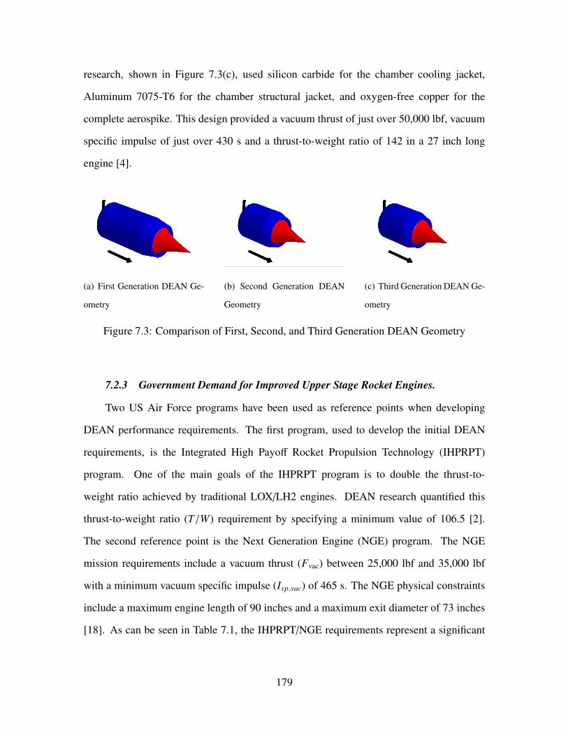
research, shown in Figure 7.3(c), used silicon carbide for the chamber cooling jacket,

Aluminum 7075-T6 for the chamber structural jacket, and oxygen-free copper for the

complete aerospike. This design provided a vacuum thrust of just over 50,000 lbf, vacuum

specific impulse of just over 430 s and a thrust-to-weight ratio of 142 in a 27 inch long

engine [4].


ometry


Geometry


ometry


7.2.3 Government Demand for Improved Upper Stage Rocket Engines.

Two US Air Force programs have been used as reference points when developing

DEAN performance requirements. The first program, used to develop the initial DEAN

requirements, is the Integrated High Payoff Rocket Propulsion Technology (IHPRPT)

program. One of the main goals of the IHPRPT program is to double the thrust-to-

weight ratio achieved by traditional LOX/LH2 engines. DEAN research quantified this

thrust-to-weight ratio (T/W) requirement by specifying a minimum value of 106.5 [2].

The second reference point is the Next Generation Engine (NGE) program. The NGE

mission requirements include a vacuum thrust (Fvac) between 25,000 lbf and 35,000 lbf

with a minimum vacuum specific impulse (Isp vac) of 465 s. The NGE physical constraints

include a maximum engine length of 90 inches and a maximum exit diameter of 73 inches

[18]. As can be seen in Table 7.1, the IHPRPT/NGE requirements represent a significant

179

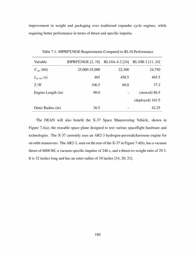
improvement in weight and packaging over traditional expander cycle engines, while

requiring better performance in terms of thrust and specific impulse.

Table 7.1: IHPRPT/NGE Requirements Compared to RL10 Performance

Variable IHPRPT/NGE [2, 18] RL10A-4-2 [24] RL10B-2 [11, 24]

Fvac (lbf) 25,000-35,000 22,300 24,750

Isp vac (s) 465 450.5 465.5

T/W 106.5 60.8 37.3

Engine Length (in) 90.0 - (stowed) 86.5

(deployed) 163.5

Outer Radius (in) 36.5 - 42.25

The DEAN will also benefit the X-37 Space Maneuvering Vehicle, shown in

Figure 7.4(a); the reusable space plane designed to test various spaceflight hardware and

technologies. The X-37 currently uses an AR2-3 hydrogen-peroxide/kerosene engine for

on orbit maneuvers. The AR2-3, seen on the rear of the X-37 in Figure 7.4(b), has a vacuum

thrust of 6600 lbf, a vacuum specific impulse of 246 s, and a thrust-to-weight ratio of 29.3.

It is 32 inches long and has an outer radius of 10 inches [14, 20, 21].

180

(a) X-37 Space Maneuvering Vehicle [9] (b) Rear View of X-37 Including the AR2-3

Engine [10]

Figure 7.4: X-37 Space Maneuvering Vehicle, credit US Air Force

NASA’s upper stage engine requirements are centered on the Space Launch System

(SLS). The SLS is a shuttle-derived super-heavy lift human-rated launch system which is

still in the design phase. Four upper stage configurations are being considered for the

SLS with two being relevant to DEAN research. The first of these designs, shown in

Figure 7.5(a), is an upper stage powered by four RL10 engines. This design provides a

vacuum thrust of 99,000 lbf and a vacuum specific impulse of 462.5 s, with a thrust-to-

weight ratio of 37.3. The second design, shown in Figure 7.5(b), is an upper stage powered

by a single J-2X engine providing a vacuum thrust of 294,000 lbf and a vacuum specific

impulse of 448 s, with a thrust-to-weight ratio of 55 [8, 12, 22]. Table 7.2 shows the

difference between these designs and the performance available from a single RL10B-2.

181

(a) SLS Upper Stage Design 1: Four RL10

Engines [8]

(b) SLS Upper Stage Design 2: Single J-2X

Engine [8]

Figure 7.5: SLS Upper Stage Designs, credit The Boeing Corporation

182

Table 7.2: SLS Designs Compared to RL10 Performance

Variable SLS-1 [8, 11, 24] SLS-2 [12, 37] RL10B-2 [11, 24]

Engine Cycle Expander Gas Generator Expander

Fvac (lbf) 99,000 294,000 24,750

Isp vac (s) 462.5 448.0 465.5

T/W 37.3 55.0 37.3

Engine Length (in) (stowed) 86.5 180.0 (stowed) 86.5

(deployed) 163.5 (deployed) 163.5

Outer Radius (in) 108 60.0 42.25

7.3 Current Research

The fourth generation DEAN simulation builds on the lessons learned from the

previous generation models. The new simulation includes an updated geometry

parametrization, simplified structure, and a custom solver to compute initial estimates for

the cycle balance. The improvements allowed for the exploration of a wide range of designs

while improving fidelity. Figure 7.6 and Table 7.3 outline the overall structure of the fourth

generation DEAN simulation.

The updated set of parametric design variables were derived from common conceptual

design relationships. The top level design variables include the expansion ratio, the throat

area, the chamber length, the characteristic length, the vacuum thrust, and the oxidizer-

to-fuel ratio. Additional design variables include controls for the internal geometry of

the cooling channels in both expander cycles and the materials used for key DEAN

components. The response variables for the DEAN include the vacuum specific impulse,

thrust-to-weight ratio, the maximum Mach numbers in the cooling channels, the wall

temperatures of the cooling jackets, and the power required by the pumps.

183

Figure 7.6: Fourth Generation DEAN Model

After completing the fourth generation DEAN simulation, the underlying models and

the DEAN architecture were put through a detailed verification process. Inspection of

the simulation ensured source code for each module in the simulation agreed with the

underlying physics. The data flow connections between the modules were also inspected

to verify the system level model passed the correct values between modules and in turn

calculates the correct performance for the DEAN.

Following the simulation’s inspection, the DEAN architecture was verified through

a combination of inspection and testing. The inspection consisted of a detailed review

of previous research, noting where previous research demonstrated the feasibility of the

architecture, how the previous research designs compared to research objectives, and

lessons learned regarding the DEAN simulation. The testing consisted of six trade studies

comparing critical performance metrics of the DEAN to liquid rocket engine theory and

the RL10 family of upper stage engines over a wide range of DEAN designs.

The results of the six trade studies show the DEAN’s performance matched

expectations based on liquid rocket engine theory. Further, the results confirmed the

184








cycles








thicknesses


nesses and T/W




the injector face

DEAN’s advantages over single expander cycle engines. The DEAN achieved more than

double the chamber pressure of the RL10A-4 and RL10B-2. Similarly, specific impulse

results showed the DEAN can match the RL10B-2’s vacuum specific impulse in an engine

185

producing greater thrust and 80% smaller in length and diameter. The trade studies

also demonstrated the DEAN architecture is highly scalable. This scalability included

designs ranging in thrust levels from 10,000 lbf to 35,000 lbf, expansion ratios from 6.0 to

25.0. Further, the fourth generation DEAN simulation has greatly improved in robustness,

converging in 98.7% of the 1500 designs studied.

After completing the verification study, the materials selection study was updated to

cover a wide range of engine designs. The objective of this series of trade studies was

to optimize the design of the cooling channels and then the materials for each of the

major DEAN components. The updated materials selection confirmed previous research:

aerospike tip material selection has little influence on the engine’s thrust-to-weight ratio,

chamber cooling jacket should be manufactured from silicon carbide, LOX plumbing

should be manufactured from INCONEL 718, and LH2 plumbing should be manufactured

from INCOLOY 909. The results of the current research found updated material selections

for the aerospike cooling jacket (silicon carbide), chamber structural jacket (INCONEL

718), and the aerospike structural jacket (INCOLOY 909). These material selections

consistently produce low weight engines across a wide range of designs.


Comparison of the DEAN to traditional upper stage engines was carried out in three

studies. The first study looked at the US Air Force’s need for new launch capability as

expressed in the IHPRPT and NGE programs. The second study looked at the propulsion

needs on US Air Force space planes as embodied by the X-37. The final study looked

at the upper stage requirements for NASA’s SLS. All three of these studies are designed

to optimize the DEAN by maximizing its specific impulse and its thrust-to-weight ratio

subject to physical constraints and mission requirements.

Previous results showed most of the design variables have little influence on the

responses allowing fixed values to be used and moving them to the list of preassigned

186

parameters. The vacuum thrust was also considered a preassigned parameter as each

mission profile has a required vacuum thrust level. The selection of preassigned parameters

(Table 7.4) leaves five independent design variables, Table 7.5.

Each optimization study began by finding an updated base design. These new designs

were found by scaling a 20,000 lbf vacuum thrust engine. The scaling for each design

started with setting the vacuum thrust to the required mission value and then adjusting each

of the five design variables until a suitable base design was found. The updated base design

was then used for all related trade and optimization studies.

187

Table 7.4: DEAN Preassigned Parameters

Variable Value

Vacuum Thrust Mission Specific







Nozzle Stations Spike Adjustment 1.0




Cooling Geometry Option Structural Jacket is Cover

Percent Weight of Hardware 5.0

Cowl Length 0.1



Chamber Structural Jacket INCONEL 718


Aerospike Structural Jacket and Tip INCOLOY 909




188

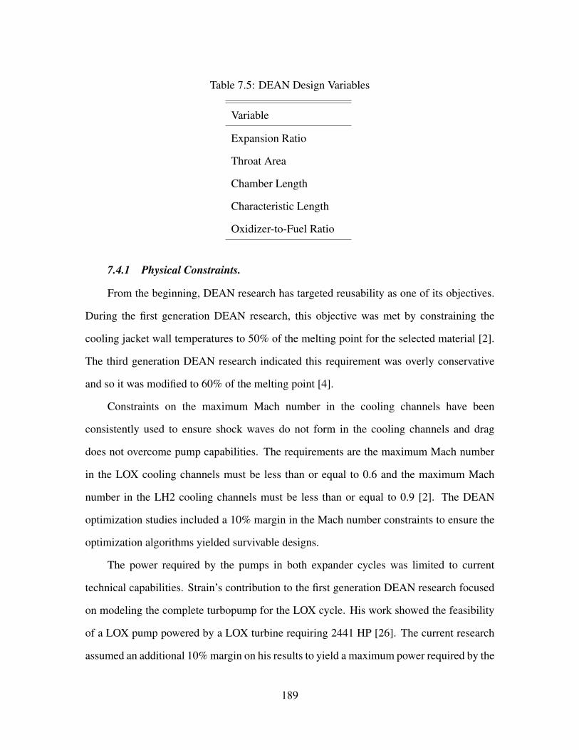
Table 7.5: DEAN Design Variables

Variable

Expansion Ratio

Throat Area

Chamber Length

Characteristic Length

Oxidizer-to-Fuel Ratio

7.4.1 Physical Constraints.

From the beginning, DEAN research has targeted reusability as one of its objectives.

During the first generation DEAN research, this objective was met by constraining the

cooling jacket wall temperatures to 50% of the melting point for the selected material [2].

The third generation DEAN research indicated this requirement was overly conservative

and so it was modified to 60% of the melting point [4].

Constraints on the maximum Mach number in the cooling channels have been

consistently used to ensure shock waves do not form in the cooling channels and drag

does not overcome pump capabilities. The requirements are the maximum Mach number

in the LOX cooling channels must be less than or equal to 0.6 and the maximum Mach

number in the LH2 cooling channels must be less than or equal to 0.9 [2]. The DEAN

optimization studies included a 10% margin in the Mach number constraints to ensure the

optimization algorithms yielded survivable designs.

The power required by the pumps in both expander cycles was limited to current

technical capabilities. Strain’s contribution to the first generation DEAN research focused

on modeling the complete turbopump for the LOX cycle. His work showed the feasibility

of a LOX pump powered by a LOX turbine requiring 2441 HP [26]. The current research

assumed an additional 10% margin on his results to yield a maximum power required by the

189

LOX pump of 2685 HP. Research and development from previous US Air Force Research

Lab programs show an LH2 pump producing 5900 HP is feasible [25].

To ensure the pressure balance produced by the NPSS model conformed to accepted

engineering practice, the pressure drop across the injector face was constrained for both the

LOX and the LH2 cycles to between 10% and 40% of chamber pressure [24].

A key manufacturing constraint for the DEAN is the difference between the outer

and inner radii at the throat. The inner and outer throat radii specify the throat area, and

changes to the throat area impact operation by leading to changes in the chamber pressure,

thrust, and specific impulse. Assuming a manufacturing tolerance for the radii at the throat

of 0.001 inch, a minimum value for the difference in throat radii of 0.1 inch limited the

variation in throat area to ±2.0%.

7.4.2 Optimizing for the IHPRPT/NGE Programs.

The first optimization study looked at the US Air Force’s need for new launch

capability as expressed in the IHPRPT and NGE programs. The objective was to maximize

the vacuum specific impulse and the thrust-to-weight ratio for DEAN engines with vacuum

thrust between 25,000 lbf and 35,000 lbf; minimum vacuum specific impulse of 465 s and

a minimum thrust-to-weight ratio of 106.5. The NGE physical constraints and maximum

exit diameter were adjusted to fit the fourth generation DEAN. The NGE requirement for

the maximum engine length of 90 inches was shortened by 25% to create a conservative

buffer for the engine mounting hardware and installation of the turbopumps. The NGE

requirement for the maximum exit diameter is the maximum outer chamber radius. The

chamber represents the largest diameter in the DEAN architecture and the model returns

radial values for this output. The base design point for the IHPRPT/NGE optimization

study used the average value for the program’s thrust range as the specified vacuum thrust

(Table 7.6).

190

Table 7.6: Base Design for IHPRPT/NGE Optimization Study

Variable Value

Design Variables







Responses



Engine Length (in) 35.4

Outer Chamber Radius (in) 8.5

Before beginning the optimization study, a final design of experiments focused on

the variable influences for the final selection of design variables. The vacuum thrust was

included in this trade study to ensure the results covered a wide range of engine designs.

The design of experiments used 500 data points made up of a 343 point Design Explorer

Orthogonal Array with 157 additional points from a Latin-Hypercube, Table 7.7.

This design of experiments yielded three key results: identification of the design

variables with significant influence on the optimization objectives and constraints,

identification of the key constraints, and selection of the optimal oxidizer-to-fuel ratio.

Figure 7.7 lists the influence of the design variables on the objectives and constraints in

the optimization problem. The rows list the design variables; columns list the response

variables. Cells with an ‘X’ indicate a significant variable influence which can vary with

191

the value of the design variable. Cells with a ‘+’ indicate a direct relationship between the

design variable and the response variable. Cells with a ‘-’ indicate an inverse relationship

between the design variable and the response variable.

Table 7.7: Design Variables for IHPRPT/NGE Optimization Study DOE 1 - Trade Space

Exploration


Expansion Ratio 15.0 25.0 Space Filling

Throat Area (in2) 9.0 13.0 Space Filling

Chamber Length (in) 7.5 13.0 Space Filling

Characteristic Length (in) 40 75 Space Filling


Oxidizer-to-Fuel Ratio 5.0 8.0 Space Filling

These relationships were determined in two phases. The first phase used ModelCen-

ter’s Variable Influence Profiler to determine the general variable influence relationships.

The Variable Influence Profiler uses Analysis of Variance methods over a Kriging model

of the trade study data to compute variable importance levels. These levels are reported

as percentages of relative importance [60]. The second phase used scatter plots to look

for consistent trends in the data between variables with significant influence relationships.

Figure 7.8 shows the inverse relationship between chamber wall temperature and the throat

area. Figure 7.9 gives an example of a strong but complex relationship between the thrust-

to-weight ratio and the characteristic length. This relationship was limited to structural and

thermal effects as the minimum characteristic length of 40 in was assumed to be sufficient

to give complete combustion yielding equilibrium products and conditions.

192

Figure 7.7: Optimization Variable Influence Chart

Figure 7.8: Chamber Wall Temperature Variation with Throat Area

The key constraints were defined by the percentages of designs violating the

constraints, Table 7.8. Note: a single design point may violate multiple constraints

193

simultaneously. The wall temperature constraints for the DEAN represented a single failure

mode where the temperatures exceed the thermal limits. Conversely, the injector face

pressure drop constraints could take the form of insufficient pressure drops, representing

operational safety concerns, or excessive pressure drops, representing inefficient designs.

All of the infeasible designs related to injector face pressure drops are of the latter variety

with the LOX pressure drops reaching as high as 60% and the LH2 pressure drops reaching

as high as 70%.

Figure 7.9: Thrust-to-Weight Ratio Variation with Characteristic Length

Table 7.8: Key Constraints for the DEAN Engine

Variable Violation Rate

Chamber Wall Temperature 20.0%

Aeropsike Wall Temperature 27.3%

LOX Injector Face Pressure Drop > 40% 22.7%

LH2 Injector Face Pressure Drop > 40% 76.2%

194

Identifying the key constraints reduced the key responses from fifteen to six: the four

key constraints plus the two objectives. The decrease is a significant reduction in the size

of the optimization problem.

Another key result from this design of experiments was the selection of an optimal

value for the oxidizer-to-fuel ratio, moving it from the list of design variables to the list

of preassigned parameters. Throughout the second and third generation DEAN research,

optimal designs have all come from using a value of 6.0 for the oxidizer-to-fuel ratio. The

fourth generation research confirmed this result for a wide range of engine designs. The

relationship between the oxidizer-to-fuel ratio and the vacuum specific impulse based on

this design of experiments resulted in a maximum specific impulse at an oxidizer-to-fuel

ratio of 6.0, Figure 7.10. The vertical bands at each oxidizer-to-fuel ratio represent changes

in the expansion ratio.

Figure 7.10: Vacuum Specific Impulse Variation with Oxidizer-to-Fuel Ratio

To confirm this conclusion, the constraints influenced by the oxidizer-to-fuel ratio

were inspected to determine any adverse affects. Of the four constraints influenced by the

195

oxidizer-to-fuel ratio, only one, the injector face pressure drop in the LH2 expander cycle

is a key constraint, Figure 7.11. The pressure drop increases approximately 5% over the

range of oxidizer-to-fuel ratios, with a value of 6.0 yielding an acceptable range for the

pressure drop. With this result being the most profound impact indicated, the conclusion

that no adverse impacts on the constraints for an oxidizer-to-fuel ratio of 6.0 is confirmed,

making it the globally optimal value for the DEAN.

Figure 7.11: LH2 Injector Face Pressure Drop Variation with Oxidizer-to-Fuel Ratio

These results provided a framework for an efficient optimization process for the

DEAN, Table 7.9. The first two steps use the variable influence and key constraints results

to address the wall temperature constraints. The wall temperatures are driven directly by

the vacuum thrust and inversely by the throat area (Figure 7.7). Therefore, missions with

higher thrusts will need larger throat areas to keep from melting the walls. However, larger

throat areas also increase the pressure drops at the injector face (Figure 7.7). Therefore,

each thrust level must be limited to the smallest throat area that yields wall temperatures

below 60% of their melting point. Using the smallest throat area possible is also consistent

196

with designing smaller engines, and in turn higher thrust-to-weight ratios [5]. The third step

uses the variable influence and key constraints results to address the other key constraints,

the injector face pressure drops, by finding the ranges of values for the expansion ratio and

chamber length yielding acceptable designs. The remaining steps combine the results from

the previous steps to define and execute the optimization problem in ModelCenter’s Darwin

optimizer. The Darwin optimizer is a trade study tool in ModelCenter implementing a

genetic optimization algorithm. The 30,000 lbf IHPRPT/NGE case will be used to present

the process.

Table 7.9: DEAN Optimization Process

Step Description

1 Set the vacuum thrust per the mission requirements/current case

2 Find the smallest throat area with the chamber and aerospike wall temperatures

below 60% of their materials’ melting points

3 Run a design of experiments over the expansion ratio and chamber length to

determine the bounds on these variables confining the trade space to designs

satisfying the key constraints

4 Create the formal definition for the multi-objective optimization problem

5 Configure the Darwin Optimizer in ModelCenter to implement the optimization

problem defined in step 4

6 Seed the Darwin Optimizer with the Pareto designs from the design of

experiments study in step 3

7 Run the Darwin Optimizer to generate the Pareto front for the design problem

defined in step 4

197

The simulation vacuum thrust was set to 30,000 lbf; the oxidizer-to-fuel ratio was

set to 6.0. Then, a parametric study was used to determine the smallest acceptable throat

area. This trade swept the throat area from 9.0 to 13.0 square inches in 0.1 square inch

increments. The wall temperature limits for both the chamber and aerospike, Figure 7.12,

resulted in a throat area of 10.7 in2, circled in the figure (1% margin for both wall

temperature constraints).

Figure 7.12: Wall Temperatures Variation with Throat Area for 30,000 lbf DEAN

The next step used a design of experiments (Table 7.10) to determine the range of

values for the expansion ratio and chamber length yielding the highest percent of valid

designs. The parameter scan design ensured the data was regularly spaced and was well

filled for both design variables.

198

Table 7.10: Design Variables for IHPRPT/NGE 30,000 lbf Step 3 DOE



Chamber Length (in) 7.0 13.0 13

In Figure 7.13 the horizontal axis is the chamber length, the vertical axis is the vacuum

specific impulse, and the axis running into the page is the expansion ratio. Points vary

directly in size with the thrust-to-weight ratio. Light gray points represent invalid designs

due to one or more constraint violations. Points highlighted with cross marks are those

points which lie on the Pareto front for the trade study results. Each of these Pareto points

represents a design which would have to decrease one of the two objectives in order to

increase the other. These points were used in the sixth step of the optimization process to

reduce the number of designs the optimization algorithm tested in order to find the global

Pareto front. The black box shows the region of the trade space bounding all of the feasible

designs and includes one step beyond the feasible range to capture any valid designs which

may be in the gap.

The fourth step in the optimization process is to formalize the optimization problem

statement. First, values which have already been determined were listed as updated

preassigned parameters. The updated preassigned parameters were the throat area,

determined in the second step, the vacuum thrust, determined by the mission/case, and

the oxidizer-to-fuel ratio. Table 7.11 lists these parameters and their values for the 30,000

lbf IHPRPT/NGE case.

Then, the optimization problem was stated mathematically: listing the objectives,

remaining design variables with their ranges, and the constraints. Equation (7.2) lists the

formal problem statement for the 30,000 lbf IHPRPT/NGE case. The ranges for the design

199

Figure 7.13: Specific Impulse Variation with Expansion Ratio and Chamber Length for

30,000 lbf DEAN

Table 7.11: Preassigned Parameters for IHPRPT/NGE 30,000 lbf Optimization Study

Variable Value




variables have been limited to discreet steps to facilitate the use of the selected genetic

optimization algorithm for efficiency [60]. The throat area and chamber length varied in

200

increments of 0.1 (square inches and inches respectively). The characteristic length varied

in steps of 1.0 inch.

Find X =

Expansion Ratio

Chamber Length


which maximizes

Vacuum Specific Impulse(X)

Thrust-to-Weight Ratio(X)

where

X =

15.0, 15.1, ...21.5

7.0, 7.1, ...11.5

45, 46, ...75

subject to

Max Mach Number in LOX Channels ≤ 0.54

Max Mach Number in LH2 Channels ≤ 0.81

Wall Temperatures ≤ 60% Melting Point

10% ≤ Inj Face Pres Drop LOX & LH2 ≤ 40%

Required Power for LOX Pump ≤ 2685 HP

Required Power for LH2 Pumps ≤ 5900 HP

∆rthroat ≥ 0.1 in

Vacuum Specific Impulse ≥ 465 s

Thrust-to-Weight Ratio ≥ 106.5

Engine Length ≤ 67.5 in

Outer Chamber Radius ≤ 36.5 in

(7.2)

201

The fifth and sixth steps involve configuring the genetic optimization algorithm. The

preassigned parameter values were assigned to the DEAN model’s input variables. The

optimization problem was entered into the Darwin user interface as shown in Figure 7.14.

The Pareto points from the design of experiments in the third step were then entered into

the Darwin user interface using the Design Seeding option.

The default values were used for the genetic optimization algorithm options. The

population size for the optimization was set to 10. The selection scheme was multiple

elitist, with the number of preserved designs set to 3, passing on the best 3 designs from

the combined population of the current generation and its parent designs. The selected

convergence criteria was set to the number of generations without improvement, with a

value of 15 and improvement defined as 15% or less of the Pareto optimal designs changing

between generations. The genetic crossover probability was set to 1.0 and the mutation

probability was 15%. The maximum constraint violation equaled 0.05 and the percent

penalty for constraint violations was 50% [60].

Figure 7.14: Darwin Configuration for the 30,000 lbf IHPRPT/NGE Case

202

The genetic algorithm then generated the Pareto front, Figure 7.15. The Pareto front

for the vacuum specific impulse variation with thrust-to-weight ratio falls above the dashed

lines marking the mission requirements of a minimum specific impulse of 465 s and a

minimum thrust-to-weight ratio of 106.5. Points with an ‘X’ through them are marginal

designs exceeding the allowable injector face pressure drop in the LH2 expander cycle by

one to two percent. While the marginal designs have desirable performance and could be

separately optimized to address the injector face pressure drop, this additional optimization

is outside the scope of the current study. From the remaining two candidate designs for the

30,000 lbf IHPRPT/NGE case, the one with the higher vacuum specific impulse, circled in

the figure, was selected as the optimal design (see Table 7.12).

Figure 7.15: Specific Impulse Variation with Thrust-to-Weight Ratio Pareto Front for the

30,000 lbf IHPRPT/NGE Case

The geometry for the optimal design has a shorter chamber than previous DEAN

designs, Figure 7.16. Comparing the optimal design to the RL10B-2 showed the DEAN

offers significant improvements. Producing 30,000 lbf of thrust, this DEAN design

203

outperforms the RL10B-2 by 20% in thrust while matching its specific impulse in a much

smaller package. The DEAN is approximately one quarter of the deployed length of the

RL10B-2, or approximately one half of its stowed length, and one fifth of the RLB-2’s

diameter. Further, this compact size gives the DEAN a thrust-to-weight ratio which is

more than three times that of the RL10B-2.

(a) Side View (b) Isometric View

Figure 7.16: 30,000 lbf IHPRPT/NGE DEAN Optimal Design Geometry

Simulations for both a 25,000 lbf case and a 35,000 lbf case covered the full range

of the NGE requirements. As with the 30,000 lbf case, a number of marginal designs

exceeded the pressure drop constraint for the LH2 expander cycle, Figure 7.17. Excluding

the marginal designs left one or two choices for each case, selected choices (maximum

specific impulse) marked with circles in the figure.

The three optimal designs have similar thrust-to-weight ratios, over 100, Table 7.12

and Figure 7.17. Further, the first two cases, providing 25,000 lbf and 30,000 lbf thrust

respectively, have nearly identical specific impulse. The third case offers 3.5 s of additional

specific impulse.

204

Figure 7.17: Specific Impulse Variation with Thrust-to-Weight Ratio Pareto Fronts for

IHPRPT/NGE Cases

To provide a more direct comparison between the DEAN and the RL10, a simulation

was applied to the RL10B-2 using Gibb’s free energy to model the combustion process in

REDTOP-Lite [29]. For each case, the simulation matched the design vacuum thrust. The

results captured four critical response variables: vacuum specific impulse, thrust-to-weight

ratio, engine length, and outer radius. As with the DEAN simulation, the engine length was

calculated for the combined length of the chamber and nozzle.

205

Table 7.12: IHPRPT/NGE Optimal Designs

Case 1 Case 2 Case 3

Design Variables

Expansion Ratio 17.7 16.0 20.9

Throat Area (in2) 9.2 10.7 12.2

Chamber Length (in) 8.6 11.0 7.6

Characteristic Length (in) 49 57 46

Vacuum Thrust (lbf) 25,000 30,000 35,000

Oxidizer-to-Fuel Ratio 6.0 6.0 6.0

Responses

Vacuum Specific Impulse (s) 466.0 465.7 469.4

Thrust-to-Weight Ratio 128.1 128.2 127.2

Chamber Pressure (psia) 1408 1456 1475

Chamber Temperature (R) 6545 6564 6550

Total Weight Flow (lb/s) 53.7 64.4 74.6

Maximum Mach Number, LOX 0.20 0.27 0.24

Maximum Mach Number, LH2 0.21 0.24 0.24

Chamber Wall Temperature (% Melt) 58.6 58.6 58.2

Aerospike Wall Temperature (% Melt) 58.7 58.8 59.1

Injector Face Pressure Drop, LOX (%) 28.9 33.7 22.7

Injector Face Pressure Drop, LH2 (%) 40.0 40.0 39.4

Required Power for LOX Pump (HP) 606 763 735

Required Power for LH2 Pumps (HP) 1307 1487 2075

∆rthroat (in) 0.21 0.23 0.22

Engine Length (in) 32.4 35.9 38.3

Outer Chamber Radius (in) 8.5 8.9 10.3

206

The length and outer radius are normalized to the constraint values used in the

optimization study. These results are consistent with the comparison between the 30,000

lbf case to the production RL10B-2, Table 7.13. For all three cases, the DEAN meets

or exceeds the RL10’s specific impulse with three times the thrust-to-weight in an engine

which is approximately one quarter the length and one fifth the diameter.

Table 7.13: IHPRPT/NGE Optimal Designs Compared to RL10B-2

Case Engine Isp vac T/W Length Outer Radius

(s) (L/LNGE) (r/rNGE)

Case 1: 25,000 lbf

DEAN 466.0 128.1 0.48 0.23

RL10 464.1 42.9 1.98 1.16

Case 2: 30,000 lbf

DEAN 465.7 128.2 0.53 0.24

RL10 464.1 43.5 2.15 1.28

Case 3: 35,000 lbf

DEAN 469.4 127 0.58 0.28

RL10 464.1 43.9 2.31 1.38

A basic Low Earth Orbit (LEO) launch cost analysis was run to determine the savings

associated with the DEAN’s performance improvements over the RL10. The 25,000 lbf

thrust DEAN was compared to the R10A-4 on the Atlas V 401 and the RL10B-2 on the

Delta IV Heavy. These two launch vehicles represent the lower and upper bounds of US

Air Force launch capability in the Evolved Expendable Launch Vehicle program. The

analysis combined data from the Atlas V Launch Services User’s Guide [68] and the Delta

IV Launch Services User’s Guide [69] with the ideal rocket equation to compute the change

207

in payload weight provided by replacing the RL10 with the DEAN. The first calculation

in the analysis is to compute the change in velocity provided by the upper stage using the

stage’s specific impulse, empty stage weight, payload weight, and propellant weight. The

next calculation uses the DEAN’s performance data to determine the final stage weight for

a DEAN powered upper stage assuming the same initial stage weight as the RL10 powered

upper stage. The analysis then calculates a new empty weight for the stage by replacing the

RL10’s weight with the DEAN’s weight. The new empty weight is then used to compute

a new payload weight by subtracting it from the updated final stage weight. The analysis

concludes by calculating an updated launch cost ($/lb) by dividing the estimated mission

cost by the new payload weight.

The LEO launch cost analysis determined DEAN powered upper stages offer increased

payloads and in turn reduced launch costs. For the Atlas V 401 with its RL10A-4 providing

450.5 s of specific impulse, the DEAN upper stage gave an additional 1077 lb of payload

(+5.0%) over the RL10 upper stage. The increased payload came from a combination of

reduced engine weight (175 lb) and reduced propellant weight (902 lb). Together, these

weight savings translated into a reduction in payload launch costs of 4.75%. The Delta IV

Heavy with its RL10B-2 providing 465 s of specific impulse saw a smaller improvement.

The DEAN upper stage for the Delta IV Heavy increased the payload by 557 lb, the

majority of which came from engine weight savings (468 lb). The cost savings for the

DEAN upper stage were similarly reduced, with the DEAN only saving 1.1% on payload

launch costs over the RL10B-2. It should be noted, the above results are conservative

estimates, ignoring the reduced weight from using shorter interstages to account for the

DEAN’s more compact size.

Taken together, the results of the IHPRPT/NGE optimization study clearly show

the DEAN exceeds the requirements for the IHPRPT and NGE programs. Further,

the DEAN outperforms traditional engine choices such as the RL10 in thrust-to-weight

208

ratio, packaging efficiency, and launch costs while matching the highest available specific

impulse for US Air Force launch vehicles.

7.4.3 Optimizing for the X-37 Mission.

The second study looked at the propulsion needs for US Air Force space planes as

embodied by the X-37. The X-37’s AR2-3 engine produces 6600 lbf of vacuum thrust with

a thrust-to-weight ratio of 29.3. The AR2-3 is 32 in long and has an outer radius of 10

in. It uses hydrogen-peroxide/JP-4 or hydrogen-peroxide/JP-5 propellants. The physical

dimensions limit its vacuum specific impulse to 246 s. The RL10A-4 makes a better

comparison design than the RL10B-2 for this mission. The RL10A-4 lacks the extended

nozzle of the RL10B-2, making it significantly shorter while still delivering approximately

450 s of vacuum specific impulse [14, 24].

Combining the thrust level and dimensions of the AR2-3 with the specific impulse of

the RL10A-4 and past results for the DEAN architecture gave the following requirements

for the X-37 DEAN design. The X-37 DEAN needed to produce 6600 lbf vacuum thrust

with a minimum vacuum specific impulse of 450.5 s and a minimum thrust-to-weight ratio

of 106.5. As with the IHPRPT/NGE design, the X-37 DEAN’s length requirement is set

25% shorter than the physical constraint to leave room for engine mounting hardware and

turbopumps; maximum length 24 inches and maximum outer radius of 10 inches. Using

these requirements as a guide, the DEAN was sized to create a base design for the X-37

optimization study, Table 7.14.

Initial results using the X-37 base design indicated the chamber wall temperature and

the injector face pressure drop in the fuel expander cycle exceeded constraint values across

nearly all tested designs. The limitation of the simulation resulted from fixed values used

for some of the independent variables. To address this problem, parametric studies over the

chamber cooling channel design, the aerospike cooling channel design, and the oxidizer-to-

fuel ratio were performed. The updated values for the preassigned values for the oxidizer-

209

to-fuel ratio and one of the chamber cooling channel design variables (chamber stations

adjustment) yielded the greatest number of valid designs.

The optimization process, Table 7.9, then found optimal designs for the X-37 DEAN.

Table 7.15 shows values for the vacuum thrust and the throat area along with the updated

oxidizer-to-fuel ratio and chamber stations adjustment for the X-37 optimization study.

Table 7.14: Base Design for X-37 Optimization Study

Variable Value

Design Variables



Chamber Length (in) 5.0





Responses





210

Table 7.15: Preassigned Parameters for X-37 Optimization Study

Variable Value





Once the ranges for the expansion ratio and chamber length were determined the

optimization problem specification could be expressed mathematically, Equation (7.3).

211

Find X =

Expansion Ratio

Chamber Length


which maximizes



where

X =

15.0, 15.1, ...18.0

4.5, 4.6, ...6.3

45, 46, ...75

subject to








Vacuum Specific Impulse ≥ 450.5 s


Engine Length ≤ 24.0 in

Outer Chamber Radius ≤ 10.0 in

(7.3)

The system simulation then generated the Pareto front for the vacuum specific impulse

variation with thrust-to-weight ratio as shown in Figure 7.18. As with the previous

212

optimization study, a number of marginal designs resulted exceeding the pressure drop

constraint for the LH2 expander cycle; marked with an ‘X’. Ignoring these designs left four

candidate designs for the X-37 DEAN. The highest vacuum specific impulse, circled in the

figure, was selected as the optimal design (summarized in Table 7.16).


X-37 DEAN Engine


Figure 7.19: X-37 DEAN Optimal Design Geometry

213

Table 7.16: X-37 Optimal Design

Value

Design Variables







Responses



Chamber Pressure (psia) 1077

Chamber Temperature (R) 6110

Total Weight Flow (lb/s) 14.4

Maximum Mach Number, LOX 0.05

Maximum Mach Number, LH2 0.09

Chamber Wall Temperature (% Melt) 58.0

Aerospike Wall Temperature (% Melt) 59.3

Injector Face Pressure Drop, LOX (%) 21.9

Injector Face Pressure Drop, LH2 (%) 40.0

Required Power for LOX Pump (HP) 115

Required Power for LH2 Pumps (HP) 345

∆rthroat (in) 0.12



214

The geometry for the optimal design is significantly smaller than the AR2-3,

Figure 7.19. The optimal design is more than 20% shorter than the AR2-3 and is more

than 45% smaller in diameter. The DEAN has a vacuum specific impulse which is 1.8

times the specific impulse of the AR2-3. The DEAN’s thrust-to-weight ratio is 3.6 times

that of the AR2-3.

To provide a more direct comparison between the DEAN and the RL10, a simulation

of the RL10A-4 was performed. The RL10A-4 was modeled using the same approach

as the RL10B-2 model in the IHPRPT/NGE optimization study. The results of this

comparison study are shown in Table 7.17. The length and outer radius are normalized for

both the DEAN and the RL10 to the constraint values used in the X-37 DEAN optimization

study. Not only does the DEAN outperform the RL10 in specific impulse and thrust-to-

weight ratio, it is dramatically smaller. Further, a simple scaling of the RL10 yielded a

design which exceeds the size constraints for the X-37. The RL10 would have to reduce

the size of its nozzle, and in turn reduce its specific impulse, to meet the size constraints.

Table 7.17: X-37 Optimal Design Compared to RL10A-4

Engine Isp vac T/W Length Outer Radius

(s) (L/LAR2-3) (r/rAR2-3)

DEAN 457.2 107.5 0.78 0.54

RL10 449.7 48.0 1.91 1.24

Taken together, the results of the X-37 optimization study clearly show the DEAN’s

performance and compact size make it an excellent candidate for space planes. The

DEAN’s benefits make it an option when traditional engine choices such as the RL10 must

sacrifice performance in order to meet the size constraints.

215

7.4.4 Optimizing for the Space Launch System.

Two designs were considered as part of the optimization study of NASA’s SLS. The

first uses four RL10 engines to achieve a vacuum thrust of 99,000 lbf with vacuum specific

impulse of 462.5 s and thrust-to-weight ratio of 37.3. The second uses a single J-2X,

which is powered by a gas generator cycle, to produce a vacuum thrust of 294,000 lbf

and a vacuum specific impulse of 448.0 s with thrust-to-weight ratio of 55.0. Given the

significant performance differences between the two designs, all comparisons were made

directly between the DEAN and the selected propulsion system for each SLS design [8, 12].

Starting with the four engine SLS design, the DEAN was sized to create a base

design at the lower thrust level. The cooling channel design used with the IHPRPT/NGE

optimization study would not work for this thrust level as constrained. As with the X-

37 optimization study, various constraints, including the power required for the propellant

pumps and maximum Mach numbers in the cooling channels, exceeded allowable levels

across nearly all tested designs. The cooling channels were adjusted using the process

developed for the IHPRPT/NGE optimization study. Additionally, the fourth generation

DEAN model only scaled up to approximately 100,000 lbf. Beyond 100,000 lbf, the

model’s trade space became constrained by several physical limitations. To address this

limit, the optimization study focused on the four engine SLS design, using a cluster of three

DEAN engines for J-2X SLS design. The DEAN base design for the SLS optimization

study is shown in Table 7.18.

216

Table 7.18: Base Design for SLS Optimization Study

Variable Value

Design Variables















Responses





The optimization process (Table 7.9) then provided an optimal design for the SLS

DEAN. The vacuum thrust, throat area, and oxidizer-to-fuel ratio, form the list of

preassigned parameters for the SLS optimization study, Table 7.19.

217

Table 7.19: Preassigned Parameters for SLS Optimization Study

Variable Value




The process then provided the ranges for the expansion ratio and chamber length.

Combining these values with the performance of the IHPRPT/NGE DEAN gave the

optimization problem specification shown in Equation (7.4).

218

Find X =

Expansion Ratio

Chamber Length


which maximizes



where

X =

15.0, 15.1, ...19.5

11.0, 11.1, ...12.0

45, 46, ...75

subject to








Vacuum Specific Impulse ≥ 465 s


(7.4)

The Pareto front for the vacuum specific impulse variation with thrust-to-weight ratio

showed no marginal designs resulted, Figure 7.20. However, the required pump power for

both cycles approached their constraints. Three designs met the objectives, from which

219

the one with the highest vacuum specific impulse, circled in the figure, was selected as the

optimal design.


SLS DEAN Engine


Figure 7.21: SLS DEAN Optimal Design Geometry

220

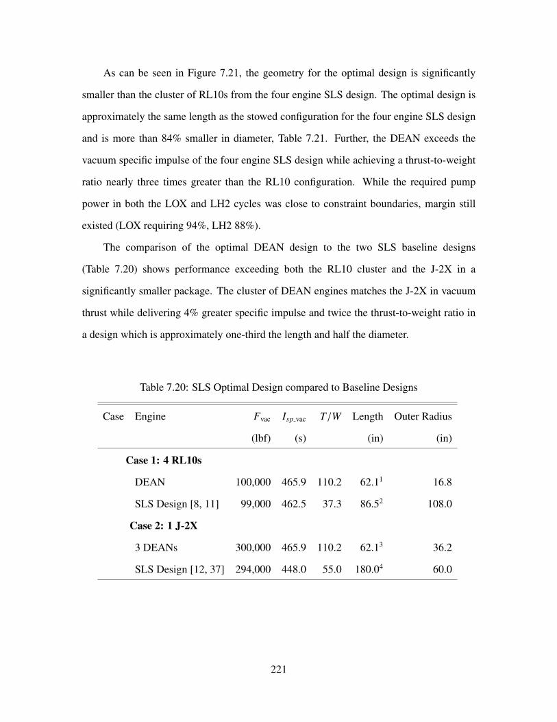
As can be seen in Figure 7.21, the geometry for the optimal design is significantly

smaller than the cluster of RL10s from the four engine SLS design. The optimal design is

approximately the same length as the stowed configuration for the four engine SLS design

and is more than 84% smaller in diameter, Table 7.21. Further, the DEAN exceeds the

vacuum specific impulse of the four engine SLS design while achieving a thrust-to-weight

ratio nearly three times greater than the RL10 configuration. While the required pump

power in both the LOX and LH2 cycles was close to constraint boundaries, margin still

existed (LOX requiring 94%, LH2 88%).

The comparison of the optimal DEAN design to the two SLS baseline designs

(Table 7.20) shows performance exceeding both the RL10 cluster and the J-2X in a

significantly smaller package. The cluster of DEAN engines matches the J-2X in vacuum

thrust while delivering 4% greater specific impulse and twice the thrust-to-weight ratio in

a design which is approximately one-third the length and half the diameter.

Table 7.20: SLS Optimal Design compared to Baseline Designs

Case Engine Fvac Isp vac T/W Length Outer Radius

(lbf) (s) (in) (in)

Case 1: 4 RL10s

DEAN 100,000 465.9 110.2 62.11 16.8

SLS Design [8, 11] 99,000 462.5 37.3 86.52 108.0

Case 2: 1 J-2X

3 DEANs 300,000 465.9 110.2 62.13 36.2

SLS Design [12, 37] 294,000 448.0 55.0 180.04 60.0

221

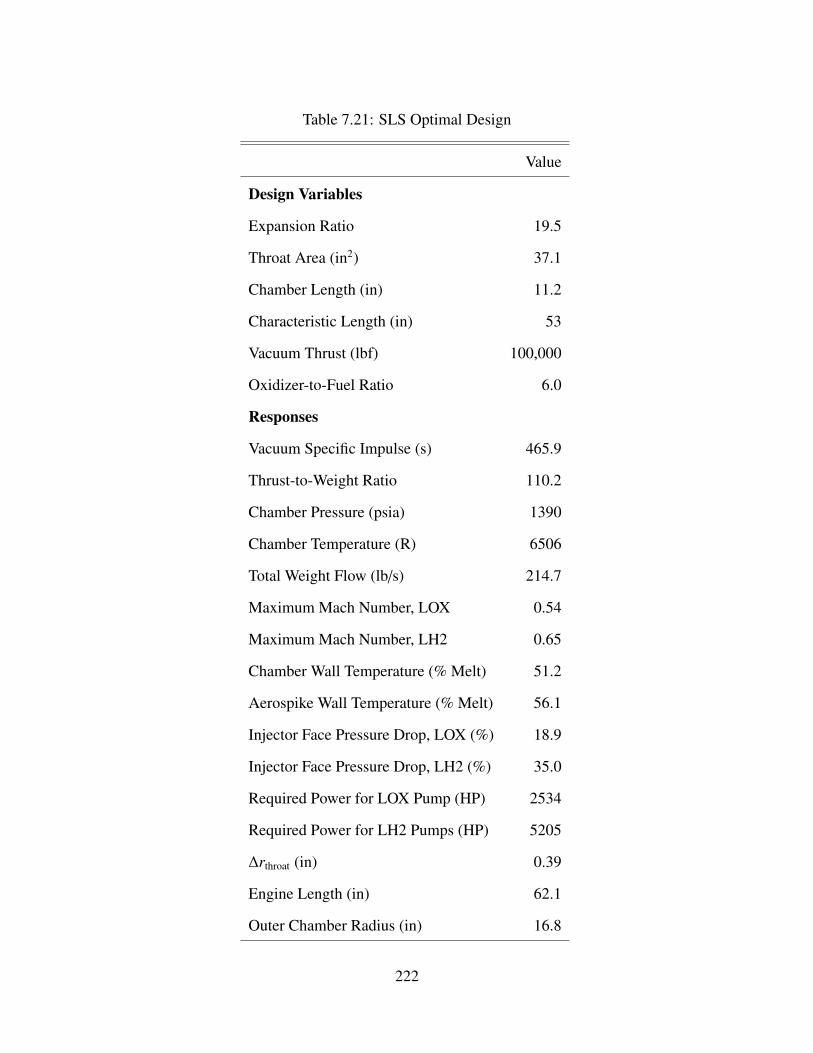
Table 7.21: SLS Optimal Design

Value

Design Variables







Responses



Chamber Pressure (psia) 1390

Chamber Temperature (R) 6506

Total Weight Flow (lb/s) 214.7

Maximum Mach Number, LOX 0.54

Maximum Mach Number, LH2 0.65

Chamber Wall Temperature (% Melt) 51.2

Aerospike Wall Temperature (% Melt) 56.1

Injector Face Pressure Drop, LOX (%) 18.9

Injector Face Pressure Drop, LH2 (%) 35.0

Required Power for LOX Pump (HP) 2534

Required Power for LH2 Pumps (HP) 5205

∆rthroat (in) 0.39



222

The LEO launch cost analysis from Section 7.4.2 was repeated for the two SLS

designs, substituting SLS design and performance data for the Atlas V and Delta IV

data. As with the IHPRPT/NGE DEAN, the launch cost analysis showed DEAN powered

upper stages offer increased payloads and in turn reduced launch costs. For the first SLS

design, using 4 RL10s providing 462.5 s of specific impulse, the DEAN provided 2540

lb of additional payload (1746 lb from engine weight savings and 794 lb from propellant

savings). This weight savings translated to a 1.2% reduction in launch costs. The second

SLS design, powered by a single J-2X engine providing 448.0 s of specific impulse, had a

more significant improvement. In this case, the DEAN upper stage increased the payload

by 8580 lb, with 2622 lb coming from engine weight savings and 5957 lb from propellant

savings. The related launch cost savings amount to a 3.7% reduction over the baseline SLS

design. As before, the results of this analysis are conservative estimates.

The results taken together support the conclusion that the DEAN’s performance,

compact size, and cost savings make it an excellent candidate for super-heavy lift launch

vehicles. The DEAN is not only an improvement over single expander cycle engines, it is

also competitive with gas generator cycle engines like the J-2X.

7.5 Conclusion

The results of this study support conclusions in two areas: critical constraints and

the viability of the DEAN architecture. The optimization studies revealed two critical

constraints on the DEAN architecture; injector face pressure drop and pump horsepower

requirements. For engines operating below the original design goal of 50,000 lbf thrust,

the LH2 pressure drop across the injector face frequently exceeded the constraint limit of

40%. For high thrust engines the limiting factor was the required pump power for both the

LOX pump (requiring 94% of the constraint value) and the LH2 pumps (requiring 88% of

the constraint value).

223

The DEAN is a viable and compelling alternative to traditional upper stage engines

across a wide range of missions. The DEAN offers significant improvements in thrust,

size, thrust-to-weight ratio, and launch costs over the RL10 for the IHPRPT/NGE mission.

The DEAN is also competitive for space plane missions, offering dramatic improvements

in specific impulse, size, and thrust-to-weight ratio over the AR2-3 and the RL10A-4. The

DEAN meets or exceeds the performance of SLS design options with more than twice the

thrust-to-weight, 4% greater specific impulse, and payload launch cost savings as high as

3.7%.

224

VIII. Conclusions and Recommendations

8.1 Research Objectives Answered

The goal of this research was to determine the viability of the DEAN architecture

by finding those missions and designs for which the DEAN’s performance and physically

compact packaging give it a competitive advantage over traditional upper stage engines.

Addressing this goal required answering the following questions.

• What are the operational limits of the DEAN architecture in terms of thrust and

specific impulse?

– The DEAN was optimized for designs ranging from 6600 lbf vacuum thrust for

the X-37 to 100,000 lbf vacuum thrust for the SLS. Trade studies conducted

during the SLS optimization study indicated the current model could not

reliably solve for DEAN designs above 100,000 lbf due to a number of physical

constraints.

• What are the limiting constraints of the DEAN architecture?

– The optimization studies revealed two critical constraints on the DEAN

architecture; injector face pressure drop and pump horsepower requirements.

For engines operating below the original design goal of 50,000 lbf thrust, the

LH2 pressure drop across the injector face frequently exceeded the constraint

limit of 40%. For high thrust engines the limiting factor was the required pump

power for both the LOX pump (requiring 94% of the constraint value) and the

LH2 pumps (requiring 88% of the constraint value).

• How does the DEAN compare to single expander cycle engines like the RL10 in

terms of specific impulse, thrust-to-weight ratio, and size?

225

– The DEAN exceeded the performance of the RL10. The DEAN generated up to

four times the thrust of the RL10 and exceeded the RL10B-2’s vacuum specific

impulse. The DEAN’s second cooling loop gave it more than four times the

pumping power of the RL10A-3 and more than twice the thrust-to-weight ratio

of the RL10A-4 and RL10B-2. The increased pumping power gave the DEAN

more than twice the chamber pressure of the RL10A-4 and RL10B-2 while

being less than half the length.

• What missions does the DEAN offer significant advantages over traditional upper

stage engines?

– The DEAN is a viable and compelling alternative to traditional upper stage

engines across a wide range of missions. The DEAN offers significant

improvements in thrust, size, thrust-to-weight ratio and launch costs over the

RL10 for the IHPRPT/NGE mission. The DEAN is also competitive for space

plane missions, offering dramatic improvements in specific impulse, size, and

thrust-to-weight ratio over the AR2-3 and the RL10A-4. The DEAN met or

exceeded the performance of SLS design options with more than twice the

thrust-to-weight, 4% greater specific impulse, and payload launch cost savings

as high as 3.7%.

8.2 Research Summary

Work at AFIT predating this research resulted in the development of an engine cycle

model of the DEAN for a single design. This cycle model was built in NPSS and calculated

the DEAN’s thrust, specific impulse, and state values for the propellants as they flowed

through the two expander cycles.

The first phase of this research built on the initial cycle model leading to the

development of a proof of concept parametric system model of the DEAN. The initial

226

system model used a direct parametrization of the NPSS cycle model favoring model

simplicity over traditional rocket engine design variables. This approach limited the

range of designs the model could explore. Specifically, this model had a low reliability

rating during trade studies varying radial geometry, crucial for studying the impact of the

expansion ratio. In spite of these limitations, parametric studies using this model resulted

in an improved design, demonstrating the utility of parametric modeling in rocket engine

design. The improved design was 25% shorter than the original design and reduced the

propellant weight flow by 14%.

The improved design showed the DEAN architecture offers significant performance

gains over single-expander cycle-based upper stage engines such as the RL10B-2. The first

phase design had a chamber pressure twice that of the RL10B-2 and twice the vacuum

thrust. Finally, this improved DEAN engine was 69% shorter than the RL10B-2, despite

its increased thrust.

The first phase results led to additional DEAN research efforts extending the DEAN

system model to include improved engine performance and estimate the engine weight.

These new analysis modules were incorporated into the second phase of this research. The

second topic converted the DEAN cycle model to a LOX/Methane engine to explore the

architecture’s capabilities with an alternate fuel.

The second phase of this research covered the development of a new system level

DEAN model integrating the lessons learned from the previous efforts to arrive at

a model with the necessary fidelity, flexibility, and reliability to address the overall

research questions. The development of this new model was driven by the limited trade

space size and low reliability of the prototype system model and later models built

from it. Improvements made in this new model included an updated parametrization,

model simplification, and calculating initial estimates for the NPSS solver. The updated

parametrization derived the engine geometry from traditional rocket engine parameters,

227

ensuring consistent designs and results. The model simplification replaced less reliable

external analysis modules with a modified NPSS rocket nozzle element to compute the

DEAN’s thrust from values available in the DEAN cycle model. Initial estimates for the

NPSS solver were calculated using a custom solver replacing previously static values with

design specific values.

The improvements in the new system level model had significant impacts on the

model’s flexibility and reliability. The trade studies using the new model showed it

supported a wide range of designs, including expansion ratios from 6.0 to 25.0. Trade

studies also indicated the new model’s reliability had improved significantly, with 98.7%

of the 1500 runs succeeding. The new system level DEAN model was used throughout the

remainder of this research.

The third phase of this research involved a detailed verification of the DEAN models

and architecture. The verification process began at the individual analysis level. The

source code for each engineering analysis was inspected and its methods and equations

were compared to engineering principles to ensure proper implementation. Additionally,

tests were run on key analysis modules to compare their calculations to expected results.

Once the individual analyses were verified, the DEAN architecture and system model were

tested using a series of parametric studies. These studies compared the DEAN’s responses

to rocket engineering theory and the RL10 family of expander cycle engines covering a

wide range of engine designs.

The verification studies confirmed the DEAN architecture is feasible and delivers

improved performance over single expander cycle engines in a compact package. The

studies also demonstrated the DEAN model is consistent with the scientific and engineering

principles of rocket propulsion. Finally the verification studies showed the DEAN

exceeds the performance of the RL10 for comparable thrust levels and proved the DEAN

architecture was ready for mission-specific comparisons to existing upper stage engines

228

The fourth phase of this research looked at the materials selection for the DEAN to

find a materials selection offering consistently low-weight engines across a wide range

of designs. This phase began with the development of an optimization process for the

design of the cooling channels in both expander cycles. This process was applied to a base

design for the materials selection study. The materials selection study then compared the

performance of the material options for each DEAN component over a variety of engine

designs.

The materials study yielded an updated materials selection covering a wide range

of engine designs. The materials study also confirmed the following findings from

previous research: the aerospike tip material selection has little influence on the engine’s

thrust-to-weight ratio, the chamber cooling jacket should be manufactured from silicon

carbide, the LOX plumbing should be manufactured from INCONEL 718, and the LH2

plumbing should be manufactured from INCOLOY 909. The material study also found

updated material selections for the aerospike cooling jacket (silicon carbide), chamber

structural jacket (INCONEL 718), and the aerospike structural jacket (INCOLOY 909)

which produced low weight engines across a wide range of designs compared to previous

material selections.

Finally, the fifth phase of this research covered a series of optimization studies of

the DEAN for the IHPRPT/NGE, X-37, and SLS missions and compared the DEAN’s

performance and size to traditional upper stage engines. This phase began by defining

the top level design variables, preassigned parameters, and constraints for the DEAN

optimization studies. A sensitivity study over the design variables identified key response

variables and relationships between the design variables and key response variables. These

results were used to develop an optimization process for the DEAN architecture.

The optimization process was then applied to the IHPRPT/NGE, X-37, and SLS

missions. The DEAN outperformed traditional upper stage engines for all three missions.

229

For the NGE program, the optimized design delivers 35,000 lbf of vacuum thrust and 469.4

seconds of vacuum specific impulse with a thrust-to-weight ratio of 127.2 in an engine one

quarter the size of a comparable RL10. For the X-37 mission, the optimized design operates

at 6,600 lbf of vacuum thrust and has a vacuum specific impulse of 457.2 seconds with a

thrust-to-weight ratio of 107.5. For the SLS, the optimized design produces a vacuum thrust

of 100,000 lbf and a vacuum specific impulse of 465.9 seconds with a thrust-to-weight

ratio of 110.2. When configured in a cluster of three engines, the DEAN matches the J2-X

vacuum thrust with a 4% increase in specific impulse while more than doubling the J2-X’s

thrust-to-weight ratio. Payload launch cost savings to Low Earth Orbit for DEAN powered

upper stages ranged from 1.1% to 4.75% depending on mission.

8.3 Research Contributions

1. A method for parametrically modeling rocket engines in NPSS was demonstrated

including calculation of initial estimates for key parameters in the NPSS model

and calculation of fluid Mach numbers in the cooling channels. The method

mapped traditional rocket engine parameters to the geometry and other engine design

parameters in the NPSS model. The initial estimates for the specific impulse and

pump pressure ratios were calculated using a custom external solver. Mach numbers

were calculated using Kriging Response Surface Models (RSMs) configured with

data from National Institute of Standards and Technology. This work is covered

in Chapter 3 (published in the AIAA Journal of Spacecraft and Rockets [27]) and

Chapter 4.

2. The DEAN architecture was verified through a series of six parametric studies. These

parametric studies covered relationships driven by the top level design variables:

thrust, throat area, expansion ratio, oxidizer-to-fuel ratio, chamber length, and

characteristic length. Responses tested with the trade studies included chamber

230

pressure, propellant weight flow, specific impulse, and engine weight. Each trade

study varied the design variable under test plus an additional design variable to ensure

the results covered a wide range of designs and not a narrow band of designs. The

results from these trade studies verified the DEAN architecture conforms to rocket

engine theory and exceeds the RL10’s performance. This work is covered in Chapter

5 (submitted to the AIAA Journal of Propulsion and Power).

3. The materials selection proposed in previous research was refined to support a wide

variety of missions and engine designs. Using optimized cooling channel designs for

both expander cycles, a series of trade studies were run to find material selections

yielding consistently low engine weight. These trade studies varied engine designs

and material selections to give results spanning a wide range of engine designs. The

results confirmed a number of previous findings and improved upon others. This

work is covered in Chapter 6.

4. An optimization process for DEAN engines using the DEAN system level model

was developed and demonstrated. The optimization problem solved by this process

is a multi-objective problem seeking to maximize the DEAN’s specific impulse and

thrust-to-weight ratio. This process used the results of a sensitivity analysis to

efficiently scope the optimization problem before solving it using a genetic algorithm

to generate a Pareto front of specific impulse variation with thrust-to-weight ratio.

The process was applied to the mission requirements for the IHPRPT/NGE programs,

the X-37 space plane, and two upper stage configurations of the SLS. This work is

covered in Chapter 7 (submitted to the AIAA Journal of Spacecraft and Rockets).

5. Optimal DEAN engine designs were found for three IHPRPT/NGE cases, the X-37

space plane, and two upper stage configurations of the SLS. The results of applying

the optimization process above to these three missions show the DEAN is a viable

231

and compelling alternative to traditional upper stage engines across a wide range of

missions. Across all three missions, the DEAN meets or exceeds traditional upper

stage engines in thrust and specific impulse while offering improved size and thrust-

to-weight ratios. This work is covered in Chapter 7 (submitted to the AIAA Journal

of Spacecraft and Rockets).

8.4 Recommendations for Future Research

The recommendations in this section fall into two categories: extending current results

and fifth generation DEAN research. The extending current results recommendations cover

work building on results from this research without requiring additional simulation runs in

the fourth generation DEAN model. The fifth generation DEAN research recommendations

cover updates and additional parametric studies for the DEAN system model.

8.4.1 Extending Current Results.

8.4.1.1 Update Turbopump Design Studies.

During the first generation DEAN research Arguello and Strain designed the

turbopumps for the LH2 and LOX cycles respectively. Their work verified the results from

the cycle model and the first generation DEAN design [25, 26]. Repeating these design

studies for the designs presented in Chapter 7 would further verify the fourth generation

DEAN model and the optimized designs for the IHPRTP/NGE, X-37, and SLS DEAN

engines. Given the number of designs to be considered (two turbopumps for five designs

totaling ten turbopump designs), parametric modeling techniques should be explored for

turbopump design software, Pumpal and RITAL, before running the individual design

studies.

8.4.1.2 Update the Methane DEAN Study.

The Methane DEAN research suffered from similar challenges to those of the second

and third generation DEAN research studies. The fourth generation DEAN system

model’s improvements successfully addressed those challenges for the LOX/LH2 DEAN

232

architecture. It is possible these changes could improve the Methane DEAN model’s

reliability and trade space size as well. A second generation Methane DEAN model should

be built based on the lessons learned in the fourth generation DEAN model to determine if

its improvements can yield improved results for the design of the Methane DEAN.

8.4.2 Fifth Generation DEAN Research.

8.4.2.1 Recommended Model Updates.

The fourth generation DEAN model was a major step forward in simulating the

DEAN. However, it represents the limits of what can be done with the current DEAN cycle

model. Future DEAN modeling should begin with a clean implementation of the DEAN

cycle model in NPSS. This new implementation can address a number of outstanding

concerns about the current cycle model. First and foremost, this clean implementation can

be built from the ground up to support parametric design. Post research analysis indicated

the current cycle model still contains a small number of fixed geometry elements that should

be sized to match the current design. Additional post research analysis indicated there may

be modeling elements in the cycle model needing their thermal connections verified. These

thermal connections may be contributing to the high pressure drops across the injector face.

Updating the cycle model implementation would also facilitate moving from NPSS v1.6.5

to the current commercial release.

To improve simulation execution time, the pre and post processing steps from the

DEAN system model should be incorporated into the NPSS source code, making the NPSS

model the DEAN system model, and reserving ModelCenter for integration with outside

tools and automation of the DEAN model. Finally, unit tests should be developed for the

individual analysis modules in the DEAN model to further verify their implementations

and provide a framework for supporting future upgrades to the DEAN models.

233

8.4.2.2 Additional Design Studies.

The anticipated improvements in the fifth generation DEAN model make it suitable

for additional DEAN design studies. Possible design studies include revisiting the third

generation DEAN research into truncated nozzles, further improving the cooling channel

design and optimization processes, investigating alternative materials for the cooling

jackets, and investigating the marginal designs from the optimization studies in Chapter

7. While Chapter 6 confirmed the aerospike tip does not have a significant impact on

the DEAN’s thrust-to-weight ratio, the tip does have a significant impact on the overall

engine length and in turn the length of the interstage hardware impacting stage weight.

With the wall temperatures being one of the key constraints in the DEAN architecture,

continuing to study and improve the cooling channel designs and material selections for

the cooling jackets can only improve the results of DEAN research. Finally, the proposed

improvements in the fifth generation DEAN model should address some of the causes of

the high pressure drops across the injector face, possibly bringing the marginal designs

from Chapter 7 back into compliance with the constraint boundaries.

8.4.2.3 Detailed Comparison of DEAN to RL10 and J-2X Using an Upper

Stage Model.

The fifth generation DEAN model should be used to perform a detailed comparison

between the DEAN and traditional upper stage engines using an upper stage model. The

upper stage model should be parametric and include design variables to vary payload

weight and orbit, propulsion system (including the DEAN, RL10, and J-2X), and controls

for the sizing method (size stage for payload or size payload for stage). The upper stage

model should then be used to compare the DEAN’s performance to the RL10 and J-2X for

a variety of missions and payloads. Potential figures of merit include total stage weight

for a given payload weight, available payload weight for a given stage weight, and percent

growth of stage weight per percent growth in payload weight.

234

Appendix A: Verification and Validation of the Fourth Generation DEAN Model

A.1 Introduction

This appendix covers the verification and validation of the individual analysis modules

making up the fourth generation DEAN system model, shown in Figure A.1 and Table A.1.

The organization of the appendix follows the structure of the model, beginning with the

Design Variables analyses and continuing through the Constraints. Each section covers the

purpose, assumptions, underlying engineering models, and implementation for the analysis

modules under consideration. Verification is carried out through source code inspection

and isolated analysis level testing. The source code inspection uses line by line review of

the analysis source file and comparing the source code to the engineering principles used

in the analysis. Validation is conducted by comparing the results of the analysis module to

its purpose.

Figure A.1: Fourth Generation DEAN Model

235

Table A.1: Fourth Generation DEAN Model Components







cycles








thicknesses


nesses and T/W




the injector face

The fourth generation DEAN model is built using ModelCenter’s process modeling

feature. Process modeling gives model developers access to new model elements and

alters how existing elements affect the execution of the model. In models built using

236

these features, often called process models, the analyses are run from left to right or top

to bottom depending on the model’s layout, and may include various control structures.

The DEAN system level model uses several of these structures including sequences, for-

each loops, parallel branches, and if branches. Sequences, shown in Figure A.2(a),

provide a means of visually organizing analysis components in ModelCenter and for

storing system level variables. Analyses in a sequence execute in the same order as the

containing model. For-each loops, shown in Figure A.2(b), take scalar analyses and run

them iteratively over arrays of inputs while capturing the results in output arrays turning

scalar analyses into vector analyses. Parallel branches, shown in Figure A.2(c), organize

analyses which are not interdependent in a parallel structure. Analyses which support

parallel execution run simultaneously when organized under parallel branches. Finally, if

branches, (Figure A.2(d)) provide a means of controlling the execution of analyses. During

model execution, if branches select one or more paths to execute based on the specified

branch condition. Using if branches, model developers can selectively run analyses to

switch model fidelity, model required work flows, or implement model level exception

handling [67].

In addition to process modeling features, the DEAN model uses a specialized looping

structure and a built-in geometry component. The looping structure is the Converger, shown

in Figure A.3. The Converger is a ModelCenter component which implements a fixed-point

iteration solver to find designs where a calculated value matches the guessed value for one

or more parameters. The Converger creates a loop when used in process models [67].

The built-in geometry component used in the DEAN system level model is the

GenericSOR (Surface of Revolution) component. The GenericSOR, shown in Figure A.4,

renders a surface of revolution in ModelCenter’s geometry views, such as the embedded

geometry of a cone shown in Figure A.4. The revolved surface is defined by a string input

variable containing a list of points defining the curve to be revolved around the x-axis [67].

237

(a) Sequence Component (b) For-Each Loop

(c) Parallel Branch (d) If Branch

Figure A.2: ModelCenter Process Components

In the DEAN model, GenericSOR components are used to render the primary elements of

the DEAN including the chamber and the aerospike.

238

Figure A.3: ModelCenter Converger

Figure A.4: ModelCenter Surface of Revolution Component

239

A.2 Preprocessing Step: Design Variables

The preprocessing steps in the DEAN system model are implemented by the Design

Variables sequence, shown in Figure A.5. The first two analyses, running in a parallel

branch, manage the material selections for the aerospike and the designs for the cooling

channels. The final component is an embedded ModelCenter sub-model implementing

a custom solver process to find the initial estimates for design variables relating to the

pressure profiles in the two expander cycles.

Figure A.5: DEAN Preprocessing Components

In addition to the analysis modules, the Design Variables sequence contains the

declarations for the DEAN system level design variables. These design variables fall into

three categories: engine design variables (Table A.2), modeling assumptions (Table A.3),

and cooling channel design variables (Table A.4).

240

Table A.2: DEAN Engine Design Variables


Expansion Ratio Ratio of the exit area (Ae) to the throat area (At)

Throat Area (in2) Area of the nozzle at the throat

Chamber Length (in) Length of the chamber, runs from the back of the

engine to the throat

Characteristic Length (in) Ratio of the chamber volume (Vc) to the throat area

(At)

Vacuum Thrust (lbf) Specified thrust to be produced by the engine

Oxidizer-to-Fuel Ratio Ratio between the propellants

Table A.3: DEAN Modeling Assumption Design Variables


Ambient Pressure Decision Controls whether aerospike geometry is modeled for

design or operational altitude

Operational Pressure (psia) Ambient pressure (for vacuum, assumes 0.001 psia)

Cooling Geometry Option Controls whether the cooling channels include a

separate cover or if the structural jacket is the cover

Percent Weight of Hardware Percent of the overall engine mass accounted for by

miscellaneous hardware

Cowl Length (% Spike Radius) Length of the engine cowl (normalized to aerospike

radius at the throat)

Factor of Safety Factor of safety for structural sizing modules

Material Strength Option Controls whether structural sizing modules use ulti-

mate or yield strength for stress tests

LOX Tank Pressure (psia) Tank pressure for the LOX tank

LH2 Tank Pressure (psia) Tank pressure for the LH2 tank

241

Table A.4: DEAN Cooling Channel Design Variables


Chamber Throat AR Aspect ratio of the chamber cooling channels at the

throat

Chamber Stations Adjustment Controls how the aspect ratio of chamber cooling

channels vary over the length of the engine

Chamber Station 5 Adjustment Controls the aspect ratio of the chamber cooling

channels at station 5

Chamber Cooling Channels Ratio Ratio of the number of chamber cooling channels to

the chamber circumference at the throat

Nozzle Throat AR Aspect ratio of the aerospike cooling channels at the

throat

Nozzle Station 1 Adjustment Controls the aspect ratio of the aerospike cooling

channels at station 1

Nozzle Stations Spike Adjustment Controls how the aspect ratio of aerospike cooling

channels vary over the length of the engine

Aerospike Cooling Channels Ratio Ratio of the number of aerospike cooling channels to

the aerospike circumference at the throat

242

A.2.1 Spike Materials.

The purpose of the Spike Materials component is to manage the material selections

for the aerospike components during trade studies, allowing for parametric studies over

material selections for multiple engine components when they use the same material. Each

material selection is coded as an integer based on the values used in the Material Properties

component. The source code for the Spike Materials component is shown in Listing A.1.

It is structured as a series of cases. The three cases are: the aerospike is made of a single

material (lines 2-7), the structural jacket and tip are the same material (lines 8-13), and each

component is controlled individually (lines 14-18).

Listing A.1: Spike Materials Source Code

1 function run() {2 if (Unified_Spike.value) {3 Spike_Cool_Mat.value = All_Spike_Mat.value;4 // shift over 1 for SJ material5 SJSpike_Mat.value = All_Spike_Mat.value + 1;6 Spike_Tip_Mat.value = All_Spike_Mat.value;7 }8 else if (UnifiedSJandTip.value) {9 Spike_Cool_Mat.value = Spike_Cool_Mat_In.value;

10 SJSpike_Mat.value = SJSpike_Mat_In.value;11 // shift back by 1 for tip material12 Spike_Tip_Mat.value = SJSpike_Mat_In.value - 1;13 }14 else {15 Spike_Cool_Mat.value = Spike_Cool_Mat_In.value;16 SJSpike_Mat.value = SJSpike_Mat_In.value;17 Spike_Tip_Mat.value = Spike_Tip_Mat_In.value;18 }19 }

Inspection of the source code showed the component was implemented correctly.

Consider the first case, where the aerospike is made of a single material. Line 2 determines

if this is the currently selected case by testing the boolean variable Unified Spike. Then,

lines 3-6 assign the unified material selection (All Spike Mat) to each of the three aerospike

components: the cooling jacket, the structural jacket, and the tip. The material coding for

the structural jacket is one greater than the cooling jacket and the tip, so the structural jacket

is assigned a value one greater than the unified material code. A similar process is used

243

for the other two cases. As is shown from this inspection, the Spike Materials component

correctly manages the materials selection for the aerospike components for all three use

cases, fulfilling its purpose.

A.2.2 Cooling Channels Design.

The purpose of the Cooling Channels Design component is to determine physical

design parameters of the chamber and aerospike cooling channels. The physical design

parameters for the cooling channels include the number of cooling channels and the

scheduling of the cooling channels’ aspect ratios along the length of the engine. The

component was verified through inspection of its source code.

The number of cooling channels in each of the expander cycles is proportional to the

circumference of the element being cooled (either the chamber or the aerospike), and is

constrained by the minimum channel spacing of 0.02 inches. The Number of Channels

component calculates the circumferences for both the chamber and the aerospike, then

applies scaling factors to determine the number of channels in each expander cycle.

The aspect ratios for the cooling channels are based upon Martin’s approach to

designing the cooling channels. In the first generation DEAN research, Martin used varying

aspect ratios along the length of the cooling channels to balance the cooling needs with the

maximum Mach number constraints. In both cooling jackets, Martin selected low aspect

ratios (shorter channels, smaller cross-sectional area) at the throat to increase the cooling

rate and higher aspect ratios (taller channels, larger cross-sectional areas) at the end of

the cooling jacket to maintain a velocity below the maximum allowable Mach number.

The smaller cross-sectional area in the low aspect ratio regions increases the fluid velocity

and in turn the power required to pump the fluid. This increase in required pump power

drives the solver in the cycle model toward designs yielding more power from the turbine

by increasing the amount of heat extracted from cooling the engine, effectively increasing

the cooling rate in those regions. The larger cross-sectional areas in the high aspect ratio

244

regions reduce the velocity of the fluid and account for the decrease in density (increase

in volume) caused by heating the fluid. Combined, these two effects ensure the fluid stays

below its Mach number limit, preventing catastrophic failure of the engine [2]. In the

Cooling Channels Design component, the throat station is used as the specified aspect ratio

and scaling multipliers are used to control how the aspect ratios change along the length of

the engine.

Listing A.2 contains the source code for the Cooling Channels Design component.

Line 2 calculates the outer throat radius, which is also the radius of the exit area.

Rearranging the definition of expansion ratio, see Equation (A.1), and combining it with the

relationship between the area of a circle and its radius gives Equation (A.2), implemented

in Line 2. Line 3 calculates the inner throat radius from the throat area. The DEAN throat is

the annulus defined by the inner and outer throat radii which correspond to the nozzle and

chamber structures at the throat. Equation (A.3) is the equation for the area of an annulus.

Solving this equation for the inner radius yields Equation (A.4) and is implemented by Line

3. Lines 5 and 6 compute the number of channels by multiplying the circumference (2rπ)

of the chamber and aerospike by their respective scaling factors and rounding the results to

yield integer values.

The remainder of Listing A.2 computes the aspect ratios. Lines 8-25 calculate the

aspect ratios for the chamber cooling channels. The for loop defined in Line 8 iterates over

the six stations in the chamber. The if statements within the loop select the appropriate

scaling factor for each station: no scaling factor for the throat on Lines 9 and 10, the station

5 scaling factor on Lines 11-13, and the default scaling factor on Lines 14-24. In Martin’s

scheduling for the chamber aspect ratios, station 1 has an approximately 25% higher aspect

ratio than the preceding stations. This adjustment is applied in Line 17 unless the scaling

factor equals 1.0. In the case of the scaling factor equaling 1.0, the component applies

245

a constant aspect ratio along the entire length of the engine. Lines 18-20 implement the

branch to handle this case for station 1. Finally, Lines 22-24 cover the remaining stations.

Similarly, Lines 27-47 calculate the aspect ratios for the nozzle cooling channels. The

for loop defined in Line 27 iterates over the eight stations in the nozzle. Using Martin’s

scheduling approach, the throat is not scaled (Lines 28-29), the stations immediately before

and after the throat are scaled up 20% unless the aspect ratios are constant (Lines 30-35),

the final station is scaled by the spike scaling factor (Lines 36-38), the first two stations

are scaled by the station 1 scaling factor (Lines 39-41), and the remaining stations linearly

adjust their aspect ratios from station 2 to station 5 (Lines 42-46). The linear transition is

implemented by computing and applying a step increment.

Listing A.2: Cooling Channels Design Source Code

1 function run() {2 var r_to = Math.sqrt(ExpansionRatio.value * ThroatArea.value / Math.PI);3 var r_ti = Math.sqrt(Math.pow(r_to,2) - (ThroatArea.value / Math.PI));4

5 ChamberN.value = Math.round(2 * r_to * Math.PI * ChamberNRatio.value);6 NozzleN.value = Math.round(2 * r_ti* Math.PI * NozzleNRatio.value);7

8 for (i = 0; i < ChamberStationsAR.length; i++) {9 if (i == 5)

10 ChamberStationsAR.value(i) = ChamberThroatAR.value;11 else if (i == 4)12 ChamberStationsAR.value(i) = ChamberThroatAR.value *13 ChamberStation5Adjustment.value;14 else if (i == 0) {15 if (ChamberStationsAdjustment.value != 1.0) // Matching Martin16 ChamberStationsAR.value(i) = ChamberThroatAR.value *17 ChamberStationsAdjustment.value * 1.25;18 else // if adjustment == 1.0, no additional scaling19 ChamberStationsAR.value(i) = ChamberThroatAR.value *20 ChamberStationsAdjustment.value;21 }22 else23 ChamberStationsAR.value(i) = ChamberThroatAR.value *24 ChamberStationsAdjustment.value;25 }26

27 for (i = 0; i < NozzleStationsAR.length; i++) {28 if (i == 5)29 NozzleStationsAR.value(i) = NozzleThroatAR.value;30 else if ((i == 6) || (i == 4)) {31 if (NozzleStationsSpikeAdjustment.value != 1.0)32 NozzleStationsAR.value(i) = NozzleThroatAR.value * 1.2;33 else // if spike adjustment == 1, no additional scaling34 NozzleStationsAR.value(i) = NozzleThroatAR.value;35 }

246

36 else if (i == 7)37 NozzleStationsAR.value(i) = NozzleThroatAR.value *38 NozzleStationsSpikeAdjustment.value;39 else if ((i == 0) || (i == 1))40 NozzleStationsAR.value(i) = NozzleThroatAR.value *41 NozzleStation1Adjustment.value;42 else {43 var step = (NozzleStationsAR.value(0) - (NozzleThroatAR.value +44 NozzleThroatAR.value * NozzleStationsSpikeAdjustment.value)/2)/3;45 NozzleStationsAR.value(i) = NozzleStationsAR.value(i-1) - step;46 }47 }48 }

ε = Ae/At (A.1)

rto =√ε ∗ At/π (A.2)

A = π(r2o − r2

i ) (A.3)

ri =

√r2

o − A/π (A.4)

Calculating the required number of cooling channels based on changes to the radial

size and determining the cooling channel aspect ratios for the DEAN is essential to making

the DEAN model capable of operating over a wider range of design points. As the

above inspection shows, the Cooling Channels Design component correctly calculates these

values, validating this component.

A.2.3 Pressure Profile Converger.

The purpose of the Pressure Profile Converger, implemented as an embedded

ModelCenter sub-model and shown in Figure A.6, is to determine the initial estimates

for the vacuum specific impulse and the pressure ratios of the LOX and LH2 pumps. These

four values drive the calculations for the estimated pressure profiles in the two expander

cycles, and have a significant impact on the reliability and the results of the DEAN cycle

247

model. Prior to the inclusion of the Pressure Profile Converger, the DEAN system level

model used a static set of estimates for these variables, despite their dependance on design

variables such as thrust and expansion ratio. The Pressure Profile Converger sub-model

includes a custom solver, a copy of the DEAN cycle model, and an error calculation

analysis to determine the quality of the estimated pressure profiles. This component was

verified through inspection and testing.

Figure A.6: Pressure Profile Converger Components

The custom solver iteratively calls the other components to determine the best values

for the four required initial estimates. First, the solver calls the DEAN cycle model,

stepping through values for the specific impulse and pump pressure ratios until the DEAN

analysis runs to completion and returns a calculated value for the specific impulse. The

DEAN cycle model is very sensitive to the pump pressure ratios and will often fail when

given poor estimates. However, the specific impulse calculation is not strongly affected by

these variables. Therefore, the first successful run of the DEAN cycle model is sufficient to

yield a high quality estimate for the specific impulse.

248

The custom solver then uses the estimated specific impulse for the remaining iterations

carried out in two loops. The first loop solves for the LOX pump pressure ratio by finding

a series of working pressure ratios and selecting the one with the lowest root mean square

error across the entire LOX cycle. The second loops uses a similar approach to solve for

the pressure ratio of the first LH2 pump. Note, the solver always assumes the second LH2

pump has a pressure ratio of 2.0 based on current design assumptions for the DEAN.

Listing A.3 contains the source code for the custom solver in the Pressure Profile

Converger. Lines 4-11 initialize the design variable estimates and internal arrays used to

track intermediate results in the solver. Note, the estimated specific impulse (TargetIsp)

is initialized to −1.0 s, making the success condition for the specific impulse loop any

specific impulse greater than zero. Lines 14-18 solve for the estimated specific impulse by

iteratively calling the findTargetIsp function (Listing A.4). To save iterations, the for loop

declared in Line 14 uses a series of decreasing step sizes (the value n) in the findTargeIsp

function. Lines 16-17 contain the success criteria, testing for positive values of specific

impulse and breaking out of the for loop when one is found. Lines 20-23 conclude the

estimation process for the specific impulse by testing for success after the specific impulse

iteration, throwing an error if the for loop was unsuccessful and setting the specific impulse

value used in later iterations to the updated estimate otherwise.

Lines 26-46 solve for the estimated value of the LOX pump pressure ratio. Line 26

calls the setGuessLowerValues function (Listing A.5) to initialize the limits of the for loop

used to solve for the LOX pump pressure ratio (Lines 28-29). Lines 30-31 set the pressure

ratios used in the cycle model for the current iteration. The try-catch block in Lines 32-42

stores the current estimate for the LOX pump pressure ratio (Line 33) and executes the

DEAN cycle model and the root mean square error calculation component (Line 34). The

DEAN cycle model generates a ModelCenter error when it fails to find a solution for the

current design, using the try-catch block enables the custom solver to trap the ModelCenter

249

error and continue executing the current iteration loop (Lines 40-41). Lines 35-38 break out

of the iteration loop when the current results yield an error value greater than the previous

iteration. Otherwise the loop is continued. This early exit is included to save computation

time by eliminating unnecessary iterations. Solving for the estimated LOX pump pressure

ratio concludes with Lines 45-46 which call the findBestPR function to iterate through the

results and find the pressure ratio with the lowest root mean square error and setting the

DEAN cycle model and the Pressure Profile Converger results to this value.

A similar process is applied to find the LH2 pump 1 pressure ratio estimate in Lines

49-68. Finally, Line 71 executes the DEAN cycle model and the root mean square error

calculation one final time to compute and record the root mean square error for the final

estimates found by the Pressure Profile Converger.

Listing A.3: Pressure Profile Converger Source Code

1 void function run() {2

3 // initialize key vars4 TargetIsp.value = -1;5 LH2Pump2PRGuess.value = LH2Pump2PRGuessDefault;6 PRdes_Pump2F.value = LH2Pump2PRGuessDefault;7

8 var LOXPumpPRGuessValues = new Array();9 var LOX_RMSEValues = new Array();

10 var LH2Pump1PRGuessValues = new Array();11 var LH2_RMSEValues = new Array();12

13 // solve for TargetIsp14 for (var n = 4; n >= 1; n = n/2) {15 findTargetIsp(n);16 if (TargetIsp.value > 0)17 break;18 }19

20 if (TargetIsp.value < 0)21 throw "Unable to find TargetIsp";22 else23 IspGuess.value = TargetIsp.value;24

25 // solve for LOX Pump PR26 setGuessLowerValues();27 var iLOX = 0;28 for (LOXpr = LOXPumpPRGuessLower; LOXpr <= LOXPumpPRGuessUpper;29 LOXpr += PumpPRGuessStep) {30 LOXPumpPRGuess.value = LOXpr;31 LH2Pump1PRGuess.value = LH2pr;32 try {33 LOXPumpPRGuessValues[iLOX] = LOXpr;

250

34 LOX_RMSEValues[iLOX] = LOX_RMSE.value;35 if ((iLOX > 0) && (LOX_RMSEValues[iLOX-1] < LOX_RMSEValues[iLOX]))36 break;37 else38 iLOX++;39 }40 catch (err) {41 // continue42 }43 }44

45 PRdes_PumpO.value = findBestPR(LOXPumpPRGuessValues, LOX_RMSEValues);46 LOXPumpPRGuess.value = PRdes_PumpO.value;47

48 // solve for LH2 Pump 1 PR49 setGuessLowerValues();50 var iLH2 = 0;51 for (LH2pr = LH2Pump1PRGuessLower; LH2pr <= LH2Pump1PRGuessUpper;52 LH2pr += PumpPRGuessStep) {53 LH2Pump1PRGuess.value = LH2pr;54 try {55 LH2Pump1PRGuessValues[iLH2] = LH2pr;56 LH2_RMSEValues[iLH2] = LH2_RMSE.value;57 if ((iLH2 > 0) && (LH2_RMSEValues[iLH2-1] < LH2_RMSEValues[iLH2]))58 break;59 else60 iLH2++;61 }62 catch (err) {63 // continue64 }65 }66

67 PRdes_Pump1F.value = findBestPR(LH2Pump1PRGuessValues, LH2_RMSEValues);68 LH2Pump1PRGuess.value = PRdes_Pump1F.value;69

70 // run the analysis one more time with final values to get RMSEs71 var LH2_RMSE_value = LH2_RMSE.value;72 }

Listing A.4 contains the source code for the findTargetIsp function. This function

iteratively runs the DEAN cycle model to find an estimate for the specific impulse and is

driven by the for loop declared in Line 3. This for loop iterates over a series of estimates

for the specific impulse until the DEAN cycle model returns a final estimate for the specific

impulse. For each estimated specific impulse, the DEAN cycle model is set to use the

current estimate (Line 4), initialize the limits for the pressure ratios used in the nested for

loops below by calling the setGuessLowerValues function (Line 5), and then uses a pair of

nested for loops to iteratively call the DEAN cycle model with a series of pressure ratio

estimates until the cycle model returns a valid specific impulse estimate. The two for loops

251

(Lines 6-7 and Lined 9-10) use the stepN argument to modify the step size, with larger step

sizes giving fewer iterations. The try-catch block in Lines 12-18 captures ModelCenter

errors from failed runs of the cycle model and exits the function using the return statement

(Line 14) when the estimated specific impulse is found.

Listing A.4: Find Taget Isp Function Source Code

1 function findTargetIsp(stepN) {2 // looking for first successful run to get target isp3 for (var isp = IspGuessLower; isp <= IspGuessUpper; isp += IspGuessStep) {4 IspGuess.value = isp;5 setGuessLowerValues();6 for (LH2pr = LH2Pump1PRGuessLower; LH2pr <= LH2Pump1PRGuessUpper;7 LH2pr += (stepN*PumpPRGuessStep)) {8 LH2Pump1PRGuess.value = LH2pr;9 for (LOXpr = LOXPumpPRGuessLower; LOXpr <= LOXPumpPRGuessUpper;

10 LOXpr += (stepN*PumpPRGuessStep)) {11 LOXPumpPRGuess.value = LOXpr;12 try {13 TargetIsp.value = IspResult.value;14 return;15 }16 catch(err) {17 // continue18 }19 }20 }21 }22 }

Listing A.5 contains the source code for the setGuessLowerValues function. Orig-

inally designed to calculate the lower limits for the pump pressure ratio estimates, this

function was later modified to compute both the upper and lower limits. Lines 2-3 break

up the calculation of the estimated chamber pressure into two steps. The chamber pressure

can be found from the characteristic velocity, thrust, specific impulse, and throat area as

shown in Equation (A.5). Line 2 calculates the weight flow, Equation (A.6), for use in

the chamber pressure calculation in Line 3. Substituting the definition for the weight flow

from Equation (A.6) into the chamber pressure calculation gives Equation (A.7), which is

implemented in Line 3.

The remaining lines use the estimated chamber pressure to compute the upper and

lower limits for the pressure ratios. The pressure ratios are computed from the ratio of the

252

of the chamber pressure to the pressure coming into the pump times the estimated pressure

losses in the plumbing. The upper limits are set to 250% of this ratio and the lower limits

are set to 175% of this ratio.

Listing A.5: Set Guess Lower Values Function Source Code

1 function setGuessLowerValues() {2 var wdot = Thrust.value / IspGuess.value;3 var P_c_guess = wdot * c_star / (ThroatArea.value * g0);4 LH2Pump1PRGuessLower = Math.floor((1.75 * P_c_guess) /5 (P_TankH * plumbingLosses) / LH2Pump2PRGuessDefault);6 LH2Pump1PRGuessUpper = Math.floor((2.5 * P_c_guess) /7 (P_TankH * plumbingLosses) / LH2Pump2PRGuessDefault);8 LOXPumpPRGuessLower = Math.floor((1.75 * P_c_guess) / (P_TankO * plumbingLosses));9 LOXPumpPRGuessUpper = Math.floor((2.5 * P_c_guess) / (P_TankO * plumbingLosses));

10 }

pc =c∗F

IspAtg0(A.5)

w =FIsp

(A.6)

pc =c∗wAtg0

(A.7)

The simulation results and reliability of the DEAN system model before and after

integrating the Pressure Profile Converger demonstrated it is functioning correctly. Before

integrating the Pressure Profile Converger, initial surveys of the DEAN trade space

indicated the pressures in the cooling channels were inversely proportional to the thrust

and directly proportional to the expansion ratio. A design of experiments over the thrust,

expansion ratio, and throat area was run to test these results (Table A.5).

The results of cooling channel pressure study are shown in Figure A.7. In the figure,

the horizontal axis is the expansion ratio, the vertical axis is the pressure in the LOX cooling

channel at the throat, and the axis running into the page is the throat area. Additionally,

253

Table A.5: Design Variables for Cooling Channel Pressure Study





the color of the data points represents the thrust level, with blue points representing thrust

levels of 20,000 lbf at the low end, and red points representing thrust levels of 50,000 lbf at

the high end. These results support the conclusions from the initial surveys of the DEAN

trade space. For a given thrust level, indicated by points of a single color, the pressure in

the LOX cooling channel increased with increasing expansion ratio. Further, the highest

pressure levels were associated with the lowest thrust (blue points or 20,000 lbf) and the

lowest pressures were associated with the highest thrust (red points or 50,000 lbf). These

results do not agree with rocket engine theory. The expected results would be a direct

relationship between the thrust and internal pressures (including pressures in the cooling

channels) and no signficant relationship between the pressures in the cooling channels and

the expansion ratio [5].

The cooling channel pressure study was repeated after integrating the Pressure

Profile Converger into the system level DEAN model. The updated results are shown in

Figure A.8. The axes are the same as in Figure A.7. Several key differences are shown in the

updated results, all of which counter the original conclusion. First, for a given thrust level,

indicated by points of a single color, the pressure in the cooling channel was independent

of the expansion ratio. Second, the highest pressures were associated with the highest

thrust levels (red points or 50,000 lbf) and the lowest pressures were associated with the

lowest thrust levels (blue points or 20,000 lbf). Further, the pressure levels increased with

254

Figure A.7: Cooling Channel Pressure Study Results (without converger)

decreasing throat area. All of these results are consistent with expectations for expander

cycles indicating the addition of the solver improves the model.

Finally, the reliability of the DEAN system model improved significantly with the

addition of the Pressure Profile Converger. Before the inclusion of the Pressure Profile

Converger, the system level verification tests had a reliability of 93.2%. After integrating

the Pressure Profile Converger, the reliability of the DEAN system model during system

level verification tests increased to 98.6%.

Starting with high quality estimates for the vacuum specific impulse and pump

pressure ratios improves the results and reliability of the DEAN system model. The

inspection and tests of the Pressure Profile Converger above demonstrate this sub-model

255

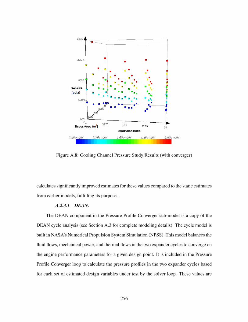
Figure A.8: Cooling Channel Pressure Study Results (with converger)

calculates significantly improved estimates for these values compared to the static estimates

from earlier models, fulfilling its purpose.

A.2.3.1 DEAN.

The DEAN component in the Pressure Profile Converger sub-model is a copy of the

DEAN cycle analysis (see Section A.3 for complete modeling details). The cycle model is

built in NASA’s Numerical Propulsion System Simulation (NPSS). This model balances the

fluid flows, mechanical power, and thermal flows in the two expander cycles to converge on

the engine performance parameters for a given design point. It is included in the Pressure

Profile Converger loop to calculate the pressure profiles in the two expander cycles based

for each set of estimated design variables under test by the solver loop. These values are

256

compared to the estimated pressure profiles using the root mean square error component to

determine the quality of the estimated values.

A.2.3.2 Pressure RMSE.

The purpose of the Pressure RMSE component is to compute the root mean square

error between the estimated pressure levels and the actual pressure levels in the two

expander cycles of the DEAN engine. The root mean square error is computed by taking

square root of the average of the squares of the difference between the expected and actual

values. Inspection of the source code demonstrated the component functioned correctly

and delivered the desired result.

Lines 2-3 compute the square root of the average value for the squares of the

differences for each cycle as computed by the mse function (Lines 6-16). The mse function

uses a for loop (Lines 10-12) to sum up the squares of the differences. Line 14 then divides

the sum by the number of stations in the given cycle to compute the average before returning

the average in Line 15.

Listing A.6: Pressure RMSE Source Code

1 function run() {2 LOX_RMSE.value = Math.sqrt(mse(Est_LOX_PressProfile, LOX_PressProfile));3 LH2_RMSE.value = Math.sqrt(mse(Est_LH2_PressProfile, LH2_PressProfile));4 }5

6 function mse(est, actual) {7 var n = est.length;8

9 var mse_val = 0;10 for (i = 0; i < n; i++) {11 mse_val = mse_val + (Math.pow(est.value(i) - actual.value(i),2));12 }13

14 mse_val = mse_val/n;15 return mse_val;16 }

A.3 Engine Cycle Analysis: Wall Thickness Converger

The engine cycle analysis portion of the DEAN model is defined by the Wall Thickness

Converger loop, shown in Figure A.9 and the analyses contained within it.

257

Figure A.9: Engine Cycle Analysis Components

There are five components contained in the Wall Thickness Converger loop. The first

is the DEAN cycle model. This component is the core of the DEAN analysis, using

NPSS to balance the two expander cycles. The second and third components are the

Angelino and Angelino Correction analyses. These components work together to create

an approximate geometry for the aerospike used in later sizing analyses. Finally, the fourth

and fifth components, in their own internal sizing loop, are the Cooling Jacket and Material

Properties components. These last two components work together to determine the wall

thickness for the cooling jackets in both the combustion chamber and the aerospike. The

outer converger loop iterates over these components until the guessed cooling jacket wall

thicknesses match the calculated wall thicknesses in the Cooling Jacket component.

A.3.1 DEAN.

As mentioned above, the DEAN cycle model, an NPSS model of the DEAN engine,

is the core of the system analysis for the DEAN engine. This component uses NPSS to

balance the fluid flows, mechanical power, and thermal flows in the two expander cycles

to converge on the engine performance parameters for a given design. The DEAN cycle

model, originally developed by David Martin as part of his thesis, remains essentially the

258

same in the DEAN system model [2]. Specifically, the modeling of the two expander

cycles is identical to Martin’s model except for the use of parametrization as documented in

Chapter 3 and an update to station numbering to make the model consistent with published

documentation. The primary changes in this version of the DEAN cycle model are updated

preprocessing calculations, to address the robustness of the model, the new parametrization

discussed in Section 4.3.1, and updated performance calculations, to eliminate the need for

TDK which greatly simplifies the system level model. The component was verified through

inspection of its source code.






connections are made using NPSS Application Programming Interfaces modeling fluid

flows, mechanical power, and thermal flows called “ports”. A built-in solver in NPSS

is then used to drive the model design variables to converge on a design point by balancing

the fluid flows, mechanical power, and thermal flows in the model [31].

The NPSS model of the DEAN engine includes elements to simulate the various

components of the engine. Many of the engine components are modeled using built-in

NPSS simulation elements. For example, the combustion chamber is modeled using a

RocketComb1 element and the aerospike nozzle is modeled using a RocketNozzle element.

The primary complexity in the NPSS DEAN model is in the elements used to model

the plumbing in the engine. This complexity is required to properly capture the fluid

and thermal flows which are critical to any expander cycle. These flows are the source

of the power used to drive the turbomachinery. The plumbing elements are modeled

using Valve04 elements to model the pressure drop in the plumbing and customized

259

CoolingVolume elements to model the heat loss in the lines. Wall2 elements are used

to connect the plumbing to the combustion chamber and the aerospike nozzle where the

plumbing functions as part of the cooling jackets. Full details of the NPSS modeling

elements used in the DEAN model can be found Section 3.2.2.

While the cooling jackets in the DEAN are continuous volumes, the NPSS model

represents them as a series of eight discrete stations. Figure A.10 shows the locations of

these stations in the model. The chamber consists of five equally spaced sections, with

stations (represented by dots) at the mid-point of each section plus a station at the engine’s

throat. The oxidizer loop (the outer wall of the chamber) and the fuel loop (the aerospike)

are represented by separate sets of stations. The external portion of the aerospike has two

additional stations in the first half of the nozzle only in the fuel loop.

Figure A.10: DEAN Geometry

The NPSS DEAN model source file is structured into five sections both to improve

readability and to simplify the process of bringing the model into the ModelCenter

environment. Only the first section (design variables) is intended to be edited during design

exploration, either by hand or by ModelCenter as part of automated trade studies. The

design variables section is a list of declarations for the top level design variables, including

the variables listed in Table A.2. Additional variables in this section include various initial

260

estimates required for NPSS independent variables. Table A.6 lists the critical independent

variables in this section of the model.

Table A.6: DEAN Independent Variables Listing


PRdes PumpO Initial estimate for the LOX pump pressure ratio

PRdes Pump1F Initial estimate for the first LH2 pump pressure ratio

PRdes Pump2F Initial estimate for the second LH2 pump pressure ratio

Ox Bypass Initial estimate for the percent of mass flow moving

through the oxidizer bypass

The second section, the constants section, lists the various physical constants used in

the model, including estimated values for enthalpy and density of the fluids in the expander

cycles and geometric values not specified by the design variables such as the cross sectional

area of the pipes. This section should only be edited as part of an update to the working

fluids in the model, for example changing the propellant from liquid hydrogen to liquid

methane. The third section, the derived values section, calculates the values required

by the NPSS elements from the design variables and constants in the previous sections.

The calculations in this section will be discussed below as part of the verification of the

DEAN cycle model. The fourth section, the DEAN section, contains the declarations of

the NPSS elements for the DEAN cycle model and the solver configuration and execution.

This section is the portion of the model which implements and balances the two expander

cycles. The fifth and final section, the output generation section, prints out a detailed report

of the results of the cycle balance from the fourth section. This report includes both overall

engine performance parameters such as thrust and specific impulse as well as detailed fluid

state values such as temperature and pressure at each station in both expander cycles. The

261

remainder of this section of the text will focus on the computational parts of the NPSS

DEAN model, namely the derived values and the DEAN sections.

The majority of the updates to the NPSS DEAN model occurred in the derived values

section. This section includes updated engine geometry calculations and calculations

to estimate the pressure levels in each expander cycle. The updated engine geometry

calculations include the inner and outer radii of the chamber and the throat, the chamber’s

average cross-sectional area, the nozzle length, and injection ratio which is the ratio of the

chamber cross-sectional area at the injector face to the throat area. Listing A.7 contains the

source code which calculates the overall engine geometry from the design variables.

Listing A.7: DEAN Geometry Calculations

1 // calculate outer throat and chamber radii2 real r_to = (Epsilon * A_throat / PI)**0.5; // outer throat radius3 real r_co = r_to + 1; // per design specs4

5 // calculate inner throat radius6 real r_ti = (r_to**2 - (A_throat / PI))**0.5; // inner throat radius7

8 // calculate chamber volume from L_star9 real V_c = Lstar * A_throat;

10

11 // calculate inner chamber radius from chamber volume12 // need some intermediate values: V2 and Z13 real V2 = PI * 0.2 * ChamberLength *14 (r_co**2 - (r_co**2 + r_co*r_to + r_to**2)/3);15

16 // use quadratic formula to get r_ci17 real A = 3;18 real B = r_ti;19 real C = (V_c - PI * r_co**2 * ChamberLength + V2 +20 0.2 * PI * ChamberLength * r_ti**2) / (0.2 * PI * ChamberLength);21 real r_ci = (-B + (B**2 - 4*A*C)**0.5) / (2*A);22

23 // chamber average area is volume / length24 real A_c = V_c / ChamberLength;25

26 // Chamber ratio is the ratio of A_c to A_t27 real chamberRatio = A_c / A_throat;28

29 // Injection ratio is the ratio of the30 // chamber area at the injection face to the A_t31 real A_ci = (r_co**2 - r_ci**2) * PI;32 real injectionRatio = A_ci / A_throat;33

34 // Vspike_int: SOLID INTERNAL AEROSPIKE VOLUME CALCULATION35 // 2 components: linear side and sloped side36 // Vspike_int = Vol1 + Vol237 // 1st Component: Linear Side

262

38 // Vol1 = pi*rˆ2*L (Volume of Cylinder)39 real Vol1 = 0.4 * PI * ChamberLength * r_ci**2;40

41 // 2nd Component: Sloped side starts between stations 2 and 342 // and goes to station 643 // Vol2 = Volume of Conical Frustum - sloped portion of chamber volume (inˆ3)44 // NOTE: Vol eqn is from http://mathworld.wolfram.com/ConicalFrustum.html45 real Vol2 = PI * 0.6 * ChamberLength * (r_ti**2 + r_ti * r_ci + r_ci**2)/3;46

47 // inˆ3, Solid Aerospike Volume Internal to Chamber48 real Vspike_int = Vol1 + Vol2;49

50 // find the nozzle length51 real r_t = (A_throat / PI)**0.5;52 real A_e = A_throat * Epsilon;53 real r_e = (A_e / PI)**0.5;54

55 // step 2: find total cone length and length of cone to throat56 real l_total = r_e / tan(alpha);57 real l_t = r_t / tan(alpha);58

59 // step 3: NozzleLength is the delta of l_total and l_t60 real nozzleLength = l_total - l_t;61 }

Line 2 uses the definition of the expansion ratio to find the outer throat radius. The

outer throat radius of the DEAN is the radius of the circle defining the exit area. Solving the

definition of the expansion ratio shown in Equation (A.1) for the exit area and substituting

the area of a circle for the exit area gives Equation (A.8). As noted above, the outer throat

radius, rto is the same as the exit radius, re. Making this substitution and solving for the

outer throat radius gives Equation (A.9), which is implemented by Line 1 of Listing A.7.

Based on Martin’s original definition of the chamber’s contour of the chamber, the chamber

outer radius is one inch greater than the throat outer radius. Line 3 implements this

calculation.

πr2e = εAt (A.8)

rto =√εAt/π (A.9)

The inner throat radius is the radius of the aerospike at the throat. This radius can be

found from the throat area and the outer throat radius. The throat area is the area of a disc,

263

which is shown in Equation (A.3). The outer radius in Equation (A.3) is the outer throat

radius, and the inner radius is the inner throat radius. Substituting these definitions, and

the throat area for the area of the disc, and then solving for the inner throat radius gives

Equation (A.10). Line 6 implements this calculation.

rti =

√rt

2o − At/π (A.10)

The chamber volume is calculated from the definition of characteristic length, shown

in Equation (A.11) [5]. Solving for the chamber volume gives Equation (A.12). Line 9

implements this calculation.

L∗ = Vc/At (A.11)

Vc = L∗At (A.12)

In the original parametrization of the DEAN cycle model, the chamber volume was

calculated from the inner and outer chamber and throat radii. Solving the calculations from

the original parametrization for the inner throat radius instead of the chamber volume yields

the calculations required to calculate the final radius in the DEAN engine. The chamber

volume is composed of three elements, shown in Figure A.11: a hollow cylinder running the

length of the chamber representing the volume displaced by the majority of the aerospike

nozzle referred to as Volume 1, the difference between a cylinder and a frustum with a

shared outer radius representing the volume removed from the chamber by the reduction

in chamber radius over the last 20% of the chamber (station 5 in Figure A.10) referred

to as Volume 2, and a hollow conical frustum representing the volume displaced by the

converging portion of the aerospike nozzle covering the last 60% of the chamber length

(stations 3-5 in Figure A.10) referred to as Volume 3.

264

Figure A.11: DEAN Chamber Volume Elements

Equation (A.13) gives the calculation in terms of this relationship. Equation (A.14)

uses the equation for the volume of a hollow cylinder to define the volume of Volume 1 in

terms of the chamber radii.

Vc = V1 − V2 − V3 (A.13)

V1 = πLc(rc2o − rc

2i ) (A.14)

Volume 2 is the volume removed by the reduction in chamber radius at the throat.

This volume is the difference between a cylinder with a radius equal to the chamber’s

outer radius and a frustum with r1 equal to the chamber’s outer radius and r2 equal to

the chamber’s inner radius. Equation (A.13) shows this relationship and Equation (A.16)

shows the calculation for the volume of a frustum. Expanding Equation (A.13) with the

definitions for Vc and V f gives Equation (A.17). Dividing out the common terms, πL,

gives Equation (A.18). Finally, substituting 20% of the chamber length for L, the outer

chamber radius for r, and the outer chamber and throat radii for r1 and r2 respectively gives

Equation (A.19) which calculates Volume 2.

265

V2 = Vc − V f (A.15)

V f =13πL(r2

1 + r1r2 + r22) (A.16)

V2 = πLr2 −πL3

(r21 + r1r2 + r2

2) (A.17)

V2 = πL(r2 − (r21 + r1r2 + r2

2)/3) (A.18)

V2 = 0.2Lcπ(rc2o − (rc

2o + rcorci + rc

2i )/3) (A.19)

Finally, Volume 3, the hollow conical frustum, represents the volume displaced by the

converging portion of the aerospike nozzle and can be calculated based on Equation (A.16).

For Volume 3, the inner radius of the hollow portion of the frustum is the same as the

second radius in the frustum volume equation. Subtracting the cylindrical volume for

this radius, πLr22, from Equation (A.16) gives the volume for a hollow frustum, shown

in Equation (A.20). Substituting 60% of the chamber length for L, and the inner throat and

chamber radii for r1 and r2 respectively gives Equation (A.21) which calculates Volume 3.

V f h =13πL(r2

1 + r1r2 − 2r22) (A.20)

V3 =0.6Lc

3π(rt

2i + rtirci − 2rc

2i ) (A.21)

Taken together, Equation (A.13), Equation (A.14), Equation (A.19), and Equation (A.21)

define how the chamber volume is calculated in the original parametrization of the DEAN

266

NPSS model. With the new parametrization, chamber volume is calculated from the char-

acteristic length as shown in Equation (A.12) and the inner chamber radius must be calcu-

lated from the relationships above. The inner chamber radius appears in the equations for

Volume 1 and Volume 3. The equation for Volume 3 is of the form of a quadratic equation

which can be solved using the quadratic formula with the proper algebraic transformations.

These transformations start with rearranging Equation (A.13) to solve for Volume 3 which

gives Equation (A.22).

V3 = −Vc + V1 − V2 (A.22)

Substituting the definitions of Volume 1 and Volume 3 into Equation (A.22) gives

Equation (A.23). Carrying out the division of 0.6Lc3 on the left hand side and distributing

the πLc on the right hand side gives Equation (A.24). Then, dividing both sides by 0.2Lcπ


0.6Lc

3π(rt

2i + rtirci − 2rc

2i ) = −Vc + πLc(rc

2o − rc

2i ) − V2 (A.23)

0.2Lcπ(rt2i + rtirci − 2rc

2i ) = −Vc + πLcrc

2o − πLcrc

2i − V2 (A.24)

rt2i + rtirci − 2rc

2i =−Vc + πLcrc

2o − πLcrc

2i − V2

0.2Lcπ(A.25)

The rci term on the right hand side needs to be brought over to the left hand side to

group all of the rci terms together. To do this, the rci is separated out on the right hand side

which gives Equation (A.26). Canceling out terms in πLcrc2i

0.2Lcπgives Equation (A.27). This

step gives the simplified value of −5rc2i on the right hand side which can be moved to the

left hand side giving Equation (A.28). Finally, moving the right hand side to the left hand

side gives Equation (A.29) which is in the standard form of a quadratic equation.

267


2i =−Vc + πLcrc

2o − V2

0.2Lcπ−πLcrc

2i

0.2Lcπ(A.26)


2i =−Vc + πLcrc

2o − V2

0.2Lcπ− 5rc

2i (A.27)

3rc2i + rtirci + rt

2i =−Vc + πLcrc

2o − V2

0.2Lcπ(A.28)

3rc2i + rtirci +

Vc − πLcrc2o + V2 + 0.2πLcrt

2i

0.2Lcπ= 0 (A.29)

With Equation (A.29) being a quadratic equation in standard form, the value of the

inner chamber radius can be solved using the quadratic formula, Equation (A.30) by letting

a = 3, b = rti, c equal the remaining terms and applying positive option for the ±. Lines

11-21 implement these calculations.

For ax2 + bx + c = 0

x =−b ±

√b2 − 4ac

2a

(A.30)

The next three calculations, Lines 24, 27, and 32 from Listing A.7, compute various

key ratios required for later calculations. The final blocks of code in Listing A.7 relate to

the geometry of the aerospike nozzle. Lines 34-48 calculate the volume of the portion of

the aerospike contained within the chamber using the volume of a cylinder and the volume

of a conical frustum similar to previous calculations. The remaining code estimates the

length of the external portion of the aerospike nozzle. According to Sutton and Biblarz,

the length of an aerospike nozzle can be estimated using the length of a conical nozzle

of the correct parameters. Sutton and Biblarz recommend setting the half angle equal of

the conical nozzle between 10 and 12 degrees and setting its expansion ratio equal to the

aerospike nozzle’s expansion ratio. Computing the length of a conical nozzle involves

268

calculating the difference in the heights of cones with the specified half angle. The first

cone has a base area equal to the throat area and the second cone has an area equal to the

exit area. Figure A.12 shows how these two cones relate to calculating the nozzle length

[24].

Figure A.12: Calculating Conical Nozzle Length

Lines 51-53 compute the radii for the bases of the cones with base areas of the throat

and the exit area. Lines 56-57 then compute the ltotal and lt shown in Figure A.12 using the

tangent relationship with the half angle alpha of 12 degrees, which was set in the constants

section of the model. Finally, Line 60 computes the actual nozzle length from the difference

of the other two lengths.

Listing A.8 shows the next block of code of the derived values section of the DEAN

cycle model. This block of code estimates the pressure levels in the two expander cycles

from the estimated specific impulse (TargetIsp) and notional pressure gains and losses

associated with the pumps, turbines, and plumbing.

Listing A.8: DEAN Estimated Pressure Level Calculations

269

1 // Calculate the estimated pressure profile2 real mdot = Thrust / TargetIsp;3 real mdotO = (O_F / (O_F + 1)) * mdot; //Oxidizer mass flow rate (lbm/s)4 real mdotH = mdot - mdotO; //fuel mass flow rate (lbm/s)5

6 // calculate P0_guess from mdot, c and a_t7 real P_c = mdot * c_star / (A_throat * g0);8

9 // calculate the LOX pressure profile10 int numLOX_stations = 11;11 real LOX_EstPresProfile[11];12 LOX_EstPresProfile[0] = P_TankO * .95; // start just below ox tank pressure13 LOX_EstPresProfile[1] = LOX_EstPresProfile[0] * PRdes_PumpO;14

15 // injector losses16 LOX_EstPresProfile[numLOX_stations-1] = P_c * (1 + injectorPressureLoss);17

18 // turbine losses19 LOX_EstPresProfile[numLOX_stations-3] =20 LOX_EstPresProfile[numLOX_stations-1] * 1.5;21

22 // bypass pressure23 LOX_EstPresProfile[numLOX_stations-2] =24 (LOX_EstPresProfile[numLOX_stations-1] +25 LOX_EstPresProfile[numLOX_stations-3])/2;26

27 // for loop to enter values into the cooling channel stations.28 // Assume linear pressure loss through the channels (6 stations)29 int i;30 for(i = 2; i < numLOX_stations - 3; i++) {31 // From station CVO1 to CVO1, subtract equal pressure drops32 // (linearly decrease) to get from exit of pump to entrance of turbine33 LOX_EstPresProfile[i] = LOX_EstPresProfile[i-1] -34 ((LOX_EstPresProfile[1] - LOX_EstPresProfile[numLOX_stations - 3]) / 7);35 }36

37 // stations (P_CVO#) are numbered forward to aft38 real P_OCV1 = LOX_EstPresProfile[0]; // Pressure for OCV1 (psia)39 real P_OCV2 = LOX_EstPresProfile[1]; // Pressure for OCV2 (psia)40 real P_CVO6 = LOX_EstPresProfile[2]; // Pressure for CVO6 (psia)41 real P_CVO5 = LOX_EstPresProfile[3]; // Pressure for CVO5 (psia)42 real P_CVO4 = LOX_EstPresProfile[4]; // Pressure for CVO4 (psia)43 real P_CVO3 = LOX_EstPresProfile[5]; // Pressure for CVO3 (psia)44 real P_CVO2 = LOX_EstPresProfile[6]; // Pressure for CVO2 (psia)45 real P_CVO1 = LOX_EstPresProfile[7]; // Pressure for CVO1 (psia)46 real P_OCV3 = LOX_EstPresProfile[8]; // Pressure for OCV3 (psia)47 real P_TBCV1 = LOX_EstPresProfile[9]; // Pressure for TBCV1 (psia)48 real P_OCV4 = LOX_EstPresProfile[10]; // Pressure for OCV4 (psia)49

50

51 // calculate the Fuel pressure profile52 int numH2_stations = 13;53 real LH2_EstPresProfile[13];54 LH2_EstPresProfile[0] = P_TankH * .95; // start just below fuel tank pressure55

56 //pump 1 pressure increase57 LH2_EstPresProfile[1] = LH2_EstPresProfile[0] * PRdes_Pump1F;58

59 //pump 2 pressure increase60 LH2_EstPresProfile[2] = LH2_EstPresProfile[1] * PRdes_Pump2F;61

270

62 // injector losses63 LH2_EstPresProfile[numH2_stations - 1] = P_c * (1 + injectorPressureLoss);64

65 // turbine losses (currently just a guess)66 LH2_EstPresProfile[numH2_stations - 2] =67 LH2_EstPresProfile[numH2_stations - 1] * 1.25;68

69 // for loop to enter values into the cooling channel stations.70 // Assume linear pressure loss through the channels (8 stations)71 for(i = 3; i < (numH2_stations - 2); i++) {72 //From station HCV1 to CVH1, subtract equal pressure drops (73 // linearly decrease) to get from exit of pump to entrance of turbine74 LH2_EstPresProfile[i] = LH2_EstPresProfile[i-1] -75 ((LH2_EstPresProfile[2] - LH2_EstPresProfile[numH2_stations-2]) / 9);76 }77

78 // stations (P_CVH#) are numbered forward to aft79 real P_HCV1 = LH2_EstPresProfile[0]; // Pressure for HCV1 (psia)80 real P_HCV2 = LH2_EstPresProfile[1]; // Pressure for HCV2 (psia)81 real P_HCV3 = LH2_EstPresProfile[2]; // Pressure for HCV3 (psia)82 real P_CVH8 = LH2_EstPresProfile[3]; // Pressure for CVH8 (psia)83 real P_CVH7 = LH2_EstPresProfile[4]; // Pressure for CVH7 (psia)84 real P_CVH6 = LH2_EstPresProfile[5]; // Pressure for CVH6 (psia)85 real P_CVH5 = LH2_EstPresProfile[6]; // Pressure for CVH5 (psia)86 real P_CVH4 = LH2_EstPresProfile[7]; // Pressure for CVH4 (psia)87 real P_CVH3 = LH2_EstPresProfile[8]; // Pressure for CVH3 (psia)88 real P_CVH2 = LH2_EstPresProfile[9]; // Pressure for CVH2 (psia)89 real P_CVH1 = LH2_EstPresProfile[10]; // Pressure for CVH1 (psia)90 real P_HCV4 = LH2_EstPresProfile[11]; // Pressure for HCV4 (psia)91 real P_HCV5 = LH2_EstPresProfile[12]; // Pressure for HCV5 (psia)

The pressure levels in both cycles are estimated using the same process, described

in detail for the LOX expander cycle and shown in Lines 9-48. The work flow for the

estimation process is to calculate the pressure gains from the pump(s) and the pressure

losses from the injector and turbine and then calculate the losses in the cooling channels

and other plumbing by linearly interpolating between the pressure level coming out of the

pump and the pressure level going into the turbine.

Lines 12-13 estimate the pressure gain in the LOX cycle by assuming a 5% loss from

the tank to the pump and a pressure gain from the pump based on the estimated pressure

ratio from the Pressure Profile Converger. The initial pressure ratio, PRdes PumpO,

is specified in the design variables section of the DEAN cycle model. Lines 16-20

estimate the pressure loss across the injector and turbine in the LOX cycle. The assumed

pressure loss across the injector is specified by multiplying the chamber pressure P c by

1 + in jectorPressureLoss. The in jectorPressureLoss variable is set to a value of 0.2 in

271

the constants section of the DEAN cycle model, which yields an injector pressure loss of

20% of the chamber pressure, the value recommended in Space Propulsion Analysis and

Design [5]. The pressure loss across the turbine is assumed to be 33% as specified by the

1.5 multiplier in Line 20.

This series of calculations requires an estimated chamber pressure, which is computed

in Lines 2-7. The estimated chamber pressure is based on three design variables: thrust,

throat area, and estimated specific impulse. The thrust and estimated specific impulse are

used to compute the weight flow in Line 2 based on Equation (A.6). Then in Line 7, the

computed weight flow and the throat area are combined with the characteristic exit velocity

(c∗) to compute the estimated chamber pressure according to Equation (A.7) [5]. The

value for the characteristic exit velocity is determined by the chemistry of the combustion

reactants, and is specified in the constants section of the DEAN cycle model.

The linear interpolation between the exit pressure from the LOX pump and the inlet

pressure at the LOX turbine is computed in the for-loop in Lines 30-35. Finally, Lines 38-

48 map the estimated pressure levels to variables used in the DEAN section of the model to

initialize the station pressures with the initial estimates. The same process is implemented

for the LH2 cycle in Lines 52-91. An additional set of calculations in the LOX cycle

on Lines 23-25 compute the pressure level in the bypass by averaging the pressure levels

before the turbine and the injector face.

While the majority of the updates to the DEAN cycle model occurred in the derived

values section, two key updates were made in the underlying model of the expander cycles.

The first of these changes is a simple renumbering of the stations to synchronize the model

with published documentation. The second change in the DEAN section of the NPSS

model is to the thrust calculation. In previous versions of the DEAN cycle model, the thrust

was calculated using the standard NPSS rocket nozzle element. This element calculates

rocket performance assuming a bell nozzle. Hall discusses the differences between the

272

calculations in the rocket nozzle element and aerospike nozzle theory in his thesis. In

particular, when the pressure profile across the aerospike is available, for example from an

analysis in TDK, the thrust for an aerospike nozzle can be calculated with Equation (A.31)

[4].

F = Fm + Fcowl + Fpressure + Fnondesign (A.31)

Comparing Hall’s results for total thrust, which include all four terms in Equation (A.31),

to the results using the standard NPSS rocket nozzle element showed the majority of the

difference between the two thrust values was in the Fnondesign term. This term accounts for

the thrust component from operating the engine above or below its design altitude. As can

be seen in Equation (A.32), Fnondesign is the result of the pressure difference between the

exit pressure and the ambient pressure acting on the exit area.

Fnondesign = (pe − pamb)Ae (A.32)

A modified rocket nozzle element was created to account for the Fnondesign term. This

new element simply adds the Fnondesign value to the total thrust calculated by the standard

bell nozzle analysis. Since the true exit area of an aerospike nozzle depends on the ambient

conditions and how those conditions affect the expansion of the exhaust flow, the updated

rocket nozzle component uses the design flow exit area, which is the minimum exit area for

an aerospike nozzle. Using the minimum exit area gives a conservative value for the total

thrust [4].

Listing A.9 shows the single modified line of the updated rocket nozzle element. The

first half of Line 1, (C f ∗ FlI .Pt ∗ Ath), is the bell nozzle thrust calculation. The second

half of the Line, ((FlI .Pt/PRexit − Ps) ∗ Ath ∗ AR), implements Equation (A.32) using

system parameters which are available in the nozzle element. The exit pressure (Pe) term is

computed from the exit pressure ratio (PRExit) and the chamber pressure (FlI .Pt) shown

273

in Equation (A.33). The exit area term (Ae) is computed from the expansion ratio shown

(AR) and the throat area (Ath) in Equation (A.1).

PRe =p0

pe(A.33)

Listing A.9: Aerospike Thrust Calculation

1 Fg = (Cf * Fl_I.Pt * Ath) + ((Fl_I.Pt/PRexit - Ps) * Ath * AR);

With no other changes to the cycle portions of the DEAN cycle model, the verification

of the model documented in Chapter 3 is still valid. Specifically, work by Arguello and

Strain demonstrated the converged pressure values calculated by the NPSS model agreed,

often to within a few percent, with independently developed Pumpal® and RITAL®

models of the two expander cycles. This agreement confirmed the underlying soundness

of the cycle balance in the NPSS model which drives the engine performance calculations.

This confirmation combined with the inspection of the geometry calculations, pressure

level estimates, and improved performance calculations show the DEAN cycle model

correctly predicts the DEAN’s performance for a given design, which validates this model.

A.3.2 Angelino and Angelino Correction.

The Angelino and Angelino Correction components act together to perform a single

analysis. The purpose of this unified analysis is to approximate the aerospike nozzle

geometry using a modified Angelino approximation in place of the TDK analysis in Hall’s

thesis. The combined analysis was verified through testing which compared the results

of the modified Angelino approximation to the results from Hall’s TDK analysis. Three

nozzle geometries (Martin’s and Hall’s similar thesis designs with similar maximum radius

and expansion ratio; and Hall’s design with the expansion ratio increased from 5.3 to 10)

were modeled in both Hall’s TDK analysis and the Angelino Approximation and Angelino

274

Correction components. The resulting geometry was graphically compared to verify the

correct function of the Angelino and Angelino Correction components.

Figure A.13, Figure A.14, and Figure A.15 indicate the Angelino approximation alone

significantly underestimates the radius of the aerospike nozzle for the majority of its length.

Given the nozzle geometry is used to calculate the mass of the nozzle current design point,

the linear approximation is in some ways a better fit than the Angelino approximation alone

because the linear approximation’s over estimate of volume will lead to conservative values

for mass.

Figure A.13: Comparison of Angelino Approximation to TDK (Martin Design Point)

The error between the Angelino approximation and the TDK analysis can be quantified

by calculating the volume for the surface of revolution for the two curves. The Structural

Jacket Size component implements this calculation. Table A.7 summarizes the results of

the error analysis. The average error in volume is nearly 34%, which supports the previous

conclusion that the Angelino component is not sufficiently modeling the nozzle geometry.

275

Figure A.14: Comparison of Angelino Approximation to TDK (Hall Design Point)

Figure A.15: Comparison of Angelino Approximation to TDK (Hall Design Point with

Expansion Ratio of 10)

The discrepancy between the Angelino and TDK results indicates the TDK design is

between the Angelino curve and the linear approximation. Applying a correction factor

to the Hall example, shown in Figure A.16, supports this assumption. Implementing this

276

Table A.7: Angelino Approximation Error Analysis

Test Case Volume, TDK (in3) Volume, Angelino (in3) Error (%)

Martin 199 138 31

Hall 223 143 36

Hall (ε = 10) 692 455 34

correction in the Angelino Correction component leads to similar results for the Hall design

with an aspect ratio of 10 as can be seen in the Figure A.17.

Figure A.16: Angelino Approximation Correction (Hall Design Point)

The improvements can be quantified using the same technique as above. Table A.8

summarizes the results. The improvements in the error are significant. The average is

down to 5.3%, and the worst error is under 10%. Given the current architecture decision to

bore out much of the aerospike’s volume to save mass, an average error in the full nozzle’s

volume of approximately 5% should be sufficient for the level of detail in the current model.

277

Figure A.17: Angelino Approximation Correction (Hall Design Point with expansion ratio

of 10)

Table A.8: Corrected Angelino Approximation Error Analysis

Test Case Volume, TDK (in3) Volume, Angelino (in3) Error (%)

Martin 199 194 2.5

Hall 223 202 9.4

Hall (ε = 10) 692 665 3.9

While a linear approximation of the nozzle geometry is sufficient to calculate the

heat transfer areas associated with the fuel expander cycle [4], calculations involving the

volume, and ultimately the mass of the nozzle benefit from a higher fidelity approximation.

As shown above, the Angelino and Angelino Correction components provide the required

fidelity. The Angelino component uses Angelino’s approximation method to create an

initial representation of aerospike nozzle. Note, Angelino’s approximation method assumes

the ratio of specific heats and molecular weight are constant across the nozzle, the reaction

278

is isentropic and adiabatic, and the flow through the throat is choked (Mach number equals

one) [4, 48].

As can be seen in Figure A.18, the geometry generated from the Angelino

approximation (Initial Angelino) includes points to the left of the y-axis. These points

represent geometry inside the chamber and need to be removed to coordinate the nozzle

geometry with the internal chamber geometry of the DEAN. Removing these points is

the first function of the Angelino Correction component. The second function of the

Angelino Correction component is to implement the correction factor documented above.

The resulting geometry from both corrections is included in Figure A.18.

Figure A.18: Coordinating Angelino Approximation with Chamber Geometry

The generated geometry can be used in the remaining components of the DEAN

model in place of the TDK generated geometry, satisfying the required output of the

components. Further, these components adjust the geometry to match the current design’s

chamber geometry and combustion performance as was demonstrated in the verification

tests involving design points of different chamber dimensions and engine performance.

279

Providing the required nozzle geometry over a range of designs meets the purpose of these

components.

A.3.3 Cooling Jacket.

The purpose of the Cooling Jacket component is to size the cooling channel walls and

to calculate the wall temperatures as a percentage of their melting points. The component

was verified through inspection.

The Cooling Jacket component is a ModelCenter script component which implements

a solver loop in order to iteratively run the Material Properties component. For each

station in both the chamber and the aerospike, the Cooling Jacket component calculates

the maximum value between the bending and shear stress at that station and the wall

temperature. The component then compares the maximum stress to the limiting values

from the Material Properties component for the calculated wall temperature, selected

material, and the selected failure mode (ultimate or yield strength). If the stress is greater

than one or more limiting values, the wall thickness is incremented and the analysis is

repeated until the wall has sufficient thickness to prevent failure. It is important to note

the wall temperature increases with greater wall thickness leading to lower strengths in the

materials. This process can lead to designs with wall thicknesses on the order of inches

instead of hundredths of an inch resulting in very low thrust-to-weight ratios.

Initial inspection of the source code for the Cooling Jacket showed it had a number of

errors and repeated code blocks making inspection and error correction overly complicated.

Before continuing with the verification process, the component’s implementation was

refactored to minimize duplicated code and improve readability. During the refactoring

effort, the various errors were corrected and repeated code blocks were placed in user

defined functions.

With the errors in the Cooling Jacket Analysis corrected the inspection could continue

with a focus on the implementation of the governing equations. The governing equations

280

for the Cooling Jacket analysis code include the calculation of the bending moment, the

calculation of the bending stress, the calculation of the shear stress, and the calculations of

the wall temperatures on the hot and cold sides. During the inspection, the source code for

each of these calculations was compared to the governing equations.

The stresses in the cooling jackets are calculated from the stresses in the individual

cooling channels. A simplified view of the cooling channels’ design, neglecting the

curvature of the engine, is shown in Figure A.19. Along the top of the figure is the

structural jacket. followed by the optional cooling jacket cover used when the structural

jacket material is not compatible with the propellant. The bottom of the figure is a cross-

section of half of a cooling channel. Inside the channel is the high pressure propellant

and outside the channel, at the bottom of the figure, is the combustion chamber. From

this view, it is clear each cooling channel can be modeled as a beam with fixed supports

under a uniform load from the pressure difference between the propellant and the chamber

pressures.

Figure A.19: Cooling Channel Design - Cross-Section View [4]

281

To incorporate the engine’s curvature, the cooling channels are modeled as curved

beams instead of simple beams under the uniform load and using the fixed supports noted

above. The bending moment for such beams is shown in Equation (A.34) [70].

Mx =w12

(6lx − 6x2 − l2) (A.34)

Listing A.10 shows the function which calculates the bending moment. It is a direct

implementation of Equation (A.34).

Listing A.10: Cooling Jacket Bending Moment Function

1 function Beam_Moment(load, width, position) {2 return (load/12)*(6*width*position - 6*Math.pow(position,2) -3 Math.pow(width,2));4 }

The equations for the bending stress in a curved beam on the inner and outer surface

are given by Equation (A.35) and Equation (A.36) respectively [70]. The source code in

Listing A.11 implements these equations. [Note, the division by 1000 in the source code is

to convert the results from psi to ksi.] A simple inspection shows the source code correctly

implements the governing equations.

σi =Mci

Aeri(A.35)

σo =Mco

Aero(A.36)

Listing A.11: Cooling Jacket Bending Stress Calculations

1 var sigma_bending_in = (M * ci) / (A * e * ri) / 1000; //ksi, Inner stress2 var sigma_bending_out = (M * co) / (A * e * ro) / 1000; //ksi, Outer stress

282

The maximum shear stress for a rectangular cross-section is shown in Equation (A.37)

where the value for S in a beam with fixed supports is given by Equation (A.38). The source

code in Listing A.12 implements these equations (and incorporates the factor of safety in

the final answer). Line 1 calculates the actual maximum shear stress from Equation (A.38)

where load (w) equals pressure difference (load), the length (l) equals the channel width

(width), the x-coordinate is set to the location of maximum shear stress, 0, and the area

(A) is computed from the height (h) and length (b) of the channel. Line 2 then applies the

factor of safety and converts the result from psi to ksi.

τmax =32

SA

(A.37)

S =w2

(l − 2x) (A.38)

Listing A.12: Cooling Jacket Shear Stress Calculations

1 var tau = (3/2) * (load * width / 2) / (h * b); //psi, Shear Stress2 tau_max = tau * fs.value / 1000; // ksi, Max shear stress w/fs

Calculating the wall temperatures involves solving the thermodynamic equilibrium

condition shown in Equation (A.39). Using the definition for enthalpy (h) in Equation (A.40),

one can get an equation for Q, Equation (A.41). Equation (A.42) and Equation (A.43) ex-

pand Equation (A.41) to define Qin and Qout, which when substituted into Equation (A.39)


Qin = Qout (A.39)

h =Q

A∆T(A.40)

283

Q = hA∆T (A.41)

Qin = HTH AH(THW − T0) (A.42)

Qout = HTC AC(Tcool − TCW) (A.43)

HTH AH(THW − T0) = HTC AC(Tcool − TCW) (A.44)

Equation (A.44) can be rearranged to form Equation (A.45). Let the value C equal

the left hand side of Equation (A.45), as shown in Equation (A.46) The hot side wall

temperature (THW) can be introduced by adding and subtracting it from the numerator,

as shown in Equation (A.47). Recall the heat flow (Hx) is defined as the difference in

temperatures between the two sides of the wall, Equation (A.48). Substituting Hx into

Equation (A.47) yields Equation (A.49).

Tcool − TCW

THW − T0=

HTH AH

HTC AC(A.45)

C =Tcool − TCW

THW − T0(A.46)

C =Tcool + THW − TCW − THW

THW − T0(A.47)

Hx = THW − TCW (A.48)

C =Tcool + Hx − THW

THW − T0(A.49)

284

Multiplying both sides by the (THW − T0) gives Equation (A.50). Rearranging

Equation (A.50) yields Equation (A.51) which has the hot wall temperature values all on

one side of the equation. Gathering the hot wall terms on the left hand side of the equation

gives Equation (A.52), which can then be simplified to Equation (A.53) to give a solution

for the hot side wall temperature in terms of the heat flow, the coolant fluid temperature,

the chamber temperature, and the value C defined above in Equation (A.46).

CTHW −CT0 = Tcool + Hx − THW (A.50)

CTHW + THW = Tcool + Hx + CT0 (A.51)

THW(1 + C) = Tcool + Hx + CT0 (A.52)

THW =Tcool + Hx + CT0

(1 + C)(A.53)

The values necessary to calculate C are available from the DEAN cycle model, as are

the coolant fluid temperature and the chamber temperature. The heat flow is then calculatd

in order to determine the hot side wall temperature. Begin with Equation (A.54), as defined

in Hall’s thesis Equation (14). Substituting the −Hx for (TCW −THW) from the definition of

Hx in Equation (A.48) gives Equation (A.55). Solving for Hx gives Equation (A.56).

q =−k∆l

(TCW − THW) (A.54)

q =k∆l

Hx (A.55)

Hx =q∆lk

(A.56)

285

The DEAN cycle model reports the total Q, instead of the normalized q. Equa-

tion (A.57) defines the relationship between these two terms. Using this definition to re-

place q with Q gives a form of the calculation of heat flow which can be calculated from

values available from the DEAN cycle model, shown in Equation (A.58).

q =QA

(A.57)

Hx =Q∆lkA

(A.58)

Finally, the cold side wall temperature can be calculated simply by rearranging the

definition of heat flow, Equation (A.48), to give Equation (A.59).

TCW = THW − Hx (A.59)

Equations (A.47), (A.53), (A.58), and (A.59) form the complete set of governing

equations necessary to calculate the wall temperatures. The source code in Listing A.13

implements these equations for each station in the Cooling Jacket.

Listing A.13: Cooling Jacket Wall Temperature Calculations

1 C = (HTCoefHot.value(i) * A_HxHot.value(i)) /2 (HTCoefCool.value(i) * A_HxCool.value(i));3 Hx_flow = (Qwall.value(i) * channel_thickness) / (k *A_HxHot.value(i));4 wall_temp_hot.value(i) = (Hx_flow + fluid_temp.value(i) + C*T0.value)/(1+C);5 wall_temp_cold.value(i) = wall_temp_hot.value(i) - Hx_flow;

Lines 1 and 2 implement Equation (A.47), Line 3 implements Equation (A.58), Line

4 implements Equation (A.53), and Line 5 implements Equation (A.59). A review of each

of these lines shows the source code correctly implements the governing equations.

Inspection of the Cooling Jacket component shows it correctly calculates the internal

stresses and temperatures of the cooling channel walls, and uses these values with the

values from the Material Properties component to determine the required thickness for the

286

cooling channel walls. These calculations fulfill the purpose of the component which is to

size the cooling channel walls and report their temperatures.

A.3.3.1 Material Properties.

The purpose of the Material Properties component is to report key material properties

(density, thermal conductivity, melting point, and strengths) for the materials under

consideration for the various elements in the DEAN design based on the element

temperatures. The Material Properties component was verified through inspection and

testing.

The Material Properties component is essentially a database of material properties

by temperature with sets of variables for each of the major elements of the DEAN

design (chamber cooling and structural jackets, aerospike cooling and structural jackets,

aerospike tip, and the plumbing for both the LOX and the LH2). The data reported by

this component (and the sources of this data) are tabulated in Hall’s masters thesis in

Appendix B. Tests for this component to verify its function include manual inspections of

the enumerated materials for each element to ensure the component complies with material

compatibility with the propellants, comparing the component’s reported material properties

to the tabulated data in Hall’s thesis, and inspection of the material property tables to

ensure each material supports a sufficient range of temperatures for thermal conductivity

and strengths.

Table A.9 shows the material selections available for each element of the DEAN

design. Each column lists an element of the DEAN design, and each row lists a material.

An ‘X’ in a particular cell indicates the material is included in the component as a material

option for the corresponding element. An ‘x’ in a particular cell indicates the material is

compatible with the corresponding element of the DEAN design as documented by Hall.

With this code, the component passes this manual inspection if there are only blank cells

or cells which contain ‘Xx’. The component does not pass if there are any cells with a

287

single ‘X’ or ‘x’. Two cells have single x’s in them, the cells which represent using silicon

carbide for the LOX and LH2 plumbing indicating the material is compatible with the

propellants, but is not an available option in the component. As noted above, this should

indicate an error in the component, however, in this case, the option was left out of the

component due to the difficulty in using silicon carbide to manufacture plumbing. With no

other discrepancies in the table, the component passes this verification test.

Table A.9: Component Material Compatibility Analysis

Material Chamber

CJ

Chamber

SJ

Spike

CJ

Spike

SJ

Spike

Tip

LOX

Plumb

LH2

Plumb

Pure Cu Xx Xx Xx Xx Xx Xx Xx

Silicon Carbide Xx Xx Xx Xx Xx xa xb

INCOLOY 909 Xx Xx Xx Xx Xx Xx Xx

Alloy 188 Xx Xx Xx Xx Xx Xx Xx

Beryllium Cu Xx Xx Xx Xx Xx Xx Xx

Ox-Free Cu Xx Xx Xx Xx Xx Xx Xx

Cobalt Xx Xx Xx Xx Xx Xx Xx

INCONEL 718 Xx Xx Xx

INCONEL 625 Xx Xx Xx

AL 7075 T6 Xx Xx

AL 2024 T6 Xx Xx

Titanium Xx

Niobium Xx

awhile compatible with LOX, silicon carbide is not suitable as a plumbing materialbwhile compatible with LH2, silicon carbide is not suitable as a plumbing material

288

A standalone model was developed to test the material properties reported by the

component. The model includes the Material Properties component and a top-level input

variable to set the temperature being tested. This top-level variable is linked to all of the

temperature input variables (including each element of the fluid temperature arrays) in

order to drive all of the element properties to the same values. Since several of the material

properties reported by the Materials Properties component are nonlinear, the component

returns step functions for each property. For temperatures below the minimum tabulated

value and above the maximum tabulated value, the component returns the property value

corresponding to the minimum and maximum temperatures respectively. Finally, Hall

reported constant density for each material as the density is only used in the mass

calculation, assumed to occur when the engine is not operating and is at room temperature.

The test procedure for the component began by setting the material selections for

each element to the same material (for example Beryllium Copper). A parametric study

was then run over the range of temperatures included in Hall’s data for the material under

consideration (for example 500R to 900R in three steps for Beryllium Copper). The results

of this trade study were then compared to Hall’s data to ensure consistency. Table A.10

is an example results set for the component (using Beryllium Copper) and Table A.11 is

the expected results from Hall’s thesis. Comparing these two tables shows the Beryllium

Copper results pass this verification test. Similarly, the component passes this verification

tests for the entire set of included materials.

289

Table A.10: Parametric Study Results for Beryllium Copper

Output Variable 500 (R) 700 (R) 900 (R)

Chamber Cool Rho (lbm/in3) 0.298 0.298 0.298

SJChamber Rho (lbm/in3) 0.298 0.298 0.298

Spike Cool Rho (lbm/in3) 0.298 0.298 0.298

SJSpike Rho (lbm/in3) 0.298 0.298 0.298

Spike Tip Rho (lbm/in3) 0.298 0.298 0.298

O2Pipe Rho (lbm/in3) 0.298 0.298 0.298

LH2Pipe Rho (lbm/in3) 0.298 0.298 0.298

Chamber Cool Melt (R) 2050.67 2050.67 2050.67

Spike Cool Melt (R) 2050.67 2050.67 2050.67

Chamber Cool k (BTU/in-R-s) 0.001578 0.001939 0.001939

Spike Cool k (BTU/in-R-s) 0.001578 0.001939 0.001939

Chamber Cool Ft (103 psi) 180 180 180

SJChamber Ft (103 psi) 180 180 180

Spike Cool Ft (103 psi) 180 180 180

SJSpike Ft (103 psi) 180 180 180

O2Pipe Ft (103 psi) 180 180 180

LH2Pipe Ft (103 psi) 180 180 180

Chamber Cool Fy (103 psi) 155 155 155

SJChamber Fy (103 psi) 155 155 155

Spike Cool Fy (103 psi) 155 155 155

SJSpike Fy (103 psi) 155 155 155

O2Pipe Fy (103 psi) 155 155 155

LH2Pipe Fy (103 psi) 155 155 155

290

Table A.11: Expected Results for Beryllium Copper [4]

Property Any T T < 527.67 (R) 527.67 (R) ≤ T

Density (lbm/in3) 0.298

Melting Point (R) 2050.67

Thermal Conductivity k (BTU/in-R-s) 0.00158 0.00194

Ultimate Tensile Strength (103 psi) 180

Yield Strength (103 psi) 155

The final verification process reviewed the material tables to ensure they provide

sufficient range of values by temperature to cover range of temperatures for thermal

conductivity and strengths. A limited range of temperatures for thermal conductivity

disqualified the material as an option for cooling jackets as the thermal conductivity is a

key factor in the performance of the cooling jacket. Similarly, a limited range of strengths

disqualified the material as an option for either the cooling or structural jackets and the

plumbing as the performance of these components is driven by their strengths. The property

tables for each material were inspected using the number of entries and the thermal range

covered by those entries used to judge the material’s fitness for inclusion in the model.

Two materials were disqualified for use in cooling jackets and one material was

disqualified for use in structural jackets and plumbing. Oxygen-free copper only has one

value for it thermal conductivity, which is at room temperature, disqualifying it for use with

cooling jackets. Beryllium copper only has one value for its strength, which is also at room

temperature, disqualifying it for use with cooling jackets, structural jackets, and plumbing.

Given the high temperatures seen in liquid rocket engines and the effects of high

temperatures on the material properties used in the DEAN model, these effects clearly

needed to be included in the DEAN model. The verification tests demonstrated the Material

Properties component, when the two disqualified materials were ignored, provides the

291

required temperature dependent material properties for each material option available in

a DEAN design, meeting the purpose of this component.

A.4 Post Processing Step 1: Performance

The Performance sequence, shown in Figure A.20, contains the Thrust-to-Weight

Calculation, with its supporting analyses the Channels and Structural Jacket Size analyses,

and the Pressure Profiles component which renders the pressure levels for both the LOX

and the LH2 expander cycles.

Figure A.20: Performance Sequence

A.4.1 Channels.

The purpose of the Channels component is to take the vector channel dimension data

returned by the DEAN cycle model and convert this data to scalar values to be used for

subsequent analyses. The component was verified by inspecting its source code.

The primary conversion used in this component is to average the channel wall

thicknesses to provide the Structural Jacket Size component with an inner wall thickness

for the chamber and the aerospike. To ensure the average wall thicknesses represent the

actual wall thickness of the chamber and the aerospike, the component also calculates

differences between the minimum and maximum wall thickness for both the chamber and

the aerospike. These differences are then used as constraints to ensure the variation in the

wall thicknesses is acceptable. Finally, the component also calculates the minimum channel

spacing for the LOX and LH2 cooling channels for use as a design constraint.

292

The calculations involved in the Channels analysis are simple averaging and

calculation of the minimum and maximum values in arrays. A single JavaScript function,

shown in Listing A.14 iterates over input arrays and records the minimum and maximum

values while calculating the average. This function is then called for the LOX and LH2

channel thickness arrays and the LOX and LH2 channel spacing arrays.

Listing A.14: Channels Component Average Function

1 function average(values) {2 var avg = 0;3 var numVals = values.length;4 var min = values.value(0);5 var max = values.value(0);6

7 for (var i = 0; i < numVals; i++) {8 avg += values.value(i);9

10 if (values.value(i) < min)11 min = values.value(i);12

13 if (values.value(i) > max)14 max = values.value(i);15 }16

17 avg = avg / numVals;18

19 return [avg, min, max];20 }

Inspection of the Channels component showed it properly converts the DEAN

analysis’ vector results to suitable scalars, with appropriate constraints, for use by the

Structural Jacket sizing analysis, meeting the purpose of this component.

A.4.2 Structural Jacket Size.

The purpose of the Structural Jacket Size component is to determine the wall thick-

nesses for the chamber and aerospike structural jackets and the engine’s plumbing. Ad-

ditionally, this component calculates geometric parameters for various engine components

including the plumbing cross-sectional area, the volume and weight of the structural jack-

ets, the volume and weight of the cooling channel covers if present, and the volume and

mass of the uncooled aerospike tip. The component was verified through inspection.

293

The DEAN engine has two structural jackets, one for the chamber and one for the

aerospike. The cross-section shown in Figure A.21 shows DEAN structural jackets in

relation to the cooling jackets and the ambient environment. The chamber, the black disc in

the figure, is a high pressure region and the ambient environment is a low pressure region.

Observe how the chamber structural jacket is containing the pressure from the chamber

internally and is therefore experiencing stress in tension. Conversely, the aerospike

structural jacket is containing the pressure from the chamber externally and is therefore

experiencing stress in compression.

Figure A.21: Cross-Section of the DEAN Engine

The Structural Jacket Size component computes the structural jacket sizes by solving

for the minimum wall thicknesses which yield a maximum stress in the structural jackets

within the stress limit for the selected material, including the model’s factor of safety. As

part of this calculation, the wall thicknesses are increased or decreased until the stress limit

is just met. The Structural Jacket Size component performs this analysis for the highest

294

pressure differential instead of one for each station. The system level model assumes a

nearly uniform temperature in the structural jacket, and in turn constant material properties

along the length of the engine. The highest pressure differential is calculated from the

difference between the maximum pressure in the related cooling channel and the ambient

pressure.

As with the Cooling Jacket component, initial inspection of the source code for the

Structural Jacket Size component showed it had a number of errors and repeated code

blocks making inspection and error correction overly complicated. Before continuing

with the verification process, the component’s implementation was refactored to minimize

duplicated code and improve readability. During the refactoring effort, the various errors

were corrected and repeated code blocks were placed in user defined functions.

With the errors in the Structural Jacket Size component corrected, the inspection could

continue with a focus on the implementation of the governing equations. The governing

equations for the Structural Jacket Size analysis include the radial and tangential stress in

a thick walled pressure vessel and the volumes for the various components of the DEAN.

During the inspection, the source code for each of these calculations was compared to its

governing equation and assumptions.

Equation (A.60) shows the calculation for the tangential stress in a thick walled

cylinder [70]. Listing A.15 shows the function which calculates the tangential stress. It

is a direct implementation of Equation (A.60)

σt =pir2

i − por2o − r2

i r2o(po − pi)/r2

r2o − r2

i

(A.60)

295

Listing A.15: Tangential Stress in a Thick Walled Cylinder Function

1 function sigma_tan(ri, ro, r, Pi, Po) {2 return (Pi*Math.pow(ri,2) - Po * Math.pow(ro,2) -3 Math.pow(ri,2) * Math.pow(ro,2) * (Po-Pi) / Math.pow(r,2)) /4 (Math.pow(ro,2)-Math.pow(ri,2));5 }

The calculation for the radial stress in a thick walled cylinder is very similar to the

calculation for the tangential stress, as can be seen in Equation (A.61). In both of these

equations, positive values indicate the cylinder is in tension, as would be expected for the

chamber’s structural jacket, and negative values indicate the cylinder is in compression, as

would be expected for the aerospike’s structural jacket [70].

σr =pir2

i − por2o + r2

i r2o(po − pi)/r2

r2o − r2

i

(A.61)

Listing A.16 shows the function calculating the radial stress. It is a direct

implementation of Equation (A.61)

Listing A.16: Radial Stress in a Thick Walled Cylinder Function

1 function sigma_tan(ri, ro, r, Pi, Po) {2 return (Pi*Math.pow(ri,2) - Po * Math.pow(ro,2) +3 Math.pow(ri,2) * Math.pow(ro,2) * (Po-Pi) / Math.pow(r,2)) /4 (Math.pow(ro,2)-Math.pow(ri,2));5 }

With these two calculations implemented, the remaining code for calculating the

structural jacket thickness is a straight forward loop over increasing or decreasing thickness

values until the stress limit is just satisfied. Listing A.17 shows the function which

implements this sizing loop.

296

Listing A.17: Calculate Wall Thickness Function

1 // tension can take on two values: 1 == in tension, -1 == in compression2 function calculateWallThickness(ri, ro, t, Pi, Po, stressLimit, tension) {3 // initialize variables4 var r = 0.0;5 var stepSize = 0.001;6 if (tension == 1) {7 r = ri;8 }9 else {

10 r = ro;11 }12

13 var maxStress = 0.0;14 if (tension == 1) {15 maxStress = fs.value * Math.max(sigma_tan(ri, ro, r, Pi, Po),16 sigma_rad(ri, ro, r, Pi, Po)) / 1000;17 }18 else {19 maxStress = fs.value * Math.min(sigma_tan(ri, ro, r, Pi, Po),20 sigma_rad(ri, ro, r, Pi, Po)) / 1000;21 }22

23 // multiply by tension to adjust for tension vs compression24 if (maxStress < stressLimit * tension) {25 while (maxStress < stressLimit * tension) {26 if (tension == 1) {27 t = t - stepSize;28 ro = ri + t;29 maxStress = fs.value * Math.max(sigma_tan(ri, ro, r, Pi, Po),30 sigma_rad(ri, ro, r, Pi, Po)) / 1000;31 }32 else {33 t = t + stepSize;34 ri = ro - t;35 maxStress = fs.value * Math.min(sigma_tan(ri, ro, r, Pi, Po),36 sigma_rad(ri, ro, r, Pi, Po)) / 1000;37 }38 }39 }40 else {41 while (maxStress > stressLimit * tension) {42 if (tension == 1) {43 t = t + stepSize;44 ro = ri + t;45 maxStress = fs.value * Math.max(sigma_tan(ri, ro, r, Pi, Po),46 sigma_rad(ri, ro, r, Pi, Po)) / 1000;47 }48 else {49 t = t - stepSize;50 ri = ro - t;51 maxStress = fs.value * Math.min(sigma_tan(ri, ro, r, Pi, Po),52 sigma_rad(ri, ro, r, Pi, Po)) / 1000;53 }54 }55 }56

297

57 return t;58 }

One important detail about this function is the purpose and use of the function

argument tension. The function argument tension is a flag indicating whether the sizing

loop is being run for a cylinder in tension (tension = 1) or compression (tension = −1).

Naturally, the function is called with a value of 1 for the chamber’s structural jacket, and

a value of −1 for the aerospike’s structural jacket. The argument is used in one of two

ways throughout the function. First, it is used as a test condition in if statements such as in

Lines 6, 14, 26, and 42, where it controls whether the calculation should be performed for

a tension or compression case. Second, it is used as a sign adjustment for the maximum

stress in the cylinder such as in Lines 24 and 41. For cases where the cylinder is in tension,

the stress values will be positive, as noted above, and the tension argument has a value of

1. When the positive stress value is multiplied by the tension value of 1, the stress value

remains positive. For cases where the cylinder is in compression, the stress values will be

negative, as noted above, and the tension argument has a value of −1. When the negative

stress value is multiplied by the tension value of −1, the stress value becomes positive.

The remainder of this function performs the iterations which increase or decrease

the wall thickness from the starting value provided by the function argument t until the

stress limit is just met using a pair of while loops. The first while loop, shown in lines

25-38, implements the decreasing case for cylinders in tension, and the increasing case

for cylinders in compression. This reversal of implementations is required because in

compression cases, the smaller stress value is a more negative number, representing a larger

magnitude of stress meaning the stress limit has been exceeded. The second while loop,

shown in Lines 41-54, similarly implements the increasing case for cylinders in tension,

and the decreasing case for cylinders in compression.

298

The plumbing thicknesses, one for LOX and one for LH2, are calculated by again

calling the calculateWallThickness function, this time using the difference between the

maximum fluid pressure in the cooling lines and ambient pressure for the pressure

difference. The cross-sectional area for the plumbing is calculated by computing the area

of an annulus, shown previously in Equation (A.3), with inner radius equal to the specified

plumbing radius and the outer radius equal to the plumbing radius plus the plumbing

thickness.

The remainder of the Structural Jacket Size component calculates the volumes for the

structural jackets, the cooling jacket covers, and the uncooled aerospike tip. The weight

of these components is calculated by simply multiplying the density of the component

materials by the calculated volumes. As can be seen in Figure A.21, the DEAN engine

is made up of a series of concentric elements, starting from the outside with the chamber

structural jacket and working down to the aerospike’s structural jacket. To calculate the

volume of a particular element, the Structural Jacket Size component calculates the volume

of the solids representing the outer and inner radii of the element, and then computes

the difference between these two volumes. Each element is composed of one or more

geometric primitives including cylinders, frustums, and surfaces of revolution. Specifically,

the chamber structural jacket, and the chamber cooling jacket cover, are composed of

a cylinder and a frustum. The aerospike structural jacket is composed of one or two

cylinders depending on the inner most radius of the aerospike, two frustums, and a volume

of revolution for a portion of the curve defined by the Corrected Angelino component.

Finally, the solid aerospike tip is composed entirely of a volume of revolution for another

portion of the curve defined by the Corrected Angelino component.

The code which calculates of the volume of a cylinder is straight forward, as it

implements V = πr2h. However, the volume for a frustum and a volume of revolution

are more complicated and should be handled more carefully. Recall a frustum is essentially

299

a cone with the point removed. Equation (A.16) shows the calculation for the volume of a

frustum. Listing A.18 shows the function which computes this value. As can be seen, it is

a direct implementation of Equation (A.16).

Listing A.18: Frustum Volume Function

1 function frustumVolume(length, r1, r2) {2 // from http://mathworld.wolfram.com/ConicalFrustum.html3 return 1/3 * Math.PI * length *4 (Math.pow(r1,2) + (r1*r2) + Math.pow(r2,2));5 }

Calculating a volume of revolution requires solving the integral shown in Equation (A.62).

The Structural Jacket Size component uses the trapezoid method to numerically compute

this integral. Equation (A.63) shows this numerical solution. To simplify the implemen-

tation, the cross-sectional area, A(x) is precomputed using the definition found in Equa-

tion (A.64) [71].

V =

∫ b

aA(x)dx (A.62)

∫ b

aA(x)dx =

12

N∑2

(xi − xi−1) ∗ (A(xi−1) + A(xi)) (A.63)

A(x) = π[ f (x)]2 (A.64)

Listing A.19 shows the implementation of the volume of revolution equations for the

uncooled portion of the aerospike. Similar code is used to compute the volume of revolution

required for the cooled portion of the aerospike. The calculations start with the for loop in

lines 2-8 which compute the cross-sectional areas for the values of x which will be used in

the volume of revolution. This step corresponds to Equation (A.64). Lines 10 and 11 then

initialize the summation value and the Ai−1 value, represented by the variable prev A. The

for loop in Lines 12-17 then implements the summation in Equation (A.63), except for the

300

division by two which can be factored out of the summation. Finally, Line 19 applies the

factored out division by 2 to reach the final numerical solution for the volume of revolution.

Listing A.19: Volume of Revolution Volume Calculation

1 cross_area_nozz.length = spike_length_nozz.length;2 for (i = 0; i < spike_radius.length; i++) {3 if (spike_length_nozz.value(i) != 0) {4 cross_area_nozz.value(i) = Math.PI * Math.pow(spike_radius.value(i), 2);5 } else {6 cross_area_nozz.value(i) = 0;7 }8 }9

10 var sum = 0;11 var prev_A = cross_area_nozz.value(i_val);12 for (i = i_val + 1; i< cross_area_nozz.length; i++) {13 this_A = cross_area_nozz.value(i);14 sum += (spike_length_nozz.value(i) - spike_length_nozz.value(i-1)) *15 (this_A + prev_A);16 prev_A = this_A;17 }18

19 Vspike_tip.value = sum * 0.5;

Inspection of the Structural Jacket Size component shows it correctly calculates the

internal stresses of the structural jacket walls and the plumbing, and uses these values

to determine the required thickness for the structural jackets and plumbing. Further,

inspection shows this component properly calculates the volumes for these elements. These

calculations fulfill the purpose of the component: to size the structural jackets for both the

chamber and the aerospike.

A.4.3 Thrust-to-Weight Calculation.

The purpose of the Thrust-to-Weight Calculation component is to calculate the total

engine weight by estimating and summing up component weights, and then calculating the

thrust-to-weight ratio from total engine weight and engine thrust. This analysis estimates

weights for the following engine components: the chamber (made up of the chamber

cooling and structural jackets), the aerospike (made up of the aerospike cooling and

structural jackets and the uncooled tip), the LOX and LH2 turbopumps, the plumbing, and

the miscellaneous hardware. The Thrust-to-Weight Calculation component was verified by

301

inspecting its source code. The purpose of the Thrust-to-Weight Calculation component is

to calculate the total engine weight by estimating and summing up component masses, and

then calculating the thrust-to-weight ratio (T/W) from total engine mass and engine thrust.

This analysis estimates masses for the following engine components: the chamber (made

up of the chamber cooling and structural jackets), the aerospike (made up of the aerospike

cooling and structural jackets and the uncooled tip), the LOX and LH2 turbopumps, the

plumbing mass, and the miscellaneous hardware mass. The Thrust to Weight Calculation

component was verified by inspecting its source code.

To calculate the overall weight of either the chamber or the aerospike, the individual

weights of the cooling and structural jackets must be calculated. The cooling jacket weights

can be calculated from their volumes (calculated by the cycle model and passed in as input

variables to this component) and the density of their materials. The volumes are stored

in arrays by NPSS station, and must be summed to get the total volume. Note, station 6

(with an array index of 5) is a virtual station used to calculate throat conditions in the cycle

model. Its volume should not be counted in the sum. Further, the cooling jackets contain

the cooling channels which are fabricated by removing material from the cooling jackets,

so these volumes need to be subtracted from the total volume. Finally, the cooling jackets

may include a cooling jacket cover to protect the structural jacket from the fluid in the

cooling channels. This weight must also be accounted for in the cooling jacket.

The source code shown in Listing A.20 calculates the total weight of the aerospike. It

is identical to the code which calculates the chamber mass except for the variable names,

and the inclusion of the mass of the uncooled portion of the aerospike.

Listing A.20: Aerospike Mass Calculations

1 Vspike_Cool = 02 for i = 0 to VolumeTotalFu.length - 13 if (i <> 5) then ’ skip station 6 (index 5)4 Vspike_Cool = Vspike_Cool + VolumeTotalFu(i)5 end if6 next

302

7

8 Vspike_Cool = Vspike_Cool - VolFluidCoolFu9

10 MSpike_cool = Vspike_Cool * Spike_Cool_Rho ’lb, Spike Cooling Vol Weight11 MSpike_cooltop = Vspike_cooltop * Spike_Cool_Rho ’lb, Spike Cooling Cover12 MSpike_CJ = MSpike_cool + MSpike_cooltop13

14 Mspike = SpikeSJ_mass + MSpike_cool + MSpike_cooltop + Mspike_tip

Lines 2-6 contain a for loop used to sum the cooling jacket volume. Note the statement

“if (i <> 5)” is used to skip the volume at station 6. Following the for loop, the cooling

channel volume is subtracted from the overall cooling jacket volume. The remainder of

the source code, Lines 10-14, calculates the weights of the individual components from

their volumes and densities, and then sums up the total aerospike weight as described

above, demonstrating the calculations for the total chamber and aerospike masses work

as required.

In Space Propulsion Analysis and Design, Humble defines a relationship for

calculating the mass of a turbopump (combined turbine and pump system including the

shaft) during the conceptual design phase of a liquid rocket engine from its performance

shown in Equation (A.65) and Equation (A.66) [5].

Mtp = Aτβ (A.65)

τ =Preq

Nr(A.66)

These equations show the turbopump mass is proportional to the required pump power

(Preq). Equation (A.67) shows the power required is directly related to the propellant mass

flow. Therefore, the turbopump weight is proportional to the propellant mass flow.

Preq =g0mHp

/etap(A.67)

303

The code from the component shown in Listing A.21 implements these equations to

calculate the weight of the LOX and LH2 turbopumps. Note, the equations above use

empirical constants which assume the values for the performance variables are in SI units.

Listing A.21: Turbopump Mass Calculations

1 Nr = LOX_Shaft_Speed * 2*pi * 1/60 ’rad/s, using turbine power2 tau = (LOX_Turb_pwr * 745.69987158227022) / Nr3

4 ’Pump Shaft Torque (Power in Watts, Nr in rad/s)5 ’Need metric units to utilize constants A & B6

7 A = 1.5 ’A & B recommended by Humble for conceptual design8 B = 0.69

10 mass_tpm = A*tauˆB ’(kg) mass of turbopump (unit convert from kg to lbm)11 Ox_TP_Mass = mass_tpm * 2.20462262 ’lbm

Line 1 simply converts the shaft speed from RPM to rad/s for use as the value of N r.

Line 2 calculates the value for τ based on Equation (A.66), including a unit conversion

for the power required from HP to Watts. Humble recommends the constants A and B

use the values of 1.5 and 0.6 respectively during conceptual design. Finally, the weight

is calculated from Equation (A.65) and then converted to lbm from kg. This example

code clearly shows the component implements the LOX turbopump weight calculation.

Similarly, the LH2 turbopump weight calculation is implemented correctly as it uses the

same algorithm as the LOX turbopump.

The plumbing weight can be calculated from the estimated volume of the plumbing

and the density of the material selected for the plumbing. The Structural Jacket Size

component provides the cross-sectional area for both the LOX and LH2 plumbing based on

strength of materials calculations discussed in Section A.4.2. Using an estimated plumbing

length of twice the total engine length (conservative estimate) calculating the volume, and

in turn the mass of the plumbing is a straight forward calculation shown in Listing A.22.

Listing A.22: Plumbing Mass Calculations

304

1 PipeLength = 2 * (NozzleLength + ChamberLength) ’in2

3 ’Oxidizer4 PipeVol_Ox = PipeLength * PipeArea_Ox5 Mpipe_Ox = PipeVol_Ox * O2Pipe_Rho

Line 1 calculates the estimated pipe length by doubling the total engine length (the

sum of the chamber and nozzle lengths). Line 3 of the source code calculates the plumbing

volume by multiplying the length by the cross-sectional area of the pipe. Finally, the last

line of code calculates the weight by multiplying the volume by the material density. This

sample code correctly calculates the weight for the LOX plumbing. Given the same process

is used to calculate the LH2 plumbing mass, both sets of plumbing mass are calculated

correctly.

The weight of the miscellaneous hardware (nuts, bolts, wiring, rivets, etc) of can

be estimated as a small percentage of the overall engine weight, Equation (A.68),

approximately 5% [4]. The Thrust-to-Weight Calculation component includes a design

variable (Percent Weight Hardware) to control this estimate. Since the total engine

weight includes the miscellaneous hardware weight, the calculation for the miscellaneous

hardware weight must be related to other known values, specifically the weights of the

other engine components. Equation (A.69) gives the required relationship by equating the

sum of the remaining engine component weights on the right hand side to the remaining

percent of the engine weight on the left hand side.

Whardware = (Percent Weight Hardware/100) ∗Wtotal (A.68)

100 − Percent Weight Hardware100

Wtotal = Wspike+Wchamber+Wturbopumps+Wplumbing (A.69)

Dividing both sides by the percentage on the left hand side gives an equation for the

total engine weight, as shown in Equation (A.70).

305

Wtotal =(Wspike + Wchamber + Wturbopumps + Wplumbing)

100−Percent Weight Hardware100

(A.70)

The hardware weight can then be calculated by substituting the right hand side

of the Equation (A.70) for the total engine weight in the Equation (A.68) , shown in

Equation (A.71).

Whardware = (Percent Weight Hardware/100)(Wspike + Wchamber + Wturbopumps + Wplumbing)

100−Percent Weight Hardware100

(A.71)

Inspecting the source code related to this calculation shows there is an error. The

Percent Weight Hardware is applied not to the total engine weight, but to the weight

of the other components as is shown in Listing A.23. The corrected code, based on

Equation (A.71), is shown in Listing A.24. As can be seen, the corrected code now properly

implements the calculation for weight of the miscellaneous hardware.

Listing A.23: Incorrect Miscellaneous Hardware Weight Calculation

1 Mhardware = (Percent_Weight_Hardware/100)*2 (Mspike + Mchamber + Mturbopumps + Mplumbing)

Listing A.24: Corrected Miscellaneous Hardware Weight Calculation

1 Mhardware = (Percent_Weight_Hardware/100) *2 (Mspike + Mchamber + Mturbopumps + Mplumbing) /3 ((100-Percent_Weight_Hardware)/100)

Finally, the total engine weight is simply the sum of the previously calculated

component weights, and the thrust-to-weight ratio is simply the engine thrust divided by

the total engine weight as is shown in Listing A.25.

Listing A.25: Final Engine Thrust-to-Weight Calculation

306

1 ’TOTAL WEIGHT2 Mtotal = Mspike + Mchamber + Mturbopumps + Mplumbing + Mhardware ’Total Mass3

4 ’THRUST-TO-WEIGHT5 T_W = round(Thrust / Mtotal,1) ’Engine Thrust-to-Weight, round for display6

7 ’ Round for display8 Mtotal = round(Mtotal,1)

Line 2 is the summation of the engine component weights to get the total engine

weight. Note, there are sub-summation variables for the combined weight of the LOX

and LH2 turbopumps and plumbing (Mturbopumps and Mplumbing respectively). Line

5 then calculates the thrust-to-weight ratio. These are straight forward summations and

multiplications and are implemented correctly.

Recall the purpose of this component is to calculate the thrust-to-weight ratio for the

DEAN engine for the design under consideration. By calculating the total engine weight

from the engine performance and volumes calculated in upstream components, the Thrust-

to-Weight Calculation component implements the required functionality.

A.4.4 Pressure Profiles.

The purpose of the Pressure Profiles component is to produce pressure levels for the

two expander cycles in the DEAN engine for the current design. The component was

verified through testing.

As noted in Section 2.1.3, pressure levels can be used to visualize the results of a

pressure balance analysis when designing liquid rocket engines. These visualizations can

be compared with nominal results for the engine cycle being used to verify the current

design. NPSS conducts a pressure balance analysis as part of its convergence process for

each design, and the DEAN cycle model reports the pressures for each station in both

expander cycles. An MS Excel spreadsheet, shown in Figure A.22, takes the pressure

values and plots them as pressure level plots for each expander cycle.

307

Figure A.22: Pressure Level Plots Spreadsheet

The spreadsheet is integrated into ModelCenter using an AnalysisServer scriptwrap-

per. Scriptwrappers are AnalysisServer command files using scripting languages such as

VBScript and Python to define custom analyses or to automate external tools through ven-

dor provides Application Programming Interfaces (APIs), such as Excel’s COM API. The

Pressure Profiles scriptwrapper loads the pressure levels spreadsheet, sends the pressure

profile array values to Excel, and then calls a macro to save the pressure levels to disk

before presenting the information in ModelCenter.

The component was tested by running parametric studies over different design

variables, and ensuring the resulting pressure levels matched the pressure data calculated

308

by the DEAN cycle model. An example display of the pressure levels as rendered in

ModelCenter is shown in Figure A.23.

Figure A.23: Example LOX Cycle Pressure Level Plot

Automating the display of pressure levels gives users of the DEAN system level model

a powerful visualization and documentation tool for use during research of the DEAN

architecture. Testing of the underlying spreadsheet and its integration into ModelCenter

demonstrated the component works as intended and meets its purpose.

A.5 Post Processing Step 2: Geometry

The Geometry sequence, shown in Figure A.24 contains two sub-sequences, one to

render the conceptual geometry and one to render the final geometry. These renderings

give the model user visual feedback about the current design. The conceptual geometry

is a representation of the current design using a linear approximation for the aerospike

geometry. The final geometry is a representation of the current design including all wall

thicknesses, and uses the corrected Angelino approximation for the aerospike geometry.

309

Figure A.24: Geometry Sequence

The majority of the components in both sequences are built-in ModelCenter geometry

components, specifically GenericSOR components (discussed in Section A.1) and 12 inch

long Arrow components to provide a scale reference in the geometry renderings. The

remaining components are a pair of ModelCenter script components, one for the conceptual

geometry and one for the final geometry, which format data about the current design

for use by the GenericSOR components. These script components were verified through

inspection.

The geometry string must be of the format shown in Listing A.26. Each line contains a

single coordinate pair, the sequence of which defines the curve to be revolved and rendered

by the GenericSOR component [64].

Listing A.26: GenericSOR Input Format

1 x1, y12 x2, y23 x3, y34 . . .

The geometry string is built by appending points to the end of each geometry string.

The coordinates of each point are generated in previous analyses, leaving the geometry

components to just build the proper format for rendering by the ModelCenter GenericSOR

components. The straight forward nature of these scripts makes it easy to confirm they are

creating the correct geometry strings. Further, the resulting geometry can be compared to

310

the current design to ensure it is rendering as expected. Figure A.25 shows the results of

the Geometry sequence.

(a) Conceptual Geometry (b) Final Geometry

Figure A.25: Example Renderings from the Geometry Sequence

As can be seen from Figure A.25, the Geometry sequence provides a high level

visualization of the current design point. Inspection shows the renderings accurately reflect

the model’s calculations, and the component meets its purpose.

A.6 Post Processing Step 3: Constraints

The Constraints parallel branch, shown in Figure A.26, contains analyses used to

calculate the constraint values in the DEAN system level model not calculated by earlier

components. These analyses include the maximum Mach number in the cooling channels

for both the LOX and the LH2 expander cycles, the chamber Mach number, geometry

consistency in the aerospike walls, and the expected pressure drops in the two expander

cycles across the injector face.

A.6.1 LOX and LH2 Mach Numbers.

The purpose of the LOX and LH2 Mach Number sequences is to calculate the

maximum Mach number in the LOX and LH2 cooling channels respectively. The DEAN

311

Figure A.26: Constraints Parallel Branch

system level model relies on external analyses to compute the Mach numbers because

NPSS cannot calculate Mach numbers for super-critical fluids such as the LOX and LH2 in

the cooling channels. Calculating the maximum Mach number in the cooling channels is

critical. Exceeding the specified limits, Mach 0.6 for LOX and Mach 0.9 for LH2, would

lead to a catastrophic engine failure based on previous empirical results [2].

As can be seen in Figure A.27, the same modeling structure is used to calculate the

maximum Mach number in both the LOX and LH2 cooling channels. This section will

focus on the LOX analysis components to discuss the methodology used in both constraint

calculations, making sure to address the LH2 components when they differ significantly

from the LOX components. The various components in both sequences were verified by

inspection.

312

(a) LOX Mach Number Sequence (b) LH2 Mach Number Sequence

Figure A.27: LOX and LH2 Mach Number Sequences

The LOX sequence contains four key analysis components. The first component is

a ModelCenter if branch, labeled LOX if. This branch tests the maximum pressure level

seen in the cooling channel and only executes the remaining components if the maximum

pressure is within the bounds of the remaining components. Without this branch, designs

which violate the pressure limits of the later analyses would generate model errors instead

of constraint violations preventing trade studies from collecting data for those designs. The

second component, a ModelCenter for-each loop labeled LOX Machs, contains the third

analysis, a Response Surface Model (RSM) approximation of the speed of sound in liquid

oxygen, labeled O2 SonVel v2. The RSM analysis bounds its input variables, pressure

and temperature, to prevent extrapolation of speed of sound calculations outside the range

of the underlying response surface model. The final component, a ModelCenter Script

Component labeled LOX MaxValues, calculates the Mach number at each station, using

the speed of sound values from the RSM component and the fluid velocity from the DEAN

cycle model, and then finds the maximum Mach number.

ModelCenter for-each loop components are used to iteratively execute scalar analyses

for a set of values from one or more input arrays. The results are then stored in one or more

output arrays [67]. In the LOX Machs loop, the input arrays are the fluid pressure and

313

temperature at each of the stations in the LOX expander cycle. These values are outputs of

the DEAN cycle model. The output array of the LOX Machs loop is the calculated speed

of sound at each station in the LOX expander cycle. Similarly, the LH2 Machs loop iterates

over speed of sound calculations for liquid hydrogen in the LH2 expander cycle. Inspection

of the settings for both for-each loops confirms the components are properly configured.

Trial runs demonstrate the loops are properly executing the RSM components for values

from each station in their respective expander cycles.

The speed of sound for each LOX station is calculated by the O2 SonVel v2 RSM

component. ModelCenter RSM components are created using Phoenix Integration’s RSM

Toolkit. The RSM Toolkit uses trade study data to create polynomial or Kriging models

from either ModelCenter analyses or external sources. Additionally, the RSM Toolkit

includes a number of reports covering the quality of the generated response surface model

[67]. Previous versions of the DEAN system model used the RSM Toolkit to calculate

polynomial models for the speed of sound in liquid oxygen and liquid hydrogen using

source data from the National Institute of Standards and Technology. The fourth generation

DEAN system model replaces the polynomial speed of sound models with Kriging models

to improve the quality of the fit. Further, the range of the input data from the National

Institute of Standards and Technology was extended to cover a wider range of designs.

The two RSM models were verified using RSM Toolkit reports. The RSM models in

the fourth generation DEAN system model need to meet two criteria to be verified. The

first criteria is properly modeling the speed of sound for the working fluid being modeled.

The second criteria is to improve the quality of the model over the previous polynomial

models.

Three RSM Toolkit reports were used in the verification of the RSM models. The

first report is the RSM rating, which is a 5 star rating summarizing a number of model

statistics. Ratings of four to five stars indicate high quality models. The second report is

314

the Coefficient of Determination, or R2 value, which represents how well the model fits the

data. Values closer to 1.0 indicate models with better fits. The third report is an Actual vs

Predicted plot. The Actual vs Predicted plot consists of a line representing y = x for the

actual data values and the values computed by the model. RSM generated points for each

input condition are then plotted with the line [67].

The RSM Toolkit reports show the LOX RSM passes both verification criteria. The

first criteria, properly modeling the speed of sound, can be seen from all three RSM Toolkit

reports. The LOX RSM has both a high rating, five stars, and a high R2 value, 0.994. The

Actual vs Predicted plot, shown in Figure A.28(a), also indicates a good fit, showing the

overwhelming majority of the predicted data points agree well with the actual values. The

second criteria, improving the quality of the RSM over the previous polynomial model, is

demonstrated by comparing the Actual vs Predicted plots from the new Kriging and the

previous polynomial model. Figure A.28 shows both plots side by side. As described

above, the Kriging model, shown on the left, shows a very good agreement with few

outlying points. Compare this result to the Actual vs. Predicted data for the polynomial

model, shown on the right. This data has a number of regions where points move away from

the actual values and has a large gap in the middle from incomplete source data. Clearly,

the LOX RSM model passes both verification criteria.

Similarly, the RSM Toolkit reports show the LH2 RSM passes both verification

criteria. For the first criteria, the LH2 RSM has an RSM rating of five stars, and an R2

value of 0.995. Both of these values indicate a good agreement of the model to the data.

The Actual vs Predicted plot also indicates a good agreement, with only a few outlying

data points, as is shown in Figure A.29(a). For the second criteria, the results for the LH2

RSM are very similar to the results seen with the LOX RSM. The Kriging RSM has very

tight grouping of points around the diagonal line, while the polynomial RSM model has a

315

(a) Kriging LOX Actual vs Predicted (b) Polynomial LOX Actual vs Predicted

Figure A.28: LOX RSM Actual vs Predicted Plots

section in the data moving away from the actual. As with the LOX RSM, the LH2 RSM

passes both verification criteria.

(a) Kriging LH2 Actual vs Predicted (b) Polynomial LH2 Actual vs Predicted

Figure A.29: LOX RSM Actual vs Predicted Plots

As mentioned above, the final component in both the LOX and LH2 Mach Number

sequences combines the speed of sound data calculated during the execution of the for-

each loops with the fluid velocities from the DEAN cycle model to compute the Mach

number at each station. The component then finds the highest calculated Mach number and

reports this value as the maximum Mach number in the cooling channels. Verification of

316

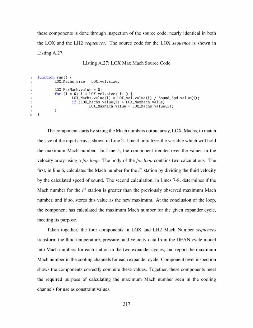
these components is done through inspection of the source code, nearly identical in both

the LOX and the LH2 sequences. The source code for the LOX sequence is shown in

Listing A.27.

Listing A.27: LOX Max Mach Source Code

1 function run() {2 LOX_Machs.size = LOX_vel.size;3

4 LOX_MaxMach.value = 0;5 for (i = 0; i < LOX_vel.size; i++) {6 LOX_Machs.value(i) = LOX_vel.value(i) / Sound_Spd.value(i);7 if (LOX_Machs.value(i) > LOX_MaxMach.value)8 LOX_MaxMach.value = LOX_Machs.value(i);9 }

10 }

The component starts by sizing the Mach numbers output array, LOX Machs, to match

the size of the input arrays, shown in Line 2. Line 4 initializes the variable which will hold

the maximum Mach number. In Line 5, the component iterates over the values in the

velocity array using a for loop. The body of the for loop contains two calculations. The

first, in line 6, calculates the Mach number for the ith station by dividing the fluid velocity

by the calculated speed of sound. The second calculation, in Lines 7-8, determines if the

Mach number for the ith station is greater than the previously observed maximum Mach

number, and if so, stores this value as the new maximum. At the conclusion of the loop,

the component has calculated the maximum Mach number for the given expander cycle,

meeting its purpose.

Taken together, the four components in LOX and LH2 Mach Number sequences

transform the fluid temperature, pressure, and velocity data from the DEAN cycle model

into Mach numbers for each station in the two expander cycles, and report the maximum

Mach number in the cooling channels for each expander cycle. Component level inspection

shows the components correctly compute these values. Together, these components meet

the required purpose of calculating the maximum Mach number seen in the cooling

channels for use as constraint values.

317

A.6.2 Pressure RMSE.

The Pressure RMSE component is a copy of the root mean square error analysis used

in the Pressure Profile Converger (see Section A.2.3.2 for complete modeling details). It

is included in the Constraints block to calculate an updated evaluation of the quality of the

extimated pressure profiles in the two expander cycles. These values are calculated at the

end of the overall system level simulation to provide a cross check for the estimated values

computed by the Pressure Profile Converger.

A.6.3 Chamber Mach Number.

The purpose of the Chamber Mach Number component is to calculate the Mach

number inside the combustion chamber. Chamber Mach numbers typically range between

Mach 0.1 and Mach 0.6, with values of Mach 0.1 indicating more conservative designs.

Smaller engines generally have lower chamber Mach numbers [5]. The component was

verified through inspection of its source code.

The Chamber Mach Number component uses a relationship between the engine’s

contraction ratio, the ratio of the chamber’s average cross-sectional are to the throat area,

and the chamber Mach number. Equation (A.72) shows this relationship.

Ac

At=

1M

[(2

γ + 1

) (1 +

γ − 12

M2)] γ+1

2(γ−1)

(A.72)

Note the chamber Mach number, M, appears as an inverse and a quadratic term,

complicating the process of solving for the chamber Mach number symbolically. However,

rearranging Equation (A.72) into a difference yields Equation (A.73). This relationship has

a root greater than zero and can be solved with the secant method. The Chamber Mach

Number component uses this approach to solve for the chamber Mach number as is shown

in Listing A.28.

1M

[(2

γ + 1

) (1 +

γ − 12

M2)] γ+1

2(γ−1)

−Ac

At= 0 (A.73)

318

Listing A.28: Chamber Mach Number Source Code

1 function run() {2 // set up secant method3 var x1 = 0.01;4 var x2 = 0.02;5 var x3 = 0.0;6 delta.value = 1;7

8 while (Math.abs(delta.value) > 0.01) {9 x3 = x2 - (calculateDelta(x2)/calculateDeltaPrime(x1, x2));

10 delta.value = calculateDelta(x3);11 x1 = x2;12 x2 = x3;13 }14

15 MachNumber.value = x3;16 }17

18 function calculateDelta(M) {19 var g = gamma.value;20 var AR = ChamberRatio.value;21

22 // break equation into parts to simplify coding23 // this is Eqn 5.37 in SPAD24 var a = 2 / (g + 1);25 var b = 1 + (g - 1) * Math.pow(M,2) / 2;26 var c = (g + 1) / (2 * (g - 1));27

28 return Math.pow(a*b,c) / M - AR;29 }30

31 function calculateDeltaPrime(M1, M2) {32 return (calculateDelta(M1) - calculateDelta(M2)) / (M1 - M2);33 }

Lines 2 - 15 implement the secant root finding method. The critical block of code is the

function calculateDelta which takes a single parameter, the guessed value for the chamber

Mach number, and returns the value of the calculation corresponding to Equation (A.73).

This function starts by assigning component level input variables to local variables on

Lines 19 and 20. The function then breaks the calculation of the difference between the

contraction ratio and the remaining terms into three small calculations on lines 24 - 26.

Line 24 calculates the 2γ+1 term and Line 25 calculates the 1 +

γ−12 M2 term. Finally, Line

26 calculates the overall exponent γ+12(γ−1) . The difference is then easily calculated by raising

the multiple of a and b to the c power, dividing by M, and subtracting the contraction ratio,

319

as is seen in Line 28. The remaining code uses the calculateDelta function to compute the

derivative using a secant approximation.

As can be seen above, the Chamber Mach Number component correctly calculates the

required value, and therefore the component meets its purpose.

A.6.4 Sanity Checks.

The purpose of the Sanity Checks component is to calculate the remaining system

level constraint values. These remaining constraint values are the total thickness of the

aerospike compared walls compared to the areospike’s radius at each station, the pressure

drop across the injector face for the oxidizer and the fuel expander cycles, the difference

between the chamber and aerospike radii at the throat, and the chamber’s outer radius

including wall thicknesses. The aerospike wall thickness is constrained unlike the chamber

because the aerospike grows inward and physically cannot exceed the aerospike radius at

any point along the nozzle. The injector face pressure drops are constrained by historical

data which indicates the values should be greater than 20%. Note, some systems go as

low as 5% and throttled engines generally have pressure drops of approximately 30% [5].

Given this range, the DEAN system level model uses values less than 10% and greater than

40% as constraint boundaries for the pressure drops across the injector face. The difference

between the outer and inner radii at the throat must be enforced to ensure it does not impact

operation of the engine. The inner and outer throat radii specify the throat area, and changes

to the throat area impact operation by leading to changes in the chamber pressure, thrust,

and specific impulse. Assuming a manufacturing tolerance for the radii at the throat of

0.001 in, a minimum value for the difference in throat radii of 0.1 in will limit the error in

the throat area to 2.0% Finally, the outer chamber radius is computed to ensure the DEAN

conforms to mission specific size constraints. The Sanity Checks component was verified

by inspection.

320

Listing A.29: Sanity Checks Source Code

1 sub run2 ’The goal of this script is to check geometry for inconsistencies3

4 fuel_length = LH2_radii.length5 H2_violate.length = LH2_radii.length6

7 ’This code checks each station to verify the cooling jacket thickness plus8 ’the cooling channel height plus the structural jacket thickness9 ’is less than the aerospike radius at every station

10

11 for fuel_counter = 0 to fuel_length - 112 If H2_h(fuel_counter) + cooltopspike_thickness(fuel_counter)13 + LH2_channel_thickness + SJspike_thickness14 > LH2_radii(fuel_counter) Then15 H2_violate(fuel_counter) = "fail"16 else17 H2_violate(fuel_counter) = "pass"18 End If19

20 if ( H2_violate(fuel_counter) = "fail" ) then21 location = "SanityChecks"22 msg = "The aerospike thickness exceeds aerospike radius"23 Err.raise vbError+1, location, msg24 end if25 next26

27

28 ’ This bit of code checks to make sure the injector pressure drop is between29 ’ 10 and 40% of the chamber pressure30 Plow_check = 0.1 * P0 ’Pressure drop should be more than 10% of chamber P31 Phigh_check = 0.4 * P0 ’Pressure drop should be less than 40% of chamber P32 Ox_Injector_P_Drop_Condition = "pass"33 Fuel_Injector_P_Drop_Condition = "pass"34

35 if Ox_pre_Injector_pressure - P0 < Plow_check then36 Ox_Injector_P_Drop_Condition = "fail"37 end if38 if Ox_pre_Injector_pressure - P0 > Phigh_check then39 Ox_Injector_P_Drop_Condition = "fail"40 end if41

42 if Fuel_pre_Injector_pressure - P0 < Plow_check then43 Fuel_Injector_P_Drop_Condition = "fail"44 end if45 if Fuel_pre_Injector_pressure - P0 > Phigh_check then46 Fuel_Injector_P_Drop_Condition = "fail"47 end if48

49 Ox_Injector_P_Drop = (Ox_pre_Injector_pressure - P0) / P050 Fuel_Injector_P_Drop = (Fuel_pre_Injector_pressure - P0) / P051

52 ’ calculate DeltaR_Throat53 DeltaR_Throat = LOX_radii(5) - LH2_radii(5)54

55 ’ calculate chamber outer radius located at base of engine56 Chamber_Outer_Radius = LOX_radii(0) + Chamber_Thickness(0)

321

57

58 end sub

Listing A.29 above contains the source code for the Sanity Checks component. The

first calculation compares the total thickness of the aerospike cooling and structural jackets

to the radius of the aerospike at every station along the length of the nozzle, Lines 11 -

25. The component uses a for-loop to iterate over the aerospike stations and compare the

total thickness (calculated by summing the cooling channel height, the cooling channel

thickness, the cooling channel top thickness, and the structural jacket thickness) to the

radius of the aerospike. In Lines 12 - 14, the first if statement implements the test for

the total thickness versus the aerospike radius. If the test condition is true, the thickness

exceeds the radius at the current station, and the test fails, otherwise it passes for this station,

and the iteration continues. The second if statement, shown in Line 20, throws an exception

when the test fails, causing the model execution to be halted, and the current design point

to be treated as a failed run, which ModelCenter treats as an invalid design since it includes

unbuildable geometry.

The second calculation compares the pressure drops at the injector faces to expected

values by comparing the difference between the pre-injector pressure and the chamber

pressure to the low and high pressure drop limits, 10% and 40% of chamber pressure

respectively. Lines 35 - 40 implement the pressure drop calculation for the LOX expander

cycle. The same process is used for the LH2 cycle in Lines 42 - 47. The last block of

code in Lines 49 - 50 report the pressure drops as a percentage so they can be used by the

ModelCenter Optimization Tool as constraint values to guide optimization studies toward

designs which fall in the expected range of pressure drops.

The third calculation computes the difference between the outer and inner radii at

the throat (DeltaR Throat). Line 53 implements this calculation by taking the difference

between the chamber and aerospike radii at the throat. The last calculation computes the

322

chamber outer radius (Chamber Outer Radius) in Line 56. This calculation is a simple

summation of the radius of the chamber cooling channel at the base of the engine and the

thickness of the chamber wall at the base of the engine.

The analysis above shows the component correctly detects DEAN designs with

infeasible aerospike structures, correctly calculates the pressure drops across the injector

face for the two expander cycles as well as the difference between the outer and inner radii

at the throat and the outer chamber radius. These calculations constitute the remaining

system level constraints, validating this component.

A.7 Conclusion

The results of this appendix verify and validate the individual analysis modules in the

fourth generation DEAN model. The inspection of the source code for each component

confirms the implementation and underlying engineering assumptions. Tests of critical

analyses including the calculation of the aerospike contour and the estimation of the pump

pressure ratios further demonstrate the correct function of the analysis modules. Finally,

comparisons of each module’s results to its purpose validate the module’s inclusion in the

system level DEAN model.

323

Appendix B: Revisiting Previous Results with the Fourth Generation DEAN Model

The three designs from previous DEAN research were reevaluated using the fourth

generation DEAN model to confirm the results of earlier research. For each design, the

system level design variables were entered into the updated DEAN model and then the

model was run to calculate the engine performance.

Several of the system level design variables are common to all three designs. These

design variables represent system level assumptions in the model and are listed in Table

B.1.

Table B.1: Shared Design Variable Values for Model Comparisons

Variable Value




Percent Weight of Hardware 5%

Cowl Length 0.1





The first generation DEAN design, developed by Martin, predates any of the

parameterizations of the DEAN model. It also predates the architecture update of routing

all of the fuel flow through the cooling channels. In Martin’s design, only half of the

fuel flow was routed through the cooling channels. As such, its design variables must be

324

recomputed. Table B.2 lists the values for the design variables and the source for each

value.

Table B.2: Design Variable Values for Generation 1 DEAN Model

Variable Value Source

Expansion Ratio 4.94 ε = Ae/At = π(52)/15.9

Throat Area (in2) 15.9 Gen 1 DEAN Model

Chamber Length (in) 24 Gen 1 DEAN Model

Characteristic Length (in) 126.5 Manual Testing

Vacuum Thrust (lbf) 57,231 Gen 1 DEAN Results

Oxidizer-to-Fuel Ratio 7.0 Gen 1 DEAN Model

Chamber Throat AR 3.0 Gen 1 DEAN Model

Chamber Stations Adjustment 0.95 Manual Testing

Chamber Station 5 Adjustment 1.11 Manual Testing

Chamber Cooling Channels Ratio 25.0 Manual Testing

Nozzle Throat AR 0.57 Gen 1 DEAN Model

Nozzle Station 1 Adjustment 13.0 Manual Testing

Nozzle Station Spike Adjustment 2.33 Manual Testing

Aerospike Cooling Channels Ratio 11.2 Manual Testing

Chamber Structural Jacket Material Aluminum 7075-T6 Martin’s Thesis

Chamber Cooling Jacket Material Silicon Carbide Martin’s Thesis

Aerospike Structural Jacket Material Silicon Carbide Manual Testing

Aerospike Cooling Jacket Material Aluminum 7075-T6 Manual Testing

Aerospike Tip Material Niobium Martin’s Thesis

325

The first attempt to run Martin’s design failed to converge on working cooling channel

thicknesses in the aerospike. Martin selected copper for the aerospike material, however,

the copper was being overheated (for some cases it was reaching over 500% of its melting

point). The aerospike materials were updated to match the chamber materials to resolve

this error. Additionally, a number of adjustments were required to Martin’s design point

as documented to adapt it to fit the parameterizations in the revised DEAN model. For

example, the calculating the characteristic length from Martin’s other design values does

not yield the correct internal chamber geometry. This discrepancy is caused by the

approximations used in calculating the internal geometry from the system level design

variables. Similarly, the aerospike cooling channel geometry had to be corrected to account

for the increased mass flow of running all of the LH2 through the cooling channels. These

updated values were found using manual testing.

The results of the comparison for the first generation DEAN design are summarized

in Table B.3. Two of the results are worth reviewing. First, many of the values are

very close matches between the two models, with a few key exceptions. For example,

the reported value for the specific impulse is significantly lower in the fourth generation

model. This result is due to the findings from Hall’s research which indicate the expansion

ratio should be calculated from the aerospike geometry instead of using an assumed value

such as Martin’s expansion ratio of 125. Likewise, the chamber pressure, mass flow, and

LH2 pump power are higher in the new model. These increased values are driven by the

architecture change between Martin’s model and later research which feeds all of the LH2

through the cooling channels instead of feeding half of the LH2 through a bypass around

the cooling chamber and LH2 turbine. Finally, the fourth generation model gives a much

lower weight, however this is to be expected with the change in materials required to get

the model to run to completion.

326

Second, as mentioned above, Martin’s material selection does not converge in the

revised model. This result is driven by a difference in assumptions between Martin’s

research and the revised model. In Martin’s research, the cooling channel wall thickness

is simply assumed to be 0.02 in and does not include any structural analysis, whereas

the current model sizes the cooling channel wall thickness based on the pressure in the

cooling channels and the material strength for the cooling channel material at its current

temperature. This additional sizing code can, under high channel pressures, experience a

divergent cycle where the wall thickness grows to accommodate the channel pressure which

leads to increased wall temperature, which leads to lower material strength, which in turn

leads to even greater wall thickness. This cycle continues until the model times out. This

behavior explains the need to change the aerospike material selection, as the copper from

Martin’s design was not able to withstand the pressures and temperatures in the cooling

channels at only 0.02 in thick.

As can be seen in Figure B.1 the agreement between the two models continues with the

rendered geometry. The wall thicknesses from the structural sizing codes are in proportion

to the manually computed wall sizes from Martin’s work. And the aerospike nozzle

approximation is also a good match for the nozzle modeled by Martin.

327

Table B.3: Results of Generation 1 DEAN Design Comparison

Variable Original Value[2] Updated Value Delta

Vacuum Specific Impulse (s) 472.7 412.9 -12.7%

Thrust-to-Weight Ratio 119.0 138.6 16.5%

Chamber Pressure (psia) 1739 1999 15.0%

Chamber Temperature (R) 6586 6630 0.7%

Total Mass Flow (lbm/s) 121.1 138.6 14.5%

Maximum Mach Number, LOX 0.57 0.48 -15.8%

Maximum Mach Number, LH2 0.67 0.74 10.4%

Chamber Wall Temp (% Melt Point) - 65.5 -

Aerospike Wall Temp (% Melt Point) - 69.5 -

Injector Face Pressure Drop, LOX (%) - 23.8 -

Injector Face Pressure Drop, LH2 (%) - 17.6 -

Required Power for LOX Pump (HP) 2587 2591 0.2%

Required Power for LH2 Pumps (HP) 3573 4562 27.7%

∆rthroat (in) 0.5 0.53 6.0%

Engine Length (in) 38 36.3 4.5%

Outer Chamber Radius (in) - 6.8 -

328

(a) Published Geometry, credit D.

Martin[2]

(b) Rendered Geometry

Figure B.1: Geometry Comparison for First Generation DEAN Design

Like the first generation DEAN design, the second generation design point predates

many of the current parameterizations of the DEAN model. As such, several of its design

variables also had to be recomputed. Table B.4 lists the values for the design variables and

the source for each value. The materials selection followed those used in the Martin design

point as the second generation model’s design is a scaling of Martin’s design.

The results of the comparison for the second generation DEAN design are summarized

in Table B.5. Note, the second generation DEAN model did not include any structural

sizing analyses, so its results do not include weight related values. There are three

significant results from this comparison. First, as with the results for first generation

DEAN design point, the results showed the updated model yields a much lower specific

impulse than the previous models do. As before, this is due to the change in the modeling

assumption for the expansion ratio first made by Hall.

Second, the maximum Mach number for the LH2 cycle was quite different between

the two models. Recall, the second generation DEAN model used a static set of values

for the pressure profile guesses in the two expander cycles. This decision was an artifact

329




Throat Area (in2) 18.9 Gen 2 DEAN Results

Chamber Length (in) 14.25 Gen 2 DEAN Model

Characteristic Length (in) 51.3 L∗ = Vc/At = 970.0/18.9

Vacuum Thrust (lbf) 50,900 Gen 2 DEAN Results



Chamber Stations Adjustment 0.95 Manual Testing

Chamber Station 5 Adjustment 1.11 Manual Testing



Nozzle Station 1 Adjustment 13.0 Manual Testing

Nozzle Station Spike Adjustment 2.33 Manula Testing


Chamber Structural Jacket Material Aluminum 7075-T6 Martin’s Thesis

Chamber Cooling Jacket Material Silicon Carbide Martin’s Thesis

Aerospike Structural Jacket Material Silicon Carbide Manual Testing

Aerospike Cooling Jacket Material Aluminum 7075-T6 Manual Testing

Aerospike Tip Material Niobium Martin’s Thesis

from Martin’s original model. The revised model calculates these guesses based on the

current design point. The cooling channel pressure levels, and in turn the maximum

Mach numbers, depend greatly on these guessed pressure levels. The significant difference

between the dynamically generated values and Martin’s static values in the LH2 cycle led

330

to vastly different solutions for the actual pressure profiles which yielded very different

Mach numbers.

Finally, the original research in the second generation DEAN predates calculations for

the thrust-to-weight ratio, and therefore had to make assumptions about the impact of its

proposed design changes on the thrust-to-weight ratio. The updated DEAN model yielded

a thrust-to-weight ratio 194.1 for second generation design, an improvement of 63% over

the first generation DEAN results. Clearly this design achieved the desired result of further

optimizing the DEAN with respect to the engine’s thrust-to-weight ratio.

Figure B.2 shows the rendered geometry for the second generation DEAN design.

There was no previously published geometry to compare the rendering to as there was no

automated rendering available in the second generation model.

Figure B.2: Geometry for Second Generation DEAN Design

331




Thrust-to-Weight Ratio - 194.1 -


Chamber Temperature (R) 6413 6440 0.4%

Total Mass Flow (lbm/s) 104 120.4 15.8%

Maximum Mach Number, LOX 0.37 0.46 24.3%

Maximum Mach Number, LH2 0.96 0.46 -52.1%

Chamber Wall Temp (% Melt Point) - 57.1 -

Aerospike Wall Temp (% Melt Point) - 35.0 -



Required Power for LOX Pump (HP) 1053 1333 26.6%

Required Power for LH2 Pumps (HP) 3847 3688 -4.1%

∆rthroat (in) 0.58 0.64 10.3%

Engine Length (in) 27.9 26.0 -6.8%


332

The third generation DEAN design, developed by J. Hall, was the first to incorporate

structural sizing for the cooling and structural jackets in the model’s automated design loop.

The initial drafts of the fourth generation DEAN model included the same sizing code as

Hall’s model. However, the code review conducted during the verification process revealed

anomalies in Hall’s structural sizing codes which led to over sized components. Addressing

the anomalies led to updates to the sizing codes for both the cooling and structural jackets.

These updates were expected to result in lighter weight designs. Hall’s model was also the

model with the closest parameterization to the current research. As such, most of the values

for the design variables can be sourced directly from his model and analysis. One key set

of values was missing from this documentation: the number of cooling channels in both

expander cycles. Trade studies were run to find values which yielded similar maximum

Mach numbers. Table B.6 lists the values for the design variables and the source for each

value.

The results of the comparison for the third generation DEAN design are summarized in

Table B.7. The fourth generation DEAN model was able to capture a design based on Hall’s

work which was quite close to his results. The key difference occured in the values related

to the thrust-to-weight ratio and the power required for the pumps. The improved thrust-to-

weight ratio is driven by a weight savings of nearly 49 lbf, with a corresponding increase

in the thrust-to-weight ratio. This difference in weight was driven by three factors. First,

the chamber cooling channels had far lower pressures which result in a thinner wall for the

chamber structural jacket. Second, the differences in the structural sizing codes between

the third and fourth generation models included changes which yielded less conservative

estimates for wall thicknesses, leading to thinner walls in both structural jackets. Third,

the fourth generation model gave a significantly lower power required for both the LOX

and LH2 pumps, which resulted in weight savings. The power savings for the pumps was

333




Throat Area (in2) 18.0 Gen 3 DEAN Model

Chamber Length (in) 14.5 Gen 3 DEAN Model

Characteristic Length (in) 37.8 Gen 3 DEAN Model

Vacuum Thrust (lbf) 50,161 Gen 3 DEAN Model



Chamber Stations Adjustment 1.0 Gen 3 DEAN Model

Chamber Station 5 Adjustment 1.0 Gen 3 DEAN Model



Nozzle Station 1 Adjustment 1.0 Gen 3 DEAN Model

Nozzle Station Spike Adjustment 1.0 Gen 3 DEAN Model


Chamber Structural Jacket Material Aluminum 7075-T6 Gen 3 DEAN Model

Chamber Cooling Jacket Material Silicon Carbide Gen 3 DEAN Model

Aerospike Structural Jacket Material Oxygen-Free Copper Gen 3 DEAN Model

Aerospike Cooling Jacket Material Oxygen-Free Copper Gen 3 DEAN Model

Aerospike Tip Material Oxygen-Free Copper Gen 3 DEAN Model

driven by lower pressure ratios which resulted from a difference between the dynamically

generated values and the static values from the first generation model.

Three other results bear closer inspection. First, the values for the specific impulse

and the total mass flow are very similar between the two models. Both values are within

334

approximately 1% between the two models. This agreement indicates the custom nozzle

element used in the fourth generation DEAN model returns similar results to Hall’s more

complex TDK analysis. Second, Hall’s values for the maximum pressures in the cooling

channels are reported as approximations in the table since he reports these values in graphs

and not tabular form.




Thrust-to-Weight Ratio 142.2 163.9 15.3%


Chamber Temperature (R) - 6477 -

Total Mass Flow (lbm/s) 116.5 117.9 1.2%

Maximum Mach Number, LOX 0.21 0.33 52.4%

Maximum Mach Number, LH2 0.37 0.38 -2.7%

Chamber Wall Temp (% Melt Point) 58.6 59.7 1.9%

Aerospike Wall Temp (% Melt Point) 43.0 49.1 14.2%



Required Power for LOX Pump (HP) 1945 1442 -25.9%

Required Power for LH2 Pumps (HP) 3847 3340 -13.2%

∆rthroat (in) 0.61 0.61 0.0%

Engine Length (in) 26.7 26.4 -1.1%


335

As with the first generation design, Figure B.3 shows there is strong agreement

between the rendered geometry for the third generation design. The simplifications made

in the fourth generation model to support studying a wider trade space gave similar results

for both the chamber and the aerospike nozzle in the geometry rendering.

(a) Published Geometry, credit

J. Hall[4]

(b) Rendered Geometry

Figure B.3: Geometry Comparison for Third Generation DEAN Design

336

Bibliography

[1] Sloop, J., Liquid Hydrogen as a Propulsion Fuel, 1945-1959, National Aeronauticsand Space Administration, 1978.

[2] Martin, D. F., Computational Design of Upperstage Chamber, Aerospike, & CoolingJacket of Dual-Expander Rocket Engine, (MS Thesis, Air Force Institute ofTechnology), 2008.

[3] Huzel, D. and Huang, D., Modern Engineering for Design of Liquid-PropellantRocket Engines, AIAA, 1992.

[4] Hall, J., Optimized Dual Expander Aerospike Rocket, (MS Thesis, Air Force Instituteof Technology), 2010.

[5] Humble, R. W., Space Propulsion Analysis and Design, McGraw-Hill Inc, 1995.

[6] Clark, S., “ULA’s common upper stage engine to fly this year,” cited June, 2014.

[7] NASA, “Centaur upper stage being lifted.jpg (web page),” cited 06/25/2014.

[8] Donahue, B. and Sigmon, S., “The Space Launch System Capabilities with a NewLarge Upper Stage,” AIAA Space 2013 Conference & Exposition, AIAA, 2013.

[9] USAF, “X-37 Orbital Test Vehicle (web page),” cited 04/09/2014.

[10] Clark, S., “Inspections have begun on Air Force space plane (web page),” cited04/09/2014.

[11] “RL10B-2 Propulsion System,” Tech. rep., Pratt & Whitney Rocketdyne, 2009.

[12] Buzzell, J., “Testing for the J-2X Upper Stage Engine,” SpaceOps 2010 Conference,AIAA, 2010.

[13] NASA, “The J-2X Engine Fact Sheet,” cited 04/09/2014.

[14] Buttler, K., “AR2-3 Engine Refurbishment and Gas Generator Testing,” 35thAIAA/ASME/SAE/ASEE Joint Propulsion Conference and Exhibit: 20-23 June, 1998,AIAA, 1999.

[15] Hammond, W., Design Methodologies for Space Transportation Systems, AIAA,2001.

[16] DoD, “Defense Budget Priorities and Choices Fiscal Year 2014,” cited 06/20/2014.

[17] Center/DD., L., “AFDD 3-14 Space Operations,” cited 06/20/2014.

337

[18] Command, A. F. S., “Next Generation Engine (NGE) Request for Information (webpage),” cited 12/06/2011.

[19] DeGeorge, D. and Fletcher, S., “The Integrated High Payoff Rocket PropulsionTechnology Program and Tactical Missile Propulsion Status,” Tech. Rep. AFRL-PR-EN-TP-2002-214, US Air Force, Air Force Research Laboratory, 2002.

[20] Dumbacher, D., “The Development of the X-37 Re-Entry Vehicle,” 55th InternationalAstronautical Congress, AIAA, 2004.

[21] Pienkowski, J., Whitmore, S., and Spencer, M., “Analysis of the AerodynamicOrbital Transfer Capabilities of the X-37 Space Maneuvering Vehicle (SMV),” 41stAerospace Sciences Meeting and Exhibit, AIAA, 2003.

[22] Singer, J., Cook, J., and Singer, C., “NASA Space Launch System OperationsStrategy,” SpaceOps 2012 Conference, AIAA, 2012.

[23] Mc Hugh, B., “Numerical Analysis of Existing Liquid Rocket Engines as aDesign Process Starter,” 31st AIAA/ASME/SAE/ASEE Joint Propulsion Conferenceand Exhibit: 10 - 12 July 1995, AIAA, San Diego, CA, 1995.

[24] Sutton, G. P., Rocket Propulsion Elements, Eighth Edition, John Wiley & Sons Inc,2010.

[25] Arguello, A. A., The Concept Design of a a Split Flow Liquid Hydrogen Turbopump,(MS Thesis, Air Force Institute of Technology), 2008.

[26] Strain, W. S., Design of an Oxygen Turbopump for a Dual Expander Cycle RocketEngine, (MS Thesis, Air Force Institute of Technology), 2008.

[27] Simmons, J. and Branam, R., “Parametric Study of Dual-Expander Aerospike NozzleUpper Stage Rocket Engine,” AIAA Journal of Spacecraft and Rockets, Vol. 48, No. 2,2011, pp. 355–367.

[28] Wiesel, W. E., Spaceflight Dynamics, Second Edition, McGraw-Hill, 1997.

[29] REDTOP-LITE version 1.85 User’s Guide, SpaceWorks Software, Atlanta, GA, 2011.

[30] RPA User Manual, 2011.

[31] NPSS v1.6.4 User Guide, NASA Glenn Research Center, Cleveland, OH, 2006.

[32] NPSS v1.6.4 Rockets Supplement, NASA Glenn Research Center, Cleveland, OH,2006.

[33] Binder, M., “An RL10A-3-3A Rocket Engine Model Using the Rocket Engine Tran-sient Simulator (ROCETS) Software,” AIAA/SAE/ASME/ASEE 29th Joint PropulsionConference and Exhibit: June 28-30, 1993, AIAA, Monterey, CA, 1993.

338

[34] Bond, P., editor, Jane’s Space Systems and Industry 2011 - 2012, Jane’s InformationGroup Limited, 2011.

[35] “RL10A-4 Propulsion System,” Tech. rep., Pratt & Whitney Rocketdyne, 2009.

[36] Baker, D., editor, Jane’s Space Directory 2006 - 2007, Jane’s Information GroupLimited, 2006.

[37] “NASA - Nano-Satellite Launch Challenge,” cited January, 2011.

[38] Corporation, T. B., “X-37B Orbital Test Vehicle (web page),” cited 04/09/2014.

[39] Sutton, G., History of Liquid Propellant Rocket Engines, AIAA, 2006.

[40] Beichel, R., O’Brien, C., and Taylor, J., “Is There a Future in Liquid RocketPropulsion?” AIAA/SAE/ASME 27th Joint Propulsion Conference, AIAA, 1991.

[41] Nguyen, T., Hyde, J., and Ostrander, M., “Aerodynamic Performance Analysis ofDual-Fuel/Dual-Expander Nozzles,” AIAA/ASME/SAE/ASEE 24th Joint PropulsionConference, AIAA, 1988.

[42] Hagemann, G., Manski, D., and Kruille, G., “Dual Expander Engine FlowfieldSimulations,” 31st AIAA/ASME/SAE/ASEE Joint Propulsion Conference and Exhibit,AIAA, 1995.

[43] Froning, H. and Beichel, R., “Impact of dual fuel and dual expander rockets on RLVs,”AIAA Space Programs and Technologies Conference: 1996, AIAA, 1996.

[44] Buckmann, P., Shimp, N., Viteri, F., and Proctor, M., “Design and Test of an OxygenTurbopump For a Dual Expander Cycle Rocket Engine,” AIAA/ASME/SAE/ASEE 25thJoint Propulsion Conference, AIAA, 1989.

[45] Besnard, E. and Garvey, J., “Development and Flight-Testing of Liquid PropellantAerospike Engines,” 40th AIAA/ASME/SAE/ASEE Joint Propulsion Conference andExhibit, AIAA, 2004.

[46] Ladeinde, T. and Hsun, C., “Performance Comparison of a Full-Length anda Truncated Aerospike Nozzle,” 46th AIAA/ASME/SAE/ASEE Joint PropulsionConference & Exhibit, AIAA, 2010.

[47] Gross, K., “Performance Analysis of Aerospike Rocket Engines,” Tech. Rep. Techdoc19730004121, NASA, 1972.

[48] Angelino, G., “Approximate Method for Plug Nozzle Design,” AIAA Journal, Vol. 2,No. 10, 1964, pp. 1834–1835.

[49] Dunn, S. and Coats, D., “Nozzle Performance Predictions Using the TDK 97 Code,”33rd AIAA/ASME/SAE/ASEE Joint Propulsion Conference and Exhibit, AIAA, 1997.

339

[50] Wuye, D., Yu, L., Xianchen, C., and Haibin, T., “Aerospike Nozzle PerformanceStudy and its Contour Optimization,” 37th AIAA/ASME/SAE/ASEE Joint PropulsionConference and Exhibit, AIAA, 2001.

[51] Grieb, D. e. a., “Design and Analysis of a Reusable N2O-Cooled Aerospike Nozzlefor Labscale Hybrid Rocket Motor Testing,” 47th AIAA/ASME/SAE/ASEE JointPropulsion Conference and Exhibit, AIAA, 2011.

[52] O’Leary, R. and Beck, J., “Nozzle Design,” Threshold: Pratt&Whitney Rocketdyne’sengineering journal of power technology, Vol. Spring, 1992.

[53] Sackheim, R., “Overview of United States Space Propulsion Technology andAssociated Space Transportation Systems,” Journal of Propulsion and Power, Vol. 22,No. 6, 1992, pp. 1310–1333.

[54] Bui, T. e. a., “Flight Research of an Aerospike Nozzle Using High Power SolidRockets,” 41st AIAA/ASME/SAE/ASEE Joint Propulsion Conference and Exhibit,AIAA, 2005.

[55] Besnard, E. and Garvey, J., “Development and Flight-Testing of Liquid PropellantAerospike Engines,” 40th AIAA/ASME/SAE/ASEE Joint Propulsion Conference andExhibit, AIAA, 2004.

[56] Besnard, E. and Garvey, J., “Aerospike Engines for Nanosat and Small LaunchVehicles (NLV/SLV),” Space 2004 Conference and Exhibit, AIAA, 2004.

[57] Corporation, T. B., “Annular-Aerospike.jpg (web page),” cited 06/25/2014.

[58] NASA, “Twin Linear Aerospike XRS-2200 Engine PLW edit.jpg (web page),” cited06/25/2014.

[59] Garvey, K., “Aerospike close-up.jpg (web page),” cited 06/25/2014.

[60] ModelCenter 10.2 User Manual, Phoenix Integration, Blacksburg, VA, 2013.

[61] Moen, M., Methane Dual Expander Aerospike Nozzle Rocket Engine, (MS Thesis,Air Force Institute of Technology), 2012.

[62] Rao, S., Engineering Optimization: Theory and Practice, John Wiley & Sons, fourthedition ed., 2009.

[63] Minick, A. and Peery, S., “Design and Development of an Advanced Liquid HydrogenTurbopump,” 34th AIAA/ASME/SAE/ASEE Joint Propulsion Conference and Exhibit:13-15 July, 1998, AIAA, 1998.


[65] “Thermophysical Properties of Fluid Systems,” cited May 27, 2010.

340

[66] Krach, A. E. and Sutton, A. M., “Another Look at the Practical and TheoreticalLimits of an Expander Cycle, LOX/H2 Engine,” 35th AIAA/ASME/SAE/ASEE JointPropulsion Conference and Exhibit: 20-24 June, 1999, AIAA, 1998.


[68] Atlas V Launch Services User’s Guide, March 2010, United Launch Alliance, 2010.

[69] Delta IV Launch Services User’s Guide, June 2013, United Launch Alliance, 2013.

[70] Shigley, J. and Mischke, C., Mechanical Engineering Design, McGraw-Hill, fifthedition ed., 1989.

[71] Stewart, J., Calculus: Concepts and Contexts, Second Edition, Wadsworth Group,Brooks/Cole, Thomson Learning, 2001.

341

REPORT DOCUMENTATION PAGE Form ApprovedOMB No. 0704–0188

The public reporting burden for this collection of information is estimated to average 1 hour per response, including the time for reviewing instructions, searching existing data sources, gathering andmaintaining the data needed, and completing and reviewing the collection of information. Send comments regarding this burden estimate or any other aspect of this collection of information, includingsuggestions for reducing this burden to Department of Defense, Washington Headquarters Services, Directorate for Information Operations and Reports (0704–0188), 1215 Jefferson Davis Highway,Suite 1204, Arlington, VA 22202–4302. Respondents should be aware that notwithstanding any other provision of law, no person shall be subject to any penalty for failing to comply with a collectionof information if it does not display a currently valid OMB control number. PLEASE DO NOT RETURN YOUR FORM TO THE ABOVE ADDRESS.

1. REPORT DATE (DD–MM–YYYY) 2. REPORT TYPE 3. DATES COVERED (From — To)

4. TITLE AND SUBTITLE 5a. CONTRACT NUMBER

5b. GRANT NUMBER

5c. PROGRAM ELEMENT NUMBER

5d. PROJECT NUMBER

5e. TASK NUMBER

5f. WORK UNIT NUMBER

6. AUTHOR(S)

7. PERFORMING ORGANIZATION NAME(S) AND ADDRESS(ES) 8. PERFORMING ORGANIZATION REPORTNUMBER

9. SPONSORING / MONITORING AGENCY NAME(S) AND ADDRESS(ES) 10. SPONSOR/MONITOR’S ACRONYM(S)

11. SPONSOR/MONITOR’S REPORTNUMBER(S)

16. SECURITY CLASSIFICATION OF:

a. REPORT b. ABSTRACT c. THIS PAGE

17. LIMITATION OFABSTRACT

18. NUMBEROFPAGES

19a. NAME OF RESPONSIBLE PERSON

19b. TELEPHONE NUMBER (include area code)

Standard Form 298 (Rev. 8–98)Prescribed by ANSI Std. Z39.18

18–09–2014 Doctoral Dissertation Jun 2009–Sep 2014

Design and Evaluation of Dual-Expander Aerospike Nozzle Upper StageEngine

Simmons, III, Joseph R.,

Air Force Institute of TechnologyGraduate School of Engineering and Management (AFIT/EN)2950 Hobson WayWPAFB, OH 45433-7765

AFIT-ENY-DS-14-S-06

Intentionally Left Blank

N/A

N/A

12. DISTRIBUTION / AVAILABILITY STATEMENTDISTRIBUTION STATEMENT A:APPROVED FOR PUBLIC RELEASE; DISTRIBUTION UNLIMITED13. SUPPLEMENTARY NOTESThis work is declared a work of the U.S. Government and is not subject to copyright protection in the United States.14. ABSTRACTThe goal of the Dual-Expander Aerospike Nozzle, a modification to traditional engine architectures, is to find thosemissions and designs for which it has a competitive advantage over traditional upper stage engines such as the RL10.Previous work focused on developing an initial design to demonstrate the feasibility of the Dual-Expander AerospikeNozzle. This research expanded the original cycle model in preparation for optimizing the engine’s specific impulse andthrust-to-weight ratio. The changes to the model allowed automated parametric and optimization studies. Preliminaryparametric studies varying oxidizer-to-fuel ratio, total mass flow, and chamber length showed significant improvements.Drawing on modeling lessons from previous research, this research devloped a new engine simulation capable of achievinga specific impulse comparable to the RL10. Parametric studies using the new model verified the Dual-ExpanderAerospike Nozzle architecture conforms to rocket engine theory while exceeding the RL10’s performance. Finally, thisresearch concluded by optimizing the Dual-Expander Aerospike Nozzle engine for three US government missions: theNext Generation Engine program, the X-37 mission, and the Space Launch System. The optimized Next GenerationEngine design delivers 35,000 lbf of vacuum thrust at 469.4 seconds of vacuum specific impulse with a thrust-to-weightratio of 127.2 in an engine that is one quarter the size of a comparable RL10. For the X-37 mission, the optimized designoperates at 6,600 lbf of vacuum thrust and has a vacuum specific impulse of 457.2 seconds with a thrust-to-weight ratioof 107.5. The Space Launch System design produces a vacuum thrust of 100,000 lbf with a vacuum specific impulse of465.9 seconds and a thrust-to-weight ratio of 110.2. When configured in a cluster of three engines, the Dual-ExpanderAerospike Nozzle matches the J2-X vacuum thrust with a 4% increase in specific impulse while more than doubling theJ2-X’s thrust-to-weight ratio.15. SUBJECT TERMSdual-expander, upper stage, NGE, aerospike, optimization, rocket propulsion

U U U UU 376

Dr. Jonathan Black (ENY)

(937) 255-3636 x0000 [email protected]

design and evaluation of dual-expander aerospike nozzle

Documents