numerical analysis of aerospike engine nozzle performance

International Journal of Aviation, International Journal of Aviation,

Aeronautics, and Aerospace Aeronautics, and Aerospace

Volume 8 Issue 2 Article 12

2021

Numerical Analysis of Aerospike Engine Nozzle Performance at Numerical Analysis of Aerospike Engine Nozzle Performance at

Various Truncation Lengths Various Truncation Lengths

Sam Dakka Dr The University of Nottingham, [email protected] Oliver Dennison [email protected]

Follow this and additional works at: https://commons.erau.edu/ijaaa

Part of the Aerodynamics and Fluid Mechanics Commons, Propulsion and Power Commons, and the

Space Vehicles Commons

Scholarly Commons Citation Scholarly Commons Citation Dakka, S., & Dennison, O. (2021). Numerical Analysis of Aerospike Engine Nozzle Performance at Various Truncation Lengths. International Journal of Aviation, Aeronautics, and Aerospace, 8(2). https://doi.org/10.15394/ijaaa.2021.1601

This Article is brought to you for free and open access by the Journals at Scholarly Commons. It has been accepted for inclusion in International Journal of Aviation, Aeronautics, and Aerospace by an authorized administrator of Scholarly Commons. For more information, please contact [email protected].

http://commons.erau.edu/

http://commons.erau.edu/

https://commons.erau.edu/ijaaa

https://commons.erau.edu/ijaaa

https://commons.erau.edu/ijaaa/vol8

https://commons.erau.edu/ijaaa/vol8/iss2

https://commons.erau.edu/ijaaa/vol8/iss2/12

https://commons.erau.edu/ijaaa?utm_source=commons.erau.edu%2Fijaaa%2Fvol8%2Fiss2%2F12&utm_medium=PDF&utm_campaign=PDFCoverPages

http://network.bepress.com/hgg/discipline/222?utm_source=commons.erau.edu%2Fijaaa%2Fvol8%2Fiss2%2F12&utm_medium=PDF&utm_campaign=PDFCoverPages



https://doi.org/10.15394/ijaaa.2021.1601

https://doi.org/10.15394/ijaaa.2021.1601

mailto:[email protected]

Numerical Analysis of Aerospike Engine Nozzle Performance at Various Numerical Analysis of Aerospike Engine Nozzle Performance at Various Truncation Lengths Truncation Lengths

Cover Page Footnote Cover Page Footnote The research received no external funding. The research was conducted in the frame work of Oliver Dennison Engineering Degree at the University of Nottingham

This article is available in International Journal of Aviation, Aeronautics, and Aerospace: https://commons.erau.edu/ijaaa/vol8/iss2/12



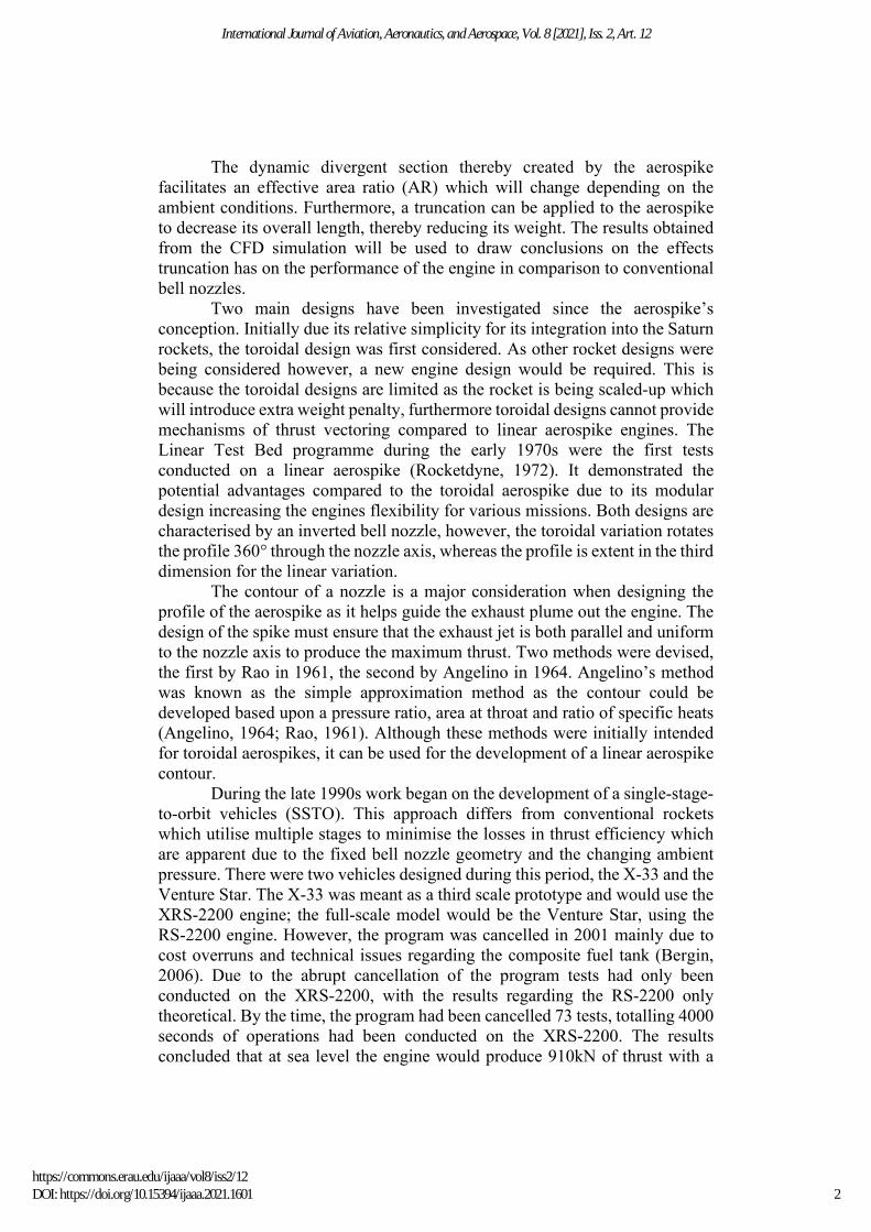
The design of rocket nozzles has not significantly changed since the bell nozzle contour was first detailed by Rao in 1958. To obtain the maximum thrust, the exhaust gases must be completely expanded to the ambient pressure while ensuring the nozzle contour provides a parallel uniform jet at the exit. This can be expressed by: 𝐹𝐹 = �̇�𝑚𝑉𝑉𝑒𝑒 + (𝑃𝑃𝑒𝑒 − 𝑃𝑃𝑎𝑎𝑎𝑎𝑎𝑎)𝐴𝐴𝑒𝑒 (1) This relationship demonstrates how the thrust is related to the ambient pressure and highlights the issue regarding the efficiency of bell nozzles at different altitudes. If the ambient pressure is greater than the exhaust exit pressure, the flow is said to be over-expanded resulting in a reduction in thrust due oblique shock waves and flow separation inside the bell-shaped nozzle. This particularly applies at altitudes close to sea-level due to the higher ambient pressures found, therefore, there will be a reduction in efficiency. Furthermore, as the bell nozzle is a fixed geometry, the design of the contour will be based upon one altitude at which it will produce the optimum thrust. However, at differing altitudes, the maximum thrust will decrease due to the changing ambient pressure. The design of the aerospike engine ensures that the decreasing ambient pressure associated with an increasing altitude will not greatly reduce its performance up to its design altitude. This is due to the boundary formed by the ambient pressure on the exhaust gases, in comparison a bell nozzle has a physical boundary. By using the ambient pressure to form the boundary, it is free to change depending on the ambient conditions. Figure1 demonstrates the differences in the exhaust gases between an aerospike nozzle design and a bell nozzle design at different stages in flight. Figure 1 Exhaust Plume with Changing Altitude

Note. From “Breakthroughs in Engine Propulsion Research with High-Performance Computing,” by L. Bravo and M. Ihme, 2017, DSIAC Journal, 4(4), 1–39.

1

Dakka and Dennison: Numerical Analysis of Aerospike Engine Nozzle Performance at Various Truncation Lengths

Published by Scholarly Commons, 2021

The dynamic divergent section thereby created by the aerospike facilitates an effective area ratio (AR) which will change depending on the ambient conditions. Furthermore, a truncation can be applied to the aerospike to decrease its overall length, thereby reducing its weight. The results obtained from the CFD simulation will be used to draw conclusions on the effects truncation has on the performance of the engine in comparison to conventional bell nozzles. Two main designs have been investigated since the aerospike’s conception. Initially due its relative simplicity for its integration into the Saturn rockets, the toroidal design was first considered. As other rocket designs were being considered however, a new engine design would be required. This is because the toroidal designs are limited as the rocket is being scaled-up which will introduce extra weight penalty, furthermore toroidal designs cannot provide mechanisms of thrust vectoring compared to linear aerospike engines. The Linear Test Bed programme during the early 1970s were the first tests conducted on a linear aerospike (Rocketdyne, 1972). It demonstrated the potential advantages compared to the toroidal aerospike due to its modular design increasing the engines flexibility for various missions. Both designs are characterised by an inverted bell nozzle, however, the toroidal variation rotates the profile 360° through the nozzle axis, whereas the profile is extent in the third dimension for the linear variation. The contour of a nozzle is a major consideration when designing the profile of the aerospike as it helps guide the exhaust plume out the engine. The design of the spike must ensure that the exhaust jet is both parallel and uniform to the nozzle axis to produce the maximum thrust. Two methods were devised, the first by Rao in 1961, the second by Angelino in 1964. Angelino’s method was known as the simple approximation method as the contour could be developed based upon a pressure ratio, area at throat and ratio of specific heats (Angelino, 1964; Rao, 1961). Although these methods were initially intended for toroidal aerospikes, it can be used for the development of a linear aerospike contour. During the late 1990s work began on the development of a single-stage-to-orbit vehicles (SSTO). This approach differs from conventional rockets which utilise multiple stages to minimise the losses in thrust efficiency which are apparent due to the fixed bell nozzle geometry and the changing ambient pressure. There were two vehicles designed during this period, the X-33 and the Venture Star. The X-33 was meant as a third scale prototype and would use the XRS-2200 engine; the full-scale model would be the Venture Star, using the RS-2200 engine. However, the program was cancelled in 2001 mainly due to cost overruns and technical issues regarding the composite fuel tank (Bergin, 2006). Due to the abrupt cancellation of the program tests had only been conducted on the XRS-2200, with the results regarding the RS-2200 only theoretical. By the time, the program had been cancelled 73 tests, totalling 4000 seconds of operations had been conducted on the XRS-2200. The results concluded that at sea level the engine would produce 910kN of thrust with a

2

International Journal of Aviation, Aeronautics, and Aerospace, Vol. 8 [2021], Iss. 2, Art. 12

https://commons.erau.edu/ijaaa/vol8/iss2/12DOI: https://doi.org/10.15394/ijaaa.2021.1601

specific impulse of 339s, while in a vacuum the thrust would reach 1,184kN with a specific impulse of 439s (Boeing, 1997). The project aims to investigate how the thrust efficiency of the XRS-2200 changes with the truncation of the nozzle. These results will provide a greater understanding of the trade-off that occurs between a full-length nozzle compared to a truncated nozzle. In addition, a comparison will be performed between the aerospike nozzle and a bell nozzle, operating at the same conditions. This will provide quantitative results which will demonstrate the advantages of the aerospike nozzle. Thrust Generation of Aerospike Engine Due to its complex geometry the aerospike engine has three components of force which contribute to thrust generation. This differs from a bell nozzle for which the thrust can be calculated by equation (2): 𝐹𝐹 = �̇�𝑚𝑉𝑉𝑒𝑒 + (𝑝𝑝𝑒𝑒 − 𝑝𝑝∞)𝐴𝐴𝑒𝑒 (2) The first term is known as the momentum term and the second is known as the pressure term for which 𝑉𝑉𝑒𝑒 is the exhaust velocity at the exit, 𝑝𝑝𝑒𝑒 is the exhaust exit pressure, 𝑝𝑝∞ is the ambient pressure and 𝐴𝐴𝑒𝑒 is the cross-sectional area of the nozzle exit. This equation highlights the issues described in the previous section as when the flow is overexpanded, meaning 𝑝𝑝∞ > 𝑝𝑝𝑒𝑒, the pressure term will be negative, thereby reducing the thrust produced (Nazarinia et al., 2005). As stated, the aerospike has three components which contribute to the thrust produced, these are the thruster, contour of the nozzle and the base. This is described by equation (3): 𝐹𝐹 = (�̇�𝑚𝑉𝑉𝑒𝑒 + (𝑝𝑝𝑒𝑒 − 𝑝𝑝∞)𝐴𝐴𝑒𝑒)𝑐𝑐𝑐𝑐𝑐𝑐𝑐𝑐 + ∫𝐴𝐴𝑐𝑐𝑒𝑒𝑐𝑐𝑐𝑐𝑐𝑐𝑒𝑒𝑎𝑎𝑐𝑐𝑐𝑐𝑐𝑐�𝑝𝑝𝑐𝑐𝑒𝑒𝑐𝑐𝑐𝑐𝑐𝑐𝑒𝑒𝑎𝑎𝑐𝑐𝑐𝑐𝑐𝑐 − 𝑝𝑝∞�𝑑𝑑𝐴𝐴 +(𝑝𝑝𝑎𝑎𝑎𝑎𝑏𝑏𝑒𝑒 − 𝑝𝑝∞)𝐴𝐴𝑎𝑎𝑎𝑎𝑏𝑏𝑒𝑒 (3) The first term is the thrust contribution from the thruster, and as they are placed at an angle to the nozzle axis, this must be considered. The second term is integrated along the contour of the nozzle, this term occurs due to the expansion of the exhaust gases onto the centre body of the aerospike, unlike bell nozzle for which the exhaust gases expand against the nozzle walls. The final contribution to the thrust is the base of the aerospike which is calculated from the third term in the equation. Nozzle Thrust Efficiency To evaluate the performance on the engine it was necessary to introduce the nozzle thrust efficiency, η. This would quantify the performance of the engine and enable a direct comparison against a bell nozzle operating under similar conditions. To find η equation (4) is used: 𝜂𝜂 = 𝐶𝐶𝐹𝐹

𝐶𝐶𝐹𝐹0 (4)

In which 𝐶𝐶𝐹𝐹 is the nozzle thrust coefficient calculated from the simulation and 𝐶𝐶𝐹𝐹0 is the ideal nozzle thrust coefficient. These are computed using equations (5) and equations (6) respectively: 𝐶𝐶𝐹𝐹 = 𝐹𝐹

𝑃𝑃𝑐𝑐∗𝐴𝐴𝑡𝑡 (5)

3



𝐶𝐶𝐹𝐹0 = √𝛾𝛾( 2𝛾𝛾+1

)𝛾𝛾+1

2𝛾𝛾(𝛾𝛾−1) ∗ � 2𝛾𝛾𝛾𝛾−1

[1 − � 1𝑁𝑁𝑃𝑃𝑁𝑁

�𝛾𝛾−1𝛾𝛾 ] (6)

Where 𝐴𝐴𝑐𝑐 is the thruster throat area, 𝛾𝛾 is the ratio of specific heats and NPR is the nozzle pressure ratio. Developing the Contour The design of the aerospike contour is considered the most important feature of the aerospike due to its role in expanding the exhaust gases. The method chosen to develop the contour for this project was Angelinos simple approximation method as there were a great deal of resources which aided in producing the desired nozzle contour. To develop the contour using this method some assumptions were required. These include:

1. Sonic flow at the throat of the thruster. 2. The exhaust flow from the thruster is steady, inviscid, and isentropic and

irrotational. Figure 2 provides a simplified 2D geometry of an aerospike nozzle with the location of sonic flow, noted by 𝑙𝑙𝑐𝑐 and the characteristic line length is marked by 𝑙𝑙. Characteristic lines are used within this method to determine the X and Y coordinates of the contour. Each line represents flow variables which are continuous, with their derivatives unknown and potentially discontinuous (Banni, 2016). Included in these resources were MATLAB scripts which defines the X and Y coordinates of the nozzle contour, requiring the diameter of the nozzle, nozzle expansion ratio, the ratio of specific heats and the non-dimensional base radius as inputs. The process used by the MATLAB script is described below.

4



Figure 1

2D Simplified Aerospike Nozzle Geometry (Bani, 2016)

Initially the desired exit Mach number is required to develop the contour. This can be determined by an isentropic one-dimension analysis of the problem, however, as the contour is a replication of the XRS-2200 the exit Mach number was already known. The Mach number could then be iterated between Mach 1 up to the desired exit Mach number. At each increment the expansion ratio, AR, could be calculated using equation (7). This would be followed by calculating the corresponding Prandtl-Meyer angle, 𝜈𝜈, and the Mach angle, µ, for each Mach number, using equations (8) and (9)

𝐴𝐴𝐴𝐴 = 1𝑀𝑀

[ 2𝛾𝛾+1

�1 + 𝛾𝛾−12𝑀𝑀2�]

𝛾𝛾+12(𝛾𝛾−1) (7)

𝜈𝜈(𝑀𝑀) = �𝛾𝛾+1𝛾𝛾−1

𝑡𝑡𝑡𝑡𝑡𝑡−1�𝛾𝛾−1𝛾𝛾+1

(𝑀𝑀2 − 1) − 𝑡𝑡𝑡𝑡𝑡𝑡−1�(𝑀𝑀2 − 1) (8)

µ = 𝑡𝑡𝑎𝑎𝑐𝑐𝑐𝑐𝑎𝑎𝑡𝑡 �1

𝑀𝑀� (9)

Using the relationship between Mach angle and the Prandtl-Meyer angle, depicted in Figure 2, the flow direction angle, α, could be found: 𝛼𝛼 = µ − 𝜈𝜈 (10) 𝑙𝑙 = 𝑐𝑐𝑒𝑒−𝑐𝑐

𝑏𝑏𝑠𝑠𝑐𝑐𝑠𝑠 (11)

Equation (11) is used to find the characteristic line length, however, 𝑎𝑎 is the only unknown as α has already been determined and the radius at the exit of the thruster nozzle, 𝑎𝑎𝑒𝑒, can be determined from:

5



𝐴𝐴𝑒𝑒 = 𝜋𝜋(𝑎𝑎𝑒𝑒2) (12) For which 𝐴𝐴𝑒𝑒is the nozzle exit area. This equation only applies assuming the contour is at full length, with no truncation. To calculate the characteristic line length, it is necessary to introduce the equation (13), which finds the surface that the flow crosses, S: 𝑆𝑆 = 2𝜋𝜋(𝑐𝑐𝑒𝑒+𝑐𝑐

2)(𝑐𝑐𝑒𝑒−𝑐𝑐𝑏𝑏𝑠𝑠𝑐𝑐𝑠𝑠

) (13) However, the actual passage area is given by: 𝐴𝐴 = 𝑆𝑆𝑐𝑐𝑎𝑎𝑡𝑡𝑆𝑆 = 𝜋𝜋(𝑐𝑐𝑒𝑒2−𝑐𝑐2)

𝑀𝑀𝑏𝑏𝑠𝑠𝑐𝑐𝑠𝑠 (14)

It is now possible to combine equation (11) and (14) forming equation (15). This provides the equation required to find the characteristic line lengths.

𝑙𝑙 =𝑐𝑐𝑒𝑒−[𝑐𝑐𝑒𝑒2−�

𝐴𝐴𝐴𝐴𝐴𝐴𝐴𝐴𝐴𝐴𝐴𝐴𝜋𝜋 �]

12


Finally, it is necessary to make equation (15) dimensionless by dividing by 𝑎𝑎𝑒𝑒 as the actual passage area is unknown. Therefore, this becomes:

𝜉𝜉 = 𝑙𝑙𝑐𝑐𝑒𝑒

=1−[1−�𝐴𝐴𝑁𝑁𝐴𝐴�1−𝜂𝜂𝑏𝑏

2�𝑀𝑀𝐴𝐴𝐴𝐴𝐴𝐴𝐴𝐴𝐴𝐴𝐴𝐴 �]


Where 𝜂𝜂𝑎𝑎is the non-dimensional base radius, which will be used to vary the truncations of the aerospike. As all variable within equation (16) are now either known from prior calculations or direct inputs, the X and Y coordinates of the contour can be found by: 𝑋𝑋𝑐𝑐𝑐𝑐𝑐𝑐𝑐𝑐𝑠𝑠𝑎𝑎 = 𝑙𝑙

𝑐𝑐𝑒𝑒cos𝛼𝛼 (17)

𝑌𝑌𝑐𝑐𝑐𝑐𝑐𝑐𝑐𝑐𝑠𝑠𝑎𝑎 = 𝑙𝑙𝑐𝑐𝑒𝑒

sin𝛼𝛼 (18) 𝑋𝑋𝑣𝑣𝑎𝑎𝑙𝑙𝑏𝑏 = 𝑋𝑋𝑐𝑐𝑐𝑐𝑐𝑐𝑐𝑐𝑠𝑠𝑎𝑎𝑎𝑎𝑒𝑒 (19) 𝑌𝑌𝑣𝑣𝑎𝑎𝑙𝑙𝑏𝑏 = 𝑌𝑌𝑐𝑐𝑐𝑐𝑐𝑐𝑐𝑐𝑠𝑠𝑎𝑎𝑎𝑎𝑒𝑒 (20) Generated Contours An objective of the project was to investigate the effects truncating the nozzle has on its performance. As describe in section 5 the truncation of the nozzle was set using the non-dimensional base radius, η. The XRS-2200 was designed to have 𝜂𝜂 = 0.5 therefore, this value was varied between 0.5 and 0, with 0 being a full-length aerospike nozzle. The chosen values can be found in Table 1, provided in addition are their respective lengths.

6



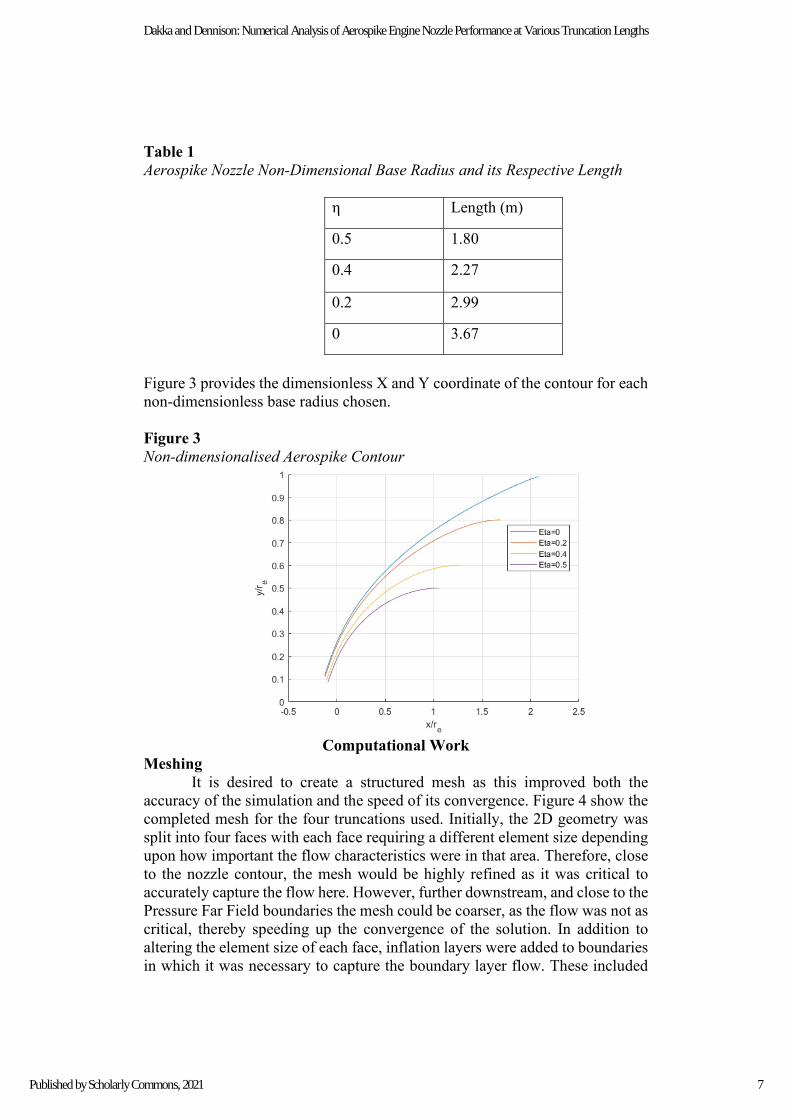
Table 1 Aerospike Nozzle Non-Dimensional Base Radius and its Respective Length

η Length (m)

0.5 1.80

0.4 2.27

0.2 2.99

0 3.67

Figure 3 provides the dimensionless X and Y coordinate of the contour for each non-dimensionless base radius chosen. Figure 3 Non-dimensionalised Aerospike Contour

Computational Work Meshing It is desired to create a structured mesh as this improved both the accuracy of the simulation and the speed of its convergence. Figure 4 show the completed mesh for the four truncations used. Initially, the 2D geometry was split into four faces with each face requiring a different element size depending upon how important the flow characteristics were in that area. Therefore, close to the nozzle contour, the mesh would be highly refined as it was critical to accurately capture the flow here. However, further downstream, and close to the Pressure Far Field boundaries the mesh could be coarser, as the flow was not as critical, thereby speeding up the convergence of the solution. In addition to altering the element size of each face, inflation layers were added to boundaries in which it was necessary to capture the boundary layer flow. These included

7



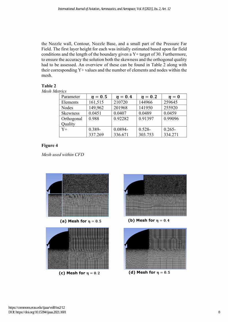
the Nozzle wall, Contour, Nozzle Base, and a small part of the Pressure Far Field. The first layer height for each was initially estimated based upon far field conditions and the length of the boundary given a Y+ target of 30. Furthermore, to ensure the accuracy the solution both the skewness and the orthogonal quality had to be assessed. An overview of these can be found in Table 2 along with their corresponding Y+ values and the number of elements and nodes within the mesh. Table 2 Mesh Metrics

Parameter 𝜼𝜼 = 𝟎𝟎.𝟓𝟓 𝜼𝜼 = 𝟎𝟎.𝟒𝟒 𝜼𝜼 = 𝟎𝟎.𝟐𝟐 𝜼𝜼 = 𝟎𝟎 Elements 161,515 210720 144966 259645 Nodes 149,962 201968 141950 255920 Skewness 0.0451 0.0407 0.0489 0.0459 Orthogonal Quality

0.988 0.92282 0.91397 0.99096

Y+ 0.389-337.269

0.0894-336.671

0.528-303.753

0.265-334.271

Figure 4

Mesh used within CFD

(a) Mesh for 𝛈𝛈 = 𝟎𝟎.𝟓𝟓 (b) Mesh for 𝛈𝛈 = 𝟎𝟎.𝟒𝟒

(c) Mesh for 𝛈𝛈 = 𝟎𝟎.𝟐𝟐 (d) Mesh for 𝛈𝛈 = 𝟎𝟎.𝟓𝟓

8



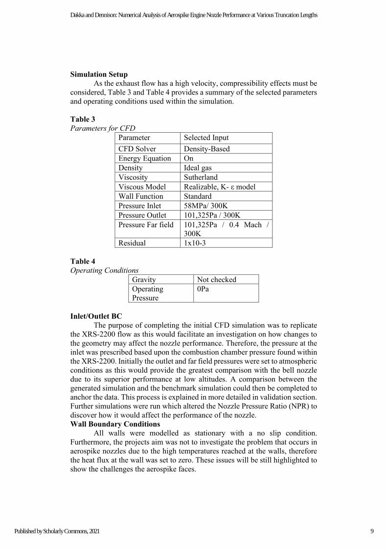
Simulation Setup As the exhaust flow has a high velocity, compressibility effects must be considered, Table 3 and Table 4 provides a summary of the selected parameters and operating conditions used within the simulation. Table 3 Parameters for CFD

Parameter Selected Input CFD Solver Density-Based Energy Equation On Density Ideal gas Viscosity Sutherland Viscous Model Realizable, K- ε model Wall Function Standard Pressure Inlet 58MPa/ 300K Pressure Outlet 101,325Pa / 300K Pressure Far field 101,325Pa / 0.4 Mach /

300K Residual 1x10-3

Table 4 Operating Conditions

Gravity Not checked Operating Pressure

0Pa

Inlet/Outlet BC The purpose of completing the initial CFD simulation was to replicate the XRS-2200 flow as this would facilitate an investigation on how changes to the geometry may affect the nozzle performance. Therefore, the pressure at the inlet was prescribed based upon the combustion chamber pressure found within the XRS-2200. Initially the outlet and far field pressures were set to atmospheric conditions as this would provide the greatest comparison with the bell nozzle due to its superior performance at low altitudes. A comparison between the generated simulation and the benchmark simulation could then be completed to anchor the data. This process is explained in more detailed in validation section. Further simulations were run which altered the Nozzle Pressure Ratio (NPR) to discover how it would affect the performance of the nozzle. Wall Boundary Conditions All walls were modelled as stationary with a no slip condition. Furthermore, the projects aim was not to investigate the problem that occurs in aerospike nozzles due to the high temperatures reached at the walls, therefore the heat flux at the wall was set to zero. These issues will be still highlighted to show the challenges the aerospike faces.

9



Turbulence Modelling Further changes were made to the viscous model, utilising a Realizable, K- ε model, with a standard wall function. The Realizable variation of the viscous model was chosen due to its inclusions of a new transport equations for the dissipation rate, ε. As a result, the turbulence model shows improved performance for many different flow types, namely round jets, and recirculation (Fernández-Yáñez et al., 2017). The standard wall function was chosen due to the calculated Y+ values of the mesh, these were found to be approximately 300 at the boundaries where it was important to capture the flow, thus confirming that the logarithmic law can be used at the wall. Materials In addition to the density-based solver having been chosen, it is necessary to model the density of the fluid as an ideal gas due to compressibility effects. The viscosity was additionally altered from a constant, instead using Sutherlands Law which uses temperature to calculate the fluids viscosity at each node given by:

𝑆𝑆 = 𝐶𝐶1𝑇𝑇32

𝑇𝑇+𝑆𝑆 (20)

Solution Methods The spatial discretisation schemes used can be found within Table 5. Table 5 Solutions Methods

Gradient Least Squares Cell Based

Flow Second Order Upwind

Turbulent Kinetic Energy

QUICK

Turbulent Dissipation Rate

QUICK

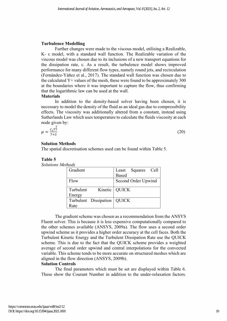
The gradient scheme was chosen as a recommendation from the ANSYS Fluent solver. This is because it is less expensive computationally compared to the other schemes available (ANSYS, 2009a). The flow uses a second order upwind scheme as it provides a higher order accuracy at the cell faces. Both the Turbulent Kinetic Energy and the Turbulent Dissipation Rate use the QUICK scheme. This is due to the fact that the QUICK scheme provides a weighted average of second order upwind and central interpolations for the convected variable. This scheme tends to be more accurate on structured meshes which are aligned in the flow direction (ANSYS, 2009b). Solution Controls The final parameters which must be set are displayed within Table 6. These show the Courant Number in addition to the under-relaxation factors.

10



Both were used to help the solution to converge. Included within Table 6 is the initialisation method chosen. Table 6 Solution Controls

Methodology To demonstrate the benefits of the aerospike engine when compared to a bell nozzle two different conditions were simulated. Initially, the simulation was set up to replicate that of the XRS-2200, to validate the CFD simulation, which was found to be operating close to its optimum. The thrust could therefore be calculated from equation (3) which in turn be used to calculate the nozzle thrust efficiency. This was a necessary step within the project as it enabled the results gathered from the simulation to be compared to previous papers investigating the nozzle thrust efficiency of bell nozzles. One such paper investigated the performance of both an aerospike and bell nozzle experimentally (Wang et al., 2009) . To test the efficiency of the nozzles at different altitudes the variable NPR was introduced. Simply, this is 𝑃𝑃𝑐𝑐/𝑃𝑃𝑎𝑎 and indicates the altitude at which the engine is operating at. By introducing this variable into the investigation, it is possible to compare the performance of the engine at specified NPRS, against that of the experimental data collected. Initially, the simulation was largely constrained to validate the CFD, therefore, the NPR was found to be approximately 58 due to the combustion pressure equalling 58atm and the ambient pressure set to sea-level. Once the validation step had been completed, the NPR was altered. The second condition chosen for further investigation was when the exhaust flow would be over-expanded. To achieve this, the inlet pressure was lowered to 15atm, thereby providing an NPR of 15. Both NPRs were investigated at all four truncations to provide an in-depth investigation on how these factors affect the performance of the engine. Validation To produce a valid simulation, the data is first anchored to Johnson’s paper as this will ensure the accuracy of the simulation and enable the progression of the project (Johnson, 2019). It provides a benchmark simulation

Courant Number 1

Turbulent Kinetic Energy

0.6

Turbulent Dissipation Rate

0.6

Turbulent Viscosity

0.7

Initialisation Hybrid Initialisation

11



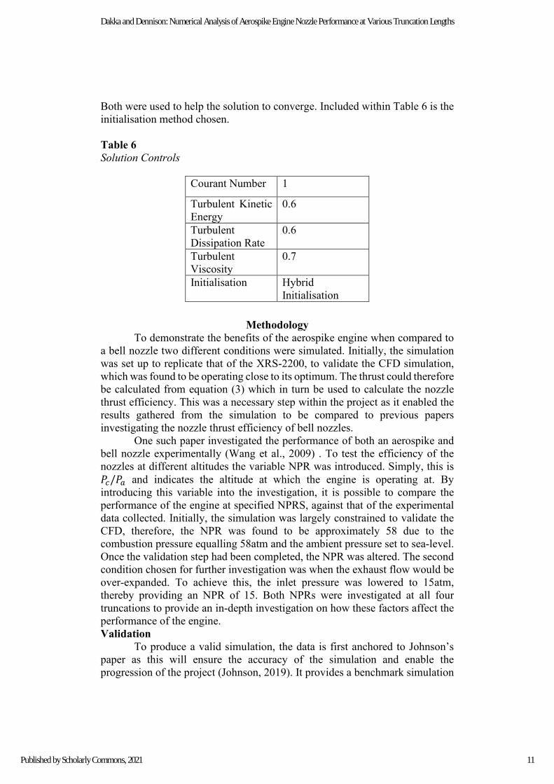
to compare different designs and analyse any performance changes that may occur. Both the flow characteristics and the Mach number along the contour could be analysed to anchor the data and therefore provide confidence with future comparison. Figure 5 shows a velocity vector plot of the nozzle geometry, more like that of the XRS-2200. Within this plot the defining flow characteristics of an aerospike nozzle can be found, namely the re-circulation zone next to the base, the inner shear layer, stagnation point and the envelope shock. These flow characteristics can additionally be found within the paper used to validate the CFD results. Figure 2 Annotated Velocity Vector of Generated Aerospike Nozzle Furthermore, the Mach number along the contour can be examined to further validate the simulation produced. The Mach number varies between 1.8 and 2.92 along the contour. In comparison the benchmark simulation has a Mach number which varies between 1.5 and 3.34 along its contour. This difference amounts to a 20% increase from the minimum benchmark value and a 12.6% decrease from the maximum benchmark value. The Mach contours in combination with the correct flow characteristic being present provide greater confidence to continue with the project now that the data has been anchored.

Results & Discussion Once the data had been anchored to the previously published paper it was possible to vary both the truncation of the nozzle and the conditions it operated at. This would enable a comparison against the existing data which has already been verified to demonstrate any performance gains or reductions which may occur because of the geometry change. It is possible to analyse the results from the CFD simulation qualitatively in addition to the quantitively, these processes will be shown within the next two sections. Qualitative Study of the Results Figure 6 presents the Mach contour for the replicated XRS-2200 geometry, when 𝜂𝜂 = 0.5. As the fluid exits the throat of the thruster it accelerates, exceeding Mach 1. This is the main purpose of the aerospike nozzle

Re-circulation zone

Inner shear layer Stagnation point

Envelope shock

12



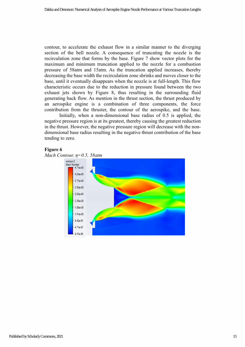
contour, to accelerate the exhaust flow in a similar manner to the diverging section of the bell nozzle. A consequence of truncating the nozzle is the recirculation zone that forms by the base. Figure 7 show vector plots for the maximum and minimum truncation applied to the nozzle for a combustion pressure of 58atm and 15atm. As the truncation applied increases, thereby decreasing the base width the recirculation zone shrinks and moves closer to the base, until it eventually disappears when the nozzle is at full-length. This flow characteristic occurs due to the reduction in pressure found between the two exhaust jets shown by Figure 8, thus resulting in the surrounding fluid generating back flow. As mention in the thrust section, the thrust produced by an aerospike engine is a combination of three components, the force contribution from the thruster, the contour of the aerospike, and the base. Initially, when a non-dimensional base radius of 0.5 is applied, the negative pressure region is at its greatest, thereby causing the greatest reduction in the thrust. However, the negative pressure region will decrease with the non-dimensional base radius resulting in the negative thrust contribution of the base tending to zero. Figure 6 Mach Contour, η=0.5, 58atm

13



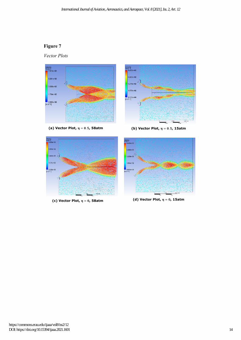
Figure 7

Vector Plots

(a) Vector Plot, 𝛈𝛈 = 𝟎𝟎.𝟓𝟓, 58atm (b) Vector Plot, 𝛈𝛈 = 𝟎𝟎.𝟓𝟓, 15atm

(c) Vector Plot, 𝛈𝛈 = 𝟎𝟎, 58atm (d) Vector Plot, 𝛈𝛈 = 𝟎𝟎, 15atm

14



Figure 8 Pressure Contours

(a) Pressure Contour, 𝛈𝛈 = 𝟎𝟎.𝟓𝟓, 58atm (b) Pressure contour, 𝛈𝛈 = 𝟎𝟎.𝟓𝟓, 15atm

(c) Pressure Contour, 𝛈𝛈 = 𝟎𝟎.𝟒𝟒, 58atm (d) Pressure contour, 𝛈𝛈 = 𝟎𝟎.𝟒𝟒, 15atm

(e) Pressure Contour, 𝛈𝛈 = 𝟎𝟎.𝟐𝟐 58atm (f) Pressure contour, 𝛈𝛈 = 𝟎𝟎.𝟐𝟐, 15atm

15



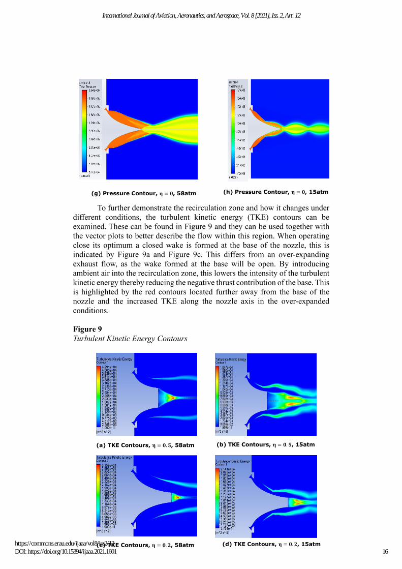
To further demonstrate the recirculation zone and how it changes under different conditions, the turbulent kinetic energy (TKE) contours can be examined. These can be found in Figure 9 and they can be used together with the vector plots to better describe the flow within this region. When operating close its optimum a closed wake is formed at the base of the nozzle, this is indicated by Figure 9a and Figure 9c. This differs from an over-expanding exhaust flow, as the wake formed at the base will be open. By introducing ambient air into the recirculation zone, this lowers the intensity of the turbulent kinetic energy thereby reducing the negative thrust contribution of the base. This is highlighted by the red contours located further away from the base of the nozzle and the increased TKE along the nozzle axis in the over-expanded conditions. Figure 9 Turbulent Kinetic Energy Contours

(a) TKE Contours, 𝛈𝛈 = 𝟎𝟎.𝟓𝟓, 58atm (b) TKE Contours, 𝛈𝛈 = 𝟎𝟎.𝟓𝟓, 15atm

(c) TKE Contours, 𝛈𝛈 = 𝟎𝟎.𝟐𝟐, 58atm (d) TKE Contours, 𝛈𝛈 = 𝟎𝟎.𝟐𝟐, 15atm

(g) Pressure Contour, 𝛈𝛈 = 𝟎𝟎, 58atm (h) Pressure Contour, 𝛈𝛈 = 𝟎𝟎, 15atm

16



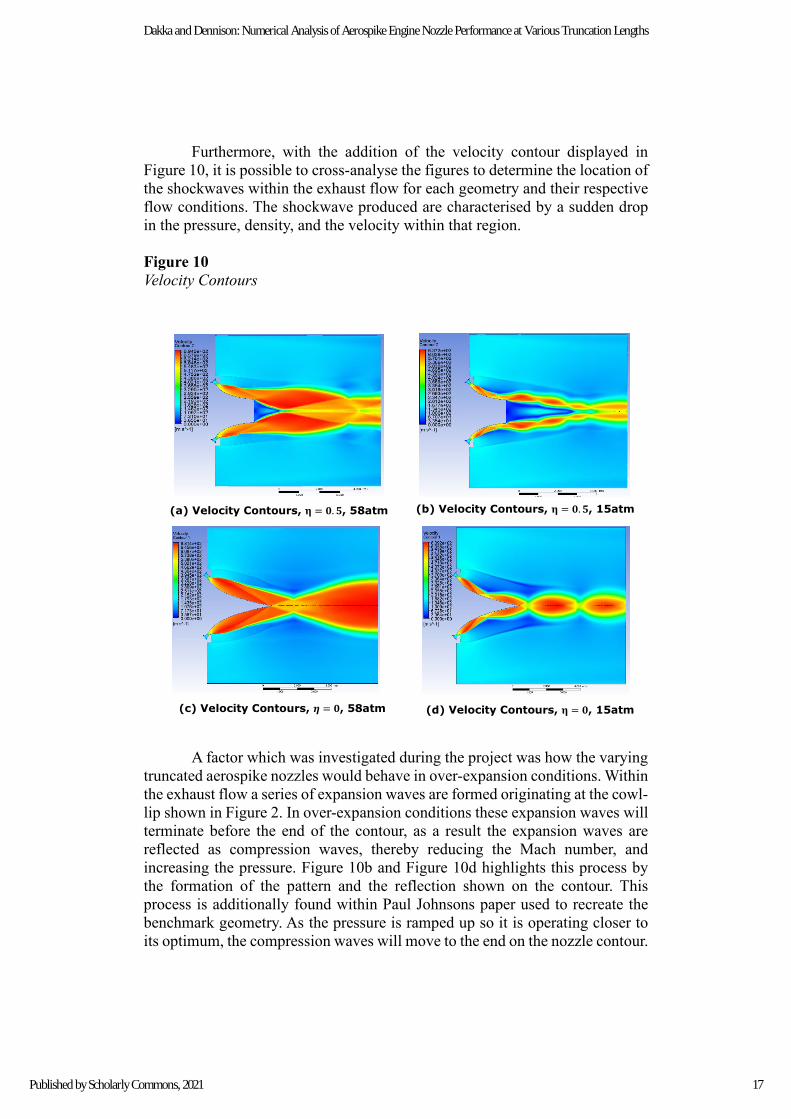
Furthermore, with the addition of the velocity contour displayed in Figure 10, it is possible to cross-analyse the figures to determine the location of the shockwaves within the exhaust flow for each geometry and their respective flow conditions. The shockwave produced are characterised by a sudden drop in the pressure, density, and the velocity within that region. Figure 10 Velocity Contours A factor which was investigated during the project was how the varying truncated aerospike nozzles would behave in over-expansion conditions. Within the exhaust flow a series of expansion waves are formed originating at the cowl-lip shown in Figure 2. In over-expansion conditions these expansion waves will terminate before the end of the contour, as a result the expansion waves are reflected as compression waves, thereby reducing the Mach number, and increasing the pressure. Figure 10b and Figure 10d highlights this process by the formation of the pattern and the reflection shown on the contour. This process is additionally found within Paul Johnsons paper used to recreate the benchmark geometry. As the pressure is ramped up so it is operating closer to its optimum, the compression waves will move to the end on the nozzle contour.

(a) Velocity Contours, 𝛈𝛈 = 𝟎𝟎.𝟓𝟓, 58atm

(c) Velocity Contours, 𝜼𝜼 = 𝟎𝟎, 58atm

(b) Velocity Contours, 𝛈𝛈 = 𝟎𝟎.𝟓𝟓, 15atm

(d) Velocity Contours, 𝛈𝛈 = 𝟎𝟎, 15atm

17



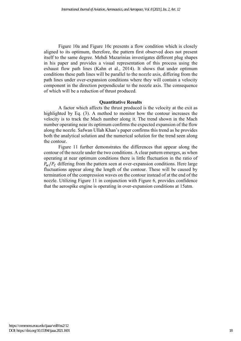
Figure 10a and Figure 10c presents a flow condition which is closely aligned to its optimum, therefore, the pattern first observed does not present itself to the same degree. Mehdi Mazarinias investigates different plug shapes in his paper and provides a visual representation of this process using the exhaust flow path lines (Kahn et al., 2014). It shows that under optimum conditions these path lines will be parallel to the nozzle axis, differing from the path lines under over-expansion conditions where they will contain a velocity component in the direction perpendicular to the nozzle axis. The consequence of which will be a reduction of thrust produced.

Quantitative Results A factor which affects the thrust produced is the velocity at the exit as highlighted by Eq. (3). A method to monitor how the contour increases the velocity is to track the Mach number along it. The trend shown in the Mach number operating near its optimum confirms the expected expansion of the flow along the nozzle. Safwan Ullah Khan’s paper confirms this trend as he provides both the analytical solution and the numerical solution for the trend seen along the contour. Figure 11 further demonstrates the differences that appear along the contour of the nozzle under the two conditions. A clear pattern emerges, as when operating at near optimum conditions there is little fluctuation in the ratio of 𝑃𝑃𝑤𝑤/𝑃𝑃𝐶𝐶 differing from the pattern seen at over-expansion conditions. Here large fluctuations appear along the length of the contour. These will be caused by termination of the compression waves on the contour instead of at the end of the nozzle. Utilizing Figure 11 in conjunction with Figure 6, provides confidence that the aerospike engine is operating in over-expansion conditions at 15atm.

18



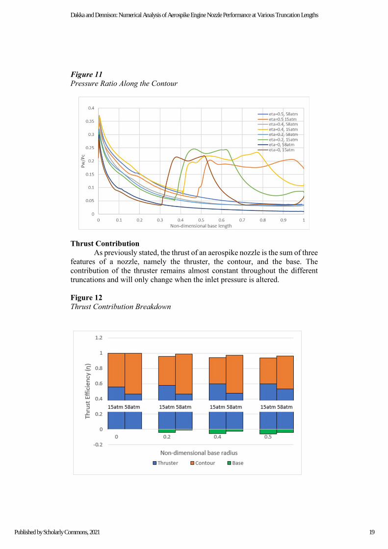
Figure 11 Pressure Ratio Along the Contour

Thrust Contribution As previously stated, the thrust of an aerospike nozzle is the sum of three features of a nozzle, namely the thruster, the contour, and the base. The contribution of the thruster remains almost constant throughout the different truncations and will only change when the inlet pressure is altered. Figure 12 Thrust Contribution Breakdown

19



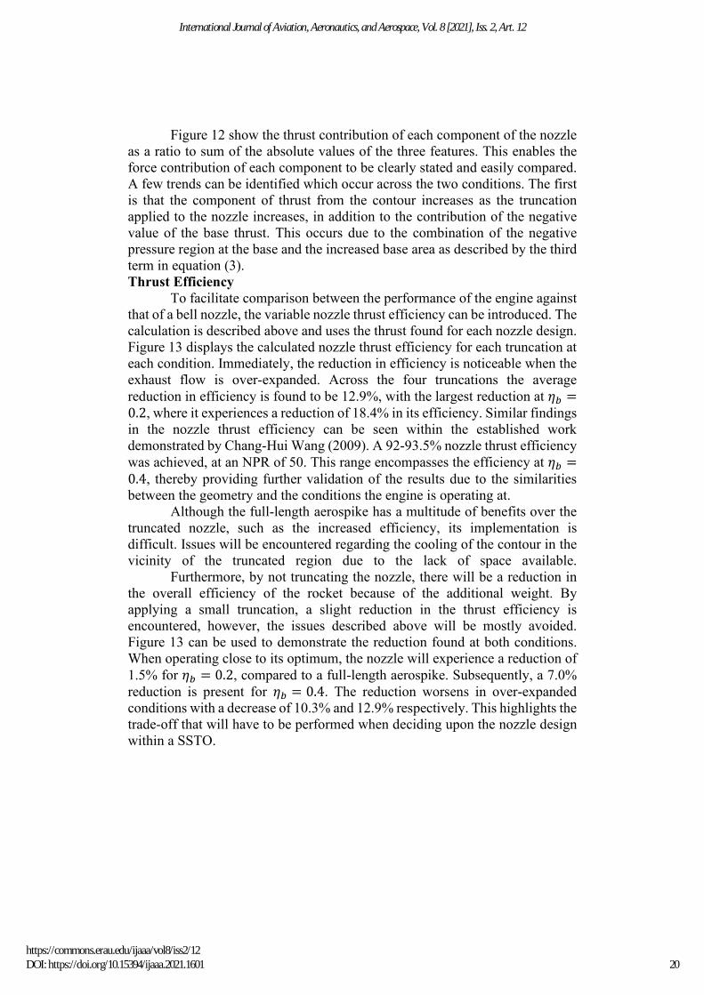
Figure 12 show the thrust contribution of each component of the nozzle as a ratio to sum of the absolute values of the three features. This enables the force contribution of each component to be clearly stated and easily compared. A few trends can be identified which occur across the two conditions. The first is that the component of thrust from the contour increases as the truncation applied to the nozzle increases, in addition to the contribution of the negative value of the base thrust. This occurs due to the combination of the negative pressure region at the base and the increased base area as described by the third term in equation (3). Thrust Efficiency To facilitate comparison between the performance of the engine against that of a bell nozzle, the variable nozzle thrust efficiency can be introduced. The calculation is described above and uses the thrust found for each nozzle design. Figure 13 displays the calculated nozzle thrust efficiency for each truncation at each condition. Immediately, the reduction in efficiency is noticeable when the exhaust flow is over-expanded. Across the four truncations the average reduction in efficiency is found to be 12.9%, with the largest reduction at 𝜂𝜂𝑎𝑎 =0.2, where it experiences a reduction of 18.4% in its efficiency. Similar findings in the nozzle thrust efficiency can be seen within the established work demonstrated by Chang-Hui Wang (2009). A 92-93.5% nozzle thrust efficiency was achieved, at an NPR of 50. This range encompasses the efficiency at 𝜂𝜂𝑎𝑎 =0.4, thereby providing further validation of the results due to the similarities between the geometry and the conditions the engine is operating at. Although the full-length aerospike has a multitude of benefits over the truncated nozzle, such as the increased efficiency, its implementation is difficult. Issues will be encountered regarding the cooling of the contour in the vicinity of the truncated region due to the lack of space available. Furthermore, by not truncating the nozzle, there will be a reduction in the overall efficiency of the rocket because of the additional weight. By applying a small truncation, a slight reduction in the thrust efficiency is encountered, however, the issues described above will be mostly avoided. Figure 13 can be used to demonstrate the reduction found at both conditions. When operating close to its optimum, the nozzle will experience a reduction of 1.5% for 𝜂𝜂𝑎𝑎 = 0.2, compared to a full-length aerospike. Subsequently, a 7.0% reduction is present for 𝜂𝜂𝑎𝑎 = 0.4. The reduction worsens in over-expanded conditions with a decrease of 10.3% and 12.9% respectively. This highlights the trade-off that will have to be performed when deciding upon the nozzle design within a SSTO.

20



Figure 13 Thrust Efficiency

The results gathered from the CFD simulation can be compared to the expected nozzle thrust efficiency for both the aerospike nozzle and the bell nozzle. The results for the experimental data were taken from the paper by Chang-Hui Wang and are displayed in Figure 14. When the engine is operating close to its optimum, at an NPR of 58, each truncation demonstrates an increased nozzle thrust efficiency over the bell nozzle. This occurs due to the rapid reduction of the nozzle thrust efficiency when operating in over-expanded conditions for the bell nozzle. The rate of this decrease is greater than that of the aerospike nozzle which still shows a reduction, but not to the same extent as the bell nozzle. The over-expanded conditions were specified to demonstrate the effects over-expansion has on the aerospike nozzle. Although, this engine design would not be operating at an NPR within this region, and instead would be operating at NPRs greater than 58 due to 58 being set to sea-level, it still has a greater performance. Above an NPR of 58, it is expected that the nozzle thrust efficiencies will closely follow the experimental aerospike nozzle. The beginning of this trend is noticeable within the figure as they show a great increase in the efficiency by a relatively small increase of NPR for all truncations.

00.10.20.30.40.50.60.70.80.9

1

0 0.2 0.4 0.5

Thru

st E

ffici

ency

(η)

Aerospike Truncation58atm 15atm

21



Figure 14 Comparison of Nozzle Thrust Efficiency

Conclusions The flow characteristics and various performance indicators have been analysed to determine the effect of truncating the nozzle at near optimum and over-expansion conditions. The vector plots in addition to the velocity contours clearly demonstrate the effect the varying conditions have on the exhaust flow, as the recirculating flow region will become larger in over-expansion conditions and producing an open wake. In comparison a closed wake is formed at near optimum conditions. As a result, the negative thrust contribution of the base increases with respect to optimum conditions. This effect is accentuated when the pressure at the inlet is increased. The results further indicate that as the truncation applied to the nozzle increases, the nozzle thrust efficiency decreases, with it performing worse in over-expansion conditions due to the compression waves terminating earlier on the contour. As a full spike is impractical due to the additional weight and cooling issues stated, 𝜂𝜂𝑎𝑎 = 0.2, 0.4 provide relatively small reduction in efficiency at both conditions, particularly 𝜂𝜂𝑎𝑎 = 0.2. However, the issues described for the full spike will still be present for these designs, but not to the same extent. At near optimum conditions, all aerospike nozzles demonstrate a performance gain over the bell nozzle. This is due to the rapid decline in the bell nozzles efficiency at low altitudes, differing from the aerospike nozzle. This is highlighted by a greater performance of the aerospike nozzle at a lower NPR.

22



References Angelino, G. (1964). Approximate method for plug nozzle design. AIAA,

2(10), 1834–1835. doi:10.2514/3.2682 ANSYS. (2009a). Evaluation of gradients and derivatives.

https://www.afs.enea.it/project/neptunius/docs/fluent/html/th/node368.htm

ANSYS. (2009b). Spatial discretization. https://www.afs.enea.it/project/ neptunius/ docs/fluent/html/th/node366.htm

Bani, A. A. (2016). Design and analysis of an axisymmetric aerospike supersonic micro-nozzle for a refridgerant-based cold-gas propulsion system opulsion system for small satellites. https://www.researchgate.net/publication/323161530_Design_of_axisymmetric_aerospike_nozzle_based_on_modified_MOC

Bergin, C. (2006). X-33/VentureStar – What really happened. NASA Space Flight. https://www.nasaspaceflight.com/2006/01/x-33venturestar-what-really-happened/

Boeing. (1997). XRS-2200 linear aerospike engine. https://engineering.purdue.edu/~propulsi/propulsion/rockets/liquids/xrs2200.html

Bravo, L., & Ihme, M. (2017). Breakthroughs in engine propulsion research with high-performance computing: DSIAC Journal, 4(4), 1–39, 2017.

Fernández-Yáñez, F., Armas, O., Gómez, A., & Gil, A. (2017). Developing computational fluid dynamics (CFD) models to evaluate available energy in exhaust systems of diesel light-duty vehicles. Applies Science, 7(6), 1-20. doi:10.3390/app7060590

Johnson, P. (2019). CFD analysis of a linear aerospike engine with film - cooling. https://www.sjsu.edu/ae/docs/project-thesis/Paul.Johnson-Su19.pdf

Khan, S. U., Khan, A. A., & Munir, A. (2014). Design and analysis approach for linear aerospike nozzle. COMSATS Sci. Vis., 20, 25–38.

Nazarinia, M., Naghib-Lahouti, A., & Tolouei, E. (2005). Design and numerical analysis of aerospike nozzles with different plug shapes to compare their performance with a conventional nozzle. The Eleventh Australian International Aerospace Congress (AIAC-11), Melbourne Convention Centre, Melbourne, Australia, 13-17 March 2005.

Rao, G. V. R. (1958). Exhaust nozzle contour for optimum thrust. Journal of Jet Propulsion, 28(6), 377–382, Jun. 1958, doi:10.2514/8.7324

Rao, G. V. R. (1961). Spike nozzle contour for optimum thrust. Planetary and Space Science, 4, 92–101. doi:10.1016/0032-0633(61)90125-8

Rocketdyne. (1972). Linear test bed final report. https://alternatewars.com/ BBOW/Space_Engines/LinearTestBed_Vol2.pdf

Wang, C.-H, Liu, Y., & Qin, L.-Z. (2009). Aerospike nozzle contour design and its performance validation. Acta Astronaut, 64, (11–12), 1264–1275. doi:10.1016/j.actaastro.2008.01.045

23



numerical analysis of aerospike engine nozzle performance

Documents