del servizio studi - banca d'italia · temi di discussione del servizio studi new eurocoin:...
TRANSCRIPT

Temi di discussionedel Servizio Studi
New Eurocoin: Tracking economic growth in real time
Number 631 - June 2007
by Filippo Altissimo, Riccardo Cristadoro, Mario Forni, Marco Lippi and Giovanni Veronese

The purpose of the Temi di discussione series is to promote the circulation of working papers prepared within the Bank of Italy or presented in Bank seminars by outside economists with the aim of stimulating comments and suggestions.
The views expressed in the articles are those of the authors and do not involve the responsibility of the Bank.
Editorial Board: DOMENICO J. MARCHETTI, MARCELLO BOFONDI, MICHELE CAIVANO, STEFANO IEZZI, ANDREA LAMORGESE, FRANCESCA LOTTI, MARCELLO PERICOLI, MASSIMO SBRACIA, ALESSANDRO SECCHI, PIETRO TOMMASINO.Editorial Assistants: ROBERTO MARANO, ALESSANDRA PICCININI.

NEW EUROCOIN: TRACKING ECONOMIC GROWTH IN REAL TIME*
by Filippo Altissimo**, Riccardo Cristadoro***, Mario Forni****, Marco Lippi*****, and Giovanni Veronese***
Abstract
This paper presents ideas and methods underlying the construction of an indicator that tracks euro-area GDP growth but, unlike GDP growth, (i) is updated monthly and almost in real time, and (ii) is free from short-run dynamics. Removal of short-run dynamics from a time series to isolate the medium to long-run component can be obtained by a band-pass filter. However, it is well known that band-pass filters, being two-sided, perform very poorly at the end of the sample. New Eurocoin is an estimator of the medium to long-run component of GDP that only uses contemporaneous values of a large panel of macroeconomic time series, so that no end-of-sample deterioration occurs. Moreover, as our dataset is monthly, New Eurocoin can be updated each month and with a very short delay. Our method is based on generalized principal components that are designed to use leading variables in the dataset as proxies for future values of GDP growth. As the medium to long-run component of GDP is observable, although with delay, the performance of New Eurocoin at the end of the sample can be measured.
JEL Classification: C51; E32; O30. Keywords: coincident indicator, band-pass filter, large-dataset factor models, generalized principal components.
* We gratefully acknowledge encouragement and support from the Bank of Italy and the Centre for Economic Policy Research. We thank Marc Hallin for his suggestions at an early stage of the project, Antonio Bassanetti for his ideas and unique expertise in the realization of the currently published version of Eurocoin indicator and, in particular, Lucrezia Reichlin who started and promoted the Eurocoin project. We also thank those who gave suggestions and comments over the years, among them: Andreas Fisher, Domenico Giannone, James Stock, Mark Watson and two anonymous referees at the Bank of Italy. The views expressed here do not necessarily reflect those of the Bank of Italy, the European Central Bank, or any other institutions with which the authors are affiliated. Correspondence: [email protected] ** Brevan Howard Asset Management. *** Bank of Italy, Economic Research Department. **** Università di Modena e Reggio Emilia and CEPR. *****Università di Roma ‘La Sapienza’.

Contents
1. Introduction........................................................................................................................... 5
2. Preliminary observations ...................................................................................................... 7
3. The MLRG and its interpretation ....................................................................................... 10
4. Estimation I: Projecting the MLRG on monthly regressors ............................................... 13
5. Estimation II: Constructing the regressors ......................................................................... 16
6. Results ................................................................................................................................. 21
6.1 New Eurocoin indicator ........................................................................................... 21
6.2 The real-time performance....................................................................................... 22
6.3 The behavior around turning points ......................................................................... 25
6.4 The forecasting properties of the indicator .............................................................. 27
7. Summary and conclusion .................................................................................................... 29
Appendix A: Technical details ................................................................................................ 30
A.1 Computing c*t ........................................................................................................30
A.2 Estimating Σw and Σcw............................................................................................ 32
A.3 Estimating ΣФ, Σχ and Σξ........................................................................................ 32
Appendix B: Dataset and treatment......................................................................................... 34
References ............................................................................................................................... 35
Data description....................................................................................................................... 38

1 Introduction
This paper presents a method to estimate in real time the current state of the economy.
The method is applied to the euro area, the geographical focus being motivated by the
creation of the European Monetary Union and the implementation of a common monetary
policy. The resulting indicator, New Eurocoin (NE henceforth), is intended to replace the
Eurocoin indicator proposed by Altissimo et al. (2001) and published monthly by the
Centre for Economic Policy Research (see the website www.cepr.org).
The main objective of our indicator is to make an assessment of economic activity
that is (a) comprehensive and non-subjective, (b) timely and (c) free from short-run
fluctuations. None of the available macroeconomic series provides a measure of the state
of the economy that fulfills all such criteria. GDP, the most comprehensive indicator
of real activity, fails to meet (b) and (c). Regarding timeliness, GDP is only available
quarterly and with a long delay. For instance, the preliminary estimate of euro area GDP
for the first quarter of the year becomes available only in May. Moreover, GDP is affected
by a sizeable short-run component so that, for example, the beginning of a medium-run
upswing cannot be distinguished from a transitory upward movement within a basically
negative path.
NE is a real-time estimate of GDP growth, cleaned of short-run oscillations. More
precisely,
(i) We focus on the growth rate of GDP and define the medium to long-run growth,
henceforth denoted by MLRG, as the component of the GDP growth rate obtained by
removing the fluctuations of a period shorter than or equal to one year. This medium to
long-run component of the GDP growth rate will be our target.
(ii) NE is a monthly and timely estimate of the MLRG for the euro area: by the 25th of
each month we are able to produce a reliable estimate for the current month.
Based on the spectral representation of a stationary process, MLRG is defined as
including only the oscillations of period longer than one year, and is therefore a “smooth-
ing” of GDP growth. As is well known, such a result can be achieved by applying to
GDP growth a band-pass filter that removes high-frequency waves. However, the ideal
band-pass filter is an infinite, centred, moving average. The effect of truncation is not
uniform over finite samples, with endpoints badly estimated and severely revised as new
data become available (see e.g. Baxter and King, 1999; Christiano and Fitzgerald, 2003).
A substantial mitigation of this conflict between timeliness and removal of the short-
5

run fluctuations is the main contribution of the present paper. We obtain a good smooth-
ing by exploiting cross-sectional current information from a large dataset. The intuition is
that the dataset contains variables that are leading with respect to current GDP. There-
fore the information contained in the future of GDP, which is unavailable, can be partially
recovered by projecting the MLRG onto a suitable set of linear combinations of current
values of these variables.
Constructing such linear combinations is the crucial step of our procedure. We start
with a large dataset, containing variables that are closely related to the MLRG. To es-
timate our unobserved component we could select a small number of them. However,
the macroeconomic series used as regressors would necessarily contain a good deal of id-
iosyncratic (i.e. specific to variable, country, sector, etc.) and short-run noise, which is
harmful to the estimation of our indicator. The central idea is that instead of selecting
a few macroeconomic variables we can employ a small number of linear combinations of
the series in the dataset, in such a way as to remove both variable-specific and short-run
sources of fluctuation, while retaining cyclical and long-run movements. To do so we
use a particular kind of principal components, which are specifically designed to extract
from the dataset the common, medium to long-run information. More precisely, we take
the linear combinations of the observable series whose fraction of common, medium to
long-run variance is maximal.
Common medium to long-run variance is estimated using the Generalized Dynamic
Factor Model (GDFM) proposed by Forni, Hallin, Lippi and Reichlin (2000) and Forni and
Lippi (2001). The use of factor models is not new in the literature on coincident indicators,
an important reference being Stock and Watson (1989), where the “cycle” is defined as
the unique common factor, loaded contemporaneously by a few coincident variables. By
contrast, our model is designed to handle a large number of variables affected by more
than one common source of variation. Moreover, the factors are loaded with quite general
impulse-response functions, so as to represent leading, coincident and lagging series (for
models with these features, see also Stock and Watson 2002a, 2002b).
Let us point out that NE is not an estimate of a latent variable, being different in this
respect from the coincident indicators constructed e.g. in Stock and Watson (1989), those
routinely produced by OECD and other international organizations, and the currently
published Eurocoin. Rather, NE is defined as a real time estimate of the medium to long-
run component of GDP growth, and the latter is observable, although with a long delay.
As a consequence, the performance of our indicator can be measured. More precisely, the
6

value of the target, which is not available at the end-of-sample time T (the band-pass
filter performing very poorly), becomes available with good accuracy at time T + h, for a
suitable h. Therefore our indicator, produced at time T , can be compared with the target
at T produced at time T + h.1 We believe that these features, an observable target and
a measure of performance, represent a substantial improvement over the abovementioned
literature.
Our dataset includes monthly series of production prices, wages, share prices, money,
unemployment rates, job vacancies, interest rates, exchange rates, industrial production,
orders, retail sales, imports, exports, and consumer and business surveys for the euro
area countries and the euro area as a whole (see Appendix B for details). The dataset
has been organized taking into account the calendar of data releases that is typical in
real situations, with the aim of reproducing the staggered flow of information available
through time to policy-makers and market forecasters. This lack of synchronism, though
little considered in the literature, is crucial for assessing realistically the performance of
alternative real-time indicators.2
The paper is organized as follows. Section 2 collects some preliminary observations.
Section 3 defines our target, i.e. the medium to long-run component of GDP, and discusses
its interpretation. Sections 4 and 5 describe and motivate our estimation procedure.
Section 6 shows the New Eurocoin indicator, analyzes its real-time performance and
compares it with a few alternative indicators. Section 7 concludes. Technical details
are presented in Appendix A. Appendix B describes the dataset and data treatment.
2 Preliminary observations
To gauge the current state of the economy, given the delay with which GDP is released,
market analysts and forecasters resort to more timely and high frequency information and
on this basis obtain early estimates of GDP. However, two problems immediately arise:
(i) looking at the typical release calendar for the euro area, one can see that timeliness
varies greatly even among monthly statistics (end-of-sample unbalance); (ii) since GDP
is quarterly we have to handle simultaneously monthly and quarterly data.
Here we combine the comprehensive and non-subjective information provided by GDP
1Recent papers providing direct estimates of current activity, as opposed to estimates of latent vari-ables, are Mitchell et al. (2004) and Evans (2005).
2Important exceptions are Bernanke and Boivin (2003) and Giannone et. al. (2002).
7

with the early information provided by surveys and other monthly series to obtain a
reliable and timely picture of current economic activity.
Table 1: The calendar of some macroeconomic series
Time DEC. 04 GEN. 05 FEB. 05 MAR. 05 APR. 05 MAY 05 JUN. 05
Release date
Delay
Q3 - 2004 Q3 - 2004 Q4 - 2004 Q4 - 2004 Q4 - 2004 Q1-2005 Q1-2005 45-90 days
Industrial production Oct. 04 Nov. 04 Dec. 04 Jan. 05 Feb. 05 Mar. 05 Apr. 05 45-50 days
Dec. 04 Jan. 05 Feb. 05 Mar. 05 Apr. 05 May. 05 Jun. 05 0-25 days
Retail sales Oct. 04 Nov. 04 Dec. 04 Jan. 05 Feb. 05 Mar. 05 Apr. 05 45-50 days
Financial markets Dec. 04 Jan. 05 Feb. 05 Mar. 05 Apr. 05 May. 05 Jun. 05 0 days
Nov. 04 Dec. 04 Jan. 05 Feb. 05 Mar. 05 Apr. 05 May. 05 15 days
Car registrations Nov. 04 Dec. 04 Jan. 05 Feb. 05 Mar. 05 Apr. 05 May. 05 2-30 days
Industrial orders Oct. 04 Nov. 04 Dec. 04 Jan. 05 Feb. 05 Mar. 05 Apr. 05 50 days
Surveys
CPI
GDP
Real time information sets
As shown in Table 1, Financial Variables and Surveys are the most timely data, while
Industrial Production and other “real variables” are usually available with longer delays.
Towards the end of month T , when we calculate the indicator for the same month T ,
Surveys and Financial Variables are usually observed up to time T (thus with no delay),
Car Registration and Industrial Orders up to T − 1 and Industrial Production indices
up to T − 2 or T − 3. The GDP series is observed quarterly, so that its delay varies
with time. For example, in April only data up to the fourth quarter of the previous
year are available, while during the first half of May the delay is reduced as first-quarter
preliminary estimates are released.
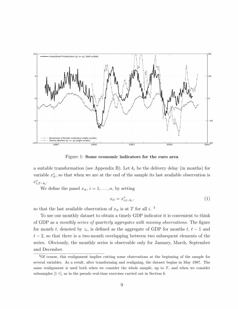
The most timely variables (such as Purchasing Managers Indexes, Consumer Surveys,
Business Climate Indexes, etc.) are usually far from being comprehensive and smooth.
Other standard series, such as Industrial Production and Exports, ignore large portions
of economic activity and are less timely. Furthermore, all of them exhibit heavy short-
run fluctuations and might provide contradictory signals, see Figure 1. As a result, none
of them is fully satisfactory and “there is much diversity and uncertainty about which
indicators are to be used” (Zarnowitz and Ozyildirim, 2002).
We tackle the end-of-sample unbalance in the following way. Let x∗it, i = 1, . . . , n, be
the series after outliers and seasonality have been removed and stationarity achieved by
8
1987 1992 1997 2002 2007−10
−5
0
5
10
−50
−25
0
25
50
Industrial Production (y−o−y), (left scale)
Business Climate Indicator (right scale)Stock Market (y−o−y),(right scale)
Figure 1: Some economic indicators for the euro area
a suitable transformation (see Appendix B). Let ki be the delivery delay (in months) for
variable x∗it, so that when we are at the end of the sample its last available observation is
x∗i,T−ki.
We define the panel xit, i = 1, . . . , n, by setting
xit = x∗i,t−ki, (1)
so that the last available observation of xit is at T for all i. 3
To use our monthly dataset to obtain a timely GDP indicator it is convenient to think
of GDP as a monthly series of quarterly aggregates with missing observations. The figure
for month t, denoted by zt, is defined as the aggregate of GDP for months t, t − 1 and
t − 2, so that there is a two-month overlapping between two subsequent elements of the
series. Obviously, the monthly series is observable only for January, March, September
and December.3Of course, this realignment implies cutting some observations at the beginning of the sample for
several variables. As a result, after transforming and realigning, the dataset begins in May 1987. Thesame realignment is used both when we consider the whole sample, up to T , and when we considersubsamples [1 τ ], as in the pseudo real-time exercises carried out in Section 6.
9

The monthly GDP growth rate is defined as
yt = log zt − log zt−3.
Thus yt is the usual quarter-on-quarter growth rate, except that it is defined for all months.
How to deal with the missing observations in GDP will be discussed in detail in Section
3 and in Appendix A.1.
3 The MLRG and its interpretation
A natural way to define the medium to long-run fluctuations of a time series is by con-
sidering its spectral decomposition. Assuming stationarity, yt can be represented as an
integral of sine and cosine waves with stochastic weights. This is the well-known spectral
representation (see e.g. Brockwell and Davis, 1991, ch. 4). We can distinguish long and
medium waves, say ct, from short waves, say st, by splitting the integral into two parts,
corresponding to complementary frequency intervals, separated by a threshold value. The
choice of the threshold π/6 is quite natural in our context, since it corresponds to a period
of one year: we are not interested in seasonality and other higher frequency waves.
Here we do not delve into the details of the band-pass filter and go directly to the result
(see e.g. Baxter and King, 1999, and Christiano and Fitzgerald, 2003). The medium to
long-run component ct is the following infinite, symmetric, two-sided linear combination
of the GDP growth series:
ct = β(L)yt =∞∑
k=−∞
βkyt−k, βk =
sin(kπ/6)
kπfor k 6= 0
1/6 for k = 0.(2)
The filter β(L) is the low-pass filter which selects waves of frequency smaller than π/6.
Our decomposition is then
yt = ct + st = β(L)yt + [1− β(L)]yt. (3)
Since β(1) = 1, the mean of the GDP growth series, denoted by µ, is retained in ct
while the mean of st is zero. The variance of yt is broken down into the sum of a short-
run variance and a medium to long-run variance, because ct and st are orthogonal. The
medium to long-run component ct is our theoretical target MLRG.
Note that ct is referred to as “medium to long-run growth” not as growth-rate cycle
or “business cycle”. Usually, in the definition of a cycle the oscillations of a period longer
10

than 8 years are also removed. This further refinement, though possible in principle, did
not seem interesting for our purpose (for different definitions of the cycle, see Stock and
Watson, 1999).
Two missing-data problems arise with (2):
(i) Suppose firstly that yt is observed monthly. Still the filter β(L) is infinite, so that
within finite samples we can only get approximations of ct. Among different options we
chose the following
c∗t = β(L)y∗t , where y∗t =
yt if 1 ≤ t ≤ T
µ if t < 1 or t > T ,(4)
µ denoting the estimated mean of yt, i.e. the application of the infinite filter β(L) to the
infinite time series obtained by setting the missing values of yt equal to its mean. This is,
of course, equivalent to a t-dependent asymmetric truncation of β(L).
(ii) However, as we know, yt is not observed monthly. Several options are possible,
including linear interpolation of the missing values or the more sophisticated techniques
introduced in Chow and Lin (1971). However, we should keep in mind that the variable we
are interested in is ct not yt. It turns out that for this purpose the particular interpolation
of the missing values in yt makes no significant difference. This may be easily understood
by taking the spectral point of view. Sensible interpolations of the two data point that
are missing for each quarter only have effects on the short-run behaviour of the series.
Since the short waves are filtered out by β(L), the interpolation technique chosen has a
negligible effect.
The result of linearly interpolating the missing data in yt, augmenting yt with its mean,
and applying the filter β(L), will be denoted by c∗t (T ), or c∗t when no confusion can arise.
In the pseudo real-time exercises presented in Section 6 we will consider subsamples [1 τ ],
with τ < T , and the corresponding series c∗t (τ), whose definition is (4) with τ replacing
T . Due to its asymmetry, the approximation provided by c∗t (T ) is very poor at the end
(and the beginning) of the sample, whereas it is extremely good as soon as t is just twelve
months away from T and 1, almost perfect in the centre of the sample. Further details
on the construction on c∗t are given in Appendix A.1.
We henceforth take c∗t (T ), inside the sample, as our target. Precisely, the performance
of NE will be measured by the distance between the value of NE obtained at t and c∗t (T )
with 13 ≤ t ≤ T − 12.
Figure 2 presents the approximation c∗t (T ) for euro zone GDP for 13 ≤ t ≤ T − 12,
along with quarterly GDP growth, yt, where T is August 2005. We see that c∗t closely
11

1988 1992 1996 2000 2004−1.5
−1
−0.5
0
0.5
1
1.5
2
q−o−q GDP growthMLRG
Figure 2: The (approximate) MLRG, c∗t (T ), and the quarter-on-quarter GDP growthrate
tracks GDP growth (MLRG captures about 70% of the variance of yt). The main difference
between MLRG and GDP growth is that the former, being free from short-run volatility,
is far smoother, so that it shows more clearly the underlying growth of the economy.
An upturn (downturn) is always followed by several months of decreasing (increasing)
growth. As a consequence, observing MLRG in real time, besides being an assessment of
the current state of the economy, would provide reliable information about what is going
to happen in the near future. This is why a measure of the signal behind the short-lived
oscillations is useful for private and public decision-makers.
We conclude this section with a few observations about the relationship between
MLRG and the year-on-year change of GDP, which is considered a good measure of
medium to long-run growth. Indicating by yt the year-on-year change of GDP, i.e. the
difference between the quarter ending at t and the quarter ending at t− 12 (divided by 4
to obtain quarterly rates) we have
yt =yt + yt−3 + yt−6 + yt−9
4.
Hence yt is a moving average of the y series which, unlike MLRG, is one-sided towards
12

1988 1992 1996 2000 2004−1
−0.5
0
0.5
1
1.5
y−o−y GDP growthMLRG
Figure 3: The (approximate) MLRG and the year-on-year GDP growth rate
the past and hence not centred at t. As a result, yt is lagging with respect to both yt and
MLRG by several months (precisely four and a half), as is apparent from Figure 3.
The phase shift is reduced if we compare MLRG with the future of yt. In Section 6.4
we show that our indicator, which tracks MLRG, is a good predictor of future year-on-year
growth.
4 Estimation I: projecting the MLRG on monthly
regressors
An obvious consequence of Definition (4) is that at the end of the sample c∗t is heavily
biased toward the sample mean and is therefore ill-suited to provide a good estimate of
ct (this is why in Figures 2 and 3 we cut the first and last year of c∗t ).
The end-of-sample bias could in principle be reduced, as suggested by Christiano and
Fitzgerald (2003), by projecting ct onto the available GDP growth data. This provides
an alternative to (4), in which the coefficients of the filter depend on the autocovariance
13

1 2 3 4 5 6 7 8 9 10 11 120
0.05
0.1
0.15
0.2
0.25
0.3
0.35
0.4
0.45
k
B k
Band PassNew Eurocoin
Figure 4: Estimation of ct: variance of the approximation error using c∗t (solid line)and NE (dashed line).
structure of the original series. In the present case, however, this method does not improve
upon our filter (see Section 6.2). Valle e Azevedo, Koopman and Rua (2006) propose a
multivariate method with band-pass filter properties which exploits information from a
relatively small number of variables. We are not far in spirit from their work, the difference
being that our procedure is designed to extract information from a large panel of time
series.
The main idea underlying NE is that the variables in the dataset that are leading with
respect to yt can be used as proxies for the future values of yt that are missing at the end
of the sample. More precisely, current values of lagging, coincident and leading variables
in the dataset are used to construct a small number of smooth linear combinations. The
latter are then employed as regressors to estimate ct. The resulting estimator provides a
sizable improvement upon c∗t at the end of the sample.
This is illustrated in Figure 4, in which some results of Section 6 are anticipated.
Within the subsample [T−81 T−12] we compute c∗t (T ), i.e. the target with no significant
end-of-sample bias. Then, for t running from T − 81 to T − 12, we compute c∗t−12+k(t),
14

with k = 1, . . . , 12, that is the 12 end-of-sample values of c∗ corresponding to the sample
[1 t]. The solid line represents the normalized mean square error
Bk =T−12∑t=T−81
(c∗t−12+k(t) − c∗t (T ))2
/T−12∑t=T−81
(c∗t (T ) − µ)2.
The level of the dashed line is
B =T−12∑t=T−81
(ct(t) − c∗t (T ))2
/T−12∑t=T−81
(c∗t (T ) − µ)2,
where ct(t) is the New Eurocoin indicator obtained at time t using the subsample [1 t].
We see that Bk is huge at the end of the sample, 40% for k = 12, and that NE has a
substantial advantage for the last 3 months.
Section 5 deals with the construction of the regressors. Here we give a detailed de-
scription of the way we compute the regression once the regressors have been constructed.
Let us assume that our regressors are zero-mean stationary time series wmkt, k =
1, . . . , r, expressed in month-on-month changes or rates of change, just like most of the
series in our data-set. Since our target is expressed in quarter-on-quarter variations, we
transform the regressors accordingly. This is done by observing that if the flow variable wmktis the month-on-month change Wm
kt −Wmk,t−1, then the corresponding quarter-on-quarter
change, wkt = Wmkt +Wm
k,t−1 +Wmk,t−2 −Wm
k,t−3 −Wmk,t−4 −Wm
k,t−5 is given by
wkt = (1 + L+ L2)2wmkt. (5)
A similar relation holds approximately for rates of change, with the filter (1 +L+L2)2/3
replacing (1 + L + L2)2. We use the filter (1 + L + L2)2 for all regressors, since we are
interested in the projection, which is invariant with respect to the scale factor.
The population projection of ct on the linear space spanned by wt = (w1t · · · wrt)′
and the constant is
P (ct|wt) = µ+ ΣcwΣ−1w wt, (6)
where Σcw is the row vector whose k-th entry is cov(ct, wkt) and Σw is the covariance matrix
of wt. NE is obtained by replacing the above population moments with estimators:
ct = µ+ ΣcwΣ−1w wt. (7)
Estimation of Σw is standard once the regressors wt have been defined, while Σcw requires
some comments:
15

(i) The covariances between ct and wt can be estimated using wt and the approximation
c∗t , leaving aside end- and beginning-of-sample data.
(ii) Alternatively, we can start by estimating the cross-covariances between the quarterly
series yt and wt. Note that this is possible for any monthly lead and lag.4 Using such
cross-covariances we obtain an estimate of the cross-spectrum between ct and wt, call
it Scw(θ). Lastly, Σcw is obtained by integrating Scw(θ) over the band [−π/6 π/6] (see
Appendix A.2 for details).
The results obtained with the two techniques do not differ substantially. The latter is by
far the more elegant and has therefore been selected.
5 Estimation II: constructing the regressors
The regressors wmkt will be constructed using techniques from large-dimensional dynamic
factor models. We assume that each of the variables xit in the dataset is driven by a
small number of common shocks, plus a variable-specific, usually called idiosyncratic,
component. The idea that this common-idiosyncratic decomposition provides a useful de-
scription of macroeconomic variables goes back to the seminal work of Burns and Mitchell
(1946) and has been recently developed in the literature on large-dimensional dynamic
factor models; see Bai (2003), Bai and Ng (2002), Forni, Hallin, Lippi and Reichlin (2000,
2001, 2004, 2005; henceforth FHLR), Forni and Lippi (2001), and Stock and Watson
(2002a, 2002b), Kapetanios and Marcellino (2004).
Large-dimensional factor models estimate a small (relative to the size of the dataset)
number of “common factors”, obtained as linear combinations of the xit’s, which remove
the idiosyncratic components and retain the common sources of variation. The innovation
of the present paper with respect to this literature is a procedure to remove both the
idiosyncratic and the short-run components, so that the resulting factors are both common
and smooth.
Let us firstly recall in some detail the features of the large-dimensional dynamic factor
model. We assume that each series in the dataset is the sum of two stationary, mutually
orthogonal (at all leads and lags), unobservable components: the common component, call
it χit, and the idiosyncratic component, ξit:
xit = χit + ξit. (8)
4While it is not possible to estimate a monthly auto-covariance of yt
16

The common component is driven by a small number, say q, of common shocks uht,
h = 1, . . . , q, which are the same for all the cross-sectional units, but are in general loaded
with different coefficients and lag structures:
χit = bi1(L)u1t + bi2u2t + · · ·+ biq(L)uqt. (9)
By contrast, the idiosyncratic components are driven by shocks that are “weakly” corre-
lated across different variables. For simplicity we restrict the model by assuming that ξit
and ξjt are mutually orthogonal at all leads and lags for i 6= j.5
Model (8)-(9) will be further specified by assuming that the common components χit
can be given the static representation
χit = ci1F1t + ci2F2t + · · ·+ cirFrt. (10)
For example, if q = 2 and the polynomials bij(L) are moving averages of order one, then
r = 4 and
(F1t F2t F3t F4t) = (u1t u1t−1 u2t u2t−1),
we immediately obtain the static representation (10).
Under (10), different consistent estimators have been proposed for the “factors” Fjt,
or, more precisely, for the space GF spanned by the factors Fjt. In particular: (i) Stock
and Watson (2002a, 2002b) use the first r principal components of the variables xit; (ii)
FHLR (2005) use a two-step method, producing firstly an estimate of the spectral density
matrix of the unobserved components χit and ξit, and then use this estimate to obtain the
factors by means of generalized principal components. Note that, (i) Stock and Watson’s
method requires preliminary estimation of the dimension r while (ii) FHLR’s method
requires estimation of both q and r.
The two methods estimate consistently the factor space GF as both the number of
observations in each series (T ) and the number of series in the dataset (n) tend to infin-
ity. Consistent estimates of the common components χit are obtained by projecting the
variables xit on the estimated factors.
Let us focus on ordinary principal components, i.e. Stock and Watson’s estimator.
Firstly, using our dataset over the whole sample period [1 T ], the dimension of the factor
space SF has been estimated using the Bai-Ng criteria PCP1 and PCP2 (see Bai and Ng,
2002; we set rmax = 25), the result being r = 18. Secondly, ct has been projected on the
5More details concerning the conditions imposed on the correlation structure of common and idiosyn-cratic components are found in FHLR (2000).
17

1988 1992 1996 2000 2004−1
−0.5
0
0.5
1
1.5
κ
t
MLRG
Figure 5: Principal components estimator and MLRG
first 18 principal components (filtered with (1 + L + L2)2, see Section 4), the projection
being based on (7).
This projection, denoted by κt,6 is shown in Figure 5 together with c∗t (T ). Regressing
our observable target c∗t (T ) on κt, over the period [13 T −12], we obtain an R2 as high as
0.93, which is quite remarkable. However, Figure 5 also shows that the projection contains
a sizable short-run component. This is not surprising. Ordinary principal components
are designed to remove idiosyncratic terms and accomplish this task without any special
care for short- or long-run oscillations (an equivalent result has been obtained using the
two-step FHLR method).
We claim that by conveniently choosing a basis in GF (different from the 18 principal
components used in the above exercise) we can obtain a projection with approximately
the same fit but with a considerably reduced short-run component. Our construction is
as follows. Let us go back to representation (8):
xit = χit + ξit.
6We compute κt only for the whole sample. Therefore we do not need the notation κt(T ).
18

Corresponding to this decomposition is that of the spectral density matrix of the x’s:
Sx(θ) = Sχ(θ) + Sξ(θ) (11)
(remember that the components χt and ξt are orthogonal at any lead and lag). Fur-
thermore, the matrix Sχ can be decomposed into a medium- long-run and a short-run
component:
Sχ(θ) = Sφ(θ) + Sψ(θ), (12)
where Sφ(θ) = Sχ(θ) for |θ| < π/6, Sφ(θ) = 0 for |θ| ≥ π/6, while Sψ(θ) = Sχ(θ)− Sφ(θ).
The matrices Sφ and Sψ can be interpreted as the spectral densities resulting from the
decomposition of χt into the medium to long-run component φt = β(L)χt, β(L) being
the band-pass filter defined in Section 2, and the short-run component ψt = χt − φt.
Integrating (11) and (12) over the interval [−π π], we obtain the following decompositions
of the variance-covariance matrix of the x’s:
Σx = Σχ + Σξ = Σφ + Σψ + Σξ. (13)
Consistent estimates Σχ, Σφ and Σξ can be obtained from the estimates of the spectral
densities (see Appendix A.3).
The matrices Σχ, Σφ and Σξ are all we need to construct our smooth regressors. We
start by determining the linear combination of the variables in the panel that maximizes
the variance of the common component in the low-frequency band, i.e. the smoothest lin-
ear combination. Then we determine another linear combination with the same property
under the constraint of orthogonality to the first, and so on.
Formally, setting xt = (x1t · · · xnt)′, we look for the vectors vk, k = 1, . . . , n, and
the corresponding linear combinations wmkt = v′kxt, solving the sequence of maximization
problems
maxv∈Rn v′Σφv, s.t. v′(Σχ + Σξ)v = 1, v′(Σχ + Σξ
)vh = 0 for h < k,
where v0 = 0 and vh solves problem h.
The solution of this sequence of problems is given by the generalized eigenvectors
v1, . . . , vn associated with the generalized eigenvalues λ1, . . . , λn, ordered from the largest
to the smallest, of the pair of matrices(Σφ, Σχ + Σξ
); i.e. the vectors satisfying
Σφvk = λk
(Σχ + Σξ
)vk, (14)
19

with the normalization constraints v′k
(Σχ + Σξ
)vk = 1 and v′k
(Σχ + Σξ
)vh = 0 for
k 6= h (see Anderson, 1984, Theorem A.2.4, p. 590). The eigenvalue λk is equal to
the ratio of common-low-frequency to total variance explained by the k-th generalized
principal component wmkt.7 Of course, this ratio is decreasing with k, so that, the greater
is k, the less smooth and more idiosyncratic is wmkt.
Some comments and clarifying observations are in order.
(a) In the Introduction and in Section 4 we have provided intuition regarding how we
obtain intertemporal smoothing using only contemporaneous values of the variables xit.
Let us be more specific here. Consider the static model
xit = biut + ξit,
in which q = r = 1. In this case, taking contemporaneous linear combinations of the
x’s, though removing the idiosyncratic components, does not produce any smoothing.
However, if the model were
xit = biut−ki+ ξit, (15)
where ki takes the values 0, 1 or 2, then the first generalized principal component would
weigh the x’s to obtain the smoothest linear combination of ut, ut−1, ut−2. Though ex-
tremely simplified, model (15) is a fairly good stylization of large macroeconomic datasets,
in which the variables xit can be grouped into leading, lagging and central, according to
the dynamic loading of the factors. This dynamic heterogeneity of the variables xit is
exploited by the generalized principal components to produce intertemporal smoothing.
(b) It is not difficult to show that, given that our model has been specified by (10), the
first r generalized principal components approximately span the same space GF spanned
by the first r ordinary principal components (see FHLR, 2005). However, the variable
ct, which has to be projected on GF , is by construction very smooth. Therefore its
projection on GF is likely to be well approximated using only the first, and smoothest,
generalized principal components. In other words, a fit almost as good as that obtained by
the first r ordinary principal components should be obtained by a considerably smoother
approximation.
Our procedure can be summarized as follows:
(i) We start by estimating q, the dimension of ut in (9), by means of the criterion proposed
in Hallin and Liska (2007). Based on the choice of q we estimate Sχ(θ) and Sξ(θ) as in
7The generalized principal components used in FHLR (2005) are designed for a different purpose.They are obtained using the generalized eigenvectors of the couple (Σχ, Σξ).
20

FHLR (2000, 2005).
(ii) Then we compute the covariance matrices Σχ, Σφ and Σξ as indicated above. We
estimate r using Bai and Ng’s criterion, compute the generalized eigenvectors vk, k =
1, . . . , r satisfying (14), and the associated linear combinations wmkt = v′kxt.
(iii) Let κ(s)t be the projection of ct on the first s generalized principal components, while
κt, as defined above, is the projection of ct on the first r principal components (in both
cases the principal components are filtered with (1+L+L2)2, see Section 4; the projection
is based on (7)). Then let ρ and ρs be the R2’s obtained by projecting c∗t on κt and κ(s)t
respectively. Starting with s = 1, the number of generalized principal components is
increased. We stop when the difference between ρ and ρs becomes negligible. Call s the
number of generalized principal components so determined.
The projection of ct on the first s generalized principal components is the New Eurocoin
indicator. We use the notation ct(T ) for the indicator at time t obtained using the whole
sample to estimate the necessary covariance matrices, and ct(τ) when the subsample [1 τ ]
is used.
6 Results
6.1 New Eurocoin indicator
Application of the procedure just described gives:
(i) q = 2.
(ii) r = 18, see Section 5.
(iii) The fit of the indicator κt, i.e. the R2 of the regression of c∗t (T ) on κt, over the period
[13 T − 12], is 0.93 (see again Section 5). The R2 of the regression of c∗t (T ) on κ(s)t , with
s equal to 1, 3, 5, 6, is 0.77, 0.83, 0.91, 0.93, respectively.8 The number of slope changes
setting s = 6 is almost half the number of changes of the indicator κt and almost the same
as that obtained setting s = 5: hence, the improvement of the fit between 5 and 6 is not
offset by a reduced smoothness. We therefore select s = 6 to compute the New Eurocoin
indicator ct.
8The figure 0.93, reported above, is only slightly greater than 0.89, corresponding to the level of thedashed line in Figure 4. Both figures are measures of the performance of NE. However, the first figure(0.93) results from the regression of c∗t (T ) on ct(T ), over [13 T −12], the second figure (0.89) is computedin a pseudo real-time exercise comparing c∗t (T ) and ct(t) over the sample [T − 81 T − 12].
21

1988 1992 1996 2000 2004−1
−0.5
0
0.5
1
1.5
New EurocoinMLRG
Figure 6: New Eurocoin and MLRG
As Figure 6 shows, the phase of New Eurocoin is almost coincident with that of c∗t (T ),
which is hardly surprising with an R2 as high as .93.
Figure 7 shows NE (bold solid line) along with two well-known German indices of
economic activity: the overall IFO index (dashed line) and the IFO index of business
expectations (thin solid line). The IFO indices are normalized in such a way as to have
the same mean and variance as NE. The general message of NE and the two IFO indexes is
essentially the same. However, there are two important differences. Firstly, our indicator
is far less jagged, so that in most cases it correctly signals whether growth is increasing
or decreasing. Secondly, the IFO figures have no quantitative interpretation in terms of
GDP growth.
6.2 The real-time performance
In this subsection we report a pseudo real-time evaluation of NE. Here “pseudo” refers
to the fact that we do not use the true real-time preliminary estimates of the GDP, but
the final estimates as reported in GDP “vintage” available in September 2005. The same
22

1992 1996 2000 2004−1
−0.5
0
0.5
1
1.5
New EurocoinIFO climateIFO expectations
Figure 7: New Eurocoin and two IFO indices
holds true for all other monthly variables. Moreover, the exercise is conducted using 6
generalized principal components, the number estimated over the whole sample period
[1 T ].
The exercise uses the estimates ct(t + h), that is NE at time t using the data from 1
to t+ h, h = 0, 1, 2, with t running from November 1998 to August 2005.
Figure 8, upper graph, illustrates the results . The long continuous line represents
c∗t (T ). The short line ending at t represents the three estimates, ct−2(t), ct−1(t) and ct(t).
Therefore the three points on the short lines over a given t are the first estimate and two
revisions of NE at t, namely ct(t), ct(t+ 1) and ct(t+ 2). Revisions of NE at t are due to
re-estimation of the factors and the projection as new data arrive and are modest. The
bullets indicate turning points and the diamonds indicate turning point signals (see below
for formal definitions).
For comparison, the lower graph shows the end-of-sample estimates obtained by trun-
cating the band-pass filter at the last available GDP observation. Therefore each short
line represents c∗t−2(t), c∗t−1(t) and c∗t (t). Clearly the band-pass filter estimates (BP), al-
though perfectly smooth, exhibit a large bias towards the sample mean. NE estimates
23

1998 1999 2000 2001 2002 2003 2004 2005 2006-0.5
0
0.5
1
1.5
Turning point signalsTurning points
1998 1999 2000 2001 2002 2003 2004 2005 2006-0.5
0
0.5
1
1.5
Figure 8: Pseudo real-time estimates of MLRG, at the end of the sample, obtainedwith NE (upper panel) and the band-pass filter (BP)
are more accurate and the revision errors are smaller.
Let us now analyze the results in detail. We are interested in, (a) the ability of ct(t)
to approximate (nowcast) c∗t (T ), for the period T − 81 ≤ t ≤ T − 12, as measured by the
root mean-square error√∑T−12
t=T−81[ct(t) − c∗t (T )]2/70; (b) the ability of ct(t) − ct−1(t) =
∆ct(t) to signal the correct sign of the change, i.e. the sign of ∆c∗t (T ), as measured by
the percentage of correct signs (see Pesaran and Timmermann, 1992); and (c) the size
of the revision errors after one month, as measured by the root mean-square deviation∑T−1t=T−81[ct(t + 1) − ct(t)]
2/81 (note that as c∗t is not considered here, we can extend the
sample up to T ).
For comparison with NE, we consider three alternative methods:
(BP) the truncated band-pass filter c∗t (t);
24

(ABP) the asymmetric filter proposed by Christiano and Fitzgerald (2003);
(PC) the estimates obtained with ordinary principal components, denoted by κt.
Table 2: End of sample performance
Indicator Rmse % correct signs Rmse
with respect to c∗ direction of c∗ Revision errors
NE 0.15 0.86† 0.03
BP 0.27 0.57 0.09
ABP 0.31 0.59 0.08
PC 0.20 0.64 0.04Notes: Sample Nov.1998-Aug.2005. The first column reports the RMSE with respect to c∗.
The second column reports the percentage of correct signs with respect to those of ∆c∗. A
(†) indicates that the null of no predictive performance is rejected at 5% significance level
(Pesaran Timmerman, 1992). The third column reports the RMSE of the revision errors for
the last estimate of NE after one month.
In Table 2 we see that NE scores remarkably better than BP and ABP regarding
nowcasting the target c∗t , tracking its direction of change, and in terms of size of revision
error (points (a), (b) and (c) above). As expected, PC performs fairly well as far as (a)
and (c) are concerned, but is outperformed by NE in terms of tracking the direction of
change in the target (b). Hence, NE dominates all other indicators for the criteria we
selected.
6.3 The behaviour around turning points
The figures in the second column of Table 2, concerning the percentage of correct signs,
suggest that NE should perform well in signalling turning points in the target. In the
remainder of the present section we explore this issue, but for that purpose, we need
precise definitions of turning point, turning point signal and false signal.
To begin with, we define a turning point as a slope sign change in our target, c∗t (T ). We
have an upturn (downturn) at time t, if ∆c∗t+1(T ) = c∗t+1(T )− c∗t (T ) is positive (negative),
whereas ∆c∗t (T ) = c∗t (T )− c∗t−1(T ) is negative (positive). According to this definition the
target c∗t (T ) exhibits 11 downturns and 10 upturns in the sample (Nov.1998-Aug.2005).
In the subsample involved in the pseudo real-time exercise the target exhibits 3 downturns
and 3 upturns (see Figure 8).
Next we define a rule to decide when a slope sign change of our indicator c can be
interpreted as a reliable signal of a turning point in the target c∗. To this end, we focus
25

Table 3: Classification of signals
∆ct−2(t− 1) ∆ct−1(t− 1) ∆ct−1(t) ∆ct(t) consistency signal type
1 − − − + yes upturn at t− 1
2 + − − + yes uncertainty
3 − − − − yes deceleration
4 + − − − yes slowdown
5 + + + − yes downturn at t− 1
6 − + + − yes uncertainty
7 + + + + yes acceleration
8 − + + + yes recovery
9 − − + − no trembling deceleration
10 + − + − no downturn at t− 2 shifted
11 − − + + no missed upturn
12 + − + + no downturn at t− 2 not confirmed
13 + + − + no trembling deceleration
14 − + − + no upturn at t− 2 shifted
15 + + − − no missed downturn
16 − + − − no upturn at t− 2 not confirmed
on the sign of the last two changes of the current estimate of our indicator ct(t), and the
sign of the last two changes of the previous estimate ct(t− 1), that is
current estimate: · · · ∆ct−1(t) ∆ct(t) (16)
previous estimate: ∆ct−2(t− 1) ∆ct−1(t− 1) · · · (17)
A sign change between ∆ct−1(t) and ∆ct(t) makes (16) a candidate as a signal at t
locating a turning point at t− 1. However, we accept the sign change in (16) as a turning
point signal only if (a) the signal is consistent, i.e. the signs of ∆ct−1(t− 1) and ∆ct−1(t)
coincide, and (b) there is no sign change in (17) between t− 2 and t− 1, i.e. the signs of
∆ct−2(t− 1) and ∆ct−1(t− 1) coincide.
The reason for conditions (a) and (b) is that we want to be strict enough to rule out
sign changes that may be caused by unstable estimates rather than by true turning points.
Condition (a) is obvious. Condition (b) rules out a sign change between t− 1 and t that
follows the opposite change between t− 2 and t− 1 in the previous estimate.
Table 3 lists the 8 possible consistent (rows 1 − 8) and the 8 possible inconsistent
signals (rows 9− 16) which, in principle, could arise with our indicator. Note that only 2
out of the 8 consistent sign changes in (16) are classified as turning point signals, namely
those in the first and the fifth row of Table 3, an upturn and a downturn respectively.
Once we have established a rule to identify turning point signals in our indicator we can
26
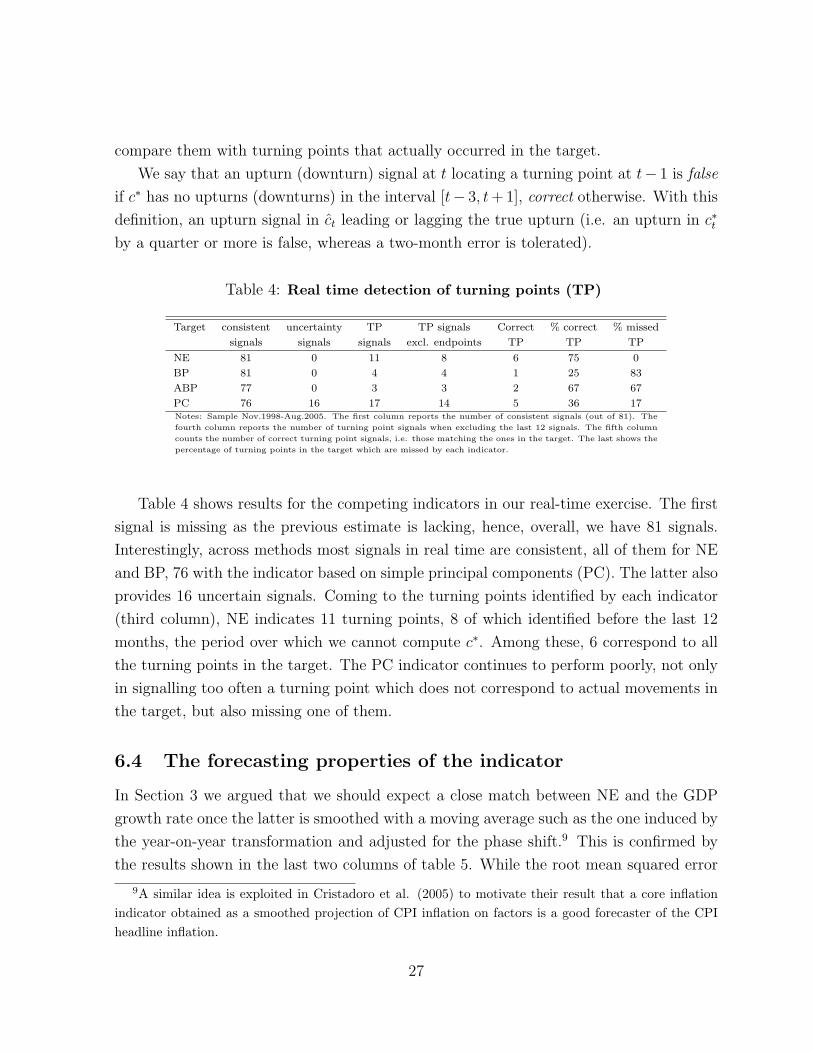
compare them with turning points that actually occurred in the target.
We say that an upturn (downturn) signal at t locating a turning point at t− 1 is false
if c∗ has no upturns (downturns) in the interval [t− 3, t+ 1], correct otherwise. With this
definition, an upturn signal in ct leading or lagging the true upturn (i.e. an upturn in c∗tby a quarter or more is false, whereas a two-month error is tolerated).
Table 4: Real time detection of turning points (TP)
Target consistent uncertainty TP TP signals Correct % correct % missed
signals signals signals excl. endpoints TP TP TP
NE 81 0 11 8 6 75 0
BP 81 0 4 4 1 25 83
ABP 77 0 3 3 2 67 67
PC 76 16 17 14 5 36 17Notes: Sample Nov.1998-Aug.2005. The first column reports the number of consistent signals (out of 81). The
fourth column reports the number of turning point signals when excluding the last 12 signals. The fifth column
counts the number of correct turning point signals, i.e. those matching the ones in the target. The last shows the
percentage of turning points in the target which are missed by each indicator.
Table 4 shows results for the competing indicators in our real-time exercise. The first
signal is missing as the previous estimate is lacking, hence, overall, we have 81 signals.
Interestingly, across methods most signals in real time are consistent, all of them for NE
and BP, 76 with the indicator based on simple principal components (PC). The latter also
provides 16 uncertain signals. Coming to the turning points identified by each indicator
(third column), NE indicates 11 turning points, 8 of which identified before the last 12
months, the period over which we cannot compute c∗. Among these, 6 correspond to all
the turning points in the target. The PC indicator continues to perform poorly, not only
in signalling too often a turning point which does not correspond to actual movements in
the target, but also missing one of them.
6.4 The forecasting properties of the indicator
In Section 3 we argued that we should expect a close match between NE and the GDP
growth rate once the latter is smoothed with a moving average such as the one induced by
the year-on-year transformation and adjusted for the phase shift.9 This is confirmed by
the results shown in the last two columns of table 5. While the root mean squared error
9A similar idea is exploited in Cristadoro et al. (2005) to motivate their result that a core inflationindicator obtained as a smoothed projection of CPI inflation on factors is a good forecaster of the CPIheadline inflation.
27
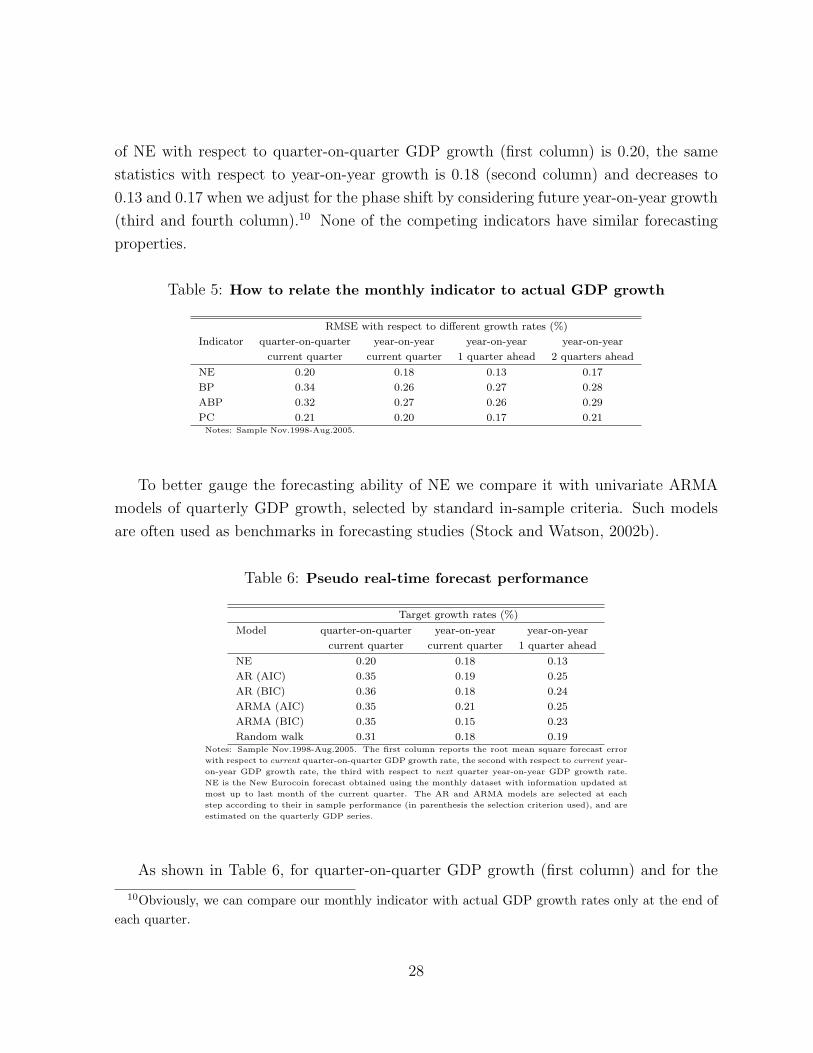
of NE with respect to quarter-on-quarter GDP growth (first column) is 0.20, the same
statistics with respect to year-on-year growth is 0.18 (second column) and decreases to
0.13 and 0.17 when we adjust for the phase shift by considering future year-on-year growth
(third and fourth column).10 None of the competing indicators have similar forecasting
properties.
Table 5: How to relate the monthly indicator to actual GDP growth
RMSE with respect to different growth rates (%)
Indicator quarter-on-quarter year-on-year year-on-year year-on-year
current quarter current quarter 1 quarter ahead 2 quarters ahead
NE 0.20 0.18 0.13 0.17
BP 0.34 0.26 0.27 0.28
ABP 0.32 0.27 0.26 0.29
PC 0.21 0.20 0.17 0.21Notes: Sample Nov.1998-Aug.2005.
To better gauge the forecasting ability of NE we compare it with univariate ARMA
models of quarterly GDP growth, selected by standard in-sample criteria. Such models
are often used as benchmarks in forecasting studies (Stock and Watson, 2002b).
Table 6: Pseudo real-time forecast performance
Target growth rates (%)
Model quarter-on-quarter year-on-year year-on-year
current quarter current quarter 1 quarter ahead
NE 0.20 0.18 0.13
AR (AIC) 0.35 0.19 0.25
AR (BIC) 0.36 0.18 0.24
ARMA (AIC) 0.35 0.21 0.25
ARMA (BIC) 0.35 0.15 0.23
Random walk 0.31 0.18 0.19Notes: Sample Nov.1998-Aug.2005. The first column reports the root mean square forecast error
with respect to current quarter-on-quarter GDP growth rate, the second with respect to current year-
on-year GDP growth rate, the third with respect to next quarter year-on-year GDP growth rate.
NE is the New Eurocoin forecast obtained using the monthly dataset with information updated at
most up to last month of the current quarter. The AR and ARMA models are selected at each
step according to their in sample performance (in parenthesis the selection criterion used), and are
estimated on the quarterly GDP series.
As shown in Table 6, for quarter-on-quarter GDP growth (first column) and for the
10Obviously, we can compare our monthly indicator with actual GDP growth rates only at the end ofeach quarter.
28

year-on-year growth rate one quarter ahead (third column) the forecast error of the indi-
cator is far lower than those obtained either with the ARMA or with the random walk.
7 Summary and conclusion
Our coincident indicator NE is a timely estimate of the medium to long-run component of
euro area GDP growth. The latter, our target, has been defined as a centred, symmetric
moving average of GDP growth, whose weights are designed to remove all fluctuations of
period shorter than one year. As observed in Section 3, the target, which has a rigorous
spectral definition, leads the “popular” measure of medium to long-run change, namely
year-on-year GDP growth, by several months.
We avoid the large end-of-sample bias typical of two-sided filters by projecting the
target onto suitable linear combinations of a large set of monthly variables. Such linear
combinations are designed to discard useless information, namely idiosyncratic and short-
run noise, and retain relevant information, i.e. common, cyclical and long-run waves.
Both the definition and the estimation of the common, medium to long-run waves are
based on recent factor model techniques. Embedding the smoothing into the construction
of the regressors is in our opinion an important contribution of the present paper.
The performance of NE as a real-time estimator of the target has been presented in
detail in Section 6. The indicator is smooth and easy to interpret. In terms of turn-
ing points detection, it scores much better than the competitors that naturally arise as
estimators of the medium to long-run component of GDP growth in real time. The re-
liability of the signal is reinforced by the fact that the revision error of our indicator is
extremely small compared with the competitors. We have also shown that NE is a very
good forecaster of year-on-year GDP growth 1 and 2 quarters ahead; it also scores well
in forecasting quarter-on-quarter GDP growth, with an RMSE of 0.20, which ranks well
even in comparison with best practice results.
29

Appendix A: Technical details
A.1 Computing c∗t
The approximation c∗t (T ) is obtained by
c∗t (T ) = µ+ β(L)Yt, (18)
where
µ =
bT/3c∑l=1
y3l−1/bT/3c (19)
and
Yt =
yt − µ for t = 3l − 1, 1 ≤ l ≤ bT/3c23y3l−1 + 1
3y3l+2 − µ for t = 3l, 1 ≤ l ≤ bT/3c − 1
13y3l−1 + 2
3y3l+2 − µ for t = 3l + 1, 1 ≤ l ≤ bT/3c − 1
0 for t < 1 and t > 3bT/3c − 1.
In words, Yt is obtained by centring (de-meaning) yt, filling the in-sample missing values
by linear interpolation and adding zeros outside the sample period. After applying β(L)
to Yt we add the estimated mean µ, so that the procedure is equivalent to (4). T denotes
the last observation available for our monthly series. Note that (18) takes into account
the publication delay of the GDP series described in Section 2.
The approximation c∗t is affected by two sources of errors.
(i) Firstly, as already observed in Section 3, our c∗t (T ) results from a t-dependent asym-
metric truncation of β(L). We can easily compute the approximation error under different
assumptions on yt. If yt is a white noise, for T = 215 the mean square approximation
error, normalized by the variance of ct, ranges from 0.6% for t in the middle of the sample,
to 2.6% for t = T −12. When we take T −81 as sample length, as we do at the beginning
of our pseudo real-time exercises, the corresponding figures are 0.9% and 2.7%. Note that
the case of a white noise is rather unfavourable. With a positive autocorrelated MA(1)
or AR(1), for example, we obtain slightly better results.
Asymmetry has also a phase-effect. This is independent of yt and can be easily com-
puted. Figure 8 shows the phase of the asymmetric truncation of β(L) at T − 12, the
worst case. More precisely, for each frequency between 0 and π/6, the figure shows the
ratio of the corresponding time delay to the length of the wave. For example, at frequency
0.2, which corresponds to a wave length of 2π/0.2 = 31.4 months, the phase delay does
30

0 0.1 0.2 0.3 0.4 0.5 0.6 0.7−0.12
−0.1
−0.08
−0.06
−0.04
−0.02
0
0.02
Figure 9: Phase delay at T − 12, as a function of the frequency between 0 and π/6
not reach 1%, that is about 0.3 months. It is only when the frequency approaches π/6
that the phase delay reaches 10%, that is 1.2 months.
(ii) Secondly, there is an error induced by linear interpolation. Again, the size of the error
depends on the unobservable autocorrelation structure of the original series. However,
this error is likely to be negligible. Our argument is based on some experiments. We take
a monthly series, compute its quarter-on-quarter growth rate zt, compute the linearly
interpolated series Zt (as though zt were not observable for two months out of each
quarter), and compare β(L)zt with β(L)Zt. For the industrial production index of the
euro zone we obtained a correlation coefficient of 0.9987. Similar results were obtained
for other series and by applying Chow and Lin’s method instead of linear interpolation.
This is hardly surprising. Our monthly quarter-on-quarter growth-rate series have by
construction a strong, positive autocorrelation at the first lags, due to overlapping (see
Section 2), so that linear interpolation, as well as Chow and Lin’s, should not be so far
from actual data. The remaining difference is made up of short-run oscillations that, as
already argued in Section 3, do not survive application of the filter β(L).
In conclusion, (a) At T − 12, i.e. in the worst situation, the approximation error and
31

the phase delay are negligible (the first never exceeds 3%), (b) experiments with actual
series show that linear interpolation does not make a significant difference on the result of
applying β(L) to quarter on quarter growth rates, so that c∗t may be taken as an extremely
good approximation of ct for the interval 13 ≤ t ≤ T − 12.
A.2 Estimating Σw and Σcw
As observed in the main text, estimation of Σw is trivial:
Σw =T∑t=1
wtw′t/(T − 1). (20)
Estimation of Σcw is less obvious, since ct is not observed. We proceed as follows. First,
we estimate the covariance of yt and wt at lags k = −M, . . . ,M as
Σyw(k) =∑l
y3l−1w′3l−1−k/(b(T − k)/3c − 1), (21)
where l varies from max[1, 1 + b(k + 1)/3c] to min[bT/3c, b(T − k)/3c]. Note that the
cross-covariances Σyw(k) can be consistently estimated for any lag k, despite the fact that
yt is only observed quarterly.
Then, we estimate the cross-spectrum over the relevant frequency interval, at the
2J + 1 equally spaced points θj, by using the Bartlett lag-window estimator
Syw(θj) =1
2π
M∑k=−M
Wk Σyw(k) e−iθjk, (22)
where Wk = 1 − |k|M+1
and θj = πj3(2J+1)
, j = −J, . . . , J . Note that the larger frequency
estimated is not π/6, but the middle point of the (2J + 1)-th interval, ending at π/6.
Finally, we estimate Σcw by averaging the cross-spectrum over such points, i.e.
Σcw =2π
2J + 1
J∑j=−J
Syw(θj). (23)
For New Eurocoin we set J = 60 and M = 24.
A.3 Estimating Σφ, Σχ and Σξ
To get an estimate of Σχ we have first to estimate the spectral density matrix of the
vector of monthly variables xt = (x1t · · · xnt)′. We estimate the covariance matrices of
32

xt at lags k = −M, . . . ,M , as
Σx(k) =∑t
xtx′t−k/(T − k),
where t varies from max[1, 1 + k] to min[T, T − k]. Then we estimate the spectrum of xt
at the 2J + 1 equally spaced frequencies θj by using the Bartlett lag-window estimator
Sx(θj) =1
2π
M∑l=−M
Wk Σx(k) e−iθjk, (24)
where Wk = 1 − |k|M+1
and θj = 2πj2J+1
, j = −J, . . . , J . Again we set J = 60 and M = 24.
As a second step, we compute the eigenvalues and eigenvectors of Sx(θ) at each fre-
quency. Let λj(θ) be the j-th largest eigenvalue of Sx(θ) and Uj(θ) be the corresponding
eigenvector. Moreover, let Λ(θ) be the q × q diagonal matrix having on the diagonal the
first q eigenvalues in descending order and U(θ) be the matrix having on the columns the
first q eigenvectors, i.e. U(θ) = [U1(θ)U2(θ) · · ·Uq(θ)]. Our estimate of Sχ is
Sχ(θ) = U(θ)Λ(θ)U(θ) (25)
where tilde denotes conjugation and transposition. Given the correct choice of q, consis-
tency results for the entries of this matrix as both n and T go to infinity can easily be
obtained from Forni, Hallin, Lippi and Reichlin (2000).
Third, we average Sχ(θ) over all points θj to get our estimate of Σχ and average Sχ(θ)
over the relevant frequency band [−2π12, 2π
12] to get our estimate of Σφ:
Σχ =2π
2J + 1
J∑j=−J
Sχ(θj); (26)
Σφ =2π
2J + 1
10∑j=−10
Sχ(θj). (27)
Finally, our estimate of the idiosyncratic variance-covariance matrix Σξ is simply ob-
tained as
Σξ = diag(Σx − Σχ
), (28)
diag(A) being the diagonal matrix obtained setting to zero the off-diagonal elements
of A. This operation is consistent with our assumption of mutual orthogonality of the
idiosyncratic components.
33

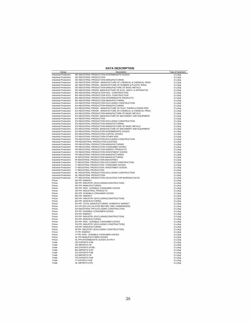
Appendix B: Dataset and treatment
The dataset includes 145 series from Thomson Financial Datastream, referring to the euro
area as well as its major economies. 11 For euro area GDP we used data from Fagan et
al. (2001) until the first quarter 1991, from then on we used the official Eurostat series
(rescaling data prior to 1992 to avoid a sudden change in level). The database is organized
into homogeneous blocks, i.e. industrial production indexes (41 series), prices (24), money
aggregates (8), interest rates (11), financial variables (6), demand indicators (14), surveys
(25), trade variables (9) and labour market series (7).
All series were transformed to remove outliers, seasonal factors and non-stationarity.
Regarding outliers, we eliminated from each series those points that were more than 5
standard deviation away from the mean and replaced them with the sample average of
the remaining observations. Seasonal adjustment was obtained by regressing variables on
a set of seasonal dummies. We did not resort to other more sophisticated procedures (e.g.
Seats or X12) to avoid the use of two-sided filters, which would potentially imply large
revisions in the seasonally adjusted series. Non-stationarity was removed following an
automatic procedure: all the series in a given economic class (e.g. industrial production,
prices and so on) were treated in the same way; unit root tests run afterwards confirmed
the reasonabless of this choice.
Finally, the series were normalized subtracting the mean and dividing for the standard
deviation as usually done in the large factor model literature. The detailed list of the
variables and the related transformation are reported in the table below.
11The final dataset used in this paper is the result of a search process in a much larger dataset ofeuro area and national variables. In particular, we looked for series satisfying three main criteria: (i) asufficient time series span (at least starting in 1987), (ii) with a high correlation and leading propertywith respect to GDP growth, (iii) released in timely manner by statistical agencies
34

References
[1] Altissimo, F., Bassanetti, A., Cristadoro, R., Forni, M., Hallin, M., Lippi, M., Reich-
lin, L. and Veronese, G. (2001). A real Time Coincident Indicator for the euro area
Business Cycle. CEPR Discussion Paper No. 3108.
[2] Anderson, T. W. (1984). An Introduction to Multivariate Statistical Analysis. New
York: John Wiley & Sons.
[3] Bai, J. (2003). Inferential theory for factor models of large dimension. Econometrica
71, 135-71.
[4] Bai, J. and S. Ng (2002). Determining the number of factors in approximate factor
models. Econometrica 70, 191-221.
[5] Baxter, A. and King, R.G. (1999). Measuring Business Cycle Approximate Band-
Pass filters for Economic Time Series. The Review of Economics and Statistics 81,
575-93.
[6] Bernanke, B. and Boivin, J. (2003). Monetary Policy in a Data-Rich Environment.
Journal of Monetary Economics 50:3, 525-46.
[7] Brockwell, P.J. and R. A. Davis (1991). Time Series: Theory and Methods. 2nd
Edition. New York: Springer-Verlag.
[8] Burns, A.F., and W.C. Mitchell (1946). Measuring Business Cycles. New York:
NBER.
[9] Chow, G.C. and Lin, A. (1971). Best Linear Unbiased Interpolation, Distribution,
and Extrapolation of Time Series by Related Time Series. The Review of Economics
and Statistics 53, 372-375.
[10] Christiano, L.J. and Fitzgerald, T.J. (2003). The Band-Pass Filter. International
Economic Review 84, 435-65.
[11] Cristadoro, R., Forni, M., Reichlin, L. and Veronese, G. (2005). A core inflation
indicator for the euro area, Journal of Money Credit and Banking 37(3), 539-560.
[12] Evans, M. (2005). Where Are We Now? Real-Time Estimates of the Macro Economy.
NBER WP Jan.2005.
35

[13] Fagan, G., J. Henry, and R. Mestre (2001). An area-wide-model (AWM) for the euro
area. ECB Working Paper Series no. 42.
[14] Forni, M., M. Hallin, M. Lippi, and L. Reichlin (2000). The generalized dynamic
factor model: identification and estimation. The Review of Economics and Statistics
82, 540-554.
[15] Forni, M., M. Hallin, M. Lippi, and L. Reichlin (2001). Coincident and leading indi-
cators for the euro area. The Economic Journal 111, 62-85.
[16] Forni, M., M. Hallin, M. Lippi, and L. Reichlin (2005). The generalized dynamic fac-
tor model: one-sided estimation and forecasting. Journal of the American Statistical
Association 100 830-40.
[17] Forni, M., M. Hallin, M. Lippi, and L. Reichlin (2004). The generalized dynamic
factor model: consistency and rates. Journal of Econometrics 119, 231-255.
[18] Forni, M. and M. Lippi (2001). The generalized dynamic factor model: representation
theory. Econometric Theory 17, 1113-41.
[19] Giannone, D., Reichlin, L. and Sala, L. (2002). Tracking Greenspan: Systematic and
Unsystematic Monetary Policy Revisited. CEPR Discussion Paper No. 3550.
[20] Hallin, M. and R. Liska (2007). Determining the Number of Factors in the Gener-
alized Factor Model, Journal of the American Statistical Association, 102, No. 478,
603-617.
[21] Kapetanios, G., M. Marcellino (2004). A parametric estimation method for dynamic
factor models of large dimensions. Queen Mary University of London Working Paper
489.
[22] Mitchell, J., Smith R., Weale M., Wright S. and Salazar E. (2004). An Indicator of
Monthly GDP and an Early Estimate of Quarterly GDP Growth. National Institute
of Economic and Social Research Discussion Paper.
[23] Pesaran, M.H. and A. Timmermann (1992). A Simple Non-Parametric Test of Pre-
dictive Performance. Journal of Business and Economics Statistics 4, pp. 461-465.
[24] Stock, J. H., and Watson, M. W. (1989). New Indexes of Coincident and Leading
Economic Indicators. NBER Macroeconomics Annual, pp. 351-393.
36

[25] Stock, J. H., and Watson, M. W. (1999). Business Cycle Fluctuations in U.S. Macroe-
conomic Time Series. In G. B. Taylor and M. Woodford (eds.), Handbook of Macroe-
conomics,pp. 3-64. Amsterdam: Elsevier Science Publishers.
[26] Stock, J.H. and M.W. Watson (2002a). Forecasting using principal components from
a large number of predictors. Journal of the American Statistical Association 97,
1167-79.
[27] Stock, J.H. and M.W. Watson (2002b). Macroeconomic forecasting using diffusion
indexes. Journal of Business and Economic Statistics 20, 147-162.
[28] Valle e Azevedo J., Koopman S.J., Rua A. (2006). Tracking the business cycle of
the euro area: a multivariate model-based band-pass filter. Journal of Business and
Economic Statistics, 24, 278-290.
[29] Zarnowitz, V. and Ozyildirim, A. (2002). Time series decomposition and measure-
ment of business cycles, trends and growth cycles. NBER WP No. 8736.
37
Group Description Type of treatmentIndustrial Production DE INDUSTRIAL PRODUCTION-INTERMEDIATE GOODS (1-L)logIndustrial Production DE INDUSTRIAL PRODUCTION (1-L)logIndustrial Production DE INDUSTRIAL PRODUCTION-MANUFACTURING (1-L)logIndustrial Production DE INDUSTRIAL PRODN - MANUFACTURE OF CHEMICAL & CHEMICAL PRDS. (1-L)logIndustrial Production DE INDUSTRIAL PRODN. -MANUFACTURE OF RUBBER & PLASTIC PRDS. (1-L)logIndustrial Production DE INDUSTRIAL PRODUCTION-MANUFACTURE OF BASIC METALS (1-L)logIndustrial Production DE INDUSTRIAL PRODN -MANUFACTURE OF ELEC. MACH. & APPARATUS (1-L)logIndustrial Production BG INDUSTRIAL PRODUCTION INCL. CONSTRUCTION (1-L)logIndustrial Production BG INDUSTRIAL PRODUCTION EXCL CONSTRUCTION (1-L)logIndustrial Production BG INDUSTRIAL PRODUCTION-INTERMEDIATE PRODUCTS (1-L)logIndustrial Production BG INDUSTRIAL PRODUCTION-MANUFACTURING (1-L)logIndustrial Production EA INDUSTRIAL PRODUCTION EXCLUDING CONSTRUCTION (1-L)logIndustrial Production EA INDUSTRIAL PRODUCTION-MANUFACTURING (1-L)logIndustrial Production EA INDUSTRIAL PRODN - MANUFACTURE OF PULP, PAPER & PAPER PRD. (1-L)logIndustrial Production EA INDUSTRIAL PRODN - MANUFACTURE OF CHEMICAL & CHEMICAL PRDS. (1-L)logIndustrial Production EA INDUSTRIAL PRODUCTION-MANUFACTURE OF BASIC METALS (1-L)logIndustrial Production EA INDUSTRIAL PRODN -MANUFACTURE OF MACHINERY AND EQUIPMENT (1-L)logIndustrial Production EA INDUSTRIAL PRODUCTION (1-L)logIndustrial Production ES INDUSTRIAL PRODUCTION EXCLUDING CONSTRUCTION (1-L)logIndustrial Production ES INDUSTRIAL PRODUCTION-MANUFACTURING (1-L)logIndustrial Production ES INDUSTRIAL PRODUCTION-MANUFACTURE OF BASIC METALS (1-L)logIndustrial Production ES INDUSTRIAL PRODN -MANUFACTURE OF MACHINERY AND EQUIPMENT (1-L)logIndustrial Production ES INDUSTRIAL PRODUCTION-INTERMEDIATE GOODS (1-L)logIndustrial Production ES INDUSTRIAL PRODUCTION-CAPITAL GOODS (1-L)logIndustrial Production ES INDUSTRIAL PRODUCTION-OTHER NON (1-L)logIndustrial Production FN INDUSTRIAL PRODUCTION EXCLUDING CONSTRUCTION (1-L)logIndustrial Production FR INDUDSTRIAL PRODUCTION (UUSTED) (1-L)logIndustrial Production FR INDUSTRIAL PRODUCTION-MANUFACTURING (1-L)logIndustrial Production FR INDUSTRIAL PRODUCTION-CONSUMER GOODS (1-L)logIndustrial Production FR INDUSTRIAL PRODUCTION-ENERGY PRODUCTS (1-L)logIndustrial Production FR INDUSTRIAL PRODUCTION-INVESTMENT GOODS (1-L)logIndustrial Production FR INDUSTRIAL PRODUCTION-MANUFACTURING (1-L)logIndustrial Production IR INDUSTRIAL PRODUCTION-MANUFACTURING (1-L)logIndustrial Production IR INDUSTRIAL PRODUCTION-INDUSTRIES (1-L)logIndustrial Production IT INDUSTRIAL PRODUCTION EXCLUDING CONSTRUCTION (1-L)logIndustrial Production IT INDUSTRIAL PRODUCTION: CONSUMER GOODS (1-L)logIndustrial Production IT INDUSTRIAL PRODUCTION: INVESTMENT GOODS (1-L)logIndustrial Production IT INDUSTRIAL PRODUCTION (1-L)logIndustrial Production NL INDUSTRIAL PRODUCTION EXCLUDING CONSTRUCTION (1-L)logIndustrial Production NL INDUSTRIAL PRODUCTION (1-L)logIndustrial Production PT INDUSTRIAL PRODUCTION (ADJUSTED FOR WORKING DAYS) (1-L)logPrices DE PPI: ENERGY (1-L)logPrices DE PPI: INDUSTRY (EXCLUDINGCONSTRUCTION) (1-L)logPrices DE PPI: MANUFACTURING (1-L)logPrices DE PPI: NON - DURABLE CONSUMER GOODS (1-L)logPrices DE PPI: INDUSTRIAL PRODUCTS (1-L)logPrices BG PPI: DURABLE CONSUMER GOODS (1-L)logPrices BG PPI: ENERGY (1-L)logPrices BG PPI: INDUSTRY (EXCLUDINGCONSTRUCTION) (1-L)logPrices BG PPI: MANUFACTURING (1-L)logPrices EA PPI: TOTAL MANUFACTURING -DOMESTIC MARKET (1-L)logPrices EA CPI (DS CALCULATED BEFORE 1990, HARMONISED) (1-L)logPrices EA INDUSTRIAL PPI-EXCLUDING CONSTRUCTION (1-L)logPrices ES PPI: DURABLE CONSUMER GOODS (1-L)logPrices ES PPI: ENERGY (1-L)logPrices ES PPI: INDUSTRY (EXCLUDINGCONSTRUCTION) (1-L)logPrices ES PPI: MANUFACTURING (1-L)logPrices ES PPI: NON - DURABLE CONSUMER GOODS (1-L)logPrices FN PPI: INDUSTRY (EXCLUDING CONSTRUCTION) (1-L)logPrices GR PPI: MANUFACTURING (1-L)logPrices IR PPI: INDUSTRY (EXCLUDING CONSTRUCTION) (1-L)logPrices IT PPI: ENERGY (1-L)logPrices IT PPI: NON - DURABLE CONSUMER GOODS (1-L)logPrices NL PPI-MANUFACTURED GOODS (1-L)logPrices NL PPI-INTERMEDIATE GOODS OUTPUT (1-L)logTrade DE EXPORTS FOB (1-L)logTrade DE IMPORTS CIF (1-L)logTrade BG EXPORTS (FOB) (1-L)logTrade BG IMPORTS (CIF) (1-L)logTrade ES EXPORTS FOB (1-L)logTrade ES IMPORTS CIF (1-L)logTrade FR EXPORTS FOB (1-L)logTrade IT EXPORTS FOB (1-L)logTrade NL IMPORTS (CIF) (1-L)log
DATA DESCRIPTION
38

Group Description Type of treatmentSurveys DE CONSUMER SURVEY: MAJOR PURCH.OVER NEXT 12 MONTHS - GERMANY --Surveys DE INDUSTRY SURVEY: ORDER BOOK POSITION-GERMANY --Surveys BG INDUSTRIAL CONFIDENCE INDICATOR-BELGIUM --Surveys BG INDUSTRY SURVEY: ORDER BOOK POSITION-BELGIUM --Surveys ES CONSUMER SURVEY: MAJOR PURCH.OVER NEXT 12 MONTHS-SPAIN --Surveys ES ECONOMIC SENTIMENT INDICATOR-SPAIN --Surveys ES INDUSTRY SURVEY: ORDER BOOK POSITION-SPAIN --Surveys ES INDUSTRY SURVEY: PROD.EXPECTATION FOR MTH. AHEAD-SPAIN --Surveys FR CONSTRUCTION CONFIDENCE INDICATOR-FRANCE --Surveys FR INDUSTRIAL CONFIDENCE INDICATOR-FRANCE --Surveys FR SURVEY: INDUSTRY-ORDERBOOK & DEMAND --Surveys FR SURVEY: MANUFACTURING OUTPUT LEVEL-GENERAL OUTLOOK --Surveys FR SURVEY: INDUSTRY-RECENT OUTPUT TREND --Surveys FR SURVEY: INDUSTRY-PROBABLE OUTPUT TREND --Surveys IT ISAE HOUSEHOLD CONFIDENCE INDEX: NET OF IRREGULAR COMPONENTS --Surveys IT CONSUMER CONFIDENCE INDICATOR-ITALY --Surveys IT INDUSTRY SURVEY: STOCKS OF FINISHED GOODS-ITALY --Surveys IT INDUSTRY SURVEY: PROD.EXPECTATION FOR MTH. AHEAD-ITALY --Surveys NL CONSUMER SURVEY: ECONOMIC SITUATION LAST 12 MTH - NETHERLANDS --Surveys DE ASSESSMENT OF BUSINESS SITUATION: CONSTRUCTION --Surveys DE ASSESSMENT OF BUSINESS SITUATION --Surveys DE BUSINESS EXPECTATIONS --Surveys DE ASSESSMENT OF BUSINESS SITUATION: MANUFACTURING --Surveys DE BUSINESS CLIMATE INDEX: MANUFACTURING --Surveys DE ASSESSMENT OF BUSINESS SITUATION: TRADE --Interest Rates DE MONEY MARKET RATE ( FEDERAL FUNDS ) (1-L)Interest Rates DE GOVT BOND YIELD-LONGTERM (1-L)Interest Rates DE MORTGAGE BANK LENDING TODOMESTIC NON - BANKS (1-L)logInterest Rates BG CENTRAL GOVERNMENT BOND-5 YEAR YIELD --Interest Rates BG TREASURY BILL RATE (1-L)Interest Rates FN MONEY MARKET RATE ( FEDERAL FUNDS ) (1-L)Interest Rates FR MONEY MARKET INT.RATES -AVERAGE YEARLY MONEY MARKET RATE (1-L)Interest Rates GR TREASURY BILL RATE (1-L)Interest Rates IT TREASURY BOND NET YIELD- SECONDARY MKT. (EP) (1-L)Interest Rates NL LENDING RATE (PRIME RATE) (1-L)Interest Rates NL GOVT BOND YIELD-LONGTERM (1-L)Wages DE UNIT LABOUR COSTS, RELATIVE NORMALIZED (1-L)logWages DE WAGE & SALARY RATES: MONTHLY - PRODUCING SECTOR(PAN DE M0191) (1-L)logWages IT HOURLY RATES IN INDUSTRY (1-L)logWages NL HOURLY WAGE RATE MANUFACTURING (1-L)logMoney Supply DE MONEY SUPPLY-M2 (CONTINUOUS SERIES) (1-L)logMoney Supply DE MONEY SUPPLY-M3 (CONTINUOUS SERIES) (1-L)logMoney Supply EA MONEY SUPPLY: M1 (1-L)logMoney Supply EA MONEY SUPPLY: M3 (1-L)logMoney Supply FR MONEY SUPPLY-M1 (NATIONAL CONTRIBUTION TO M1) (1-L)logMoney Supply FR MONEY SUPPLY-M3 (NATIONAL CONTRIBUTION TO M3) (1-L)logMoney Supply IT MONEY SUPPLY: M1-ITALIAN CONTRIBUTION TO THE EURO AREA (1-L)logMoney Supply IT MONEY SUPPLY: M3-ITALIAN CONTRIBUTION TO THE EURO AREA (1-L)logExchange Rates DE REAL EFFECTIVE EXCHANGE RATES (1-L)Exchange Rates EA U.S. $ TO 1 EURO (ECU PRIOR TO 1999) (1-L)Exchange Rates IT REAL EFFECTIVE EXCHANGE RATES (1-L)Finance FR SHARE PRICES-SBF 250 (1-L)logFinance US STANDARD AND POORS COMPOSITE INDEX (EP) (1-L)logFinance US DOW JONES INDUSTRIALS SHARE PRICE INDEX (EP) (1-L)logDemand Indicators DE RETAIL SALES EXCLUDING CARS (DERETT0TF FOR 2000=100) (1-L)logDemand Indicators DE VACANCIES (PAN DE FROM JAN 1994) (1-L)Demand Indicators DE WHOLE SALES TURN OVER, NOMINAL VALUE (1-L)logDemand Indicators BG NEW CAR REGISTRATIONS (1-L)logDemand Indicators BG RETAIL SALES (1-L)logDemand Indicators BG RETAIL SALES-FOOD (1-L)logDemand Indicators ES EMPLOYMENT PROMOTION CONTRACTS: IN PRACTICE (1-L)Demand Indicators ES NEW CAR REGISTRATIONS (1-L)logDemand Indicators FR NEW CAR REGISTRATIONS (1-L)logDemand Indicators FR HOUSEHOLD CONSUMPTION-DURABLE GOODS (1-L)logDemand Indicators FR HOUSEHOLD CONSUMPTION-MANUFACTURED GOODS, RETAIL GOODS (1-L)logDemand Indicators FR HOUSEHOLD CONSUMPTION-MANUFACTURED GOODS (1-L)logDemand Indicators IT NEW CAR REGISTRATIONS (1-L)logDemand Indicators IT RETAIL SALES (1-L)logUnemployment DE STANDARDIZED UNEMPLOYMENT RATE (1-L)Unemployment FR UNEMPLOYMENT RATE-UNDER 25 YEARS (1-L)Unemployment IR STANDARDIZED UNEMPLOYMENT RATE (1-L)
DATA DESCRIPTION (continued )
39

(*) Requests for copies should be sent to: Banca d’Italia – Servizio Studi – Divisione Biblioteca e pubblicazioni – Via Nazionale, 91 – 00184 Rome(fax 0039 06 47922059). They are available on the Internet www.bancaditalia.it.
RECENTLY PUBLISHED “TEMI” (*)
N. 607 – What does a technology shock do? A VAR analysis with model-based sign restrictions, by L. Dedola and S. Neri (December 2006).
N. 608 – Merge and compete: Strategic incentives for vertical integration, by Filippo Vergara Caffarelli (December 2006).
N. 609 – Real-time determinants of fiscal policies in the euro area: Fiscal rules, cyclical conditions and elections, by Roberto Golinelli and Sandro Momigliano (December 2006).
N. 610 – L’under-reporting della ricchezza finanziaria nell’indagine sui bilanci delle famiglie, by Leandro D’Aurizio, Ivan Faiella, Stefano Iezzi, Andrea Neri (December 2006).
N. 611 – La polarizzazione territoriale del prodotto pro capite: un’analisi del caso italiano sulla base di dati provinciali by Stefano Iezzi (December 2006).
N. 612 – A neural network architecture for data editing in the Bank of Italy’s business surveys by Claudia Biancotti, Leandro D’Aurizio and Raffaele Tartaglia-Polcini (February 2007).
N. 613 – Outward FDI and Local Employment Growth in Italy, by Stefano Federico and Gaetano Alfredo Minerva (February 2007).
N. 614 – Testing for trend, by Fabio Busetti and Andrew Harvey (February 2007).N. 615 – Macroeconomic uncertainty and banks’ lending decisions: The case of Italy, by
Mario Quagliariello (February 2007).N. 616 – Entry barriers in italian retail trade, by Fabiano Schivardi and Eliana Viviano
(February 2007).N. 617 – A politicy-sensible core-inflation measure for the euro area, by Stefano Siviero and
Giovanni Veronese (February 2007).N. 618 – Le opinioni degli italiani sull’evasione fiscale, by Luigi Cannari and Giovanni
D'Alessio (February 2007)N. 619 – Memory for prices and the euro cash changeover: An analysis for cinema prices in
Italy, by Vincenzo Cestari, Paolo Del Giovane and Clelia Rossi-Arnaud (February 2007).
N. 620 – Intertemporal consumption choices, transaction costs and limited participation in financial markets: Reconciling data and theory, by Orazio P. Attanasio and Monica Paiella (April 2007).
N. 621 – Why demand uncertainty curbs investment: Evidence from a panel of Italian manufacturing firms, by Maria Elena Bontempi, Roberto Golinelli and Giuseppe Parigi (April 2007).
N. 622 – Employment, innovation and productivity: Evidence from Italian microdata, by Bronwyn H. Hall, Francesca Lotti and Jacques Mairesse (April 2007).
N. 623 – Measurement of Income Distribution in Supranational Entities: The Case of the European Union, by Andrea Brandolini (April 2007).
N. 624 – Un nuovo metodo per misurare la dotazione territoriale di infrastrutture di trasporto, by Giovanna Messina (April 2007).
N. 625 – The forgone gains of incomplete portfolios, by Monica Paiella (April 2007).N. 626 – University drop-out: The case of Italy, by Federico Cingano and Piero Cipollone
(April 2007).N. 627 – The sectoral distribution of money supply in the euro area, by Giuseppe Ferrero,
Andrea Nobili and Patrizia Passiglia (April 2007).N. 628 – Changes in transport and non-transport costs: Local vs global impacts in a spatial
network, by Kristian Behrens, Andrea R. Lamorgese, Gianmarco I.P. Ottaviano and Takatoshi Tabuchi (April 2007).
N. 629 – Monetary policy shocks in the euro area and global liquidity spillovers, by João Sousa and Andrea Zaghini (June 2007).
N. 630 – Endogenous growth and trade liberalization between asymmetric countries, by Daniela Marconi (June 2007).

"TEMI" LATER PUBLISHED ELSEWHERE
2004
P. ANGELINI and N. CETORELLI, Gli effetti delle modifiche normative sulla concorrenza nel mercato creditizio, in F. Panetta (eds.), Il sistema bancario negli anni novanta: gli effetti di una trasformazione, Bologna, il Mulino, TD No. 380 (October 2000).
P. CHIADES and L. GAMBACORTA, The Bernanke and Blinder model in an open economy: The Italian case, German Economic Review, Vol. 5 (1), pp. 1-34, TD No. 388 (December 2000).
M. BUGAMELLI and P. PAGANO, Barriers to investment in ICT, Applied Economics, Vol. 36 (20), pp. 2275-2286, TD No. 420 (October 2001).
F. BUSETTI, Preliminary data and econometric forecasting: An application with the Bank of Italy quarterly model, CEPR Discussion Paper, 4382, TD No. 437 (December 2001).
A. BAFFIGI, R. GOLINELLI and G. PARIGI, Bridge models to forecast the euro area GDP, International Journal of Forecasting, Vol. 20 (3), pp. 447-460,TD No. 456 (December 2002).
D. AMEL, C. BARNES, F. PANETTA and C. SALLEO, Consolidation and efficiency in the financial sector: A review of the international evidence, Journal of Banking and Finance, Vol. 28 (10), pp. 2493-2519, TD No. 464 (December 2002).
M. PAIELLA, Heterogeneity in financial market participation: Appraising its implications for the C-CAPM, Review of Finance, Vol. 8, 3, pp. 445-480, TD No. 473 (June 2003).
F. CINGANO and F. SCHIVARDI, Identifying the sources of local productivity growth, Journal of the European Economic Association, Vol. 2 (4), pp. 720-742, TD No. 474 (June 2003).
E. BARUCCI, C. IMPENNA and R. RENÒ, Monetary integration, markets and regulation, Research in Banking and Finance, (4), pp. 319-360, TD No. 475 (June 2003).
G. ARDIZZI, Cost efficiency in the retail payment networks: first evidence from the Italian credit card system, Rivista di Politica Economica, Vol. 94, (3), pp. 51-82, TD No. 480 (June 2003).
E. BONACCORSI DI PATTI and G. DELL’ARICCIA, Bank competition and firm creation, Journal of Money Credit and Banking, Vol. 36 (2), pp. 225-251, TD No. 481 (June 2003).
R. GOLINELLI and G. PARIGI, Consumer sentiment and economic activity: a cross country comparison, Journal of Business Cycle Measurement and Analysis, Vol. 1 (2), pp. 147-170, TD No. 484 (September 2003).
L. GAMBACORTA and P. E. MISTRULLI, Does bank capital affect lending behavior?, Journal of Financial Intermediation, Vol. 13 (4), pp. 436-457, TD No. 486 (September 2003).
F. SPADAFORA, Il pilastro privato del sistema previdenziale: il caso del Regno Unito, Economia Pubblica, 34, (5), pp. 75-114, TD No. 503 (June 2004).
F. LIPPI. and S. NERI, Information variables for monetary policy in a small structural model of the euro area, Journal of Monetary Economics, v. 54, 4, pp. 1256-1270, TD No. 511 (July 2004).
C. BENTIVOGLI and F. QUINTILIANI, Tecnologia e dinamica dei vantaggi comparati: un confronto fra quattro regioni italiane, in C. Conigliani (eds.), Tra sviluppo e stagnazione: l’economia dell’Emilia-Romagna, Bologna, Il Mulino, TD No. 522 (October 2004).
G. GOBBI and F. LOTTI, Entry decisions and adverse selection: An empirical analysis of local credit markets, Journal of Financial services Research, Vol. 26 (3), pp. 225-244, TD No. 535 (December 2004).
E. GAIOTTI and F. LIPPI, Pricing behavior and the introduction of the euro: Evidence from a panel of restaurants, Giornale degli Economisti e Annali di Economia, 2004, Vol. 63, (3/4), pp. 491-526, TD No. 541 (February 2005).
A. CICCONE, F. CINGANO and P. CIPOLLONE, The private and social return to schooling in Italy, Giornale degli economisti e annali di economia, v. 63, 3-4, pp. 413-444, TD No. 569 (January 2006).

2005
L. DEDOLA and F. LIPPI, The monetary transmission mechanism: Evidence from the industries of 5 OECD countries, European Economic Review, 2005, Vol. 49, (6), pp. 1543-1569, TD No. 389 (December 2000).
D. Jr. MARCHETTI and F. NUCCI, Price stickiness and the contractionary effects of technology shocks. European Economic Review, v. 49, pp. 1137-1164, TD No. 392 (February 2001).
G. CORSETTI, M. PERICOLI and M. SBRACIA, Some contagion, some interdependence: More pitfalls in tests of financial contagion, Journal of International Money and Finance, v. 24, 8, pp. 1177-1199, TD No. 408 (June 2001).
GUISO L., L. PISTAFERRI and F. SCHIVARDI, Insurance within the firm. Journal of Political Economy, 113, pp. 1054-1087, TD No. 414 (August 2001)
R. CRISTADORO, M. FORNI, L. REICHLIN and G. VERONESE, A core inflation indicator for the euro area, Journal of Money, Credit, and Banking, v. 37, 3, pp. 539-560, TD No. 435 (December 2001).
F. ALTISSIMO, E. GAIOTTI and A. LOCARNO, Is money informative? Evidence from a large model used for policy analysis, Economic & Financial Modelling, v. 22, 2, pp. 285-304, TD No. 445 (July 2002).
G. DE BLASIO and S. DI ADDARIO, Do workers benefit from industrial agglomeration? Journal of regional Science, Vol. 45, (4), pp. 797-827, TD No. 453 (October 2002).
R. TORRINI, Cross-country differences in self-employment rates: The role of institutions, Labour Economics, V. 12, 5, pp. 661-683, TD No. 459 (December 2002).
A. CUKIERMAN and F. LIPPI, Endogenous monetary policy with unobserved potential output, Journal of Economic Dynamics and Control, v. 29, 11, pp. 1951-1983, TD No. 493 (June 2004).
M. OMICCIOLI, Il credito commerciale: problemi e teorie, in L. Cannari, S. Chiri e M. Omiccioli (eds.), Imprese o intermediari? Aspetti finanziari e commerciali del credito tra imprese in Italia, Bologna, Il Mulino, TD No. 494 (June 2004).
L. CANNARI, S. CHIRI and M. OMICCIOLI, Condizioni di pagamento e differenziazione della clientela, in L. Cannari, S. Chiri e M. Omiccioli (eds.), Imprese o intermediari? Aspetti finanziari e commerciali del credito tra imprese in Italia, Bologna, Il Mulino, TD No. 495 (June 2004).
P. FINALDI RUSSO and L. LEVA, Il debito commerciale in Italia: quanto contano le motivazioni finanziarie?, in L. Cannari, S. Chiri e M. Omiccioli (eds.), Imprese o intermediari? Aspetti finanziari e commerciali del credito tra imprese in Italia, Bologna, Il Mulino, TD No. 496 (June 2004).
A. CARMIGNANI, Funzionamento della giustizia civile e struttura finanziaria delle imprese: il ruolo del credito commerciale, in L. Cannari, S. Chiri e M. Omiccioli (eds.), Imprese o intermediari? Aspetti finanziari e commerciali del credito tra imprese in Italia, Bologna, Il Mulino, TD No. 497 (June 2004).
G. DE BLASIO, Credito commerciale e politica monetaria: una verifica basata sull’investimento in scorte, in L. Cannari, S. Chiri e M. Omiccioli (eds.), Imprese o intermediari? Aspetti finanziari e commerciali del credito tra imprese in Italia, Bologna, Il Mulino, TD No. 498 (June 2004).
G. DE BLASIO, Does trade credit substitute bank credit? Evidence from firm-level data. Economic notes, Vol. 34 (1), pp. 85-112, TD No. 498 (June 2004).
A. DI CESARE, Estimating expectations of shocks using option prices, The ICFAI Journal of Derivatives Markets, Vol. 2, (1), pp. 42-53, TD No. 506 (July 2004).
M. BENVENUTI and M. GALLO, Il ricorso al "factoring" da parte delle imprese italiane, in L. Cannari, S. Chiri e M. Omiccioli (eds.), Imprese o intermediari? Aspetti finanziari e commerciali del credito tra imprese in Italia, Bologna, Il Mulino, TD No. 518 (October 2004).
L. CASOLARO and L. GAMBACORTA, Redditività bancaria e ciclo economico, Bancaria, v. 61, 3, pp. 19-27, TD No. 519 (October 2004).
F. PANETTA, F. SCHIVARDI and M. SHUM, Do mergers improve information? Evidence from the loan market, CEPR Discussion Paper, 4961, TD No. 521 (October 2004).
P. DEL GIOVANE and R. SABBATINI, La divergenza tra inflazione rilevata e percepita in Italia, Bologna, Il Mulino, TD No. 532 (December 2004).
R. TORRINI, Quota dei profitti e redditività del capitale in Italia: un tentativo di interpretazione, Politica economica, v. 21, pp. 7-42, TD No. 551 (June 2005).
M. OMICCIOLI, Il credito commerciale come “collateral”, in L. Cannari, S. Chiri, M. Omiccioli (eds.), Imprese o intermediari? Aspetti finanziari e commerciali del credito tra imprese in Italia, Bologna, il Mulino, TD No. 553 (June 2005).

L. CASOLARO, L. GAMBACORTA and L. GUISO, Regulation, formal and informal enforcement and the development of the household loan market. Lessons from Italy, in Bertola G., Grant C. and Disney R. (eds.) The Economics of Consumer Credit: European Experience and Lessons from the US, Boston, MIT Press, TD No. 560 (September 2005).
P. ANGELINI and F. LIPPI, Did inflation really soar after the euro changeover? Indirect evidence from ATM withdrawals, CEPR Discussion Paper, 4950, TD No. 581 (March 2006).
S. DI ADDARIO, Job search in thick markets: Evidence from Italy, Oxford Discussion Paper 235, Department of Economics Series, TD No. 605 (December 2006).
2006
F. BUSETTI, Tests of seasonal integration and cointegration in multivariate unobserved component models, Journal of Applied Econometrics, v. 21, 4, pp. 419-438, TD No. 476 (June 2003).
C. BIANCOTTI, A polarization of inequality? The distribution of national Gini coefficients 1970-1996, Journal of Economic Inequality, v. 4, 1, pp. 1-32, TD No. 487 (March 2004).
L. CANNARI and S. CHIRI, La bilancia dei pagamenti di parte corrente Nord-Sud (1998-2000), in L. Cannari, F. Panetta (a cura di), Il sistema finanziario e il Mezzogiorno: squilibri strutturali e divari finanziari, Bari, Cacucci, TD No. 490 (March 2004).
M. BOFONDI and G. GOBBI, Information barriers to entry into credit markets, Review of Finance, Vol. 10 (1), pp. 39-67, TD No. 509 (July 2004).
LIPPI F. and W. FUCHS, Monetary union with voluntary participation, Review of Economic Studies, 73, pp. 437-457 TD No. 512 (July 2004).
GAIOTTI E. and A. SECCHI, Is there a cost channel of monetary transmission? An investigation into the pricing behaviour of 2000 firms, Journal of Money, Credit, and Banking, v. 38, 8, pp. 2013-2038 TD No. 525 (December 2004).
A. BRANDOLINI, P. CIPOLLONE and E. VIVIANO, Does the ILO definition capture all unemployment?, Journal of the European Economic Association, v. 4, 1, pp. 153-179, TD No. 529 (December 2004).
A. BRANDOLINI, L. CANNARI, G. D’ALESSIO and I. FAIELLA, Household wealth distribution in Italy in the 1990s, In E. N. Wolff (ed.) International Perspectives on Household Wealth, Cheltenham, Edward Elgar, TD No. 530 (December 2004).
P. DEL GIOVANE and R. SABBATINI, Perceived and measured inflation after the launch of the Euro: Explaining the gap in Italy, Giornale degli economisti e annali di economia, v. 65, 2 , pp. 155-192, TD No. 532 (December 2004).
M. CARUSO, Monetary policy impulses, local output and the transmission mechanism, Giornale degli economisti e annali di economia, v. 65, 1, pp. 1-30, TD No. 537 (December 2004).
L. GUISO and M. PAIELLA, The role of risk aversion in predicting individual behavior, In P. A. Chiappori e C. Gollier (eds.) Competitive Failures in Insurance Markets: Theory and Policy Implications, Monaco, CESifo, TD No. 546 (February 2005).
G. M. TOMAT, Prices product differentiation and quality measurement: A comparison between hedonic and matched model methods, Research in Economics, No. 60, pp. 54-68, TD No. 547 (February 2005).
F. LOTTI, E. SANTARELLI and M. VIVARELLI, Gibrat's law in a medium-technology industry: Empirical evidence for Italy, in E. Santarelli (ed.), Entrepreneurship, Growth, and Innovation: the Dynamics of Firms and Industries, New York, Springer, TD No. 555 (June 2005).
F. BUSETTI, S. FABIANI and A. HARVEY, Convergence of prices and rates of inflation, Oxford Bulletin of Economics and Statistics, v. 68, 1, pp. 863-878, TD No. 575 (February 2006).
M. CARUSO, Stock market fluctuations and money demand in Italy, 1913 - 2003, Economic Notes, v. 35, 1, pp. 1-47, TD No. 576 (February 2006).
S. IRANZO, F. SCHIVARDI and E. TOSETTI, Skill dispersion and productivity: An analysis with matched data, CEPR Discussion Paper, 5539, TD No. 577 (February 2006).
M. BUGAMELLI and A. ROSOLIA, Produttività e concorrenza estera, Rivista di politica economica, 3, TD No. 578 (February 2006).
R. BRONZINI and G. DE BLASIO, Evaluating the impact of investment incentives: The case of Italy’s Law 488/92. Journal of Urban Economics, vol. 60, n. 2, pag. 327-349, TD No. 582 (March 2006).
A. DI CESARE, Do market-based indicators anticipate rating agencies? Evidence for international banks, Economic Notes, v. 35, pp. 121-150, TD No. 593 (May 2006).

L. DEDOLA and S. NERI, What does a technology shock do? A VAR analysis with model-based sign restrictions, Journal of Monetary Economics, v. 54, 2, pp. 512 - 549, TD No. 607 (December 2006).
R. GOLINELLI and S. MOMIGLIANO, Real-time determinants of fiscal policies in the euro area, Journal of Policy Modeling, v. 28, 9, pp. 943-64, TD No. 609 (December 2006).
P. ANGELINI, S. GERLACH, G. GRANDE, A. LEVY, F. PANETTA, R. PERLI,S. RAMASWAMY, M. SCATIGNA
and P. YESIN, The recent behaviour of financial market volatility, BIS Papers, 29, QEF No. 2 (August 2006).
2007
S. DI ADDARIO and E. PATACCHINI, Wages and the city. Evidence from Italy, Development Studies Working Papers 231, Centro Studi Luca d’Agliano, TD No. 570 (January 2006).
F. LOTTI and J. MARCUCCI, Revisiting the empirical evidence on firms' money demand, Journal of Economics and Business, v. 59, 1, pp. 51-73, TD No. 595 (May 2006).
L. MONTEFORTE, Aggregation bias in macro models: Does it matter for the euro area?, Economic Modelling, 24, pp. 236-261, TD No. 534 (December 2004).
FORTHCOMING
P. ANGELINI, Liquidity and announcement effects in the euro area, Giornale degli economisti e annali di economia, TD No. 451 (October 2002).
S. MAGRI, Italian households' debt: The participation to the debt market and the size of the loan, Empirical Economics, TD No. 454 (October 2002).
G. FERRERO, Monetary policy, learning and the speed of convergence, Journal of Economic Dynamics and Control, TD No. 499 (June 2004).
M. PAIELLA, Does wealth affect consumption? Evidence for Italy, Journal of Macroeconomics, v. 29, 1, TD No. 510 (July 2004).
A. ANZUINI and A. LEVY, Monetary policy shocks in the new EU members: A VAR approach, Applied Economics TD No. 514 (July 2004).
S. MOMIGLIANO, J. Henry and P. Hernández de Cos, The impact of government budget on prices: Evidence from macroeconometric models, Journal of Policy Modelling, TD No. 523 (October 2004).
D. Jr. MARCHETTI and F. Nucci, Pricing behavior and the response of hours to productivity shocks, Journal of Money Credit and Banking, TD No. 524 (December 2004).
R. BRONZINI, FDI Inflows, Agglomeration and host country firms’ size: Evidence from Italy, Regional Studies, TD No. 526 (December 2004).
A. NOBILI, Assessing the predictive power of financial spreads in the euro area: does parameters instability matter?, Empirical Economics, v. 31, 4, pp. , TD No. 544 (February 2005).
P. ANGELINI and A. Generale, On the evolution of firm size distributions, American Economic Review, TD No. 549 (June 2005).
A. DALMAZZO and G. DE BLASIO, Production and consumption externalities of human capital: An empirical study for Italy, Journal of Population Economics, TD No. 554 (June 2005).
R. FELICI and M. PAGNINI,, Distance, bank heterogeneity and entry in local banking markets, The Journal of Industrial Economics, TD No. 557 (June 2005).
R. BRONZINI and G. DE BLASIO, Una valutazione degli incentivi pubblici agli investimenti, Rivista Italiana degli Economisti , TD No. 582 (March 2006).
P. CIPOLLONE and A. ROSOLIA, Social interactions in high school: Lessons from an earthquake, American Economic Review, TD No. 596 (September 2006).
F. BUSETTI and A. HARVEY, Testing for trend, Econometric Theory TD No. 614 (February 2007).