Temi di discussionedel Servizio Studi

Estimating state price densities by Hermite polynomials:theory and application to the Italian derivatives market

Number 507 - July 2004

by Paolo Guasoni

The purpose of the Temi di discussione series is to promote the circulation of workingpapers prepared within the Bank of Italy or presented in Bank seminars by outsideeconomists with the aim of stimulating comments and suggestions.

The views expressed in the articles are those of the authors and do not involve theresponsibility of the Bank.

Editorial Board:STEFANO SIVIERO, EMILIA BONACCORSI DI PATTI, FABIO BUSETTI, ANDREA LAMORGESE, MONICA PAIELLA, FRANCESCO PATERNÒ, MARCELLO PERICOLI, ALFONSO ROSOLIA, STEFANIA ZOTTERI, RAFFAELA BISCEGLIA (Editorial Assistant).

ESTIMATING STATE PRICE DENSITIES BY HERMITEPOLYNOMIALS: THEORY AND APPLICATION TO

THE ITALIAN DERIVATIVES MARKET

by Paolo Guasoni*

Abstract

We study the problem of extracting the state price densities from the marketprices of listed options.

Adapting a model of Madan and Milne to a multiple expiration setting, wepresent an estimation method for the risk-neutral probability at a moving horizonof fixed length. With the exception of volatility, all model parameters can be esti-mated by linear regression and their number can be chosen arbitrarily, dependingon the size of the dataset.

We discuss empirical issues related to the application of this model to real dataand show results on listed options on the Italian MIB30 equity index.

JEL classification: G12,G13.

Keywords: option pricing, state-price densities, orthogonal polynomials,risk-neutral valuation, calibration.

Contents

1. Introduction . . . . . . . . . . . . . . . . . . . . . . . . . . . . . . . . . . . . . . . . . . . . . . . . . . . . . . . 72. The Model . . . . . . . . . . . . . . . . . . . . . . . . . . . . . . . . . . . . . . . . . . . . . . . . . . . . . . . . 93. Multiple expirations . . . . . . . . . . . . . . . . . . . . . . . . . . . . . . . . . . . . . . . . . . . . . . .134. Application to Italian derivatives market . . . . . . . . . . . . . . . . . . . . . . . . . . . . . 154.1. Data . . . . . . . . . . . . . . . . . . . . . . . . . . . . . . . . . . . . . . . . . . . . . . . . . . . . . . . . . . . 154.2. Methodology . . . . . . . . . . . . . . . . . . . . . . . . . . . . . . . . . . . . . . . . . . . . . . . . . . . 154.3. Numerical results . . . . . . . . . . . . . . . . . . . . . . . . . . . . . . . . . . . . . . . . . . . . . . . .19References . . . . . . . . . . . . . . . . . . . . . . . . . . . . . . . . . . . . . . . . . . . . . . . . . . . . . . . . . .2 5

*Universita di Pisa, Dipartimento di Matematica and Boston University.

1 Introduction1 In modern finance theory usual financial instruments are seen as combi-nationsof elementary Arrow-Debreu securities and asset prices can be obtained as ex-pected values of their future payoff under a state-price (or risk-neutral) densityQ.

In general,Q is unique only if the market is complete and in this case optionprices are exactly determined by the no-arbitrage condition. On the contrary, in amarket with incomplete information there are infinitely many risk-neutral proba-bilities, each of them reflecting a particular attitude to risk.

Knowledge ofQ can be relevant for a number of applications, ranging fromthe pricing of unlisted derivatives (such as OTC contracts) to risk management.From the point of view of a regulator, knowledge of the risk-neutral probabilityQcan be useful in combination with that of the physical probabilityP , as it allowsthe time change of risk aversion in the market to be monitored. In view of theseapplications, the natural question is whether we can recover the marginal distribu-tion of an underlying assetS underQ from the observation of option prices.

Several methods have been proposed in the literature for this purpose: a firstapproach consists in modeling the dynamics of the underlying asset underQ sothat risk-neutral densities can be written in parametric form. This case encom-passes the stochastic volatility models of Heston [3] and Stein and Stein [7], aswell as several others with deterministic volatility. In a few simple cases, thismethod is particularly flexible and easy to implement, but in general it raises anumber of issues:

• it is heavily model-dependent since it requires ana priori specification of astochastic process for the asset price;

• for complex processes, the risk-neutral densities do not admit closed-formexpressions and numerical solutions of PDEs or simulation algorithms mustbe employed;

• when several multiple parameters appear in a joint minimization problem itis necessary to devise an estimation algorithm that avoids local minima.

1The first draft of this paper was completed while the author was affiliated to the ResearchDepartment of the Bank of Italy. The author wishes to thank Gur Huberman, Roberto Violi andGiuseppe Grande for stimulating discussions and for carefully reading earlier versions of the paper.This paper benefited from comments of seminar participants at the Bank of Italy and at the IIIWorkshop in Quantitative Finance held in Verona (2002). All remaining errors are the author’sresponsibility. Special thanks go Borsa Italiana SpA for kindly providing the options dataset.

The views expressed herein are those of the author and not necessarily those of the Bank ofItaly. E-mail: guasoni@dm.unipi.it

A second approach directly prescribes a parametric form for risk-neutral den-sities, without specific assumptions on the underlying process underQ. Thismethod includes all various parametrizations of the “smile”, along the lines ofShimko [6], Rosenberg and Engle [2] and several others. Although it has a clearedge for its simplicity and it circumvents the first two issues above, the third prob-lem remains and others arise:

• the choice of a particular functional form is often arbitrary and may posespecification problems;

• in the attempt to span a wide range of densities, several parameters mightbe necessary, leading to the risk of over-fitting.

Some authors take up a Bayesian approach, solving for the risk-neutral den-sity which is closest to a given prior, under the constraint of pricing correctly alloptions observed. For example, this was done by Rubinstein [5] to calibrate animplied binomial treefrom option prices. While this approach is general enoughto allow virtually any density form, it is not completely clear what distance criteriashould be preferred and what is the impact of the prior on the final result.

The last approach, proposed by Aıt-Sahalia and Lo [1], is essentially non-parametric: first the pricing functionC(S, K, r, δ, τ) is estimated with the kernelregression technique, then the risk-neutral density is obtained via the well-knownidentity due to Breeden and Litzemberger:

∂2C

∂K2

∣∣∣∣K=x

= e−r(T−t)q(x)

whereq(x) denotes the marginal density ofST atx. While this method is the mostgeneral and can capture virtually any feature displayed by the data, it works bestwhen a semi-parametric variant is used and it generally requires the aggregationof data across different time observations. This means that it is best suited forlarge-sample studies, where a single risk-neutral density is assumed to explainprices for a certain period of time.

In this paper we adopt a model suggested by Madan and Milne [4], which isparametric in its implementation while it allows the representation of any risk-neutral density satisfying reasonable integrability conditions. More precisely, thedensity of the underlying logarithm is expanded in Hermite series after scalingby a normalization factor, which plays the role of volatility. When all other pa-rameters are equal to zero, the model boils down to the standard Black-Scholescase.

Developing further the analysis of this model, we translate in terms of param-eter constraints the conditions that the density indeed represents a probability (i.e.

8

it integrates to one) and that it is risk-neutral. This reduces the scope for incon-sistency and over-fitting. We also show how the densities corresponding to twodifferent expirations can be used to estimate the risk-neutral density at a fixed-length horizon. This involves calculating the Hermite expansion of a convolutionof two densities and assuming that the underlying process has independent incre-ments.

In this model, option prices are calculated in closed form as the scalar productbetween the vector of Hermite coefficients and a vector of explicit formulas, de-pending only on the volatility parameter: we show an efficient method to obtainthese formulas recursively, in symbolic form.

For a given value of volatility, the model is linear and can be easily solvedwith ordinary least squares. The full nonlinear model can also be solved withstandard nonlinear regression algorithms, and convergence to the global minimumis guaranteed by the convexity of the functional.

Finally, we show that for a particular two-parameter choice we have a one-to-one correspondence between the Hermite coefficients and skewness and kurtosis.Indeed, the two Hermite coefficients become constant multiples respectively ofskewness and excess kurtosis, thereby providing a consistent framework for theestimation of these quantities.

The paper is organized as follows: in section 2 we describe the model in detailand show how the components of option prices can be computed recursively. Thenwe exploit the same calculations to write the risk-neutrality condition in terms ofparameter values and see that one parameter can be eliminated if the density has tointegrate to one. The aggregation of data across expirations is covered in Section3, where we present a method to estimate the risk-neutral measure at intermediatehorizons.

Empirical issues, as well as an application to real data from the Italian deriva-tives market, are the subject of Section 4. We discuss the choice of the set ofparameters, which is intimately related to the moments of risk-neutral densities,and show numerical results from our dataset, which consists of intra-day data onprices and volumes of all transactions on MIB30 index options during 1998. Infact, the period under consideration has shown a wide range of market conditions,which provide a challenging stress test for the model. In the last section we brieflycomment our results, discussing the benefits and the limits of this methodology.

2 The model

Throughout the paper,St denotes the price of the underlying asset at timet, Tthe expiration date of an option,K its strike price,r the interest rate, andδ thedividend yield.

9

We represent the random variableST as:

ST = Ste(r−δ−σ2

2)(T−t)+σ

√T−tψ

whereσ is an arbitrary positive constant. Note that this representation does notinvolve assumptions on the asset price dynamics, but only establishes a one-to-one mapping between a positive random variableST and a real-valued randomvariableψ. In particular, ifST is a lognormal thenψ ∼ N(0, 1). Denoting byq(x) the probability density ofψ underQ, τ = T − t andd2 = (log St

K+ (r− δ−

σ2

2)τ)/(σ

√τ), we can rewrite the call price as:

C(St, K, r, τ, σ) =e−rτ

∫ ∞

−d2

(Ste(r−δ−σ2

2)τ+σ

√τx −K)q(x)dx =

=e−δτSt

∫ ∞

−d2

e−σ2

2τ+σ

√τxq(x)dx− e−rτK

∫ ∞

−d2

q(x)dx

We denote the Hermite expansion ofq(x) as:

q(x) = φ(x)∞∑

n=0

θnHn(x) = φ(x)∞∑

n=0

θnHn(x)

whereφ(x) = e−x2

2√2π

is the standard normal density andHn(x) = 1φ

dnφdxn

∣∣∣x

arethe

Hermite polynomials. We recall their properties in the following:

Proposition 1. We have:

• ∫ +∞−∞ Hi(x)Hj(x)φ(x)dx = 0 for all i 6= j.

• ∫ +∞−∞ Hn(x)2φ(x)dx = n! for all n.

• If f ∈ L2(R, N(0, 1)), thenf(x) =∑∞

n=0 ζnHn(x) for some set{ζn}n∈N.

In other words, the set{Hn}n∈N is an orthogonal basis of the Hilbert spaceL2(R, N(0, 1)). We shall assume thatf ∈ L2(R, N(0, 1)), so that convergenceholds. The price of a call option can be calculated as:

C(St, K, r, τ, σ) = e−δτSt

∫ ∞

−d2

e−σ2

2τ+σ

√τxq(x)dx− e−rτK

∫ ∞

−d2

q(x)dx =

= e−δτSt

∫ ∞

−d2

e−σ2

2τ+σ

√τxφ(x)

∞∑n=0

θnHn(x)dx−e−rτK

∫ ∞

−d2

φ(x)∞∑

n=0

θnHn(x)dx =

=∞∑

n=0

θn

(e−δτSt

∫ ∞

−d2

e−σ2

2τ+σ

√τxφ(x)Hn(x)dx− e−rτK

∫ ∞

−d2

φ(x)Hn(x)dx

)

(1)

10

To proceed further we need the following lemma, which is the key to mostcalculations in this section:

Lemma 1. Let us define:

Yn(y, γ) =

∫ +∞

y

e−γ2

2+γxφ(x)Hn(x)dx

Then the following relations hold:{

Yn(y, γ) = −γYn−1(y, γ)− φ(y − γ)Hn−1(y)

Y0(y, γ) = 1− Φ(y − γ)

In particular: ∫ +∞

−∞e−

γ2

2+γxφ(x)Hn(x)dx = (−γ)n

Proof. We prove the Lemma by induction. By definition ofHn and integrating byparts:

Yn(y, γ) =

∫ +∞

y

e−γ2

2+γxφ(x)Hn(x)dx =

∫ +∞

y

1√2π

e−γ2

2+γx dnφ

dxndx =

=

∫ +∞

y

(−γ)1√2π

e−γ2

2+γx dn−1φ

dxn−1dx− 1√

2πe−

γ2

2+γy dn−1φ

dxn−1

∣∣∣∣y

=

= −γYn−1(y, γ)− φ(y − γ)Hn−1(y)

Since forn = 0 the calculation is trivial, the proof is complete.

Theintegrals

An(y) =

∫ ∞

y

Hn(x)φ(x)dx and Bn(y, σ, τ) =

∫ ∞

y

e−σ2

2τ+σ

√τxHn(x)φ(x)dx

can be computed in closed-form by an application of Lemma 1, withγ = 0 andγ = σ

√τ respectively. It follows thatC(St, K, r, τ, σ) admits an explicit formula

in series form:

C(St, K, r, τ, σ) =∞∑

n=0

θnCn(St, K, r, τ, σ)

where

Cn(St, K, r, τ, σ) = e−δτStBn(−d2, σ, τ)− e−rτKAn(−d2)

11

Thefirst terms ofCn are shown in the appendix:C0(St, K, r, τ, σ) is simply theBlack-Scholes formula. This is not surprising, since choosingθ0 = 1 andθn = 0for n > 0, q(x) is a standard normal density.

As mentioned before, by suitable choices of{θn} we can represent any func-tion q(x) ∈ L2(R, N(0, 1). However, we have two natural conditions onq(x):

• q(x) is a probability density;

• Q is risk-neutral.

It is then important to translate these conditions in terms of parameter con-straints in order to improve the estimation precision.

In fact, these properties are characterized by the following:

Proposition 2. Let q(x) ∈ L2(R, N(0, 1)) be a positive function. Then we have:

• q(x) is a probability density if and only ifθ0 = 1.

• q(x) is risk-neutral if and only if∑∞

n=0 θn(−σ√

τ)n = 1.

Proof. From the first condition we simply get:

1 =

∫ +∞

−∞q(x)dx =

∫ +∞

−∞φ(x)

∞∑n=0

θnHn(x)dx =∞∑

n=0

θn

∫ +∞

−∞φ(x)Hn(x)dx = θ0

where the last equality follows from the observation that∫ +∞−∞ φ(x)Hn(x)dx = 0

for all n > 0. Hence we simply setθ0 = 1.The second condition is:

EQ[ST ] = Ste(r−δ)τ

In other words: ∫ +∞

−∞Ste

(r−δ−σ2

2)τ+σ

√τxq(x)dx = Ste

(r−δ)τ

and hence: ∫ +∞

−∞e−

σ2

2τ+σ

√τxq(x)dx = 1

Observe that:∫ +∞

−∞e−

σ2

2τ+σ

√τxq(x)dx =

∫ +∞

−∞e−

σ2

2τ+σ

√τxφ(x)

∞∑n=0

θnHn(x)dx =

=∞∑

n=0

θn

∫ +∞

−∞e−

σ2

2τ+σ

√τxφ(x)Hn(x)dx =

∞∑n=0

θn(−σ√

τ)n

wherethe last equality follows from Lemma 1.

12

3 Multiple expirations

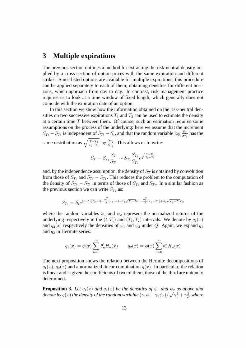
The previous section outlines a method for extracting the risk-neutral density im-plied by a cross-section of option prices with the same expiration and differentstrikes. Since listed options are available for multiple expirations, this procedurecan be applied separately to each of them, obtaining densities for different hori-zons, which approach from day to day. In contrast, risk management practicerequires us to look at a time window of fixed length, which generally does notcoincide with the expiration date of an option.

In this section we show how the information obtained on the risk-neutral den-sities on two successive expirationsT1 andT2 can be used to estimate the densityat a certain timeT between them. Of course, such an estimation requires someassumptions on the process of the underlying: here we assume that the incrementST2 −ST1 is independent ofST1 −St, and that the random variablelog ST

ST1hasthe

same distribution as√

T−T1

T2−T1log

ST2

ST1. This allows us to write:

ST = ST1

ST

ST1

∼ ST1

ST2

ST1

e

√T−T1T2−T1

and,by the independence assumption, the density ofST is obtained by convolutionfrom those ofST1 andST2 − ST1. This reduces the problem to the computation ofthe density ofST2 − ST1 in terms of those ofST1 andST2. In a similar fashion asthe previous section we can writeST2 as:

ST2 = Ste(r−δ)(T2−t)−σ2

12

(T1−t)+σ1√

T1−tψ1−σ222

(T2−T1)+σ2√

T2−T1ψ2

wherethe random variablesψ1 andψ2 represent the normalized returns of theunderlying respectively in the(t, T1) and(T1, T2) intervals. We denote byq1(x)andq2(x) respectively the densities ofψ1 andψ2 underQ. Again, we expandq1

andq2 in Hermite series:

q1(x) = φ(x)∞∑

n=0

θ1nHn(x) q2(x) = φ(x)

∞∑n=0

θ2nHn(x)

The next proposition shows the relation between the Hermite decompositions ofq1(x), q2(x) and a normalized linear combinationq(x). In particular, the relationis linear and is given the coefficients of two of them, those of the third are uniquelydetermined.

Proposition 3. Let q1(x) and q2(x) be the densities ofψ1 and ψ2 as above anddenote byq(x) the density of the random variable(γ1ψ1+γ2ψ2)/

√γ2

1 + γ22 , where

13

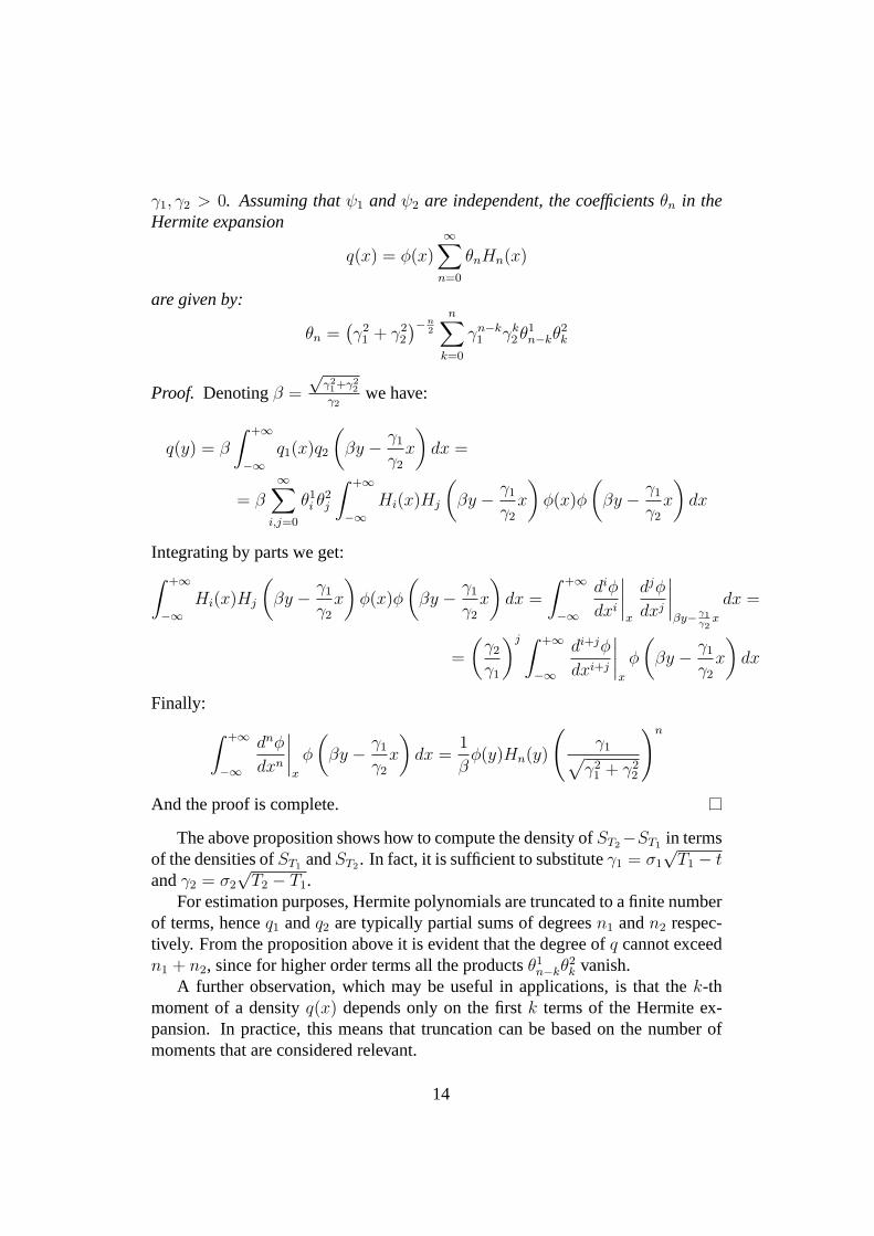
γ1, γ2 > 0. Assuming thatψ1 andψ2 are independent, the coefficientsθn in theHermite expansion

q(x) = φ(x)∞∑

n=0

θnHn(x)

are given by:

θn =(γ2

1 + γ22

)−n2

n∑

k=0

γn−k1 γk

2θ1n−kθ

2k

Proof. Denotingβ =

√γ21+γ2

2

γ2wehave:

q(y) = β

∫ +∞

−∞q1(x)q2

(βy − γ1

γ2

x

)dx =

= β

∞∑i,j=0

θ1i θ

2j

∫ +∞

−∞Hi(x)Hj

(βy − γ1

γ2

x

)φ(x)φ

(βy − γ1

γ2

x

)dx

Integrating by parts we get:∫ +∞

−∞Hi(x)Hj

(βy − γ1

γ2

x

)φ(x)φ

(βy − γ1

γ2

x

)dx =

∫ +∞

−∞

diφ

dxi

∣∣∣∣x

djφ

dxj

∣∣∣∣βy− γ1

γ2x

dx =

=

(γ2

γ1

)j ∫ +∞

−∞

di+jφ

dxi+j

∣∣∣∣x

φ

(βy − γ1

γ2

x

)dx

Finally:

∫ +∞

−∞

dnφ

dxn

∣∣∣∣x

φ

(βy − γ1

γ2

x

)dx =

1

βφ(y)Hn(y)

(γ1√

γ21 + γ2

2

)n

And the proof is complete.

Theabove proposition shows how to compute the density ofST2−ST1 in termsof the densities ofST1 andST2. In fact, it is sufficient to substituteγ1 = σ1

√T1 − t

andγ2 = σ2

√T2 − T1.

For estimation purposes, Hermite polynomials are truncated to a finite numberof terms, henceq1 andq2 are typically partial sums of degreesn1 andn2 respec-tively. From the proposition above it is evident that the degree ofq cannot exceedn1 + n2, since for higher order terms all the productsθ1

n−kθ2k vanish.

A further observation, which may be useful in applications, is that thek-thmoment of a densityq(x) depends only on the firstk terms of the Hermite ex-pansion. In practice, this means that truncation can be based on the number ofmoments that are considered relevant.

14

4 Application to the Italian derivatives market

4.1 Data

We now turn to the estimation of the model to market data. Our dataset consistsof prices and volumes of all transactions on listed options and futures contractson the MIB30 index during the year 1998. These options are traded on the IDEM(Italian derivatives market), a section of the Italian Exchange. For the interestrates, we used the three-month LIBOR on the Italian lira.

Before we discuss empirical issues let us spend a few words on the institutionalfeatures of the market: the MIB30 is a capitalization-weighted index based on afixed basket of the 30 most liquid and highly capitalized common stocks on theItalian Exchange. Since options and futures are traded simultaneously on the sameexchange, there is no time lag between the reporting of option and underlyingprices, unlike in the S&P 500 options market.

Options with expiration in the quarterly cycle of March, June, September andDecember are listed at any time. In addition, the expirations corresponding to thetwo nearest months outside the cycle are made available. In practice, there aresufficient liquid contracts only for the two nearest months, therefore our analysisis constrained to this time horizon. Liquidity tends to decrease near expirationdates as trading shifts from one contract to the next.

4.2 Methodology

Estimation of the risk-neutral density requires the simultaneous observation of across section of options with the same expiration but different strike. In a veryliquid market this is achieved considering the last quote on each contract beforea fixed time of the day. This procedure is not feasible with our dataset, whichdoes not include quotes; even if applicable it would not exploit all the informationembedded in transaction prices, as many options (usually those in-the-money) arethinly traded and bid-ask spreads are very wide.

For each trading day we record the last transaction before noon for each optioncontract as well as the underlying value at the time of each recorded transaction.This ensures that illiquid contracts, which may be traded few times in an hour, arenot associated with the value of the underlying at noon, which may be significantlydifferent from the time of the last transaction.

A critical point is usually the measurement of the underlying value as manyauthors have pointed out that it is often unreliable, either due to a time lag inreporting or to the unobservability of dividends or both. As mentioned before, thefirst issue does not arise in our case, while the latter remains.

A possible solution is suggested by Aıt-Sahalia and Lo, observing that option

15

pricesdepend on the underlying priceST and the dividend yieldδ only throughthe forward price

FT = Ste(r−δ)τ

which can be estimated using the model-independent call-put parity:

Ct(K)− Pt(K) = e−rτ (FT −K)

Attempts to apply this idea to our dataset gave disappointing results as asyn-chronous transactions on calls and puts substantially compromise accuracy. Infact, the estimated underlying price varies widely even in short periods of timeowing to the relative illiquidity of the option market.

However,FT can be estimated from the future price, which is also part of ourdataset and is reported synchronously with option prices. When the expiration ofthe future contract coincides with that of the option, the estimation error is reducedto the difference between the future and the forward prices and to the uncertaintyin expected dividends. As the two expirations may differ for two months at most(since future contracts follow the quarterly cycle), the forward price is obtained bydiscounting the future (we use the three-month LIBOR) but expected dividends inthe expiration lag cannot be eliminated and add up to the estimation error.

Summing up, for each trading day we observe the cross sections of those op-tions with the two nearest expiration months. For each expiration, we have acertain number of strikes (typically from 10 to 20) for which a call or a put option,or both, are available. We keep the contract with higher trading volume, whichgenerally coincides with the one out-of-the money (i.e. calls for high strikes andputs for low strikes).

Denoting byK the set of strikes, for eachK ∈ K we have an option pricePK , the corresponding underlying valueSK , and a dummy variableFK , which isequal to0 for a call option and to1 for a put option. With this notation we canwrite the theoretical priceΠK of a call or put option in the single formula:

ΠK = C(SK , K, r, τ, σ, θ)− FK(e−δτSK − e−rτK)

which is more convenient for estimation purposes than a conditional statement.Then we specify the model as:

PK = ΠK + εK

where{εK}K∈K are IID random variables. The parametersσ andθ can then beestimated by the least-squares method:

χ2(σ, θ) =∑K∈K

(PK − ΠK(FK , SK , K, r, τ, σ, θ))2

(σ, θ) = argminθ,σ

χ2(σ, θ)

16

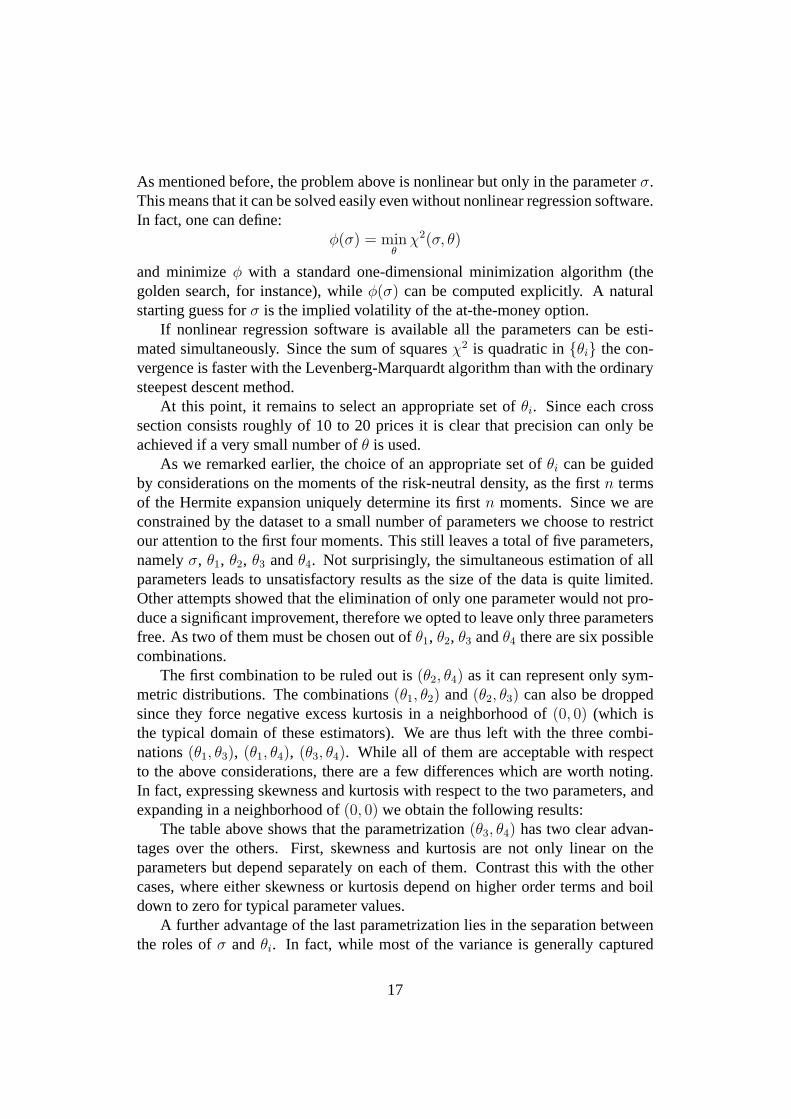
As mentioned before, the problem above is nonlinear but only in the parameterσ.This means that it can be solved easily even without nonlinear regression software.In fact, one can define:

φ(σ) = minθ

χ2(σ, θ)

and minimizeφ with a standard one-dimensional minimization algorithm (thegolden search, for instance), whileφ(σ) can be computed explicitly. A naturalstarting guess forσ is the implied volatility of the at-the-money option.

If nonlinear regression software is available all the parameters can be esti-mated simultaneously. Since the sum of squaresχ2 is quadratic in{θi} the con-vergence is faster with the Levenberg-Marquardt algorithm than with the ordinarysteepest descent method.

At this point, it remains to select an appropriate set ofθi. Since each crosssection consists roughly of 10 to 20 prices it is clear that precision can only beachieved if a very small number ofθ is used.

As we remarked earlier, the choice of an appropriate set ofθi can be guidedby considerations on the moments of the risk-neutral density, as the firstn termsof the Hermite expansion uniquely determine its firstn moments. Since we areconstrained by the dataset to a small number of parameters we choose to restrictour attention to the first four moments. This still leaves a total of five parameters,namelyσ, θ1, θ2, θ3 andθ4. Not surprisingly, the simultaneous estimation of allparameters leads to unsatisfactory results as the size of the data is quite limited.Other attempts showed that the elimination of only one parameter would not pro-duce a significant improvement, therefore we opted to leave only three parametersfree. As two of them must be chosen out ofθ1, θ2, θ3 andθ4 there are six possiblecombinations.

The first combination to be ruled out is(θ2, θ4) as it can represent only sym-metric distributions. The combinations(θ1, θ2) and(θ2, θ3) can also be droppedsince they force negative excess kurtosis in a neighborhood of(0, 0) (which isthe typical domain of these estimators). We are thus left with the three combi-nations(θ1, θ3), (θ1, θ4), (θ3, θ4). While all of them are acceptable with respectto the above considerations, there are a few differences which are worth noting.In fact, expressing skewness and kurtosis with respect to the two parameters, andexpanding in a neighborhood of(0, 0) we obtain the following results:

The table above shows that the parametrization(θ3, θ4) has two clear advan-tages over the others. First, skewness and kurtosis are not only linear on theparameters but depend separately on each of them. Contrast this with the othercases, where either skewness or kurtosis depend on higher order terms and boildown to zero for typical parameter values.

A further advantage of the last parametrization lies in the separation betweenthe roles ofσ andθi. In fact, while most of the variance is generally captured

17

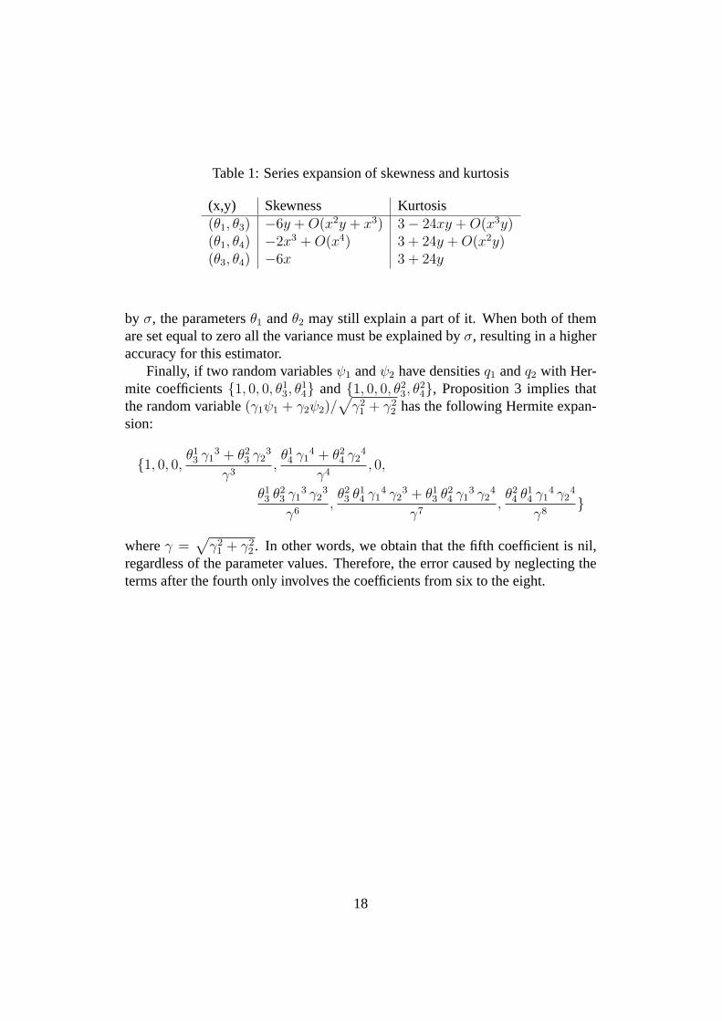
Table 1: Series expansion of skewness and kurtosis

(x,y) Skewness Kurtosis(θ1, θ3) −6y + O(x2y + x3) 3− 24xy + O(x3y)(θ1, θ4) −2x3 + O(x4) 3 + 24y + O(x2y)(θ3, θ4) −6x 3 + 24y

by σ, the parametersθ1 andθ2 may still explain a part of it. When both of themare set equal to zero all the variance must be explained byσ, resulting in a higheraccuracy for this estimator.

Finally, if two random variablesψ1 andψ2 have densitiesq1 andq2 with Her-mite coefficients{1, 0, 0, θ1

3, θ14} and{1, 0, 0, θ2

3, θ24}, Proposition 3 implies that

the random variable(γ1ψ1 + γ2ψ2)/√

γ21 + γ2

2 hasthe following Hermite expan-sion:

{1, 0, 0, θ13 γ1

3 + θ23 γ2

3

γ3,θ14 γ1

4 + θ24 γ2

4

γ4, 0,

θ13 θ2

3 γ13 γ2

3

γ6,θ23 θ1

4 γ14 γ2

3 + θ13 θ2

4 γ13 γ2

4

γ7,θ24 θ1

4 γ14 γ2

4

γ8}

whereγ =√

γ21 + γ2

2 . In other words, we obtain that the fifth coefficient is nil,regardless of the parameter values. Therefore, the error caused by neglecting theterms after the fourth only involves the coefficients from six to the eight.

18

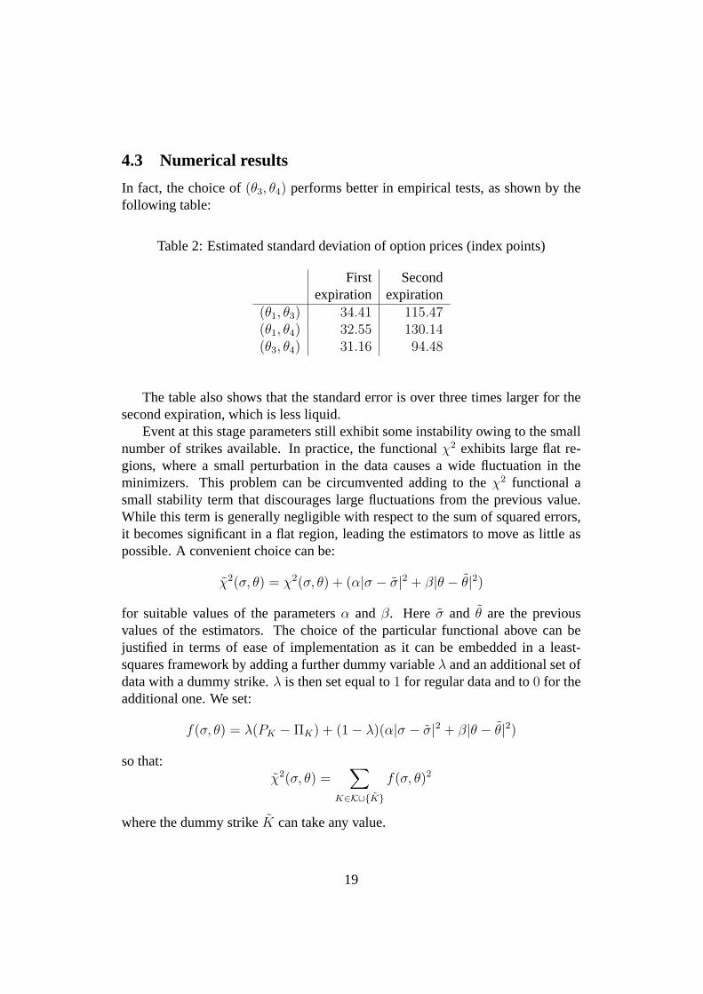
4.3 Numerical results

In fact, the choice of(θ3, θ4) performs better in empirical tests, as shown by thefollowing table:

Table 2: Estimated standard deviation of option prices (index points)

First Secondexpiration expiration

(θ1, θ3) 34.41 115.47(θ1, θ4) 32.55 130.14(θ3, θ4) 31.16 94.48

Thetable also shows that the standard error is over three times larger for thesecond expiration, which is less liquid.

Event at this stage parameters still exhibit some instability owing to the smallnumber of strikes available. In practice, the functionalχ2 exhibits large flat re-gions, where a small perturbation in the data causes a wide fluctuation in theminimizers. This problem can be circumvented adding to theχ2 functional asmall stability term that discourages large fluctuations from the previous value.While this term is generally negligible with respect to the sum of squared errors,it becomes significant in a flat region, leading the estimators to move as little aspossible. A convenient choice can be:

χ2(σ, θ) = χ2(σ, θ) + (α|σ − σ|2 + β|θ − θ|2)

for suitable values of the parametersα and β. Here σ and θ are the previousvalues of the estimators. The choice of the particular functional above can bejustified in terms of ease of implementation as it can be embedded in a least-squares framework by adding a further dummy variableλ and an additional set ofdata with a dummy strike.λ is then set equal to1 for regular data and to0 for theadditional one. We set:

f(σ, θ) = λ(PK − ΠK) + (1− λ)(α|σ − σ|2 + β|θ − θ|2)

so that:χ2(σ, θ) =

∑

K∈K∪{K}f(σ, θ)2

where the dummy strikeK can take any value.

19

Figures1 and 2 show the values of volatility (σ), skewness and kurtosis for thefirst two expirations, estimated with or without the smoothing term in the func-tional: α andβ were both set equal to10. While the addition of the penalizationterm greatly reduces the variance of the estimators, virtually eliminating outliers,in principle it may create a bias. Calculating the differences between the two esti-mators (with or without smoothing) and discarding those values lying outside thecentered95% confidence interval, it turns out that the average biases on volatility,skewness and kurtosis are respectively−1.2%, −71.0% and4.8% of the param-eter averages. In other words, the bias is not serious for volatility and excesskurtosis, while it is significant for skewness.

Figure 3 shows the estimates for a moving horizon of one-month, obtainedusing the procedure in section 3 from the estimates on the first two expirations.In the last set we have the graphs of the parameter estimates versus the index.In the sample period there were two major events affecting the Italian market:the admission to the core group of countries participating to the EMU and theglobal crisis of world markets following the default of Russia. The first eventcaused a strong rally in the Italian index in anticipation of the admission to theEMU, followed by a sharp drop during April. In this case, the option marketcorrectly anticipated the chance of large movements with both implied volatilityand kurtosis rising from mid-March and with skewness decreasing over the sameperiod. On the contrary, the Russian crisis, which caused a much larger drop in theindex, was not anticipated at all by market participants as volatility began to riseonly at the end of August, kurtosis continued to shrink until the end of October,and skewness even rose throughout the crisis.

20

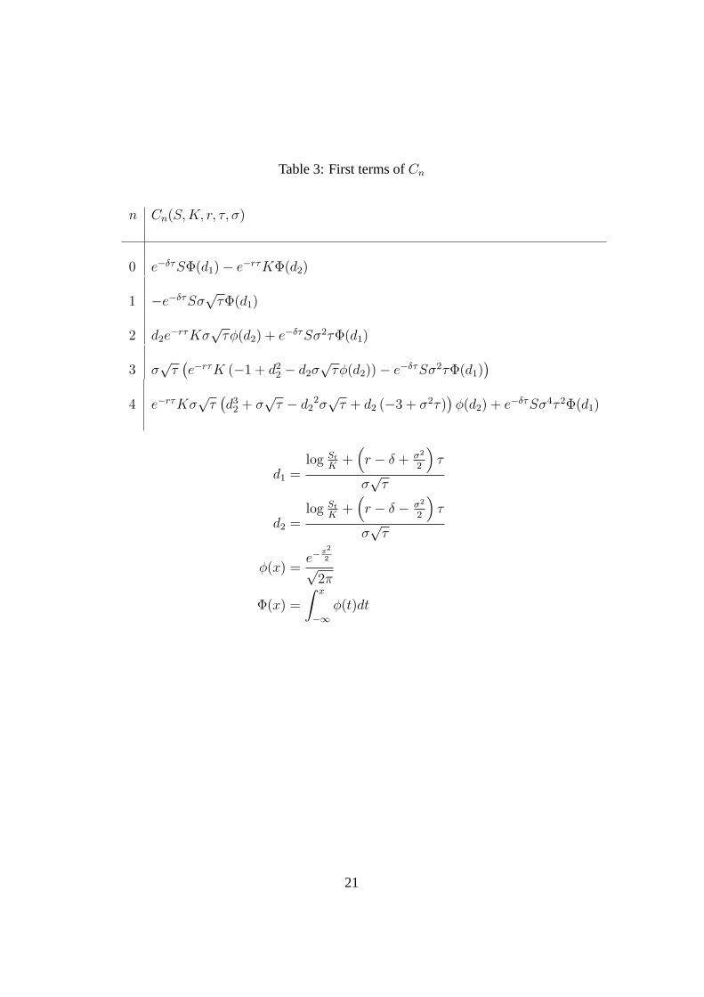
Table 3: First terms ofCn

n Cn(S, K, r, τ, σ)

0 e−δτSΦ(d1)− e−rτKΦ(d2)

1 −e−δτSσ√

τΦ(d1)

2 d2e−rτKσ

√τφ(d2) + e−δτSσ2τΦ(d1)

3 σ√

τ(e−rτK (−1 + d2

2 − d2σ√

τφ(d2))− e−δτSσ2τΦ(d1))

4 e−rτKσ√

τ(d3

2 + σ√

τ − d22σ√

τ + d2 (−3 + σ2τ))φ(d2) + e−δτSσ4τ 2Φ(d1)

d1 =log St

K+

(r − δ + σ2

2

)τ

σ√

τ

d2 =log St

K+

(r − δ − σ2

2

)τ

σ√

τ

φ(x) =e−

x2

2√2π

Φ(x) =

∫ x

−∞φ(t)dt

21

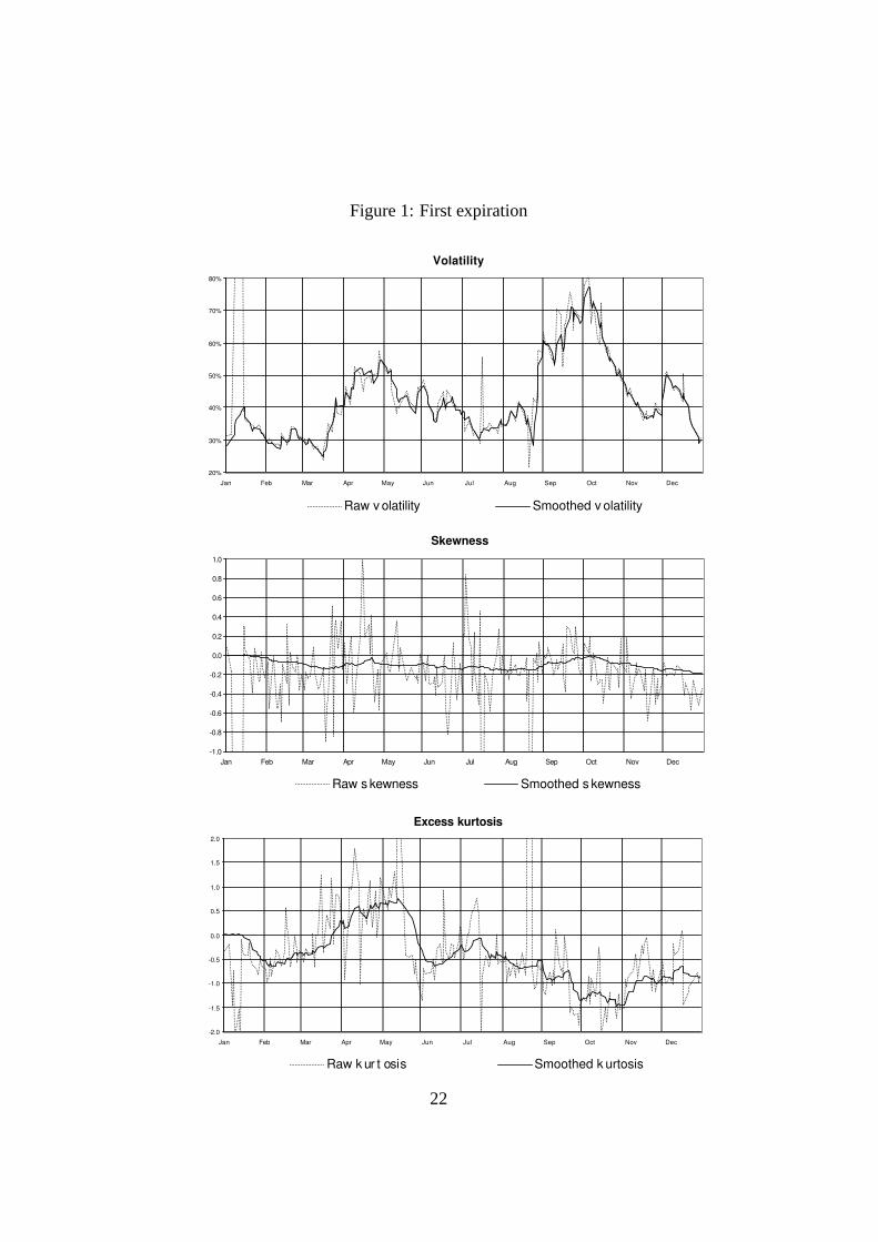
Figure1: First expiration

Volatility

20%

30%

40%

50%

60%

70%

80%

Jan Feb Mar Apr May Jun Jul Aug Sep Oct Nov Dec

Raw v olatility Smoothed v olatility

Skewness

-1.0

-0.8

-0.6

-0.4

-0.2

0.0

0.2

0.4

0.6

0.8

1.0

Jan Feb Mar Apr May Jun Jul Aug Sep Oct Nov Dec

Raw s kewness Smoothed s kewness

Excess kurtosis

-2.0

-1.5

-1.0

-0.5

0.0

0.5

1.0

1.5

2.0

Jan Feb Mar Apr May Jun Jul Aug Sep Oct Nov Dec

Raw k ur t osis Smoothed k urtosis

22

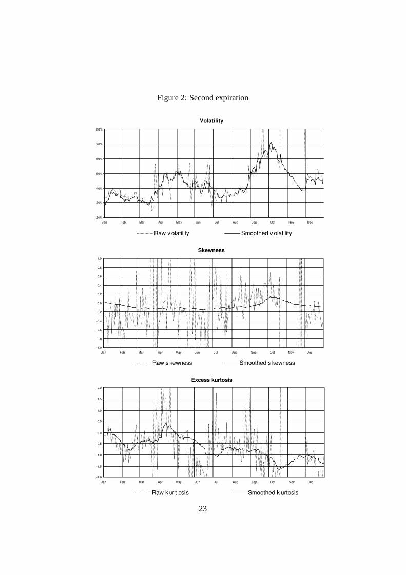
Figure2: Second expiration

Volatility

20%

30%

40%

50%

60%

70%

80%

Jan Feb Mar Apr May Jun Jul Aug Sep Oct Nov Dec

Raw v olatility Smoothed v olatility

Skewness

-1.0

-0.8

-0.6

-0.4

-0.2

0.0

0.2

0.4

0.6

0.8

1.0

Jan Feb Mar Apr May Jun Jul Aug Sep Oct Nov Dec

Raw s kewness Smoothed s kewness

Excess kurtosis

-2.0

-1.5

-1.0

-0.5

0.0

0.5

1.0

1.5

2.0

Jan Feb Mar Apr May Jun Jul Aug Sep Oct Nov Dec

Raw k ur t osis Smoothed k urtosis

23

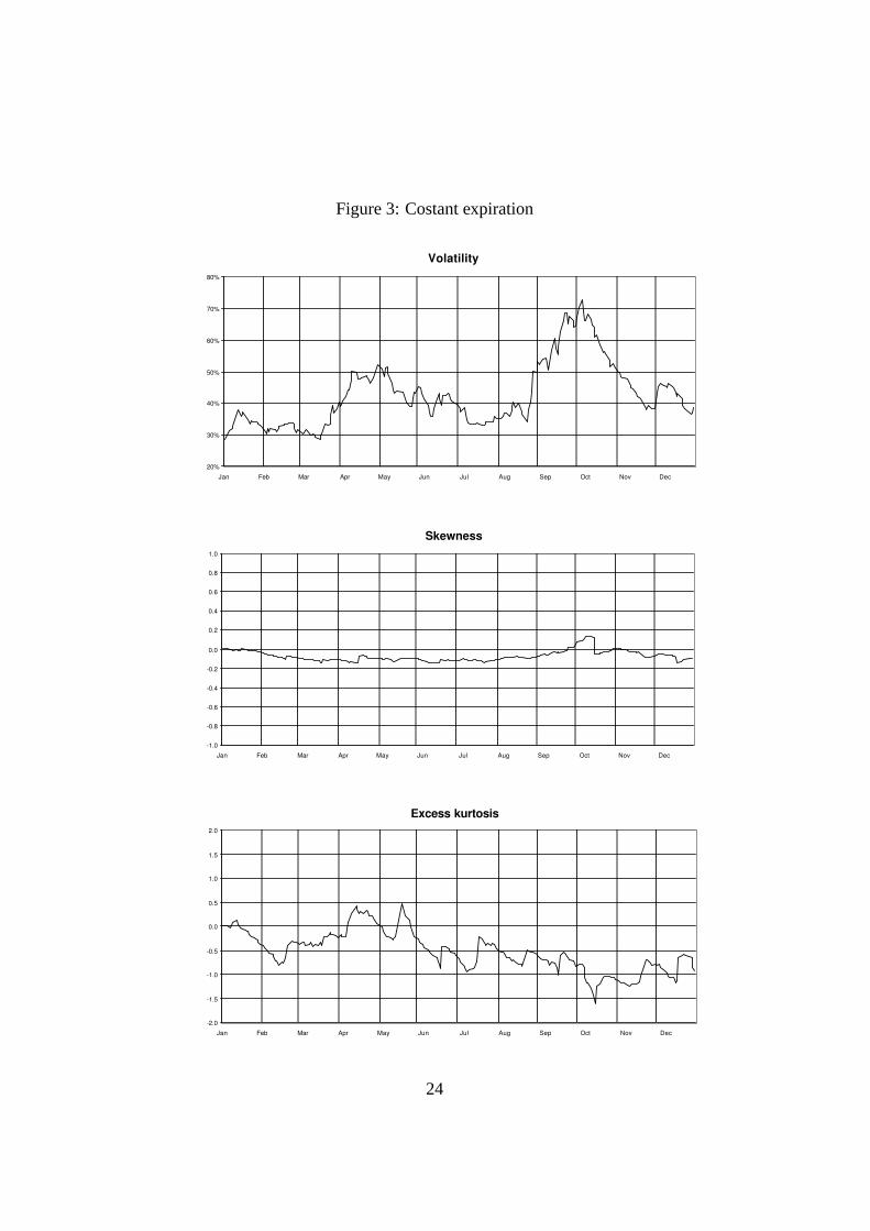
Figure3: Costant expiration

Volatility

20%

30%

40%

50%

60%

70%

80%

Jan Feb Mar Apr May Jun Jul Aug Sep Oct Nov Dec

Skewness

-1.0

-0.8

-0.6

-0.4

-0.2

0.0

0.2

0.4

0.6

0.8

1.0

Jan Feb Mar Apr May Jun Jul Aug Sep Oct Nov Dec

Excess kurtosis

-2.0

-1.5

-1.0

-0.5

0.0

0.5

1.0

1.5

2.0

Jan Feb Mar Apr May Jun Jul Aug Sep Oct Nov Dec

24

References

[1] Yacine Aıt Sahalia and Andrew Lo. Nonparametric estimation of state-pricedensities implicit in financial asset prices.Journal of Finance, 53:299–547,July 1998.

[2] Robert Engle and Joshua Rosenberg. Empirical pricing kernels. Stern Schoolof Business Working Paper, July 2000.

[3] S. Heston. A closed-form solution for option with stochastic volatility withapplications to bond and currency options.Review of Financial Studies,6:327–343, 1993.

[4] Dilip B. Madan and Frank Milne. Contingent claims valued and hedged bypricing and investing in a basis.Math. Finance, 4(3):223–245, 1994.

[5] Mark Rubinstein. Implied binomial trees.Journal of Finance, July 1994.

[6] David Shimko. Bounds of probability.Risk, 6:33–37, 1993.

[7] E. M. Stein and J. C. Stein. Stock price distributions with stochastic volatility:an analytic approach.Review of Financial Studies, 4:727–752, 1991.

RECENTLY PUBLISHED “TEMI” (*)

N. 481 – Bank competition and firm creation, by E. BONACCORSI DI PATTI and G. DELL’ARICCIA (June 2003).

N. 482 – La distribuzione del reddito e della ricchezza nelle regioni italiane, by L. CANNARI and G. D’ALESSIO (June 2003).

N. 483 – Risk aversion, wealth and background risk, by L. GUISO and M. PAIELLA (September 2003).

N. 484 – What is this thing called confidence? A comparative analysis of consumer indices in eight major countries, by R. GOLINELLI and G. PARIGI (September 2003).

N. 485 – L’utilizzo degli indicatori compositi nell’analisi congiunturale territoriale: un’applicazione all’economia del Veneto, by P. CHIADES, M. GALLO andA. VENTURINI (September 2003).

N. 486 – Bank capital and lending behaviour: empirical evidence for Italy, byL. GAMBACORTA and P. E. MISTRULLI (September 2003).

N. 487 – A polarization of polarization? The distribution of inequality 1970-1996, by C. BIANCOTTI (March 2004).

N. 488 – Pitfalls of monetary policy under incomplete information: imprecise indicators and real indeterminacy, by E. GAIOTTI (March 2004).

N. 489 – Information technology and productivity changes in the banking industry, by L. CASOLARO and G. GOBBI (March 2004).

N. 490 – La bilancia dei pagamenti di parte corrente Nord-Sud (1998-2000), by L. CANNARI and S. CHIRI (March 2004).

N. 491 – Investire in Italia? Risultati di una recente indagine empirica, by M. COMMITTERI (March 2004).

N. 492 – Centralization of wage bargaining and the unemployment rate: revisiting the hump-shape hypothesis, by L. FORNI (June 2004).

N. 493 – Endogenous monetary policy with unobserved potential output, by A. CUKIERMAN and F. LIPPI (June 2004).

N. 494 – Il credito commerciale: problemi e teorie, by M. OMICCIOLI (June 2004).

N. 495 – Condizioni di credito commerciale e differenziazione della clientela,byL. CANNARI, S. CHIRI aND M. OMICCIOLI (June 2004).

N. 496 – Il debito commerciale in Italia: quanto contano le motivazioni finanziarie?, byP. FINALDI RUSSO and L. LEVA (June 2004).

N. 497 – Funzionamento della giustizia civile e struttura finanziaria delle imprese: il ruolo del credito commerciale, by A. CARMIGNANI (June 2004).

N. 498 – Does trade credit substitute for bank credit?, by G. DE BLASIO (June 2004).

N. 499 – Monetary policy and the transition to rational expectations, by G. FERRERO (June 2004).

N. 500 – Turning-point indicators from business surveys: real-time detection for the euro area and its major member countries, by A. BAFFIGI and A. BASSANETTI (June 2004).

N. 501 – La ricchezza delle famiglie italiane e americane, by I. FAIELLA and A. NERI (June 2004).

N. 502 – Optimal duplication of effort in advocacy systems, by G. PALUMBO (June 2004).

N. 503 – Il pilastro privato del sistema previdenziale. Il caso del Regno Unito, byF. SPADAFORA (June 2004).

N. 504 – Firm size distribution and employment protection legislation in Italy, byF. SCHIVARDI and R. TORRINI (June 2004).

N. 505 – Social mobility and endogenous cycles in redistribution, by F. ZOLLINO (July 2004).

N. 506 – Estimating expectations of shocks using option prices, by A. DI CESARE (July 2004).

(*) Requests for copies should be sent to:Banca d’Italia – Servizio Studi – Divisione Biblioteca e pubblicazioni – Via Nazionale, 91 – 00184 Rome(fax 0039 06 47922059). They area available on the Internet www.bancaditalia.it.

"TEMI" LATER PUBLISHED ELSEWHERE

1999

L. GUISO and G. PARIGI, Investment and demand uncertainty, Quarterly Journal of Economics, Vol. 114(1), pp. 185-228, TD No. 289 (November 1996).

A. F. POZZOLO, Gli effetti della liberalizzazione valutaria sulle transazioni finanziarie dell’Italia conl’estero, Rivista di Politica Economica, Vol. 89 (3), pp. 45-76, TD No. 296 (February 1997).

A. CUKIERMAN and F. LIPPI, Central bank independence, centralization of wage bargaining, inflation andunemployment: theory and evidence, European Economic Review, Vol. 43 (7), pp. 1395-1434, TDNo. 332 (April 1998).

P. CASELLI and R. RINALDI, La politica fiscale nei paesi dell’Unione europea negli anni novanta, Studi enote di economia, (1), pp. 71-109, TD No. 334 (July 1998).

A. BRANDOLINI, The distribution of personal income in post-war Italy: Source description, data quality,and the time pattern of income inequality, Giornale degli economisti e Annali di economia, Vol. 58(2), pp. 183-239, TD No. 350 (April 1999).

L. GUISO, A. K. KASHYAP, F. PANETTA and D. TERLIZZESE, Will a common European monetary policyhave asymmetric effects?, Economic Perspectives, Federal Reserve Bank of Chicago, Vol. 23 (4),pp. 56-75, TD No. 384 (October 2000).

2000

P. ANGELINI, Are banks risk-averse? Timing of the operations in the interbank market, Journal of Money,Credit and Banking, Vol. 32 (1), pp. 54-73, TD No. 266 (April 1996).

F. DRUDI and R: GIORDANO, Default Risk and optimal debt management, Journal of Banking and Finance,Vol. 24 (6), pp. 861-892, TD No. 278 (September 1996).

F. DRUDI and R. GIORDANO, Wage indexation, employment and inflation, Scandinavian Journal ofEconomics, Vol. 102 (4), pp. 645-668, TD No. 292 (December 1996).

F. DRUDI and A. PRATI, Signaling fiscal regime sustainability, European Economic Review, Vol. 44 (10),pp. 1897-1930, TD No. 335 (September 1998).

F. FORNARI and R. VIOLI, The probability density function of interest rates implied in the price of options,in: R. Violi, (ed.) , Mercati dei derivati, controllo monetario e stabilità finanziaria, Il Mulino,Bologna, TD No. 339 (October 1998).

D. J. MARCHETTI and G. PARIGI, Energy consumption, survey data and the prediction of industrialproduction in Italy, Journal of Forecasting, Vol. 19 (5), pp. 419-440, TD No. 342 (December1998).

A. BAFFIGI, M. PAGNINI and F. QUINTILIANI, Localismo bancario e distretti industriali: assetto dei mercatidel credito e finanziamento degli investimenti, in: L.F. Signorini (ed.), Lo sviluppo locale:un'indagine della Banca d'Italia sui distretti industriali, Donzelli, TD No. 347 (March 1999).

A. SCALIA and V. VACCA, Does market transparency matter? A case study, in: Market Liquidity: ResearchFindings and Selected Policy Implications, Basel, Bank for International Settlements, TD No. 359(October 1999).

F. SCHIVARDI, Rigidità nel mercato del lavoro, disoccupazione e crescita, Giornale degli economisti eAnnali di economia, Vol. 59 (1), pp. 117-143, TD No. 364 (December 1999).

G. BODO, R. GOLINELLI and G. PARIGI, Forecasting industrial production in the euro area, EmpiricalEconomics, Vol. 25 (4), pp. 541-561, TD No. 370 (March 2000).

F. ALTISSIMO, D. J. MARCHETTI and G. P. ONETO, The Italian business cycle: Coincident and leadingindicators and some stylized facts, Giornale degli economisti e Annali di economia, Vol. 60 (2), pp.147-220, TD No. 377 (October 2000).

C. MICHELACCI and P. ZAFFARONI, (Fractional) Beta convergence, Journal of Monetary Economics, Vol.45, pp. 129-153, TD No. 383 (October 2000).

R. DE BONIS and A. FERRANDO, The Italian banking structure in the nineties: testing the multimarketcontact hypothesis, Economic Notes, Vol. 29 (2), pp. 215-241, TD No. 387 (October 2000).

2001

M. CARUSO, Stock prices and money velocity: A multi-country analysis, Empirical Economics, Vol. 26(4), pp. 651-72, TD No. 264 (February 1996).

P. CIPOLLONE and D. J. MARCHETTI, Bottlenecks and limits to growth: A multisectoral analysis of Italianindustry, Journal of Policy Modeling, Vol. 23 (6), pp. 601-620, TD No. 314 (August 1997).

P. CASELLI, Fiscal consolidations under fixed exchange rates, European Economic Review, Vol. 45 (3),pp. 425-450, TD No. 336 (October 1998).

F. ALTISSIMO and G. L. VIOLANTE, Nonlinear VAR: Some theory and an application to US GNP andunemployment, Journal of Applied Econometrics, Vol. 16 (4), pp. 461-486, TD No. 338 (October1998).

F. NUCCI and A. F. POZZOLO, Investment and the exchange rate, European Economic Review, Vol. 45 (2),pp. 259-283, TD No. 344 (December 1998).

L. GAMBACORTA, On the institutional design of the European monetary union: Conservatism, stabilitypact and economic shocks, Economic Notes, Vol. 30 (1), pp. 109-143, TD No. 356 (June 1999).

P. FINALDI RUSSO and P. ROSSI, Credit costraints in italian industrial districts, Applied Economics, Vol.33 (11), pp. 1469-1477, TD No. 360 (December 1999).

A. CUKIERMAN and F. LIPPI, Labor markets and monetary union: A strategic analysis, Economic Journal,Vol. 111 (473), pp. 541-565, TD No. 365 (February 2000).

G. PARIGI and S. SIVIERO, An investment-function-based measure of capacity utilisation, potential outputand utilised capacity in the Bank of Italy’s quarterly model, Economic Modelling, Vol. 18 (4), pp.525-550, TD No. 367 (February 2000).

F. BALASSONE and D. MONACELLI, Emu fiscal rules: Is there a gap?, in: M. Bordignon and D. Da Empoli(eds.), Politica fiscale, flessibilità dei mercati e crescita, Milano, Franco Angeli, TD No. 375 (July2000).

A. B. ATKINSON and A. BRANDOLINI, Promise and pitfalls in the use of “secondary" data-sets: Incomeinequality in OECD countries, Journal of Economic Literature, Vol. 39 (3), pp. 771-799, TD No.379 (October 2000).

D. FOCARELLI and A. F. POZZOLO, The determinants of cross-border bank shareholdings: An analysis withbank-level data from OECD countries, Journal of Banking and Finance, Vol. 25 (12), pp. 2305-2337, TD No. 381 (October 2000).

M. SBRACIA and A. ZAGHINI, Expectations and information in second generation currency crises models,Economic Modelling, Vol. 18 (2), pp. 203-222, TD No. 391 (December 2000).

F. FORNARI and A. MELE, Recovering the probability density function of asset prices using GARCH asdiffusion approximations, Journal of Empirical Finance, Vol. 8 (1), pp. 83-110, TD No. 396(February 2001).

P. CIPOLLONE, La convergenza dei salari manifatturieri in Europa, Politica economica, Vol. 17 (1), pp.97-125, TD No. 398 (February 2001).

E. BONACCORSI DI PATTI and G. GOBBI, The changing structure of local credit markets: Are smallbusinesses special?, Journal of Banking and Finance, Vol. 25 (12), pp. 2209-2237, TD No. 404(June 2001).

G. MESSINA, Decentramento fiscale e perequazione regionale. Efficienza e redistribuzione nel nuovosistema di finanziamento delle regioni a statuto ordinario, Studi economici, Vol. 56 (73), pp. 131-148, TD No. 416 (August 2001).

2002

R. CESARI and F. PANETTA, Style, fees and performance of Italian equity funds, Journal of Banking andFinance, Vol. 26 (1), TD No. 325 (January 1998).

L. GAMBACORTA, Asymmetric bank lending channels and ECB monetary policy, Economic Modelling,Vol. 20 (1), pp. 25-46, TD No. 340 (October 1998).

C. GIANNINI, “Enemy of none but a common friend of all”? An international perspective on the lender-of-last-resort function, Essay in International Finance, Vol. 214, Princeton, N. J., Princeton UniversityPress, TD No. 341 (December 1998).

A. ZAGHINI, Fiscal adjustments and economic performing: A comparative study, Applied Economics, Vol.33 (5), pp. 613-624, TD No. 355 (June 1999).

F. ALTISSIMO, S. SIVIERO and D. TERLIZZESE, How deep are the deep parameters?, Annales d’Economie etde Statistique,.(67/68), pp. 207-226, TD No. 354 (June 1999).

F. FORNARI, C. MONTICELLI, M. PERICOLI and M. TIVEGNA, The impact of news on the exchange rate ofthe lira and long-term interest rates, Economic Modelling, Vol. 19 (4), pp. 611-639, TD No. 358(October 1999).

D. FOCARELLI, F. PANETTA and C. SALLEO, Why do banks merge?, Journal of Money, Credit and Banking,Vol. 34 (4), pp. 1047-1066, TD No. 361 (December 1999).

D. J. MARCHETTI, Markup and the business cycle: Evidence from Italian manufacturing branches, OpenEconomies Review, Vol. 13 (1), pp. 87-103, TD No. 362 (December 1999).

F. BUSETTI, Testing for stochastic trends in series with structural breaks, Journal of Forecasting, Vol. 21(2), pp. 81-105, TD No. 385 (October 2000).

F. LIPPI, Revisiting the Case for a Populist Central Banker, European Economic Review, Vol. 46 (3), pp.601-612, TD No. 386 (October 2000).

F. PANETTA, The stability of the relation between the stock market and macroeconomic forces, EconomicNotes, Vol. 31 (3), TD No. 393 (February 2001).

G. GRANDE and L. VENTURA, Labor income and risky assets under market incompleteness: Evidence fromItalian data, Journal of Banking and Finance, Vol. 26 (2-3), pp. 597-620, TD No. 399 (March2001).

A. BRANDOLINI, P. CIPOLLONE and P. SESTITO, Earnings dispersion, low pay and household poverty inItaly, 1977-1998, in D. Cohen, T. Piketty and G. Saint-Paul (eds.), The Economics of RisingInequalities, pp. 225-264, Oxford, Oxford University Press, TD No. 427 (November 2001).

L. CANNARI and G. D’ALESSIO, La distribuzione del reddito e della ricchezza nelle regioni italiane, RivistaEconomica del Mezzogiorno (Trimestrale della SVIMEZ), Vol. XVI(4), pp. 809-847, Il Mulino,TD No. 482 (June 2003).

2003

F. SCHIVARDI, Reallocation and learning over the business cycle, European Economic Review, , Vol. 47(1), pp. 95-111, TD No. 345 (December 1998).

P. CASELLI, P. PAGANO and F. SCHIVARDI, Uncertainty and slowdown of capital accumulation in Europe,Applied Economics, Vol. 35 (1), pp. 79-89, TD No. 372 (March 2000).

P. PAGANO and G. FERRAGUTO, Endogenous growth with intertemporally dependent preferences,Contribution to Macroeconomics, Vol. 3 (1), pp. 1-38, TD No. 382 (October 2000).

P. PAGANO and F. SCHIVARDI, Firm size distribution and growth, Scandinavian Journal of Economics, Vol.105(2), pp. 255-274, TD No. 394 (February 2001).

M. PERICOLI and M. SBRACIA, A Primer on Financial Contagion, Journal of Economic Surveys, TD No.407 (June 2001).

M. SBRACIA and A. ZAGHINI, The role of the banking system in the international transmission of shocks,World Economy, TD No. 409 (June 2001).

E. GAIOTTI and A. GENERALE, Does monetary policy have asymmetric effects? A look at the investmentdecisions of Italian firms, Giornale degli Economisti e Annali di Economia, Vol. 61 (1), pp. 29-59,TD No. 429 (December 2001).

L. GAMBACORTA, The Italian banking system and monetary policy transmission: evidence from bank leveldata, in: I. Angeloni, A. Kashyap and B. Mojon (eds.), Monetary Policy Transmission in the EuroArea, Cambridge, Cambridge University Press, TD No. 430 (December 2001).

M. EHRMANN, L. GAMBACORTA, J. MARTÍNEZ PAGÉS, P. SEVESTRE and A. WORMS, Financial systems andthe role of banks in monetary policy transmission in the euro area, in: I. Angeloni, A. Kashyap andB. Mojon (eds.), Monetary Policy Transmission in the Euro Area, Cambridge, CambridgeUniversity Press, TD No. 432 (December 2001).

F. SPADAFORA, Financial crises, moral hazard and the speciality of the international market: furtherevidence from the pricing of syndicated bank loans to emerging markets, Emerging MarketsReview, Vol. 4 ( 2), pp. 167-198, TD No. 438 (March 2002).

D. FOCARELLI and F. PANETTA, Are mergers beneficial to consumers? Evidence from the market for bankdeposits, American Economic Review, Vol. 93 (4), pp. 1152-1172, TD No. 448 (July 2002).

E.VIVIANO, Un'analisi critica delle definizioni di disoccupazione e partecipazione in Italia, PoliticaEconomica, Vol. 19 (1), pp. 161-190, TD No. 450 (July 2002).

F. BUSETTI and A. M. ROBERT TAYLOR, Testing against stochastic trend and seasonality in the presence ofunattended breaks and unit roots, Journal of Econometrics, Vol. 117 (1), pp. 21-53, TD No. 470(February 2003).

2004

P. CHIADES and L. GAMBACORTA, The Bernanke and Blinder model in an open economy: The Italian case,German Economic Review, Vol. 5 (1), pp. 1-34, TD No. 388 (December 2000).

M. PAIELLA, Heterogeneity in financial market participation: appraising its implications for the C-CAPM,Review of Finance, Vol. 8, pp. 1-36, TD No. 473 (June 2003).

E. BONACCORSI DI PATTI and G. DELL’ARICCIA, Bank competition and firm creation, Journal of MoneyCredit and Banking, Vol. 36 (2), pp. 225-251, TD No. 481 (June 2003).

R. GOLINELLI and G. PARIGI, Consumer sentiment and economic activity: a cross country comparison,Journal of Business Cycle Measurement and Analysis, Vol. 1 (2), TD No. 484 (September 2003).

FORTHCOMING

A. F. POZZOLO, Research and development regional spillovers, and the localisation of economic activities,The Manchester School, TD No. 331 (March 1998).

F. LIPPI, Strategic monetary policy with non-atomistic wage-setters, Review of Economic Studies, TD No.374 (June 2000).

P. ANGELINI and N. CETORELLI, Bank competition and regulatory reform: The case of the Italian bankingindustry, Journal of Money, Credit and Banking, TD No. 380 (October 2000).

L. DEDOLA AND F. LIPPI, The Monetary Transmission Mechanism: Evidence from the industry Data of FiveOECD Countries, European Economic Review, TD No. 389 (December 2000).

M. BUGAMELLI and P. PAGANO, Barriers to Investment in ICT, Applied Economics, TD No. 420 (October2001).

D. J. MARCHETTI and F. NUCCI, Price Stickiness and the Contractionary Effects of Technology Shocks,European Economic Review, TD No. 392 (February 2001).

G. CORSETTI, M. PERICOLI and M. SBRACIA, Correlation analysis of financial contagion: what one shouldknow before running a test, Journal of International Money and Finance, TD No. 408 (June 2001).

D. FOCARELLI, Bootstrap bias-correction procedure in estimating long-run relationships from dynamic

panels, with an application to money demand in the euro area, Economic Modelling, TD No. 440(March 2002).

A. BAFFIGI, R. GOLINELLI and G. PARIGI, Bridge models to forecast the euro area GDP, InternationalJournal of Forecasting, TD No. 456 (December 2002).

F. CINGANO and F. SCHIVARDI, Identifying the sources of local productivity growth, Journal of theEuropean Economic Association, TD NO. 474 (June 2003).

E. BARUCCI, C. IMPENNA and R. RENÒ, Monetary integration, markets and regulation, Research inBanking and Finance, TD NO. 475 (June 2003).

G. ARDIZZI, Cost efficiency in the retail payment networks:first evidence from the Italian credit cardsystem, Rivista di Politica Economica, TD NO. 480 (June 2003).

L. GAMBACORTA and P. E. Mistrulli, Does bank capital affect lending behavior?, Journal of FinancialIntermediation, TD NO. 486 (September 2003).