Data Visualization with R (I)

Dr. Jieh-Shan George YEHjsyeh@pu.edu.tw

2

Outlines

• Data Visualization with R• Visualizing Different Type of Data– Univariate– Univariate Categorical– Bivariate Categorical– Bivariate Continuous vs Categorical– Bivariate Continuous vs Continuous– Bivariate: Continuous vs Time

3

Data Visualization with R

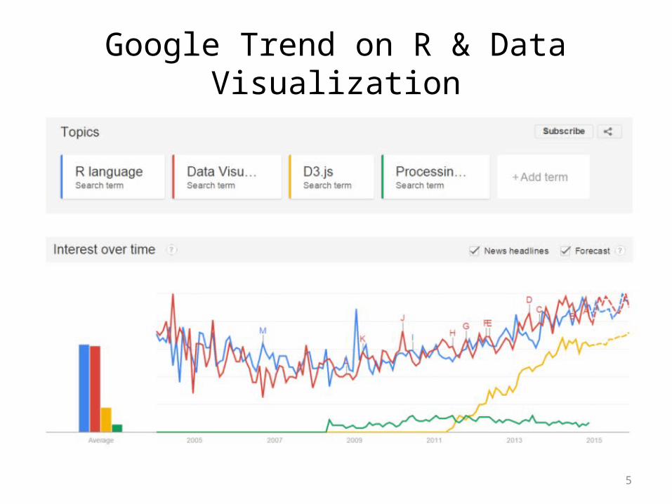
• Both anecdotally, and per Google Trends, R is the language and tool most closely associated with creating data visualizations. – http://www.google.com/trends/explore?hl=en-US#q=

R%20language,%20Data%20Visualization,%20D3.js,%20Processing.js&cmpt=q

4

Google Trend on R & Data Visualization

5

Google Trend on R & Data Visualization

6

UNIVARIATE

7

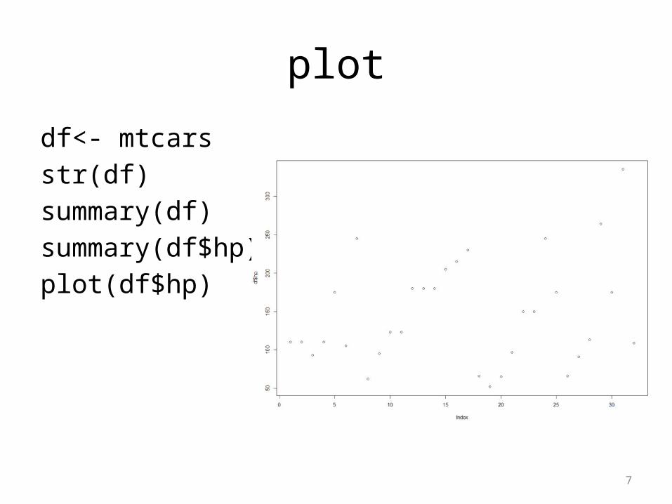
plot

df<- mtcarsstr(df)summary(df)summary(df$hp)plot(df$hp)

8

Univariate: boxplot

• # Boxplot for univariate• boxplot(df$hp,

horizontal=TRUE, notch=TRUE, col="gold")

9

Univariate: robustbase::adjbox

install.packages("robustbase")library(robustbase)robustbase::adjbox(df$hp, horizontal=TRUE, cex=2, lwd=0.5, main="robustbase::adjbox()", notch=TRUE, col="skyblue")

10

Univariate: vioplot::vioplot

install.packages("vioplot")library(vioplot)vioplot::vioplot(df$hp, col="lightgreen", horizontal=TRUE)

11

Univariate: Historgam

##the counts component of the result

hist(df$hp, xlab="Gross horsepower", ylab="Number of cars", labels=TRUE, col="skyblue")

12

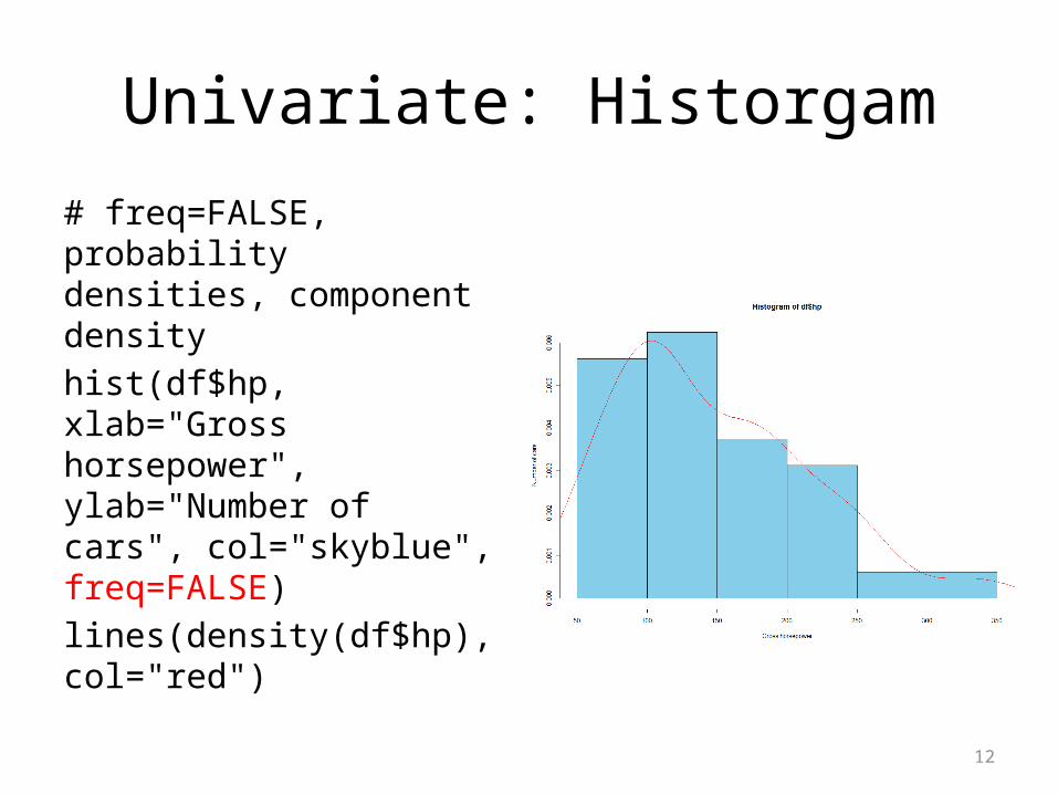
Univariate: Historgam

# freq=FALSE, probability densities, component densityhist(df$hp, xlab="Gross horsepower", ylab="Number of cars", col="skyblue", freq=FALSE)lines(density(df$hp), col="red")

13

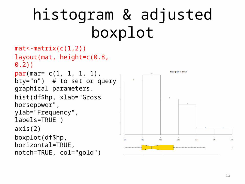
histogram & adjusted boxplot

mat<-matrix(c(1,2))layout(mat, height=c(0.8, 0.2))par(mar= c(1, 1, 1, 1), bty="n") # to set or query graphical parameters.hist(df$hp, xlab="Gross horsepower", ylab="Frequency", labels=TRUE )axis(2)boxplot(df$hp, horizontal=TRUE, notch=TRUE, col="gold")

14

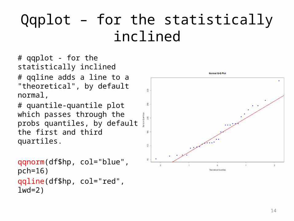
Qqplot – for the statistically inclined

# qqplot - for the statistically inclined # qqline adds a line to a "theoretical", by default normal, # quantile-quantile plot which passes through the probs quantiles, by default the first and third quartiles.

qqnorm(df$hp, col="blue", pch=16)qqline(df$hp, col="red", lwd=2)

15

UNIVARIATE CATEGORICAL

16

Univariate Categorical

#Topics most visited on English Wikipedia on 31 May 2013

Topic <- c("Cult", "Rituparno Ghosh", "Cat anatomy", "Facebook", "Fast & Furious 6", "Liberace", "Game of Thrones", "Jean-Claude Romand", "Game of Thrones (season 3)", "Arrested Development (TV series)")

NoHit <- c(291439, 215843, 102960, 93181, 84014, 73162, 70599, 70144, 69752, 69573)

wiki <- NoHitnames(wiki)<- Topic

17

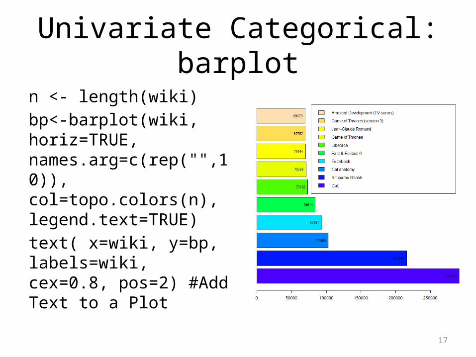
Univariate Categorical: barplot

n <- length(wiki) bp<-barplot(wiki, horiz=TRUE, names.arg=c(rep("",10)), col=topo.colors(n), legend.text=TRUE) text( x=wiki, y=bp, labels=wiki, cex=0.8, pos=2) #Add Text to a Plot

18

Univariate Categorical: pie

# pie pie(wiki, init.angle=90)

19

Univariate Categorical: pie3D

require(plotrix)pie3D(wiki, labels = names(wiki), explode=0.1)

20

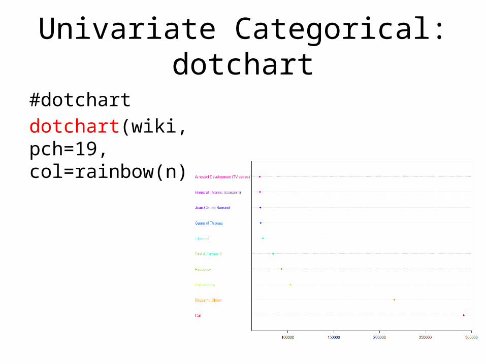
Univariate Categorical: dotchart

#dotchartdotchart(wiki, pch=19, col=rainbow(n))

21

BIVARIATE CATEGORICAL

22

Bivariate Categorical: barpplot

#Stacked bar plot mycols <- c("Brown", "Blue", "Yellow", "Green")barplot( HairEyeColor[,,1], col=mycols) legend( x="topright", legend = attr(HairEyeColor, "dimnames")$Eye, pch=18, col=mycols)

23

Bivariate Categorical: barpplot

barplot( HairEyeColor[,,1], col=mycols, beside=TRUE) legend( x="topright", legend = attr(HairEyeColor, "dimnames")$Eye, pch=18, col=mycols)

24

Bivariate Categorical: mosaicplot

#mosaic gridmosaicplot(HairEyeColor[,,1], col=mycols)

25

BIVARIATE CONTINUOUS VS CATEGORICAL

26

bivariate Continuous vs Categorical: boxplot

mtcars

attach(mtcars)

boxplot(mpg~cyl, data=mtcars, col=c("darkorange","blue","gold"))

27

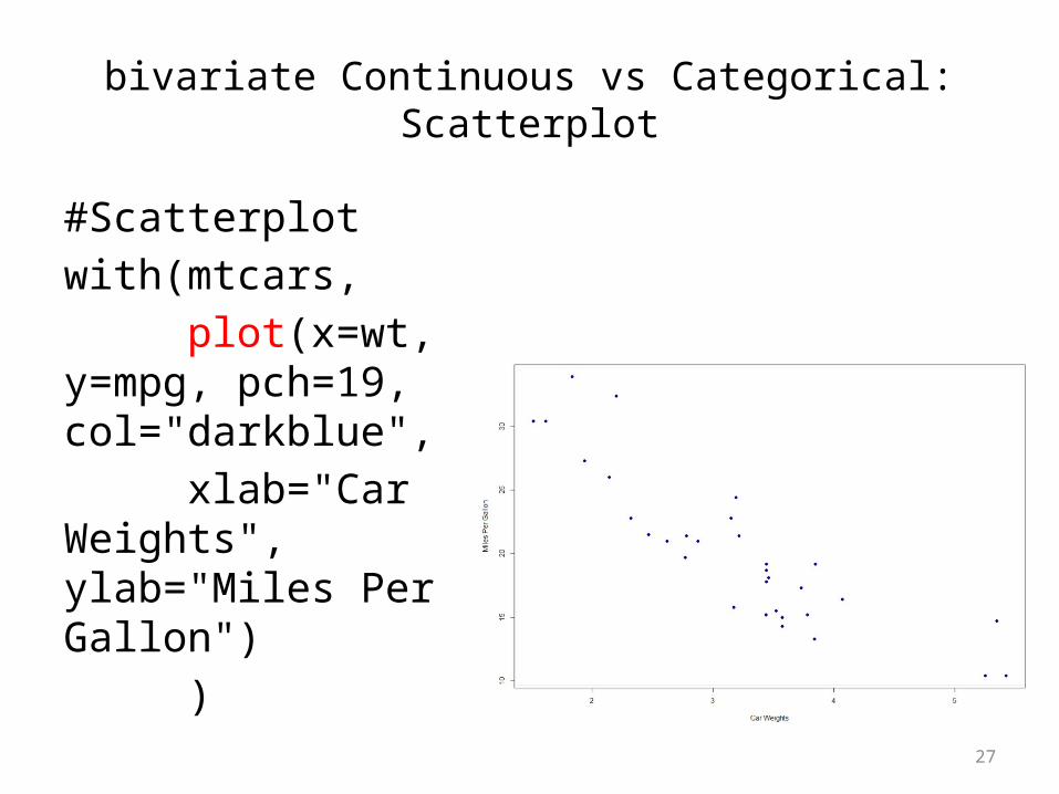
bivariate Continuous vs Categorical:Scatterplot

#Scatterplotwith(mtcars, plot(x=wt, y=mpg, pch=19, col="darkblue", xlab="Car Weights", ylab="Miles Per Gallon") )

28

bivariate Continuous vs Categorical:Scatterplot – fitted lines

#Scatterplot fitted linewith(mtcars, abline(lsfit(x=wt, y=mpg) , col="red"))

with(mtcars, lines(lowess(x=wt, y=mpg), col="green"))

29

car::scatterplot

#car::scatterplotrequire(car)scatterplot(mpg~wt, data=mtcars)

30

Bivariate boxplot - bagplot

#Bivariate boxplot - bagplotinstall.packages(aplpack)require(aplpack)with(mtcars, bagplot(wt, mpg))

31

BIVARIATE CONTINUOUS VS CONTINUOUS

32

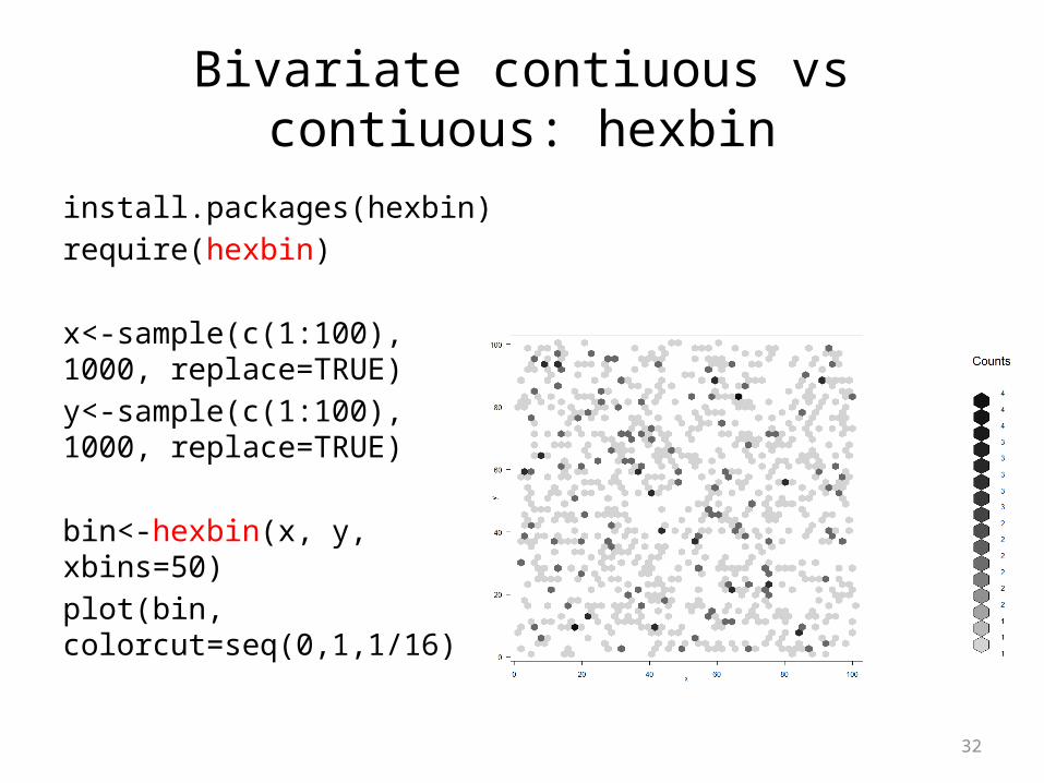
Bivariate contiuous vs contiuous: hexbin

install.packages(hexbin)require(hexbin)

x<-sample(c(1:100), 1000, replace=TRUE)y<-sample(c(1:100), 1000, replace=TRUE)

bin<-hexbin(x, y, xbins=50)plot(bin, colorcut=seq(0,1,1/16))

33

Bivariate contiuous vs contiuous: hexbin

• h <- hexbin(rnorm(10000),rnorm(10000))

• plot(h, colramp= BTY)

34

Bivariate contiuous vs contiuous: hexbin

• h <- hexbin(rnorm(10000),rnorm(10000))

• ## Using plot method for hexbin objects:• plot(h, style = "nested.lattice")

35

BIVARIATE: CONTINUOUS VS TIME

36

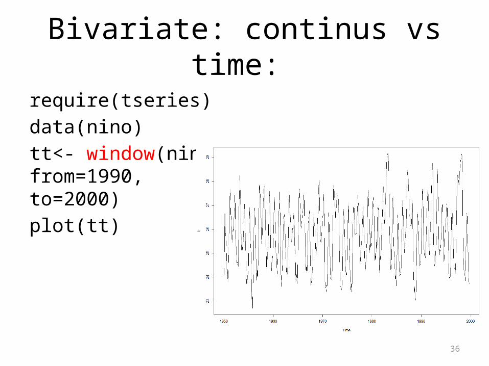
Bivariate: continus vs time:

require(tseries)data(nino)tt<- window(nino3, from=1990, to=2000)plot(tt)

37

# Timeseries - decompostionplot(decompose(nino3))

38

Multivariate data

#Multivariate dataplot(iris, col=iris$Species)

39

Linear model

lm1<- lm(mpg~wt, data=mtcars)par(mfrow=c(2,2))plot(lm1)