1

Building Phylogenetic TreesBuilding Phylogenetic Trees

Yaw-Ling Lin (林耀鈴 )

Dept Computer Sci and Info Management Providence University, Taiwan

E-mail: yllin@pu.edu.twWWW: http://www.cs.pu.edu.tw/~yawlin

2

Phylogenetic Tree

• Topology: bifurcating– Leaves - 1…N

– Internal nodes N+1…2N-2

leaf

branch internal node

3

Orthologues / Paralogues

4

Rooted / Unrooted Tree

5

Counting Trees

6

Counting Trees

(2N - 5)!! = # unrooted trees for N taxa(2N- 3)!! = # rooted trees for N taxa

CA

B D

A B

C

A D

B E

C

A D

B E

C

F

7

Rrooting the tree:

To root a tree mentally, imagine that the tree is made of string. Grab the string at the root and tug on it until the ends of the string (the taxa) fall opposite the root: A

BC

Root D

A B C D

RootNote that in this rooted tree, taxon A is no more closely related to taxon B than it is to C or D.

Rooted tree

Unrooted tree

8

UPGMA -- Unweighted Pair Group Method with Arithmetic mean

simplest method - uses sequential clustering algorithm(assumption of rate constancy among lineages - often violated)

A BB dABC dAC dBC

(AB)C d(AB)C d(AB)C = (dAC + dAB) / 2Distance matrix

Tree

dAB / 2

A

B

A

d(AB)C / 2

B

C

step 1 step 2

9

UPGMA Step 1combine B and C

A B C D EA 0 10 12 10 7B 0 4 4 13C 0 6 15D 0 13E 0

a

e c b

d

10

UPGMA step 2combine BC and D

A BC D EA 0 11 10 7BC 0 5 14D 0 13E 0

(10+12)/2

(4+6)/2

a

e c b

d

2 2

11

UPGMA step 3combine A and E

A BCD EA 0 10.5 7BCD 0 13.5E 0

a

e c b

d

2

2 .5

.5

2

12

UPGMA step 4combine AE and BCD

AE BCDAE 0 12BCD 0

a

e

c b

d

3.5 3.5

2

2 .5

.5

2

13

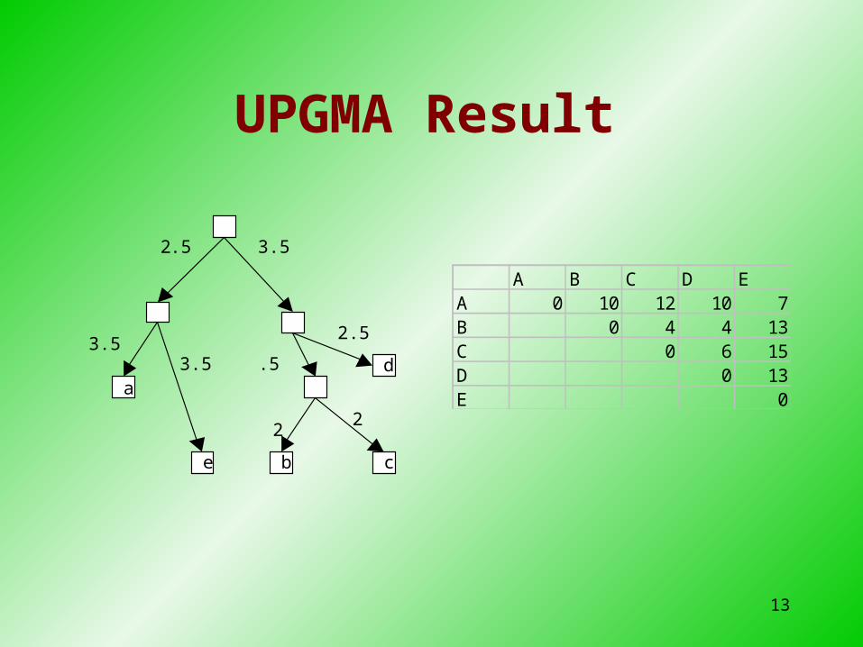
UPGMA Result

A B C D EA 0 10 12 10 7B 0 4 4 13C 0 6 15D 0 13E 0a

e

c b

d 3.5

3.5

2

2.5

.5

2

2 .5

3.5

14

UPGMA Result

a

e

c

b

d 2

3 3

5

3

2

1

1

a

e

c b

d 3.5

3.5

2

2.5

.5

2

2.5

3.5

15

UPGMA(1)

16

UPGMA(2)

17

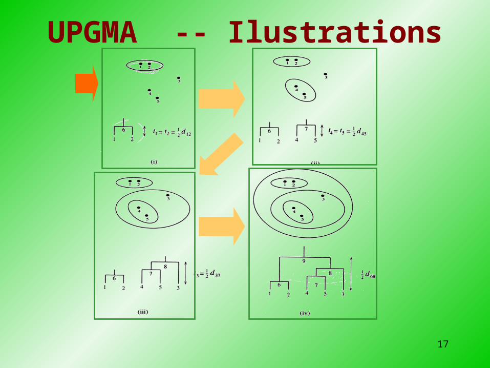
UPGMA -- Ilustrations

18

When UPGMA fails …

19

Neighbor Joining

• Very popular method• Does not make molecular clock assumption : modi

fied distance matrix constructed to adjust for differences in evolution rate of each taxon

• Produces unrooted tree• Assumes additivity: distance between pairs of leav

es = sum of lengths of edges connecting them• Like UPGMA, constructs tree by sequentially join

ing subtrees

20

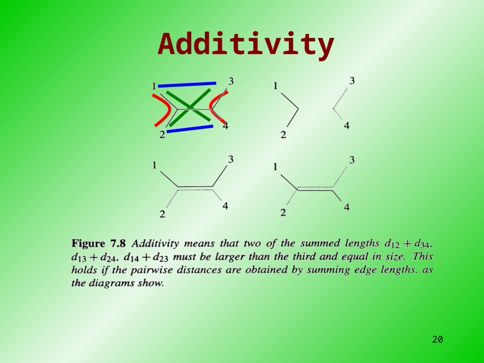
Additivity

21

Naïve NJ by Additivity?

• O(n2) (i,j) pairs

• O(n2) (k,l) pairs

• (k,l) “rejects” (i,j) whenever additivity fails

• O(n4) to pick an (i,j) neighbor pair!

• So totally O(n5) time suffices

22

Neighbor Joining: Once we know the correct (i,j) pair

23

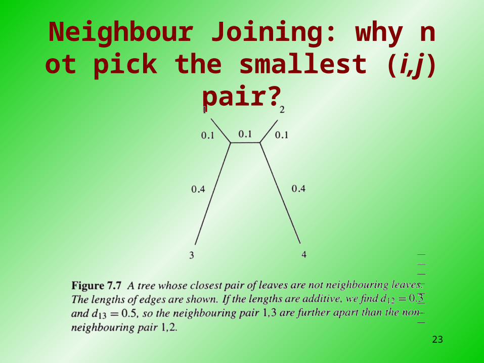
Neighbour Joining: why not pick the smallest (i,j) pair?

26

ik jk i j

ik jk ij

d d r r

d d d

Neighbor-Joining: Algorithm

(A). For each pair , of OTUs, compute

( 2) ( ),

where

(B). Pick a pair , for which is the smallest.

Create a new node and infer distances:

ij ij i j

i ik

k

ij

i j

S N D R R

R D

i j S

k

1 ( ) for ,

2(C). The branch lengths from the new node are

1 [( 2) ]

2( 2)

and

1 [( 2) ]

2( 2)

After deleti

km im jm ij

ik ij i j

jk ij i j

D D D D m i j

D N D R RN

D N D R RN

ng and from and adding , the

process is repeated until the tree is complete

i j D u

i j

i j

k

m

27

Neighbor-Joining: Complexity

• The method performs a search using time O(n2) and using time O(n2) to update distance matrix.

• Giving a total time complexity of O(n3),and a space complexity of O(n2).

28

Reasoning the NJ Method

• How did the ideas of Si,j and Ri comes from ?

• How correct is the algorithm?

• Heuristic or exact solution?

29

The “1-star” Sum of the Branch Lengths

)1/(

1

1

1

NT

DN

LSN

ji

ij

N

i

ixo

• D and L as the distance between OTUs and the branch length between nodes

• Each branch is counted N-1 times when all distances are added

30

The “paired-2-star” Sum of the Branch Lengths

ji

ijiY

N

i

XX

N

i

iYXX

N

k

kkXY

DN

L

DLL

LLLNDDN

L

33

1221

3

21

3

21

3

1

]2))(2()([)2(2

1

31

The “paired-2-star” Tree Size

ji

ij

N

k

kk

N

i

iYXXXY

DN

DDDN

LLLLS

3

12

3

21

3

2112

2

1

2

1)(

)2(2

1

)(

ji

ijiY

N

i

XX

N

i

iYXX

N

k

kkXY

DN

L

DLL

LLLNDDN

L

33

1221

3

21

3

21

3

1

]2))(2()([)2(2

1

33

Before the proof

12 1 2

3

1 2 12

3 3

1 1 2 2

1 1

1 2 1212

( )

1 1 1 ( )

2( 2) 2 2

if and then

2

2( 2) 2

Since is the same for all pairs of and , can be rep

N

XY X X iY

i

N

k k ij

k i j

N N

k k

k k

ij

S L L L L

D D D DN N

R D R D

T R R DS

N

T i j S

laced by

( 2)

for the purpose of computing the relative value.

ij ij i jS N D R R

34

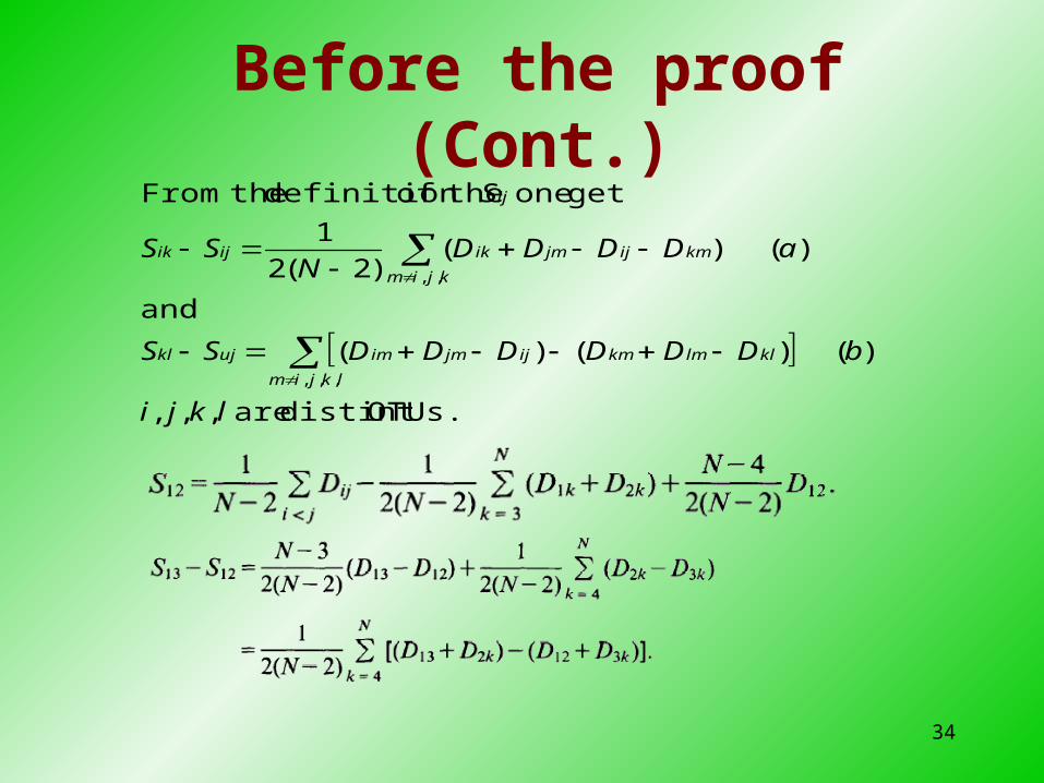
Before the proof (Cont.)

OTUs.distint are ,,,

)( )()(

and

)( )()2(2

1

get one theof definition theFrom

,,,

,,

lkji

bDDDDDDSS

aDDDDN

SS

S

lkjim

kllmkmijjmimujkl

kjim

kmijjmikijik

ij

35

Neighbor-Joining: The proof

neighbors. are and

thenminimum, is that sochosen are and If :

positive. is

)(in summandEach :

column. and row itsin element

leaststrictly is then neighbors, are and If :

positive. are

branches allin which treeaby generated is that Assume

,,

ji

SjiTheorem

DDDDSSproof

SjiLemma

D

ij

kjim

kmijjmikijik

ij

36

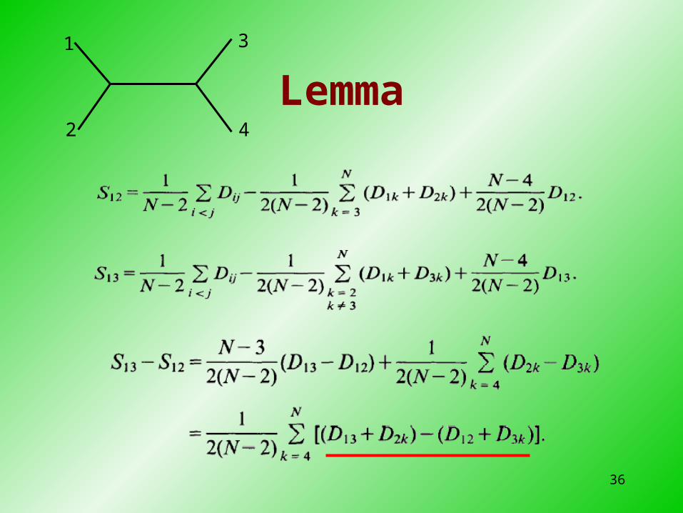
Lemma2

1 3

4

38

Proof

ijik

jmikkmij

kmijjmikijik

SS

DDDD

DDDDSSproofkjim

positive is )(:,,

2

1 3

4

39

Proof of the Theorem: by contradiction

Suppose that i and j are not neighbors. Let k and l be any pair of neighbors, so that i, j, k, and l are distinct and are represented in the tree .Consider the sum in formula (b), which is nonnegative. If m is fifth OUT, then it joins the tree at point x along one of the indicated arcs. Say that m is of type 1 if it joins the path from I to j at any node different from u and that m is of type 2 if it joins the path from i to j at node u.

(b) )()(,,,

lkjim

kllmkmijjmimijkl DDDDDDSS

r

Type1: A = -2Dux-2Duv

Type2: B = -4Dvx+2Duv

For the sum in formula b to be nonnegative, Type2 should be more than Type1.

i

j

k

l

vux

xw

s

x

B

A

40

Proof of the theorem (Cont.)

If m is of type 1,then the corresponding summand in formula (b) is -2Dux-2Duv. If m is of type 2, then the corresponding summand in formula (b) is -4Dvx+2Duv. For the sum in formula (b) to be nonnegative, there must be at least as many terms corresponding to OTUs m of type 2 as there are terms corresponding top OTUs m of type 1. It follows that there are more OTUs that join the path from i to j at u than there are OTUs that join that path at all other nodes combined.

Because neither i nor j has a neighbor, there must be a pair r,s of neighbors that argument applied to w that is different from u, By the above argument applied to w, there are more OTUs that join the path from i to j at w than there are OTUs that join that path at all other nodes combined. The conclusions about u and w contradict each other, and the theorem follows.

41

Speeding up Neighbor-Joining Tree Construction

• In this paper, the authors present several heuristics for speeding up the NJ method.

• The heuristics attempt to reduce the search time by using a quad-tree.

• The worst case time complexity remains O(n3) and the space complexity after adding the quad-tree is still O(n2).

• The authors have implemented a tool, QuickJoin.

42

Previous Work

• The neighbor-joining method is introduced by Saitou and Nei.

• The algorithm was later amended by Studier and Keppler with a running time O(n3).

• BIONJ -- Gascuel et al. produce a O(n3) implementation of a variant of the NJ algorithm that produce more accurate trees in many cases.

• QuickTree -- Durbin et al. produce an code optimized implementation of the NJ algorithm.

44

+/- of distance methods

• Advantages:– easy to perform – quick calculation– fit for sequences having high similarity scores

• Disadvantages:– the sequences are not considered as such (loss of

information) – all sites are generally equally treated (do not take into

account differences of substitution rates ) – not applicable to distantly divergent sequences.

45

Parsimony

46

Maximum Parsimony Method

principle - search for tree that requires the smallest number of character state changes between the OTUs

informative sites - those that favor some trees over others

operationally - at least two different kinds of residuesat the site, each of which isfound in at least two of the OUT sequences

T C A G A T C T A GT T A G A A C T A GT T C G A T C G A GT T C T A A G G A C

SiteOTU 1 2 3 4 5 6 7 8 9 10 1 2 3 4

47

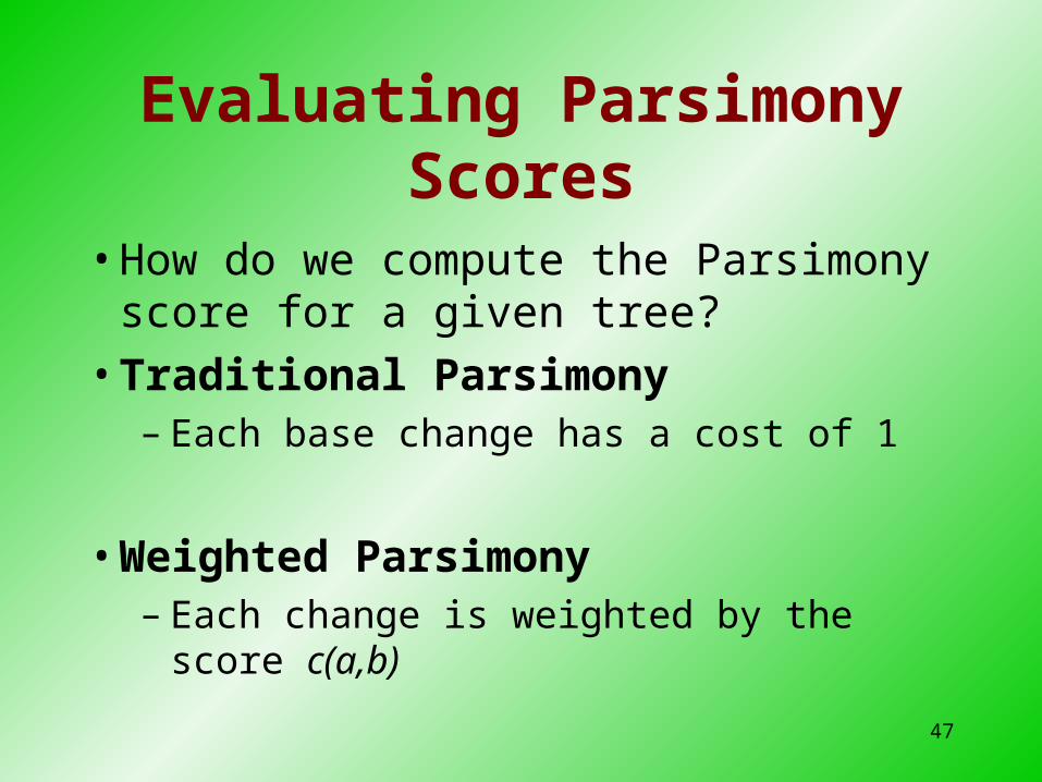
Evaluating Parsimony Scores

• How do we compute the Parsimony score for a given tree?

• Traditional Parsimony– Each base change has a cost of 1

• Weighted Parsimony– Each change is weighted by the score c(a,b)

48

Traditional Parsimony}{

},{nodesinternalmin);,...,(

vu xxEvu

n TssPar

11

a g a

{a,g}

{a}

•Solved independently for each position

•Linear time solution

a

a

49

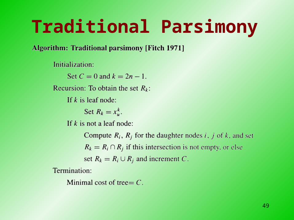
Traditional Parsimony

50

Evaluating Weighted Parsimony

Dynamic programming on the tree

Initialization:

• For each leaf i set S(i,a) = 0 if i is labeled by a, otherwise S(i,a) =

Iteration:

• if k is node with children i and j, then S(k,a) = minb(S(i,b)+c(a,b)) + minb(S(j,b)+c(a,b))

Termination:

• cost of tree is minaS(r,a) where r is the root

k

i j

52

Cost of Evaluating Parsimony

• Score is evaluated on each position independetly. Scores are then summed over all positions.

• If there are n nodes, m characters, and k possible values for each character, then complexity is O(nmk)

• By keeping traceback information, we can reconstruct most parsimonious values at each ancestor node

53

Weighted Parsimony

54

Traditional Parsimony is not “complete”

55

Parsimony: Searching over all trees by Branch and Bound

59

Inferring trees – Maximum Likelihood method

• Maximum likelihood supposes a model of evolution along tree branches.

• Strategy: Find parameters (tree, branch lengths, substitution rate) that

maximizes the likelihood assigned to the data.

• Note: Model of evolution does not include indels!• In Phylip package: program PROTML

60

Probabilistic Methods

• The phylogenetic tree represents a generative probabilistic model (like HMMs) for the observed sequences.

• Background probabilities: q(a)• Mutation probabilities: P(a|b, t)• Models for evolutionary mutations

– Jukes Cantor– Kimura 2-parameter model

• Such models are used to derive the probabilities

61

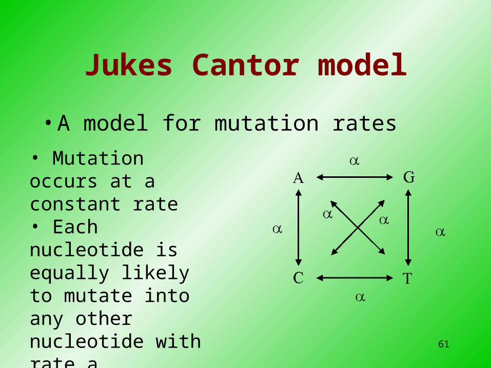
Jukes Cantor model

• A model for mutation rates

• Mutation occurs at a constant rate • Each nucleotide is equally likely to mutate into any other nucleotide with rate a.

62

Kimura 2-parameter model

• Allows a different rate for transitions and transversions.

63

Mutation Probabilities• The rate matrix R is used to derive the mutation probabili

ty matrix S:

• S is obtained by integration. For Jukes Cantor:

• q can be obtained by setting t to infinity

RItS )(

)()(),|(

)()(),|(

tag

taa

etStagP

etStaaP

4

4

14

1

314

1

64

Mutation Probabilities

• Both models satisfy the following properties:

• Lack of memory:

–

• Reversibility:

– Exist stationary probabilities {Pa} s.t.

A

G T

C

b

cbbaca tPtPttP )'()()'(

)()( tPPtPP abbbaa

65

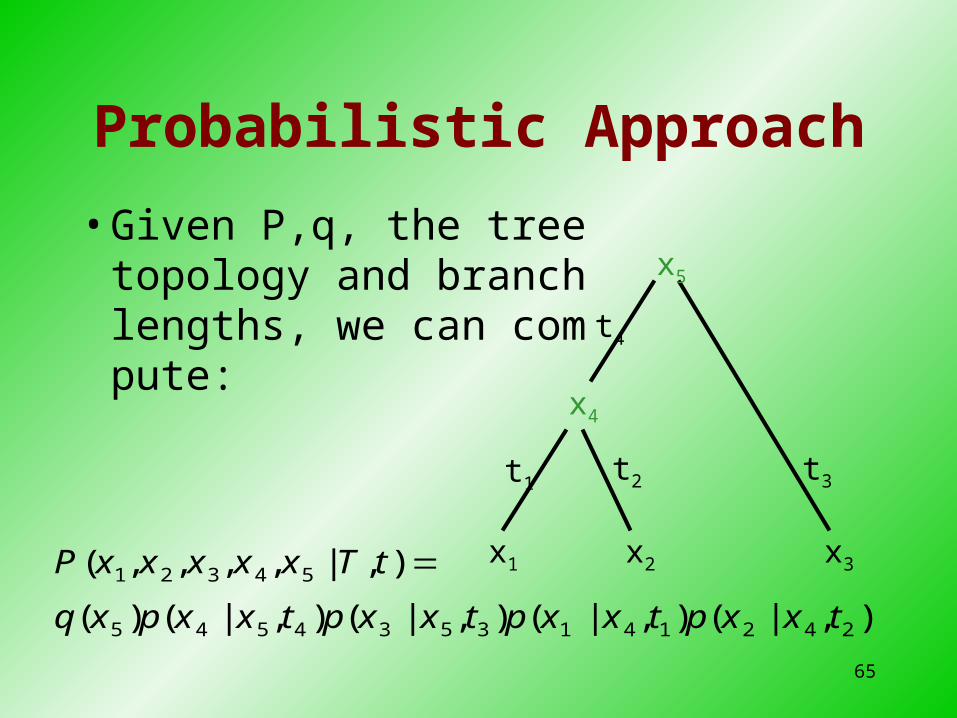
Probabilistic Approach

• Given P,q, the tree topology and branch lengths, we can compute:

),|(),|(),|(),|()(

),|,,,,(

2421413534545

54321

txxptxxptxxptxxpxq

tTxxxxxP x1 x2 x3

x4

x5

t1 t2 t3

t4

66

Computing the Tree Likelihood

54

54321321xx

tTxxxxxPtTxxxP,

),|,,,,(),|,,(

We are interested in the probability of observed data given tree and branch “lengths”:

Computed by summing over internal nodes This can be done efficiently using a tree upward tra

versal pass.

67

Tree Likelihood Computation

• Define P(Lk|a)= prob. of leaves below node k given that xk=a

• Init: for leaves: P(Lk|a)=1 if xk=a ; 0 otherwise

• Iteration: if k is node with children i and j, then

• Termination:Likelihood is

ba

jik cjLtacPbiLtabPaLP,

)|(),|()|(),|()|(

)()|(),|,,( aqaLPtTxxPa

root31

68

Maximum Likelihood (ML)

• Score each tree by – Assumption of independent positions

• Branch lengths t can be optimized– Gradient ascent– EM

• We look for the highest scoring tree– Exhaustive– Sampling methods (Metropolis)

m

nn tTmxmxPtTXXP ),|][,],[(),|,,( 11

69

Optimal Tree Search• Perform search over possible topologies

T1 T3

T4

T2

Tn

Parametric optimization

(EM)

Parameter space

Local Maxima

70

Computational Problem

• Such procedures are computationally expensive!• Computation of optimal parameters, per candidate,

requires non-trivial optimization step.• Spend non-negligible computation on a candidate,

even if it is a low scoring one.• In practice, such learning procedures can only

consider small sets of candidate structures

71

Max Likelihood versus Parsimony

(Example from BSA p. 225)

Choose tree T, with unequal branch lengths.

Generate 1000 sequences of length N according to probabilistic model

(A) Reconstruction by ML (B) Reconstruction by Parsimony

N T1 T2 T3

20 419 339 242

100 638 204 158

500 904 61 35

2000 997 3 0

0.1

0.1

0.09

0.3

0.32

13

4 2

1 3

4 3

1 2

4 2

1 4

3

T1 T2 T3T

N T1 T2 T3

20 396 378 224

100 405 515 79

500 404 594 2

2000 353 646 0

Conclusion: ML infers right tree as N gets larger, Parsimony does not necessarily.

72

Max Likelihood versus NJ

(Example from BSA p. 225)

Choose tree T, with unequal branch lengths.

Generate 1000 sequences of length N according to probabilistic model

(A) Reconstruction by ML (B) Reconstruction by NJ

N T1 T2 T3

20 419 339 242

100 638 204 158

500 904 61 35

2000 997 3 0

0.1

0.10.09

0.3

0.32

13

4 2

1 3

4 3

1 2

4 2

1 4

3T1 T2 T3

T

Conclusion: ML infers right tree as N gets largerl. If the probabilistic model is correct, the ML distances shall be very close to additive, therefore the NJ method predicts the correct tree.

73

Phylip - practicalities

• Menu-driven, no command line• Input file format:

– First line: <number of sequences> <number of letters per sequence>– Next lines: Sequences:

• First ten characters is the sequence name• Then sequence follows. Spaces and newlines are allowed.• Dashes (-) signify gaps

• Example: 4 46hba1 MV-LSPADKTNVKAAWGKVGAHAGEYGAEALERMFLSFPTTKTYFPbeta MVHLTPEEKSAVTALWGKVNVDEVGGEALGRLLVVYPWTQRFFESFMyoglobin –MGLSDGEWQLVLNVWGKVEADIPGHGQEVLIRLFKGHPETLEKFDLeghemogl MGAFSEKQESLVKSSWEAFKQNVPHHSAVFYTLILEKAPAAQNMFS

74

The End