DATA ANALYSIS INCOMMUNITY ANDLANDSCAPE ECOLOGY

Edited by

R. H. G. JONGMAN, C. J. F. TER BRAAK &O. F. R. VAN TONGEREN

CAMBRIDGEUNIVERSITY PRESS

CAMBRIDGE UNIVERSITY PRESSCambridge, New York, Melbourne, Madrid, Cape Town, Singapore, Sao Paulo

Cambridge University Press

The Edinburgh Building, Cambridge CB2 8RU, UK

Published in the United States of America by Cambridge University Press, New York

www.cambridge.orgInformation on this title: www.cambridge.org/9780521475747© Cambridge University Press 1995

This publication is in copyright. Subject to statutory exceptionand to the provisions of relevant collective licensing agreements,no reproduction of any part may take place without the writtenpermission of Cambridge University Press.

First published by Pudoc (Wageningen) 1995New edition with corrections published by Cambridge University Press 1995Tenth printing 2005

A catalogue record for this publication is available from the British Library

Library of Congress Cataloguing in Publication dataData analysis in community and landscape ecology/R.H.G. Jongman,

C.J.F. ter Braak, and O.F.R. van Tongeren, editors. — New ed.p. cm.

Includes bibliographical references (p. ) and index.ISBN 0 521 47574 0 (pbk.)I. Biotic communities-Research-Methodology. 2. Landscapeecology—Research—Methodology. 3. Biotic communities—Research-Statistical methods. 4. Landscape ecology—Research—Statisticalmethods. 5. Biotic communities-Research-Data processing.6. Landscape ecology-Research-Data processing. I. Jongman, R. H. G.II. Braak, C. J. F. ter. III. Van Tongeren, O. F. R.QH541.2.D365 1995574.5'0285-dc20 94-31639 CIP

This reprint is authorized by the original publisher andcopyright holder, Centre for Agricultural Publishing andDocumentation (Pudoc), Wageningen 1987.

ISBN 978-0-521-47574-7 paperback

Transferred to digital printing 2007

Dune Meadow Data

In this book the same set of vegetation data will be used in the chapters onordination and cluster analysis. This set of data stems from a research projecton the Dutch island of Terschelling (Batterink & Wijffels 1983). The objectiveof this project was to detect a possible relation between vegetation and managementin dune meadows. Sampling was done in 1982. Data collection was done by theBraun-Blanquet method; the data are recorded according to the ordinal scaleof van der Maarel (1979b). In each parcel usually one site was selected; onlyin cases of great variability within the parcel were more sites used to describethe parcel. The sites were selected by throwing an object into a parcel. The pointwhere the object landed was fixed as one corner of the site. The sites measure2x2 m2. The sites were considered to be representative of the whole parcel. Fromthe total of 80 sites, 20 have been selected to be used in this book (Table 0.1).This selection expresses the variation in the complete set of data. The namesof the species conform with the nomenclature in van der Meijden et al. (1983)and Tutin et al. (1964-1980).

Data on the environment and land-use that were sampled in this project are(Table 0.2):- thickness of the Al horizon- moisture content of the soil- grassland management type- agricultural grassland use- quantity of manure applied.The thickness of the Al horizon was measured in centimetres and it can thereforebe handled as a quantitative variable. In the dunes, shifting sand is a normalphenomenon. Frequently, young developed soils are dusted over by sand, so thatsoil development restarts. This may result in soils with several Al horizons ontop of each other. Where this had occurred only the Al horizon of the top soillayer was measured.The moisture content of the soil was divided into five ordered classes.lt is thereforean ordinal variable.Four types of grassland management have been distinguished:- standard farming (SF)- biological farming (BF)- hobby-farming (HF)- nature conservation management (NM).The grasslands can be used in three ways: as hayfields, as pasture or a combinationof these (intermediate). Both variables are nominal but sometimes the use of the

grassland is handled as an ordinal variable (Subsection 2.3.1). Therefore a rankingorder has been made from hay production (1), through intermediate (2) tograzing (3).The amount of manuring is expressed in five classes (0-4). It is therefore an ordinalvariable.

All ordinal variables are treated as if they are quantitative, which means thatthe scores of the manure classes, for example, are handled in the same way asthe scores of the Al horizon. The numerical scores of the ordinal variables aregiven in Table 0.2. There are two values missing in Table 0.2 . Some computerprograms cannot handle missing values, so the mean value of the correspondingvariable has been inserted. The two data values are indicated by an asterisk.

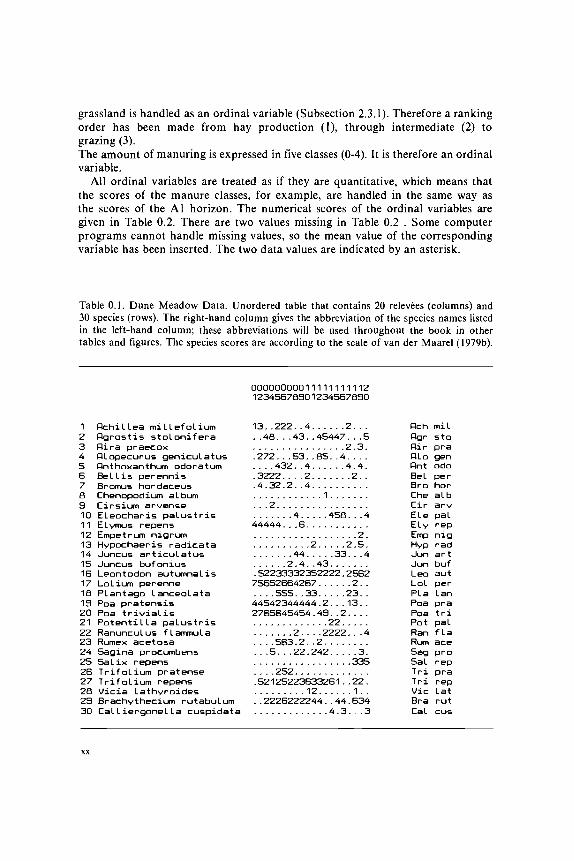
Table 0.1. Dune Meadow Data. Unordered table that contains 20 relevees (columns) and30 species (rows). The right-hand column gives the abbreviation of the species names listedin the left-hand column; these abbreviations will be used throughout the book in othertables and figures. The species scores are according to the scale of van der Maarel (1979b).

OOOOOOOOO1111111111212345678301234567830

1 Rchillea miLLefolium 13..222..4 2... Rchmil2 Rgrostis stoLonifera ..48...43..45447...5 Rgr sto3 Rira praecox 2.3. Rir pra4 Rlopecurus geniculatus .272...53..85..4.... RLo gen5 Rnthoxanthum odoratum ....432..4 4.4. Rnt odo6 Bellis perennis .3222....2 2.. Bel per7 Bromus hordaceus .4.32.2. .4 Bro nor8 Chenopodium album 1 Che alb9 Cirsium arvense . . .2 Cir arv10 ELeocharis palustris 4 458. . .4 ELe pal11 Elymus repens 44444. . .6 Ely rep12 Empetrum nigrum 2. Emp nig13 Hypochaeris radicata 2 2.5. Hyp rad14 Juncus articulatus 44 33. . .4 Jun art15 Juncus bufonius 2.4. .43 Jun buf16 Leontodon autumnal is .52233332352222.2562 Leo aut17 Lolium perenne 75652664267 2.. Lol per18 Plantago lanceolata 555. .33 23. . PLa Ian13 Poa pratensis 44542344444.2... 13. . Poa pra20 Poa trivialis 2765645454.43..2 Poa tri21 Potentilla palustris 22 Pot pal22 Ranunculus f lammula 2. . . .2222. . .4 Ran f La23 Rumex acetosa . . . .563.2. .2 Rum ace24 5agina procumbens . . .5. . .22.242 3. 5ag pro25 5alix repens 335 5al rep26 Trifolium pratense . . . .252 Tri pra27 Trifolium repens .52125223633261..22. Tri rep28 Vicia lathyroides 12 1 . . Vic lat29 Brachythecium rutabulum ..2226222244..44.634 Bra rut30 Calliergonel la cuspidata 4.3. ..3 Cal cus

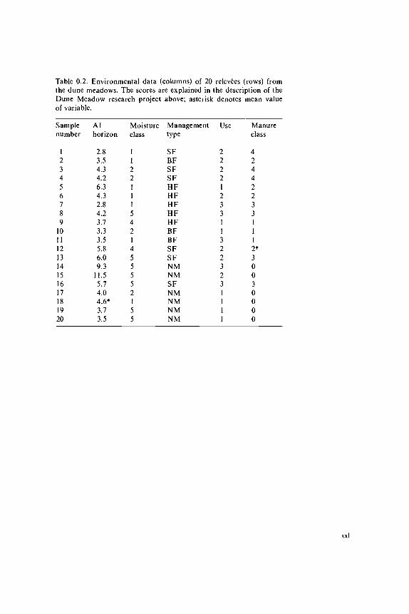
Table 0.2. Environmental data (columns) of 20 relevees (rows) fromthe dune meadows. The scores are explained in the description of theDune Meadow research project above; asterisk denotes mean valueof variable.

Sample Al Moisture Management Use Manurenumber horizon class type class

1 2.8 1 SF 2 423456789

1011121314151617181920

3.54.34.26.34.32.84.23.73.33.55.86.09.3

11.55.74.04.6*3.73.5

1221115421455552155

BFSFSFHFHFHFHFHFBFBFSFSFNMNMSFNMNMNMNM

2221233113223231111

24422331112*30030000

5 Ordination

C.J.F. ter Braak

5.1 Introduction

5.1.1 Aim and usage

Ordination is the collective term for multivariate techniques that arrange sitesalong axes on the basis of data on species composition. The term ordinationwas introduced by Goodall (1954) and, in this sense, stems from the German4Ordnung\ which was used by Ramensky (1930) to describe this approach.

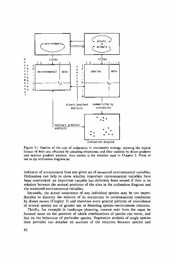
The result of ordination in two dimensions (two axes) is a diagram in whichsites are represented by points in two-dimensional space. The aim of ordinationis to arrange the points such that points that are close together correspond tosites that are similar in species composition, and points that are far apart correspondto sites that are dissimilar in species composition. The diagram is a graphicalsummary of data, as in Figure 5.1, which shows three groups of similar sites.Ordination includes what psychologists and statisticians refer to as multidimen-sional scaling, component analysis, factor analysis and latent-structure analysis.

Figure 5.1 also shows how ordination is used in ecological research. Ecosystemsare complex: they consist of many interacting biotic and abiotic components.The way in which abiotic environmental variables influence biotic compositionis often explored in the following way. First, one samples a set of sites and recordswhich species occur there and in what quantity (abundance). Since the numberof species is usually large, one then uses ordination to summarize and arrangethe data in an ordination diagram, which is then interpreted in the light of whateveris known about the environment at the sites. If explicit environmental data arelacking, this interpretation is done in an informal way; if environmental datahave been collected, in a formal way (Figure 5.1). This two-step approach is indirectgradient analysis in the sense used by Whittaker (1967). By contrast, direct gradientanalysis is impossible without explicit environmental data. In direct gradientanalysis, one is interested from the beginning in particular environmental variables,i.e. either in their influence on the species as in regression analysis (Chapter 3)or in their values at particular sites as in calibration (Chapter 4).

Indirect gradient analysis has the following advantages over direct gradientanalysis. Firstly, species compositions are easy to determine, because species areusually clearly distinguishable entities. By contrast, environmental conditions aredifficult to characterize exhaustively. There are many environmental variables andeven more ways of measuring them, and one is often uncertain of which variablesthe species react to. Species composition may therefore be a more informative

91

enVi

0

nm

nta1

Varla

1s

12

jq

x~ environments.

V. ^si

1 2tes. . i . .

environmental

7

data

ns ^P 2

eci

s

direct g

indirectanalysis

*m

L plants JX

r animals -v

si1 2

tes. . i . . . n

species

y

data

radient summaranalysis

gradient

izing byordination

i* . : •

• *ordination diagram

Figure 5.1 Outline of the role of ordination in community ecology, showing the typicalformat of data sets obtained by sampling ecosystems and their analysis by direct gradientand indirect gradient analysis. Also shown is the notation used in Chapter 5. Point ofsite in the ordination diagram (•).

indicator of environment than any given set of measured environmental variables.Ordination can help to show whether important environmental variables havebeen overlooked: an important variable has definitely been missed if their is norelation between the mutual positions of the sites in the ordination diagram andthe measured environmental variables.

Secondly, the actual occurrence of any individual species may be too unpre-dictable to discover the relation of its occurrence to environmental conditionsby direct means (Chapter 3) and therefore more general patterns of coincidenceof several species are of greater use in detecting species-environment relations.

Thirdly, for example in landscape planning, interest may from the onset befocused more on the question of which combinations of species can occur, andless on the behaviour of particular species. Regression analysis of single speciesthen provides too detailed an account of the relations between species and

92

environment. The ordination approach is less elaborate and gives a global picture,but - one hopes - with sufficient detail for the purpose in hand.

Between regression analysis and ordination (in the strict sense) stand the canonicalordination techniques. They are ordination techniques converted into multivariatedirect gradient analysis techniques; they deal simultaneously with many speciesand many environmental variables. The aim of canonical ordination is to detectthe main pattern in the relations between the species and the observed environment.

5.1.2 Data approximation and response models in ordination

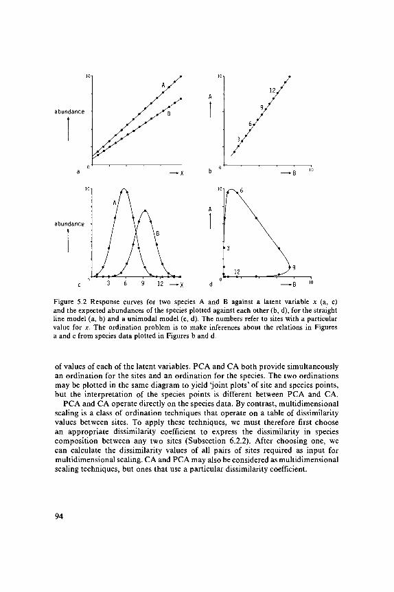
Ordination techniques can be viewed in two ways (Prentice 1977). Accordingto one view, the aim of ordination is to summarize multivariate data in a convenientway in scatter diagrams. Ordination is then considered as a technique for matrixapproximation (as the data are usually presented in the two-way layout of a matrix).A second, more ambitious, view assumes from the beginning that there is anunderlying (or latent) structure in the data, i.e. that the occurrences of all speciesunder consideration are determined by a few unknown environmental variables(latent variables) according to a simple response model (Chapter 3). Ordinationin this view aims to recover that underlying structure. This is illustrated in Figure5.2 for a single latent variable. In Figure 5.2a, the relations of two species, Aand B, with the latent variable are rectilinear. In Figure 5.2c they are unimodal.We now record species abundance values at several sites and plot the abundanceof Species A against that of Species B. If relations with the latent variable wererectilinear, we would obtain a straight line in the plot of Species B against SpeciesA (Figure 5.2b), but if relations were unimodal, we would obtain a complicatedcurve (Figure 5.2d). The ordination problem of indirect gradient analysis is toinfer about the relations with the latent variable (Figures 5.2a,c) from the speciesdata only (Figure 5.2b,d). From the second viewpoint, ordination is like regressionanalysis, but with the major difference that in ordination the explanatory variablesare not known environmental variables, but 'theoretical'variables. These variables,the latent variables, are constructed in such a way that they best explain thespecies data. As in regression, each species thus constitutes a response variable,but in ordination these response variables are analysed simultaneously. (Thedistinction between these two views of ordination is not clear-cut, however. Matrixapproximation implicitly assumes some structure in the data by the mere waythe data are approximated. If the data structure is quite different from the assumedstructure, the approximation is inefficient and fails.)

The ordination techniques that are most popular with community ecologists,are principal components analysis (PCA), correspondence analysis (CA), andtechniques related to CA, such as weighted averaging and detrended correspondenceanalysis. Our introduction to PCA and CA will make clear that PCA and CAare suitable to detect different types of underlying data structure. PCA relatesto a linear response model in which the abundance of any species either increasesor decreases with the value of each of the latent environmental variables (Figure5.2a). By contrast, CA is related, though in a less unequivocal way, to a unimodalresponse model (Figure 5.2c). In this model, any species occurs in a limited range

93

abundance

— X

abundance

c 3 6 9 12 ^ x c

Figure 5.2 Response curves for two species A and B against a latent variable x (a, c)and the expected abundances of the species plotted against each other (b, d), for the straightline model (a, b) and a unimodal model (c, d). The numbers refer to sites with a particularvalue for x. The ordination problem is to make inferences about the relations in Figuresa and c from species data plotted in Figures b and d.

of values of each of the latent variables. PCA and CA both provide simultaneouslyan ordination for the sites and an ordination for the species. The two ordinationsmay be plotted in the same diagram to yield 'joint plots' of site and species points,but the interpretation of the species points is different between PCA and CA.

PCA and CA operate directly on the species data. By contrast, multidimensionalscaling is a class of ordination techniques that operate on a table of dissimilarityvalues between sites. To apply these techniques, we must therefore first choosean appropriate dissimilarity coefficient to express the dissimilarity in speciescomposition between any two sites (Subsection 6.2.2). After choosing one, wecan calculate the dissimilarity values of all pairs of sites required as input formultidimensional scaling. CA and PCA may also be considered as multidimensionalscaling techniques, but ones that use a particular dissimilarity coefficient.

94

5.1.3 Outline of Chapter 5

Section 5.2 introduces CA and related techniques and Section 5.3 PCA. Section5.4 discusses methods of interpreting ordination diagrams with external (envir-onmental) data. It is also a preparation for canonical ordination (Section 5.5).After a discussion of multidimensional scaling (Section 5.6), Section 5.7 evaluatesthe advantages and disadvantages of the various ordination techniques andcompares them with regression analysis and calibration. After the bibliographicnotes (Section 5.8) comes an appendix (Section 5.9) that summarizes the ordinationmethods described in terms of matrix algebra.

5.2 Correspondence analysis (CA) and detrended correspondence analysis (DCA)

5.2.1 From weighted averaging to correspondence analysis

Correspondence analysis (CA) is an extension of the method of weightedaveraging used in the direct gradient analysis of Whittaker (1967) (Section 3.7).Here we describe the principles in words; the mathematical equations will begiven in Subsection 5.2.2.

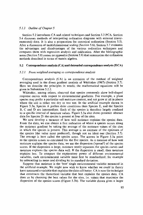
Whittaker, among others, observed that species commonly show bell-shapedresponse curves with respect to environmental gradients. For example, a plantspecies may prefer a particular soil moisture content, and not grow at all in placeswhere the soil is either too dry or too wet. In the artificial example shown inFigure 5.3a, Species A prefers drier conditions than Species E, and the SpeciesB, C and D are intermediate. Each of the species is therefore largely confinedto a specific interval of moisture values. Figure 5.3a also shows presence-absencedata for Species D: the species is present at four of the sites.

We now develop a measure of how well moisture explains the species data.From the data, we can obtain a first indication of where a species occurs alongthe moisture gradient by taking the average of the moisture values of the sitesin which the species is present. This average is an estimate of the optimum ofthe species (the value most preferred), though not an ideal one (Section 3.7).The average is here called the species score. The arrows in Figure 5.3a pointto the species scores so calculated for the five species. As a measure of how wellmoisture explains the species data, we use the dispersion ('spread') of the speciesscores. If the dispersion is large, moisture neatly separates the species curves andmoisture explains the species data well. If the dispersion is small, then moistureexplains less. To compare the explanatory power of different environmentalvariables, each environmental variable must first be standardized; for exampleby subtracting its mean and dividing by its standard deviation.

Suppose that moisture is the 'best' single environmental variable measured inthe artificial example. We might now wish to know whether we could in theoryhave measured a variable that explains the data still better. CA is now the techniquethat constructs the theoretical variable that best explains the species data. CAdoes so by choosing the best values for the sites, i.e. values that maximize thedispersion of the species scores (Figure 5.3b). The variable shown gives a larger

95

1 SD

AE B D Cfolded CA axis

Figure 5.3 Artificial example of unimodal response curves of five species (A-E) with respectto standardized variables, showing different degrees of separation of the species curves,a: Moisture, b: First axis of CA. c: First axis of CA folded in this middle and the responsecurves of the species lowered by a factor of about 2. Sites are shown as dots at y — 1if Species D is present and at y = 0 if Species D is absent. For further explanation, seeSubsections 5.2.1 and 5.2.3.

dispersion than moisture; and consequently the curves in Figure 5.3b are narrower,and the presences of Species D are closer together than in Figure 5.3a.

The theoretical variable constructed by CA is termed the first ordination axisof CA or, briefly, the first CA axis; its values are the site scores on the firstCA axis.

A second and further CA axes can also be constructed; they also maximizethe dispersion of the species scores but subject to the constraint of being uncorrelatedwith previous CA axes. The constraint is intended to ensure that new informationis expressed on the later axes. In practice, we want only a few axes in the hopethat they represent most of the variation in the species data.

So we do not need environmental data to apply CA. CA 'extracts' the ordination

96

axes from the species data alone. CA can be applied not only to presence-absencedata, but also to abundance data; for the species scores, we then simply takea weighted average of the values of the sites (Equation 3.28).

5.2.2 Two-way weighted averaging algorithm

Hill (1973) introduced CA into ecology by the algorithm of reciprocal averaging.This algorithm shows once more that CA is an extension of the method of weightedaveraging.

If we have measured an environmental variable and recorded the speciescomposition, we can estimate for each species its optimum or indicator valueby averaging the values of the environmental variable over the sites in whichthe species occurs, and can use the averages so obtained to rearrange the species(Table 3.9). If the species show bell-shaped curves against the environmentalvariable, the rearranged table will have a diagonal structure, at least if the optimaof the curves differ between the species (Table 3.9). Conversely, if the indicatorvalues of species are known, the environmental variable at a site can be estimatedfrom the species that it contains, by averaging the indicator values of these species(Section 4.3) and sites can be arranged in order of these averages. But, thesemethods are only helpful in showing a clear structure in the data if we knowin advance which environmental variable determines the occurrences of the species.If this is not known in advance, the idea of Hill (1973) was to discover the 'underlyingenvironmental gradient' by applying this averaging process both ways in an iterativefashion, starting from arbitrary initial values for sites or from arbitrary initial(indicator) values for species. It can be shown mathematically that this iterationprocess eventually converges to a set of values for sites and species that do notdepend on the initial values. These values are the site and species scores of thefirst CA axis.

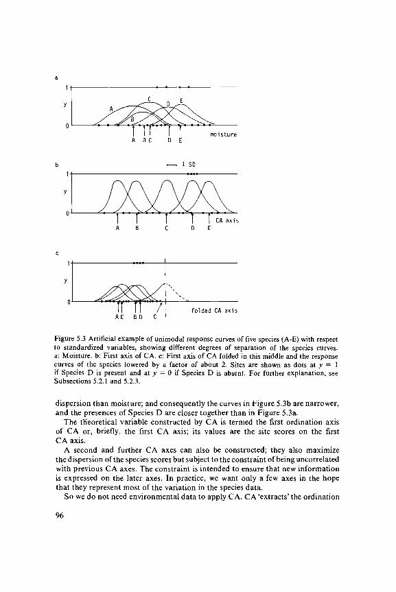
We illustrate now the process of reciprocal averaging. For abundance data,it is rather a process of two-way weighted averaging. Table 5.1a shows the DuneMeadow Data (Table 0.1), arranged in arbitrary order. We take as initial valuesfor the sites the numbers 1 to 20, as printed vertically below Table 5.1a. As before,we shall use the word 'score', instead of 'value'. From the site scores, we derivespecies scores by calculating the weighted average of the site scores for each species.If we denote the abundance of species k at site i by yki, the score of site / byJC, and the score of species k by uk, then the score of species k becomes theweighted average of site scores (Section 3.7)

uk = £"=1 yki xil^v=\ yki Equation 5.1

For Achillea millefolium in Table 5.1a, we obtain u, = ( 1 X 1 + 3 X 2 + 2X 5 + 2 X 6 + 2 X 7 + 4 X 1 0 + 2 X 17)/(1 + 3 + 2 + 2 + 2 + 4 + 2)= 117/16 = 7.31. The species scores thus obtained are also shown in Table 5.1a.F rom these species scores, we derive new site scores by calculating for each sitethe weighted average of the species scores, i.e.

97

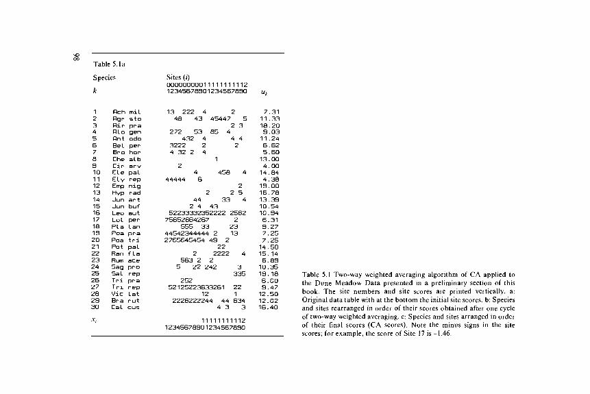
Table 5.1a

Species

k

1234567a3101112131415161718132021222324252627282330

• * /

OchOgrRirRLoRntBelBroCheCirELeELyEmpHypJunJunLeoLoLPlaPoaPoaPotRanRumSagSalTriTriVicBraCal

milstopragenodopernoralbarvpalrepnigradartbufautperIanpratripalf laaceprorepprarepLatrutcus

Sites (i)0000000001111111111212345678901234567890

13 222 4 248 43 45447 5

2 3272 53 85 4

432 4 4 43222 2 24 32 2 4

12

4 458 444444 6

22 2 5

44 33 42 4 43

52233332352222 256275652664267 2

555 33 2344542344444 2 132765645454 49 2

222 2222 4

563 2 25 22 242 3

335252

52125223633261 2212 1

2226222244 44 6344 3 3

1111111111212345678901234567890

uk

7.3111.3318.209.03

11 .246.625.6013.004.0014.844.3819.0016.7813.3910.5410.946.319.277.257.2514.5015. 146.8910.3519. 186.009.4712.5012.0216.40

Table 5.1 Two-way weighted averaging algorithm of CA applied tothe Dune Meadow Data presented in a preliminary section of thisbook. The site numbers and site scores are printed vertically, a:Original data table with at the bottom the initial site scores, b: Speciesand sites rearranged in order of their scores obtained after one cycleof two-way weighted averaging, c: Species and sites arranged in orderof their final scores (CA scores). Note the minus signs in the sitescores; for example, the score of Site 17 is -1.46.

Table 5.

Species

k3 Cir11 ELy7 Bro

26 Tri17 Lol6 Bel23 Rum13 Poa20 Poa1 Rch4 Rio18 PLa27 Tri24 Sag15 Jun16 Leo5 Rnt2 Rgr23 Bra28 Vic8 Che14 Jun21 Pot10 ELe22 Ran30 CaL13 Hyp3 Rir

12 Emp25 5a L

xi

lb

arvrephorpraperperacepratrimilgenLanrepprobufautodostorutlatalbartpalpalflacusradpranigrep

Sites (/)0000001001110111111212534706331288764530

244444 642 3242 2 5

752656662 7 423222 2 25 3 62 2

44254443424 4312766554453 44 2132 242 22 72 35 85 45 535 3 325221265323322 612

5 22242 32 43 4

53223332252352 22624 243 4 448 35 44 744 52222262 4426 4 434

1 2 11

4 4 3 3 422

4 845 42 2 222 4

34 32 2 5

2 32

3 35

1111111167788888833300122234

2430113486773786838356348878043843124736

4.004.385.606.006.316.626.837.257.257.313.033.273.4710.3510.5410.3411.2411.3312.0212.5013.0013.3314.5014.8415.1416.4016.7818.2013.0013.18

Table 5.

Species

k3 Rir5 Rnt1 Rch

26 Tri13 Hyp18 Pla12 Emp7 Bro23 Rum28 Vic6 Bel17 Lol13 Poa11 ELy16 Leo20 Poa27 Tri3 Cir24 Sag15 Jun23 Bra4 RLo8 Che25 Sal2 Rgr14 Jun22 Ran10 ELe21 Pot30 CaL

xi

lc

praodomilpraradLannighoraceLatperperprarepauttrireparvprobufrutgenalbrepstoartflapaLpalcus

Sites (01010001101000110112175076131283432385406

2 344423 4224221 32 252 5225355 3 3

2242 4 35 36 221 2 1

22 322226667 752652 4124434 443544 244 4 4 44623333 655522222322264542 7 655434 22625 235221332216

232 52422

2 4432226 34 62224 24 44

2 723855 41

3 3 548345444574 43 432222424544822433

10000000000000001112

438888666310024 7333065876284411638262250

uk

-0.33-0.36-0.31-0.88-0.84-0.84-0.67-0.66-0.65-0.62-0.50-0.50-0.33-0.37-0.13-0.18-0.08-0.060.000.080. 180.400.420.620.331 .281.561.771.321.36

xt = ! £ , yki uk /S£, yki Equation 5.2

For Site 1 in Table 5.1a, we obtain x, = (1 X 7.31 + 4 X 4.38 + 7 X 6.31+ 4 X 7.25 + 2 X 7.25)/(l + 4 + 7 + 4 + 2 ) = 112.5/18 = 6.25. In Table5.1b, the species and sites are arranged in order of the scores obtained so far.The new site scores are also printed vertically underneath. There is already somediagonal structure, i.e. the occurrences of each species tend to come togetheralong the rows. We can improve upon this structure by calculating new speciesscores from the site scores that we have just calculated, and so on.

A practical numerical problem with this technique is that, by taking averages,the range of the scores gets smaller and smaller. For example, we started offwith a range of 19 (site scores from 1 to 20) and after one cycle the site scoreshave a range of 14.36 - 6.25 = 8.11 (Table 5.1b). To avoid this, either the sitescores or the species scores must be rescaled. Here the site scores have been rescaled.There are several ways of doing so. A simple way is to rescale to a range from0 to 100 by giving the site with the lowest score the value 0 and the site withthe highest score the value 100 and by calculating values for the remaining sitesin proportion to their scores; in the example, the rescaled scores would be obtainedwith the formula (*,. - 6.25)/0.0811.

We shall use another way in which the site scores are standardized to (weighted)

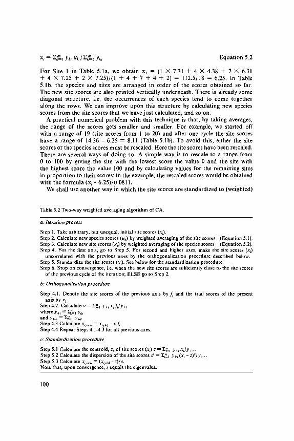
Table 5.2 Two-way weighted averaging algorithm of CA.

a: Iteration process

Step 1. Take arbitrary, but unequal, initial site scores (*;).Step 2. Calculate new species scores (uk) by weighted averaging of the site scores (Equation 5.1).Step 3. Calculate new site scores (x,) by weighted averaging of the species scores (Equation 5.2).Step 4. For the first axis, go to Step 5. For second and higher axes, make the site scores (xt)

uncorrelated with the previous axes by the orthogonalization procedure described below.Step 5. Standardize the site scores (JC,). See below for the standardization procedure.Step 6. Stop on convergence, i.e. when the new site scores are sufficiently close to the site scores

of the previous cycle of the iteration; ELSE go to Step 2.

b: Orthogonalization procedure

Step 4.1. Denote the site scores of the previous axis by ft and the trial scores of the presentaxis by *,-.

Step 4.2. Calculate v = ! £ , y+i *,/•/>'++where y+i = I^Liyki

andj>++=X=i y+fStep 4.3 Calculate JC, new = x, old - v / .Step 4.4 Repeat Steps 4.1-4.3 for all previous axes.c: Standardization procedure

Step 5.1 Calculate the centroid, z, of site scores (x,) z = L£, y+i Xjjy++.Step 5.2 Calculate the dispersion of the site scores s2 = I-5L, y+i (x, - z)2/y++.Step 5.3 Calculate */new = (*/>old - z)/s.Note that, upon convergence, s equals the eigenvalue.

100

mean 0 and variance 1 as described in Table 5.2c. If the site scores are sostandardized, the dispersion of the species scores can be written as

5 = I£L, yk+ uk2/y++ Equation 5.3

whereyk+ is the total abundance of species ky++ the overall total.

The dispersion will steadily increase in each iteration cycle until, after about 10cycles, the dispersion approaches its maximum value. At the same time, the siteand species scores stabilize. The resulting scores have maximum dispersion andthus constitute the first CA axis.

If we had started from a different set of initial site scores or from a set ofarbitrary species scores, the iteration process would still have resulted in the sameordination axis. In Table 5.1c, the species and sites are rearranged in order oftheir scores on the first CA axis and show a clear diagonal structure.

A second ordination axis can also be extracted from the species data. Theneed for a second axis may be illustrated in Table 5.1c; Site 1 and Site 19 lieclose together along the first axis and yet differ a great deal in species composition.This difference can be expressed on a second axis. The second axis is extractedby the same iteration process, with one extra step in which the trial scores forthe second axis are made uncorrelated with the scores of the first axis. This canbe done by plotting in each cycle the trial site scores for the second axis againstthe site scores of the first axis and fitting a straight line by a (weighted) least-squares regression (the weights are y+i/y++). The residuals from this regression(i.e. the vertical deviations from the fitted line: Figure 3.1) are the new trial scores.They can be obtained more quickly by the orthogonalization procedure describedin Table 5.2b. The iteration process would lead to the first axis again withoutthe extra step. The intention is thus to extract information from the species datain addition to the information extracted by the first axis. In Figure 5.4, the finalsite scores of the second axis are plotted against those of the first axis. Site 1and Site 19 lie far apart on the second axis, which reflects their difference inspecies composition. A third axis can be derived in the same way by makingthe scores uncorrelated with the scores of the first two axes, and so on. Table5.2a summarizes the algorithm of two-way weighted averaging. A worked exampleis given in Exercise 5.1 and its solution.

In mathematics, the ordination axes of CA are termed eigenvectors (a vectoris a set of values, commonly denoting a point in a multidimensional space and'eigen' is German for 'self). If we carry out an extra iteration cycle, the scores(values) remain the same, so the vector is transformed into itself, hence, the termeigenvector. Each eigenvector has a corresponding eigenvalue, often denoted byX (the term is explained in Exercise 5.1.3). The eigenvalue is actually equal tothe (maximized) dispersion of the species scores on the ordination axis, and isthus a measure of importance of the ordination axis. The first ordination axishas the largest eigenvalue (^,), the second axis the second largest eigenvalue (k2),

101

Hyp radAi r pra Emp nig

1 1 »Ant odo

2.0-

V i c T a t

Pla Ian <

Ach mil

Leo aut

1811 *

Tr i pra

Rum ace P o a

x

Bel p e r . X « X

Bro hor"« ^ L o l per A3Poa t r i

Ely^rep

Cir arv

-2.0 +

Sal rep

Bra ru t

Sag pro

129 X 13

X X

Jun buf • A l o gen

Che alb

15 vX X

—•• Cal cus20 — - Pot pal

X — - Ele pal— • Ran f l a

14

2.0Agr sto

Figure 5.4 CA ordination diagram of the Dune Meadow Data in Hill's scaling. In thisand the following ordination diagrams, the first axis is horizontal and the second axisvertical; the sites are represented by crosses and labelled by their number in Table 5.1;species names are abbreviated as in Table 0.1.

and so on. The eigenvalues of CA all lie between 0 and 1. Values over 0.5 oftendenote a good separation of the species along the axis. For the Dune MeadowData, Xl = 0.53; X2 = 0.40; X3 = 0.26; X4 = 0.17. As X3 is small compared toX, and X2, we ignore the third and higher numbered ordination axes, and expectthe first two ordination axes to display the biologically relevant information (Figure5.4).

When preparing an ordination diagram, we plot the site scores and the speciesscores of one ordination axis against those of another. Because ordination axesdiffer in importance, one would wish the scores to be spread out most alongthe most important axis. But our site scores do not do so, because we standardizedthem to variance 1 for convenience in the algorithm (Table 5.2). An attractive

102

standardization is obtained by requiring that the average width of the speciescurves is the same for each axis. As is clear from Figure 5.3b, the width of thecurve for Species D is reflected in the spread among its presences along the axis.Therefore, the average curve width along an axis can be estimated from the data.For example, Hill (1979) proposed to calculate, for each species, the varianceof the scores of the sites containing the species and to take the (weighted) averageof the variances so obtained, i.e. Hill proposed to calculate

E* yk+ P i yki (*/ - Uk)2lyk+Vy++-

To equalize the average curve width among different axes, we must thereforedivide all scores of an axis by its average curve width (i.e. by the square rootof the value obtained above). This method of standardization is used in the computerprogram DECORANA (Hill 1979a). Other than in Table 5.2, the program furtheruses the convention that site scores are weighted averages of species scores; sowe must iterate Step 3 of our algorithm once more, before applying the stan-dardization procedure just described. This scaling has already been used inpreparing Figure 5.4 and we shall refer to it as Hill's scaling. A short cut toobtain Hill's scaling from the scores obtained from our algorithm is to dividethe site scores after convergence by y/(l - X)/X and the species scores byyJX(\ - X). The scores so obtained are expressed in multiples of one standarddeviation (s.d.) and have the interpretation that sites that differ by 4 s.d. in scoretend to have few species in common (Figure 5.3b). This use of s.d. will be discussedfurther in Subsection 5.2.4.

CA cannot be applied on data that contain negative values. So the data shouldnot be centred or standardized (Subsection 2.4.4). If the abundance data of eachspecies have a highly skew distribution with many small values and a few extremelylarge values, we recommend transforming them by taking logarithms:loge (yki + 1), as in Subsection 3.3.1. By doing so, we prevent a few high valuesfrom unduly influencing the analysis. In CA, a species is implicitly weighted byits relative total abundance yk+/y++ and, similarly, a site is weighted by y+i/y++.If we want to give a particular species, for example, triple its weight, we mustmultiply all its abundance values by 3. Sites can also be given greater or smallerweight by multiplying their abundance values by constants (ter Braak 1987b).

5.2.3 Diagonal structures: properties and faults of correspondence analysis

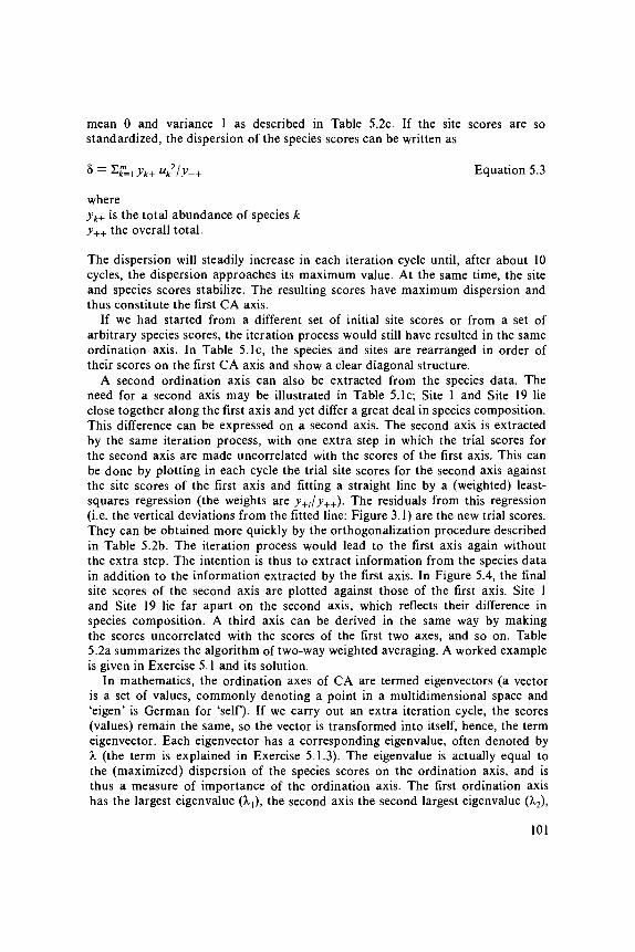
Table 5.3a shows artificial data in which the occurrences of species across sitesappear rather chaotic and Table 5.3b shows the same data after arranging thespecies and sites in order of their score on the first CA axis. The data are rearrangedinto a perfectly diagonal table, also termed a two-way Petrie matrix. (A Petriematrix is an incidence matrix that has a block of consecutive ones in every row;the matrix is two-way Petrie if the matrix also has a block of consecutive onesin every column, the block in the first column starting in the first row and theblock of the last column ending in the last row.) For any table that permitssuch a rearrangement, we can discover the correct order of species and sites from

103

the scores of the first axis of CA. This property of CA can be generalized toquantitative data (Gifi 1981) and to (one-way) Petrie matrices (Heiser 1981; 1986).For two-way Petrie matrices with many species and sites and with about equalnumbers of occurrences per species and per site, the first eigenvalue is closeto 1; e.g. for Table 5.3, A,, = 0.87.

Note that CA does not reveal the diagonal structure if the ones and zerosare interchanged. Their role is asymmetrical, as is clear from the reciprocal averagingalgorithm. The ones are important; the zeros are disregarded. Many ecologistsfeel the same sort of asymmetry between presences and absences of species.

The ordination of Table 5.3 illustrates two 'faults' of CA (Figure 5.5). First,the change in species composition between consecutive sites in Table 5.3, Columnb is constant (one species appears; one disappears) and one would therefore wishthat this constant change were reflected in equal distances between scores ofneighbouring sites along the first axis. But the site scores at the ends of the firstaxis are closer together than those in the middle of the axis (Figure 5.5b). Secondly,the species composition is explained perfectly by the ordering of the sites andspecies along the first axis (Table 5.3, Column b) and the importance of the secondaxis should therefore be zero. However X2 ~ 0-57 and the site scores on thesecond axis show a quadratic relation with those on the first axis (Figure 5.5a).This fault is termed the arch effect. The term 'horseshoe' is also in use but isless appropriate, as the ends do not fold inwards in CA.

Table 5.3 CA applied to artificial data (- denotes absence). Column a: The table lookschaotic. Column b: After rearrangement of species and sites in order of their scores onthe first CA axis (uk and JC,-), a two-way Petrie matrix appears: X{ = 0.87.

Column a

Species

ABCDEFGHI

Sites1 2

1 -1 -1 1- -- 1- 1_ __ _

3

_-----111

4

_--111-_-

5

_--1--11-

6

_--1-11_-

7

_11-1--_-

Column b

Species

ABCEFDGHI

Xi

Sites1

111_--__-

1

40

7

_111--__-

1

08

2

_-111-__-

0

60

4

_-_111__-

0

00

6

_---111_-

0

60

5

_----111-

1

08

3

_-----111

1

40

-1.40-1.24-1.03-0.560.000.561.031.241.40

104

a

-1

- 3 - 2 - 1 0 1 2 3axis 1

Figure 5.5 Ordination by CA of the two-way Petrie matrix of Table 5.3. a: Arch effectin the ordination diagram (Hill's scaling; sites labelled as in Table 5.3; species not shown),b: One-dimensional CA ordination (the first axis scores of Figure a, showing that sitesat the ends of the axis are closer together than sites near the middle of the axis, c: One-dimensional DCA ordination, obtained by nonlinearly rescaling the first CA axis. Thesites would not show variation on the second axis of DCA.

Let us now give a qualitative explanation of the arch effect. Recall that thefirst CA axis maximally separates the species curves by maximizing the dispersion(Equation 5.3) and that the second CA axis also tries to do so but subject tothe constraint of being uncorrelated with the first axis (Subsection 5.2.1). If thefirst axis fully explains the species data in the way of Figure 5.3b, then a possiblesecond axis is obtained by folding the first axis in the middle and bringing theends together (Figure 5.3c). This folded axis has no linear correlation with thefirst axis. The axis so obtained separates the species curves, at least Species Cfrom Species B and D, and these from Species A and E, and is thus a strongcandidate for the second axis of CA. Commonly CA will modify this folded axissomewhat, to maximize its dispersion, but the order of the site and species scoreson the second CA axis will essentially be the same as that of the folded axis.Even if there is a true second underlying gradient, CA will not take it to bethe second axis if its dispersion is less than that of the modified folded first axis.The intention in constructing the second CA axis is to express new information,but CA does not succeed in doing so if the arch effect appears.

5.2.4 Detrended correspondence analysis (DCA)

Hill & Gauch (1980) developed detrended correspondence analysis (DCA) asa heuristic modification of CA, designed to correct its two major 'faults': (1) thatthe ends of the axes are often compressed relative to the axes middle; (2) that

105

the second axis frequently shows a systematic, often quadratic relation with thefirst axis (Figure 5.5). The major of these is the arch effect.

The arch effect is 'a mathematical artifact, corresponding to no real structurein the data' (Hill & Gauch 1980). They eliminate it by 'detrending'. Detrendingis intended to ensure that, at any point along the first axis, the mean value ofthe site scores on the subsequent axes is about zero. To this end, the first axisis divided into a number of segments and within each segment the site scoreson Axis 2 are adjusted by subtracting their mean (Figure 5.6). In the computerprogram DECOR AN A (Hill 1979a), running segments are used for this purpose.This process of detrending is built into the two-way weighted averaging algorithm,and replaces the usual orthogonalization procedure (Table 5.2). Subsequent axesare derived similarly by detrending with respect to each of the existing axes.Detrending applied to Table 5.3 gives a second eigenvalue of 0, as required.

The other fault of CA is that the site scores at the end of the first axis areoften closer together than those in the middle of the axis (Figure 5.5b). Throughthis fault, the species curves tend to be narrower near the ends of the axis thanin the middle. Hill & Gauch (1980) remedied this fault by nonlinearly rescalingthe axis in such a way that the curve widths were practically equal. Hill & Gauch(1980) based their method on the tolerances of Gaussian response curves for thespecies, using the term standard deviation (s.d.) instead of tolerance. They notedthat the variance of the optima of species present at a site (the 'within-site variance')is an estimate of the average squared tolerance of those species. Rescaling musttherefore equalize the within-site variances as nearly as possible. For rescaling,the ordination axis is divided into small segments; the species ordination is expandedin segments with sites with small within-site variance and contracted in segmentswith sites with high within-site variance. Subsequently, the site scores are calculatedby taking weighted averages of the species scores and the scores of sites andspecies are standardized such that the within-site variance equals 1. The tolerancesof the curves of species will therefore approach 1. Hill & Gauch (1980) furtherdefine the length of the ordination axis to be the range of the site scores. Thislength is expressed in multiples of the standard deviation, abbreviated as s.d.

X X X

X

•

•

X

X X

X

•

• •

•

X

X

X X

•

•

• •

X

•

•

X X

X

• •

•

axis 1Figure 5.6 Method of detrending by segments (simplified). The crosses indicate site scoresbefore detrending; the dots are site scores after detrending. The dots are obtained bysubtracting, within each of the five segments, the mean of the trial scores of the secondaxis (after Hill & Gauch 1980).

106

The use of s.d. is attractive: a Gaussian response curve with tolerance 1 risesand falls over an interval of about 4 s.d. (Figure 3.6). Because of the rescaling,most species will about have this tolerance. Sites that differ 4 s.d. in scores cantherefore be expected to have no species in common. Rescaling of the CA axisof Table 5.3 results in the desired equal spacing of the site scores (Figure 5.5c);the length of the axis is 6 s.d.

DC A applied to the Dune Meadow Data gives, as always, the same first eigenvalue(0.53) as CA and a lower second eigenvalue (0.29 compared to 0.40 in CA). Thelengths of the first two axes are estimated as 3.7 and 3.1 s.d., respectively. Becausethe first axis length is close to 4 s.d., we predict that sites at opposite ends ofthe first axis have hardly any species in common. This prediction can be verifiedin Table 5.1c (the order of DC A scores on the first axis is identical to that ofCA); Site 17 and Site 16 have no species in common, but closer sites have oneor more species in common. The DCA ordination diagram (Figure 5.7) showsthe same overall pattern as the CA diagram of Figure 5.4. There are, however,

Ai r pra

Hyp rad

Tr i pra

Emp niq

Sal rep

Sag pro

17 Vic l a t

2

Tri rep

X9 13

20

15

Agr sto*X X14 1 6

Che alb

• A l o gen

Cal cus

• E l e pal

Pot pal

10Poa pra 2

Bel per*

Lol per

4 (SD-units)

Ely rep

Figure 5.7 DCA ordination diagram of the Dune Meadow Data. The scale marks arein multiples of the standard deviation (s.d.).

107

differences in details. The arch seen in Figure 5.4 is less conspicuous, the positionof Sites 17 and 19 is less aberrant. Further, Achillea millefolium is moved froma position close to Sites 2, 5, 6, 7 and 10 to the bottom left of Figure 5.7 andis then closest to Site 1; this move is unwanted, as this species is most abundantin the former group of sites (Table 5.1).

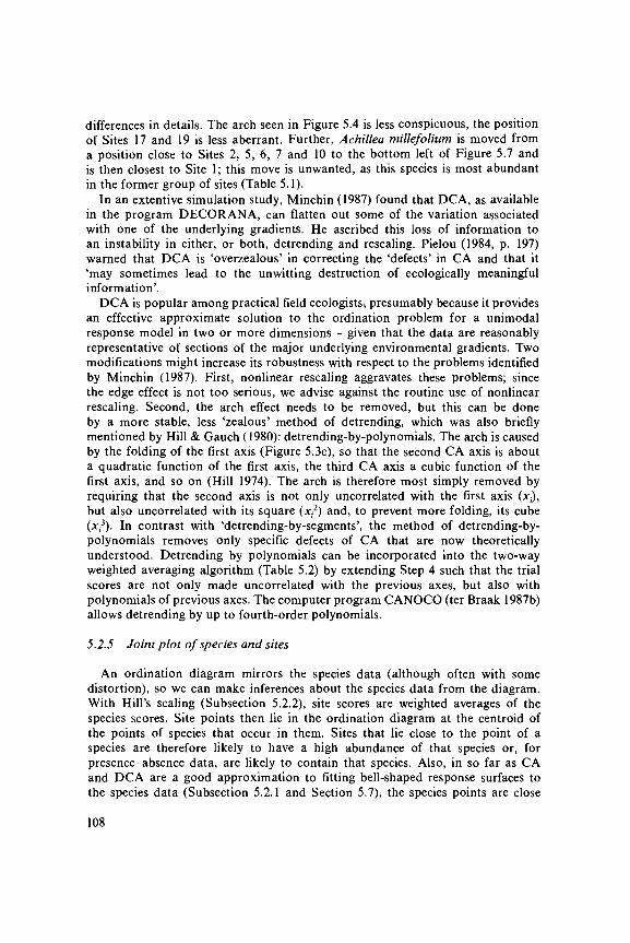
In an extentive simulation study, Minchin (1987) found that DC A, as availablein the program DECORANA, can flatten out some of the variation associatedwith one of the underlying gradients. He ascribed this loss of information toan instability in either, or both, detrending and rescaling. Pielou (1984, p. 197)warned that DCA is 'overzealous' in correcting the 'defects' in CA and that it'may sometimes lead to the unwitting destruction of ecologically meaningfulinformation'.

DCA is popular among practical field ecologists-, presumably because it providesan effective approximate solution to the ordination problem for a unimodalresponse model in two or more dimensions - given that the data are reasonablyrepresentative of sections of the major underlying environmental gradients. Twomodifications might increase its robustness with respect to the problems identifiedby Minchin (1987). First, nonlinear rescaling aggravates these problems; sincethe edge effect is not too serious, we advise against the routine use of nonlinearrescaling. Second, the arch effect needs to be removed, but this can be doneby a more stable, less 'zealous' method of detrending, which was also brieflymentioned by Hill & Gauch (1980): detrending-by-polynomials. The arch is causedby the folding of the first axis (Figure 5.3c), so that the second CA axis is abouta quadratic function of the first axis, the third CA axis a cubic function of thefirst axis, and so on (Hill 1974). The arch is therefore most simply removed byrequiring that the second axis is not only uncorrelated with the first axis (xt),but also uncorrelated with its square (xz

2) and, to prevent more folding, its cube(Xj3). In contrast with 'detrending-by-segments', the method of detrending-by-polynomials removes only specific defects of CA that are now theoreticallyunderstood. Detrending by polynomials can be incorporated into the two-wayweighted averaging algorithm (Table 5.2) by extending Step 4 such that the trialscores are not only made uncorrelated with the previous axes, but also withpolynomials of previous axes. The computer program CANOCO (ter Braak 1987b)allows detrending by up to fourth-order polynomials.

5.2.5 Joint plot of species and sites

An ordination diagram mirrors the species data (although often with somedistortion), so we can make inferences about the species data from the diagram.With Hill's scaling (Subsection 5.2.2), site scores are weighted averages of thespecies scores. Site points then lie in the ordination diagram at the centroid ofthe points of species that occur in them. Sites that lie close to the point of aspecies are therefore likely to have a high abundance of that species or, forpresence-absence data, are likely to contain that species. Also, in so far as CAand DCA are a good approximation to fitting bell-shaped response surfaces tothe species data (Subsection 5.2.1 and Section 5.7), the species points are close

108

to the optima of these surfaces; hence, the expected abundance or probabilityof occurrence of a species decreases with distance from its position in the plot(Figure 3.14).

Using these rules to interpret DCA diagrams, we predict as an example therank order of species abundance for three species from Figure 5.7 and comparethe order with the data in Table 5.1. The predicted rank order for Juncus bufoniusis Sites 12, 8, 13, 9, 18 and 4; in the data Juncus bufonius is present at foursites, in order of abundance Sites 9, 12, 13 and 7. The predicted rank order forRumex acetosa is Sites 5, 7, 6, 10, 2 and 11; in the data R. acetosa occurs infive sites, in order of abundance Sites 6, 5, 7, 9 and 12. Ranunculus flammulais predicted to be most abundant at Sites 20, 14, 15, 16 and less abundant, ifpresent at all, at Sites 8, 12 and 13; in the data, R. flammula is present in sixsites, in order of abundance Sites 20, 14, 15, 16, 8 and 13. We see some agreementbetween observations and predictions but also some disagreement. What is calledfor is a measure of goodness of fit of the ordination diagram. Such a measureis, however, not normally available in CA and DCA.

In interpreting ordination diagrams of CA and DCA, one should be awareof the following aspects. Species points on the edge of the diagram are oftenrare species, lying there either because they prefer extreme (environmental)conditions or because their few occurrences by chance happen to be at sites withextreme conditions. One can only decide between these two possibilities byadditional external knowledge. Such species have little influence on the analysis;if one wants to enlarge the remainder of the diagram, it may be convenient notto display them at all. Further, because of the shortcomings of the method ofweighted averaging, species at the centre of the diagram may either be unimodalwith optima at the centre, or bimodal, or unrelated to the ordination axes. Whichpossibility is most likely can be decided upon by table rearrangement as in Table5.1c or by plotting the abundance of a species against the axes. Species thatlie between the centre and the outer edge are most likely to show a clear relationwith the axes.

5.2.6 Block structures and sensitivity to rare species

CA has attractive properties in the search for block structures. A table is saidto have block structure if its sites and species can be divided into clusters, witheach cluster of species occurring in a single cluster of sites (Table 5.4). For anytable that allows such a clustering, CA will discover it without fail. With thefour blocks in Table 5.4, the first three eigenvalues of CA equal 1 and sites fromthe same cluster have equal scores on the three corresponding axes. An eigenvalueclose to 1 can therefore point to an almost perfect block structure or to a diagonalstructure in the data (Subsection 5.2.3). The search for block structures or 'near-block structures' by CA forms the basis of the cluster-analysis program TWINSPAN(Chapter 6).

This property of CA is, however, a disadvantage in ordination. If a table containstwo disjoint blocks, one of which consists of a single species and a single site,then the first axis of CA finds this questionably uninteresting block. For a similar

109

Table 5.4 Data table with block structure. Outside the Sub-tables A1? A2, A3and A4, there are no presences, so that there are four clusters of sites thathave no species in common (A,, = 1, X,2 — 1, X,3 = 1).

Sites

Species

A,

0

A2

0

A3

A4

reason, CA is sensitive to species that occur only in a few species-poor sites.In the 'down-weighting' option of the program DECOR AN A (Hill 1979a), speciesthat occur in a few sites are given a low weight, so minimizing their influence,but this does not fully cure CA's sensitivity to rare species at species-poor sites.

5.2.7 Gaussian ordination and its relation with CA and DCA

In the introduction to CA (Subsection 5.2.1), we assumed that species showunimodal response curves to environmental variables, intuitively took the dispersionof the species scores as a plausible measure of how well an environmental variableexplains the species data, and subsequently defined CA to be the technique thatconstructs a theoretical variable that explains the species data best in the senseof maximizing the dispersion. Because of the shortcomings of CA noted in thesubsequent sections, the dispersion of the species scores is not ideal to measurethe fit to the species data. We now take a similar approach but with a bettermeasure of fit and assume particular unimodal response curves. We will introduceordination techniques that are based on the maximum likelihood principle(Subsections 3.3.2 and 4.2.1), in particular Gaussian ordination, which is atheoretically sound but computationally demanding technique of ordination. Wealso show that the simpler techniques of CA and DCA give about the same resultif particular additional conditions hold true. This subsection may now be skippedat first reading; it requires a working knowledge of Chapters 3 and 4.

110

One dimension

In maximum likelihood ordination, a particular response model (Subsection3.1.2) is fitted to the species data by using the maximum likelihood principle.In this approach, the fit is measured by the deviance (Subsection 3.3.2) betweenthe data and the fitted curves. Recall that the deviance is inversely related tothe likelihood, namely deviance = -2 loge (likelihood). If we fit Gaussian (logit)curves (Figure 3.9) to the data, we obtain Gaussian ordination. In Subsection3.3.3, we fitted a Gaussian logit curve of pH to the presence-absence data ofa particular species (Figure 3.10). In principle, we can fit a separate curve foreach species under consideration. A measure of how badly pH explains the speciesdata is then the deviance (Table 3.6) summed over all species. Gaussian ordinationof presence-absence data is then the technique that constructs the theoreticalvariable that best explains the species data by Gaussian logit curves, i.e. thatminimizes the deviance between the data and the fitted curves.

A similar approach can be used for abundance data by fitting Gaussian curvesto the data, as in Section 3.4, with the assumption that the abundance data followa Poisson distribution. A Gaussian curve for a particular species has threeparameters: optimum, tolerance and maximum (Figure 3.6), for species k denotedby uk9 tk and ck9 respectively. In line with Equation 3.8, the Gaussian curvescan now be written as

Eyki = ck exp [-0.5(jCi - uk)2/ tk2] Equation 5.4

where x{ is the score of site / on the ordination axis (the value of the theoreticalvariable at site i).

To fit this response model to data we can use an algorithm akin to that to obtainthe ordination axis in CA (Table 5.2).Step 1: Start from initial site scores JC,.Step 2: Calculate new species scores by (log-linear) regression of the species data

on the site scores (Section 3.4). For each species, we so obtain new valuesfor uk, tk and ck.

Step 3: Calculate new site scores by maximum likelihood calibration (Subsection4.2.1).

Step 4: Standardize the site scores and check whether they have changed and,if so, go back to Step 2, otherwise stop.

In this algorithm, the ordination problem is solved by solving the regressionproblem (Chapter 3) and the calibration problem (Chapter 4) in an iterative fashionso as to maximize the likelihood. In contrast to the algorithm for CA, this algorithmmay give different results for different initial site scores because of local maximain the likelihood function for Equation 5.4. It is therefore not guaranteed thatthe algorithm actually leads to the (overall) maximum likelihood estimates; hence,we must supply 'good' initial scores, which are also needed to reduce thecomputational burden. Even for modern computers, the algorithm requires heavycomputation. In the following, we show that a good choice for initial scores are

111

the scores obtained by CA.The CA algorithm can be thought of a simplification of the maximum likelihood

algorithm. In CA, the regression and calibration problems are both solved byweighted averaging. Recall that in CA the species score (uk) is a position onthe ordination axis x indicating the value most preferred by that particular species(its optimum) and that the site score (JC,) is the position of that particular siteon the axis.

We saw in Section 3.7 that the optimum or score of a species (uk) can beestimated efficiently by weighted averaging of site scores provided that (Figure3.18b):Al. the site scores are homogeneously distributed over the whole range ofoccurrence of the species along the axis x.

In Section 4.3, we saw that the score (JC,) of a site is estimated efficiently byweighted averaging of species optima provided the species packing model holds,i.e. provided (Figure 4.1):A2. the species' optima (scores) are homogeneously distributed over a large intervalaround xt.A3. the tolerances of species tk are equal (or at least independent of the optima,ter Braak 1985).A4. the maxima of species ck are equal (or at least independent of the optima;ter Braak 1985).

Under these four conditions the scores obtained by CA approximate themaximum likelihood estimates of the optima of species and the site values inGaussian ordination (ter Braak 1985). For presence-absence data, CA approx-imates similarly the maximum likelihood estimates of the Gaussian logit model(Subsection 3.3.3). CA does not, however, provide estimates for the maximumand tolerance of a species.

A problem is that assumptions Al and A2 cannot be satisfied simultaneouslyfor all sites and species: the first assumption requires that the range of the speciesoptima is amply contained in the range of the site scores whereas the secondassumption requires the reverse. So CA scores show the edge effect of compressionof the end of the first axis relative to the axis middle (Subsection 5.2.3). In practice,the ranges may coincide or may only partly overlap. CA does not give any clueabout which possibility is likely to be true. The algorithm in Table 5.2 resultsin species scores that are weighted averages of the site scores and, consequently,the range of the species scores is contained in the range of the site scores. Butit is equally valid mathematically to stop at Step 3 of the algorithm, so thatthe site scores are weighted averages of the species scores and thus all lie withinthe range of the species scores; this is done in the computer program DECORANA(Hill 1979). The choice between these alternatives is arbitrary. It may helpinterpretation of CA results to go one step further in the direction of the maximumlikelihood estimates by one regression step in which the data of each species areregressed on the site scores of CA by using the Gaussian response model. Thiscan be done by methods discussed in Chapter 3. The result is new species scores(optima) as well as estimates for the tolerances and maxima. As an example,Figure 5.8 shows Gaussian response curves along the first CA axis fitted to the

112

abundance

* CA axis 1

Figure 5.8 Gaussian response curves for some Dune Meadow species, fitted by log-linearregression of the abundances of species (Table 5.1) on the first CA axis. The sites areshown as small vertical lines below the horizontal axis.

Dune Meadow Data in Table 5.1. The curve of a particular species was obtainedby a log-linear regression (Section 3.4) of the data of the species on the site scoresof the first CA axis by using b0 + b{ x + b2 x2 in the linear predictor (Equation3.18).

Two dimensions

In two dimensions, Gaussian ordination means fitting the bivariate Gaussiansurfaces (Figure 3.14)

ki = ck e x P (-0.5[(*n - uki)2 + (*/2 - «*2>2]/'*2) Equation 5.5

where(uku uk2) are the coordinates of the optimum of species k in the ordination diagramck is the maximum of the surfacetk is the tolerance(JC,-, , xi2) are the coordinates of site / in the diagram.

These Gaussian surfaces look like that of Figure 3.14, but have circular contoursbecause the tolerances are taken to be the same in both dimensions.

One cannot hope for more than that the two-axis solution of CA providesan approximation to the fitting of Equation 5.5 if the sampling distribution of

113

the abundance data is Poisson and if:Al. site points are homogeneously distributed over a rectangular region in theordination diagram with sides that are long compared to the tolerances of thespecies,A2. optima of species are homogeneously distributed over the same region,A3. the tolerances of species are equal (or at least independent of the optima),A4. the maxima of species are equal (or at least independent of the optima).

However as soon as the sides of the rectangular region differ in length, thearch effect (Subsection 5.2.3) crops up and the approximation is bad. Figure 5.9bshows the site ordination diagram obtained by applying CA to artificial speciesdata (40 species and 50 sites) simulated from Equation 5.5 with ck — 5 and tk= 1 for each k. The true site points were completely randomly distributed over

4.0

: \•

•

4

• • *•

•

•

•

- • /

• •

•

• * •

•

•

• ••

•

•

•

3.0

2.0

- 4 . 0

Figure 5.9 CA applied to simulated species data, a: True configuration of sites (•). b:Configuration of sites obtained by CA, showing the arch effect. The data were obtainedfrom the Gaussian model of Equation 5.5 with Poisson error, ck — 5, tk = 1 and optimathat were randomly distributed in the rectangle [-1,9] X [-0.5,4.5]. The vertical lines inFigures a and b connect identical sites.

114

a rectangular region with sides of 8 and 4 s.d. (Figure 5.9a). The CA ordinationdiagram is dominated by the arch effect, although the actual position of siteswithin the arch still reflects their position on the second axis in Figure 5.9a. Theconfiguration of site scores obtained by DCA was much closer to the trueconfiguration. DCA forcibly imposes Conditions Al, A2 and A3 upon the solution,the first one by detrending and the second and third one by rescaling of theaxes.

We also may improve the ordination diagram of DCA by going one step furtherin the direction of maximum likelihood ordination by one extra regression step.We did so for the DCA ordination (Figure 5.7) of Dune Meadow Data in Table0.1. For each species with more than 4 presences, we carried out a log-linearregression of the data of the species on the first two DCA axes using the responsemodel

loge Eyki — b0 + blk xn + b3k xa + b4k (xn2 + xi2

2) Equation 5.6

where xi{ and xa are the scores of site / on the DCA axes 1 and 2, respectively.

If bAk < 0, this model is equivalent to Equation 5.5 (as in Subsection 3.3.3).The new species scores are then obtained from the estimated parameters in Equation5.6 by ukj = -blkl(2b,k), uk2 = -b2l(2bik) and tk = 1/\/(-2b<k).

If bAk > 0, the fitted surface shows a minimum and we have just plotted theDCA scores of the species. Figure 5.10a shows how the species points obtainedby DCA change by applying this regression method to the 20 species with fouror more presences. A notable feature is that Achillea millefolium moves towardsits position in the CA diagram (Figure 5.4). In Figure 5.10b, circles are drawnwith centres at the estimated species points and with radius tk. The circles arecontours where the expected abundance is 60% of the maximum expectedabundance ck. Note that exp (-0.5) = 0.60.

From Figure 5.10b, we see, for example, that Trifolium repens has a high tolerance(a large circle, thus a wide ecological amplitude) whereas Bromus hordaceus hasa low tolerance (a small circle, thus a narrow ecological amplitude). With regression,the joint plot of DCA can be interpreted with more confidence. This approachalso leads to a measure of goodness of fit. A convenient measure of goodnessof fit is here

V = 1 - ( I , Dkl)/ ( I , Dk0) Equation 5.7

where Dk0 and Dkl are the residual deviances of the A:th species for the null model(the model without explanatory variables) and the model depicted in the diagram(Equation 5.6), respectively. These deviances are obtained from the regressions(as in Table 3.7). We propose to term V the fraction of deviance accounted forby the diagram. For the two-axis ordination (only partially displayed in Figure5.10b) V = (1 - 360/987) = 0.64. For comparison, V = 0.51 for the one-axisordination (partially displayed in Figure 5.8).

115

Air pra #

Hyp rad

Tri pra

• Emp nig

Sal rep

Sag pro

Cir arv

Jun buf

Ran fla

Jun art , C a 1 cus

Tri rep f

/* / Che alb

/Alo gen

Bel perPoa pra ^

» Ely rep

Figure 5.10 Gaussian response surfaces for several Dune Meadow species fitted by log-linear regression of the abundances of species on the site scores of the first two DCAaxes (Figure 5.7). a: Arrows for species running from their DCA scores (Figure 5.7) totheir fitted optimum, b: Optima and contours for some of the species. The contour indicateswhere the abundance of a species is 60% of the abundance at its optimum.

The regression approach can of course be extended to more complicated surfaces(e.g. Equation 3.24), but this will often be impractical, because these surfacesare more difficult to represent graphically.

5.3 Principal components analysis (PCA)

5.3.1 From least-squares regression to principal components analysis

Principal components analysis (PCA) can be considered to be an extensionof fitting straight lines and planes by least-squares regression. We will introduce

116

4-

Figure 5.10b

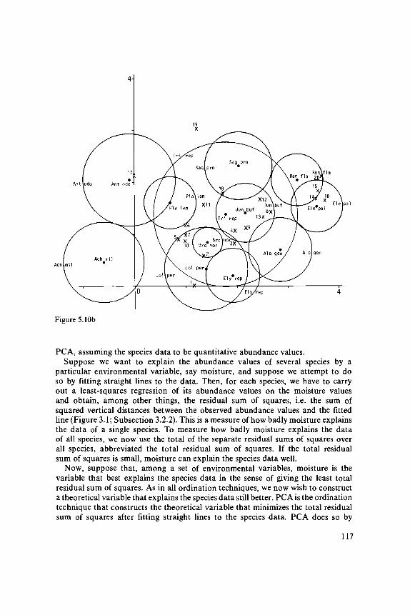
PCA, assuming the species data to be quantitative abundance values.Suppose we want to explain the abundance values of several species by a

particular environmental variable, say moisture, and suppose we attempt to doso by fitting straight lines to the data. Then, for each species, we have to carryout a least-squares regression of its abundance values on the moisture valuesand obtain, among other things, the residual sum of squares, i.e. the sum ofsquared vertical distances between the observed abundance values and the fittedline (Figure 3.1; Subsection 3.2.2). This is a measure of how badly moisture explainsthe data of a single species. To measure how badly moisture explains the dataof all species, we now use the total of the separate residual sums of squares overall species, abbreviated the total residual sum of squares. If the total residualsum of squares is small, moisture can explain the species data well.

Now, suppose that, among a set of environmental variables, moisture is thevariable that best explains the species data in the sense of giving the least totalresidual sum of squares. As in all ordination techniques, we now wish to constructa theoretical variable that explains the species data still better. PCA is the ordinationtechnique that constructs the theoretical variable that minimizes the total residualsum of squares after fitting straight lines to the species data. PCA does so by

117

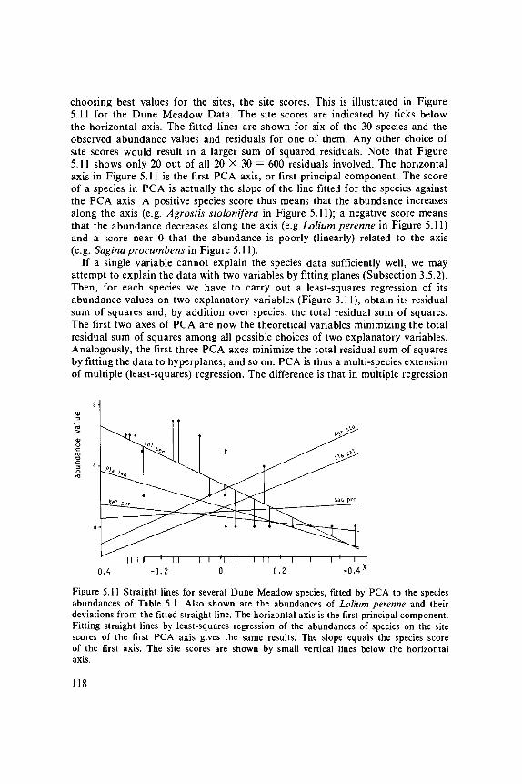
choosing best values for the sites, the site scores. This is illustrated in Figure5.11 for the Dune Meadow Data. The site scores are indicated by ticks belowthe horizontal axis. The fitted lines are shown for six of the 30 species and theobserved abundance values and residuals for one of them. Any other choice ofsite scores would result in a larger sum of squared residuals. Note that Figure5.11 shows only 20 out of all 20 X 30 = 600 residuals involved. The horizontalaxis in Figure 5.11 is the first PCA axis, or first principal component. The scoreof a species in PCA is actually the slope of the line fitted for the species againstthe PCA axis. A positive species score thus means that the abundance increasesalong the axis (e.g. Agrostis stolonifera in Figure 5.11); a negative score meansthat the abundance decreases along the axis (e.g Lolium perenne in Figure 5.11)and a score near 0 that the abundance is poorly (linearly) related to the axis(e.g. Sagina procumbens in Figure 5.11).

If a single variable cannot explain the species data sufficiently well, we mayattempt to explain the data with two variables by fitting planes (Subsection 3.5.2).Then, for each species we have to carry out a least-squares regression of itsabundance values on two explanatory variables (Figure 3.11), obtain its residualsum of squares and, by addition over species, the total residual sum of squares.The first two axes of PCA are now the theoretical variables minimizing the totalresidual sum of squares among all possible choices of two explanatory variables.Analogously, the first three PCA axes minimize the total residual sum of squaresby fitting the data to hyperplanes, and so on. PCA is thus a multi-species extensionof multiple (least-squares) regression. The difference is that in multiple regression

- 0 . 4 '

Figure 5.11 Straight lines for several Dune Meadow species, fitted by PCA to the speciesabundances of Table 5.1. Also shown are the abundances of Lolium perenne and theirdeviations from the fitted straight line. The horizontal axis is the first principal component.Fitting straight lines by least-squares regression of the abundances of species on the sitescores of the first PCA axis gives the same results. The slope equals the species scoreof the first axis. The site scores are shown by small vertical lines below the horizontalaxis.

118

the explanatory variables are supplied environmental variables whereas in PCAthe explanatory variable are theoretical variables estimated from the species dataalone. It can be shown (e.g. Rao 1973) that the same result as above is obtainedby defining the PCA axes sequentially as follows. The first PCA axis is the variablethat explains the species data best, and second and later axes also explain thespecies data best but subject to the constraint of being uncorrelated with previousPCA axes. In practice, we ignore higher numbered PCA axes that explain onlya small proportion of variance in the species data.

5.3.2 Two-way weighted summation algorithm

We now describe an algorithm that has much in common with that of CAand that gives the ordination axes of PCA. The algorithm also shows PCA tobe a natural extension of straight-line regression.

If the relation between the abundance of a species and an environmental variableis rectilinear, we can summarize the relation by the intercept and slope of a straightline. The error part of the model is taken to consist of independent and normallydistributed errors with a constant variance. The parameters (intercept and slope)are then estimated by least-squares regression of the species abundances on thevalues of the environmental variable (Subsection 3.2.2). Conversely, when theintercepts and slopes are known, we can estimate the value of the environmentalvariable from the species abundances at a site by calibration (Subsection 4.2.3).If it is not known in advance which environmental variable determines theabundances of the species, the idea is as in CA (Subsection 5.2.2) to discoverthe 'underlying environmental gradient' by applying straight-line regression andcalibration alternately in an iterative fashion, starting from arbitrary initial valuesfor sites or from arbitrary initial values for the intercepts and slopes of species.As in CA, the iteration process eventually converges to a set of values for speciesand sites that does not depend on the initial values.

The iteration process reduces to simple calculations when we first centre theabundances of each species to mean 0 and standardize the site scores to x =0 and I , (Xj - x)2 = 1. Then, the equations to estimate the intercept and theslope of a straight line (Equations 3.6a,b) reduce to b0 = 0 and bx — I , yt xi9because in the notation of Subsection 3.2.2 y = 0, x = 0 and X, (xt - x)2 —1. Hence we ignore the intercepts and concentrate on the slope parameters. Fromnow on, bk will denote the slope parameter for species k and yki the centredabundance of species k at site / (i.e. yk+ — 0). In this notation, the slope parameterof species k is calculated by

bk = Xfl, y k i xt Equation 5.8

As an example, Table 5.5a shows the Dune Meadow Data used before withan extra column of species means and, as arbitrary initial scores for the sites,values obtained by standardizing the numbers 1 to 20 (bottom row). For Achilleamillefolium, the mean abundance is 0.80 and we obtain

119

to Table 5.o Species

k

1234567

a9101112131415161718192021222324252627282930

RchRgrOirRioRntBelBroCheCirEleElyEmpHypJunJunLeoLoLPlaPoaPoaPotRanRumSag5a LTriTriVicBraCal

5a

milstopragenodoprenoralbarvpaLrepnigradartbufautperLanpratripaLfLaaceprorepprarepLatrutcus

Sites (00000000001111111111212345678901234567890

13 222 4 248 43 45447 5

2 3272 53 85 4

432 4 4 43222 2 24 32 2 4

12

4 458 444444 B

22 2 5

44 33 42 4 43

52233332352222 256275652664267 2

555 33 2344542344444 2 132765645454 49 2

222 2222 4

563 2 25 22 242 3

335252

52125223633261 2212 1

2226222244 44 6344 3 3

00000000000000000000

020110000110000221230001002020

.80

.40

.25

.80

.05

.65

.75

.05

. 10

.25

.30

.10

.45

.90

.65

.70

.90

.30

.40

.15

.20

.70

.90

.00

.55

.45

.35

.20

.45

.50

-1.981.551 .49

-2.060.60-1.96-2.850.10-0.504.21-6.170.662.192.020.020.93-9.42-1.24-6.05-7.930.622.52-2.52-0. 123.70

-1 .57-1.880.312.892.29

3322211100001112223373951740622604715937

Table 5.5 Two-way weighted summation algorithm of PCAapplied to the Dune Meadow Data, a: The original data tablewith at the bottom the initial site scores, b: The species andsites rearranged in order of their scores obtained after one cycleof two-way weighted summation, c: The species arranged in orderof their final scores (PCA scores).

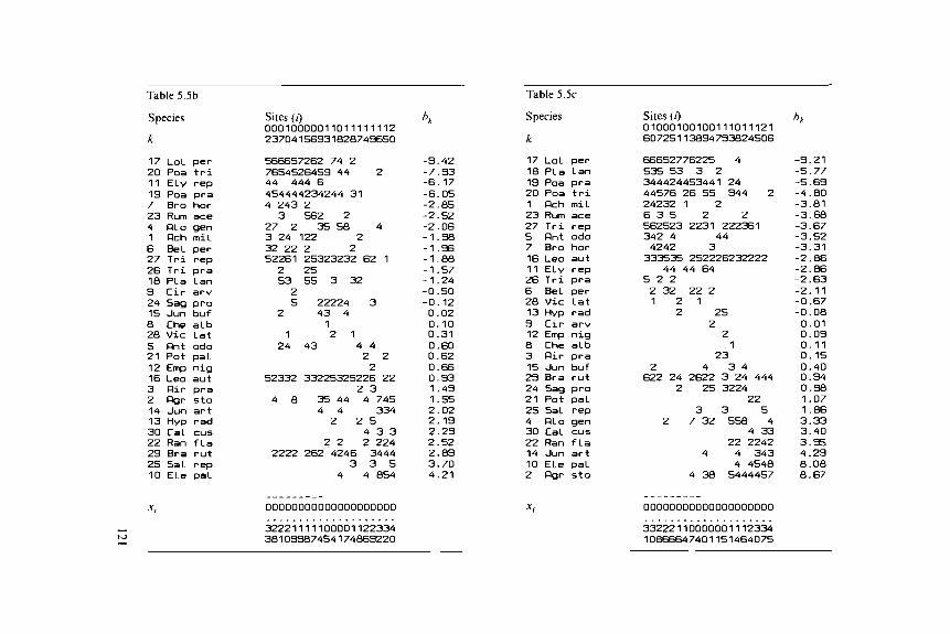
Table 5.5b

Species

k

17 LoL per20 Poa tri11 Ely rep19 Poa pra7 Bro nor23 Rum ace4 OLo gen1 Pen mil6 BeL per27 Tri rep26 Tri pra18 PLa Lan9 Cir arv24 5ag pro15 Jun buf8 Che alb28 Vic Lat5 Ont odo21 Pot pal12 Emp nig16 Leo aut3 Oir pra2 Ogr sto14 Jun art13 Hyp rad30 Cal cus22 Ran fla29 Bra rut25 Sal rep10 ELe pal

xi

Sites (/)0001000001101111111223704156931828749650

566657262 74 27654526459 44 244 444 6454444234244 314 243 23 562 2

27 2 35 58 43 24 122 232 22 2 252261 25323232 62 12 2553 55 3 32

25 22224 3

2 43 41

1 2 124 43 4 4

2 22

52332 33225325226 222 3

4 8 35 44 4 7454 4 3342 2 5

4 3 32 2 2 224

2222 262 4246 34443 3 5

4 4 854

00000000000000000000

3222111110000112233438103987454174869220

-9.42-7.93-6. 17-6.05-2.85-2.52-2.06-1 .98-1 .96-1 .88-1.57-1.24-0.50-0. 120.020.100.310.600.620.660.931 .491.552.022.192.292.522.893.704.21

Table 5.

Species

k

17 LoL18 PLa19 Poa20 Poa1 Och23 Rum27 Tri5 Ont7 Bro16 Leo11 Ely26 Tri6 BeL28 Vic13 Hyp9 Cir12 Emp8 Che3 Oir15 Jun23 Bra24 5ag21 Pot25 5a L4 OLo30 Cal22 Ran14 Jun10 Ele2 Ogr

xi

5c

perLanpratrimilacerepodohorautreppraperlatradarvnigalbprabufrutpropalrepgencusfLaartpaLsto

Sites (i)0100010010011101112160725113894793824506

66652776225 4535 53 3 2344424453441 2444576 26 55 944 224232 1 26 3 5 2 2562523 2231 222361342 4 444242 3333535 252226232222

44 44 645 2 22 32 22 21 2 1

2 252

21

232 4 3 4622 24 2622 3 24 444

2 25 322422

3 3 52 7 32 558 4

4 3322 2242

4 4 3434 4548

4 38 5444457

00000000000000000000

3322211000000111233410866647401151464075

bk

-9.21-5.77-5.69-4.80-3.81-3.68-3.67-3.52-3.31-2.86-2.86-2.63-2.11-0.67-0.080.010.090. 110. 150.400.940.981 .071.863.333.403.954.298.088.67

bl = (1 - 0.80) X (-0.37) + (3 - 0.80) X (-0.33) + (0 - 0.80) X (-0.29) + ...+ (0-0.80) X (0.37) = -1.98.

From the slopes thus obtained (Table 5.5a, last column), we derive new sitescores by least-squares calibration (Equation 4.2 with ak — 0). The site scoresso obtained are proportional to

xi — ^k=\yki bk Equation 5.9

because the denominator of Equation 4.1 has the same value for each site. Thisdenominator is unimportant in PCA, because the next step in the algorithm isto standardize the site scores, as shown in Table 5.6c. For Site 1 in Table 5.5a,we get from Equation 5.9 the site score xx = (1 - 0.80) X (-1.98) + (0 - 2.40)X (1.55) + (0 - 0.25) X (1.49) + ... + (0 - 0.50) X (2.29) = -0.19. Note thatthe species mean abundance is subtracted each time from the abundance value.In Table 5.5b, the species and sites are arranged in order of the scores obtainedso far, in which the slopes (bk) form the species scores. The abundance of thespecies in the top row (Lolium perenne) has the tendency to decrease along therow, whereas the abundance of the species in the bottom row ( Eleocharis palustris)has the tendency to increase across the row. The next cycle of the iteration isto calculate new species scores (bk), then new site scores, and so on. As in CA,the scores stabilize after several iterations and the resulting scores (Table 5.5c)constitute the first ordination axis of PCA. In Table 5.5c, the species and sitesare arranged in order of their scores on the first axis. Going from top row tobottom row, we see first a decreasing trend in abundance across the columns(e.g. for Lolium perenne), then hardly any trend (e.g. for Sagina procumbens)and finally an increasing trend (e.g. for Agrostis stolonifera). A graphical displayof the trends has already been shown in Figure 5.11. The order of species inTable 5.5c is quite different from the order in the table arranged by CA (Table5.1c), but the difference in ordering of the sites is more subtle.

In the above iteration algorithm of PCA (Table 5.6), weighted sums (Equations5.8 and 5.9) replace the weighted averages in CA (Table 5.2; Equations 5.1 and5.2). For this analogy to hold, let us consider the data yki as weights (whichcan be negative in PCA), so that the species scores are a weighted sum of thesite scores and, conversely, the site scores are a weighted sum of the species scores(Table 5.6). The standard terminology used in mathematics is that xt is a linearcombination of the variables (species) and that bk is the loading of species k.

After the first axis, a second axis can be extracted as in CA, and so on. (Thereis a subtle difference in the orthogonalization procedure, which need not concernus here.) The axes are also eigenvectors to which correspond eigenvalues as inCA (Subsection 5.2.2). The meaning of the eigenvalues in PCA is given below.The axes are also termed principal components.

So PCA decomposes the observed values into fitted values and residuals(Equations 3.1 and 3.2). In one dimension, we have the decomposition

yki = bk Xj + residual Equation 5.10

122

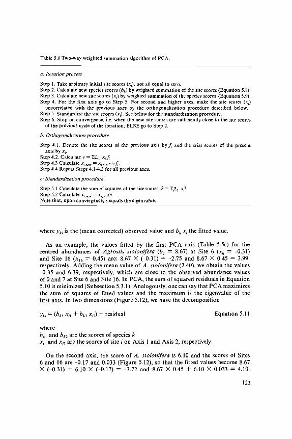
Table 5.6 Two-way weighted summation algorithm of PC A.

a: Iteration process

Step 1. Take arbitrary initial site scores (JC,), not all equal to zero.Step 2. Calculate new species scores (bk) by weighted summation of the site scores (Equation 5.8).Step 3. Calculate new site scores (JC,) by weighted summation of the species scores (Equation 5.9).Step 4. For the first axis go to Step 5. For second and higher axes, make the site scores (JC,)

uncorrelated with the previous axes by the orthogonalization procedure described below.Step 5. Standardize the site scores (JC,). See below for the standardization procedure.Step 6. Stop on convergence, i.e. when the new site scores are sufficiently close to the site scores

of the previous cycle of the iteration; ELSE go to Step 2.

b: Orthogonalization procedure

Step 4.1. Denote the site scores of the previous axis b y / and the trial scores of the presentaxis by JC,.

Step 4.2. Calculate v = ££, JC,/.Step 4.3 Calculate jc,new = jc,old - v/J.Step 4.4 Repeat Steps 4.1-4.3 for all previous axes.

c: Standardization procedure

Step 5.1 Calculate the sum of squares of the site scores s2 = ! £ , JC,2.Step 5.2 Calculate jc,new = xiiOiJs.Note that, upon convergence, s equals the eigenvalue.

where yki is the (mean corrected) observed value and bk xt the fitted value.

As an example, the values fitted by the first PCA axis (Table 5.5c) for thecentred abundances of Agrostis stolonifera (b2 = 8.67) at Site 6 (x6 = -0.31)and Site 16 (JC16 = 0.45) are: 8.67 X (-0.31) = -2.75 and 8.67 X 0.45 = 3.99,respectively. Adding the mean value of A. stolonifera (2.40), we obtain the values-0.35 and 6.39, respectively, which are close to the observed abundance valuesof 0 and 7 at Site 6 and Site 16. In PCA, the sum of squared residuals in Equation5.10 is minimized (Subsection 5.3.1). Analogously, one can say that PCA maximizesthe sum of squares of fitted values and the maximum is the eigenvalue of thefirst axis. In two dimensions (Figure 5.12), we have the decomposition

yki = (bkl xn + bkl xi2) + residual Equation 5.11

wherebkl and bk2 are the scores of species kxn and xa are the scores of site / on Axis 1 and Axis 2, respectively.

On the second axis, the score of A. stolonifera is 6.10 and the scores of Sites6 and 16 are -0.17 and 0.033 (Figure 5.12), so that the fitted values become 8.67X (-0.31) + 6.10 X (-0.17) = -3.72 and 8.67 X 0.45 + 6.10 X 0.033 = 4.10.

123

Alo gen

Lol pei

x b-scale

X-scale

Figure 5.12 PCA-ordination diagram of the Dune Meadow Data in covariance biplot scalingwith species represented by arrows. The b scale applies to species, the x scale to sites.Species not represented in the diagram lie close to the origin (0,0).

The first two PCA axes thus give approximate abundance values of -3.72 + 2.40= -1.3 and 4.10 + 2.40 = 6.5, slightly worse values than those obtained fromthe first axis, but most of the remaining abundance values in the data table willbe approximated better with two axes than with a single axis. The sum of squaresof fitted values now equals X{+ X2. Further, the total sum of squares (£*£,- yk?)equals the sum of all eigenvalues. (This equality means that we can reconstructthe observed values exactly from the scores of species and sites on all eigenvectorsand the mean abundance values.) The fraction of variance accounted for (explained)by the first two axes is therefore (k{ + >.2)/(sum of all eigenvalues). This measureis the equivalent of R2 in Section 3.2. For the Dune Meadow Data, X{ = 471,\2 = 344 and the total sum of squares = 1598. So the two-axes solution explains(471 + 344)/1598 = 51% of the variance. The first axis actually explains 471/1598 = 29% of the variance and the second axis 344/1598 = 22%.

124

5.3.3 Best lines and planes in m-dimensional space

Here we present a geometric approach to PCA. In this approach, the aim ofPCA is seen as being to summarize multivariate data in a graphical way. Theapproach is best illustrated with data on two species only. Figure 5.13a displaysthe abundances of Species A and B at 25 sites in the form of a scatter diagram,with axes labelled by the species names. The simplest summary of data is bythe mean abundances of A (25) and B (15). Knowing the means, we may shiftthe axes to the centroid of the data points, i.e. to the point with the coordinates(25,15), provided we remember that the origin (0,0) of the new coordinate systemis the point (25,15) in the old coordinate system. Next we draw a line throughthe new origin in the direction of maximum variance in the plot. This line isthe first principal component (PCI), or first PCA axis, and perpendicularly wedraw PC2. Next we rotate the plot, so that PCI is horizontal (Figure 5.13b).Figure 5.13b is an ordination diagram with arrows representing the species. Thesearrows are the shifted and rotated axes of the species in the original diagram.PC2 shows so much less variation than PCI that PC2 can possibly be neglected.This is done in Figure 5.13c showing a one-dimensional ordination; the pointsin Figure 5.13c were obtained from Figure 5.13b by drawing perpendicular linesfrom each point on the horizontal axis (projection onto PCI). In this way, thefirst coordinate of the points in Figure 5.13b is retained in Figure 5.13c; thiscoordinate is the site score on PCI. The first coordinate of the arrows in Figure5.13b is the species loading on PCI, which is also represented by an arrow inFigure 5.13c. These arrows indicate the direction in which Species A and SpeciesB increase in abundance; hence Figure 5.13c still shows which sites have highabundances of Species A and of Species B (those on the right side) and whichsites have low abundance (those on the left side).

The example is, of course, artificial. Usually there are many species (m ^ 3),so that we need an ra-dimensional coordinate system, and we want to derivea two-dimensional or three-dimensional ordination diagram. Yet the principleremains the same: PCA searches for the direction of maximum variance; thisis PCI, the best line through the data points. It is the best line in the sensethat it minimizes the sum of squares of perpendicular distances between the datapoints and the line (as is illustrated in Figure 5.13a for m — 2). So the firstcomponent in Figure 5.13a is neither the regression line of Species B on SpeciesA nor that of Species A on Species B, because regression minimizes the sumof squares of vertical distances (Figure 3.1). But, as we have seen in Subsection5.3.1, PCA does give the best regression of Species A on PCI and of SpeciesB on PCI (Figure 5.11). After the first component, PCA seeks the direction ofmaximum variance that is perpendicular onto the first axis; that is PC2, whichwith PCI forms the best plane through the data points, and so on. In general,the site scores are obtained by projecting each data point from the ra-dimensionalspace onto the PCA axes and the species scores are obtained by projecting theunit vectors: for the first species (1,0,0,...); for the second species (0,1,0,0,...), etc.,onto the PCA axes (Figure 5.13).

125

species A

b

x-20

X

'x x - V oxx

10x '

X

X,

XX

-10

c• a>

o

I"ou

"O

seco

i

//

/

/

X

i X

x

X

X

1 x t10X

X

f i rs t component20

X

-20

species B• species A

xxx—x—x̂ x—x-x xx—|-xxxx—x—xxxx—x|x x

-10 0 10 20

Figure 5.13 Artificial abundance data for two species A and B at 25 sites, a: First principalcomponent, running through the centroid of the sites in the direction of the greatest variance(at 34° of the axis of Species A), b: Rotated version of Figure a with the first principalcomponent horizontally, c: One-dimensional PCA ordination with species represented byarrows. The scores are simply those of the first axis of b.

126

5.3.4 Biplot of species and site scores

The scores obtained from a PCA for species and sites can be used to preparea biplot (Gabriel 1971). The biplot serves the same function as the joint plotin CA (Subsection 5.2.5), but the rules to interpret the biplot are rather different.We limit the discussion to the two-dimensional biplot as it is more difficult tovisualize three-dimensional or higher ones. The prefix 'bi' in biplot refers to thejoint representation of sites and species, and not to the dimension of the plot;for example, Figure 5.13c shows a one-dimensional biplot.

The ranges of the scores for sites and for species (scores and loadings) in PCAare often of a different order of magnitude. For example in Table 5.3c, the rangeof the species scores is 17.9 whereas the range of the site scores is 0.8. A biplotis therefore constructed most easily by drawing separate plots of sites and ofspecies on transparent paper, each one with its own scaling. In each of the plots,the scale unit along the vertical axis must have the same physical length as thescale unit along the horizontal axis, as in CA. A biplot is obtained by superimposingthe plots with the axes aligned. A biplot may therefore have different scale unitsfor the sites (x scale) and species (b scale). Figures 5.12 and 5.15 provide examplesfor the Dune Meadow Data.

In Subsection 5.3.1, we showed that for each species PCA fits a straight linein one dimension to the (centred) abundances of the species (Figure 5.11; Equation5.10) and in two dimensions a plane with respect to the PCA axes (Figure 3.11;Equation 5.11). The abundance of a species as fitted by PCA thus changes linearlyacross the biplot. We represent the fitted planes in a biplot by arrows as shownin Figure 5.12. The direction of the arrow indicates the direction of steepest ascentof the plane, i.e. the direction in which the abundance of the corresponding speciesincreases most, and the length of the arrow equals the rate of change in thatdirection. In the perpendicular direction, the fitted abundance is constant. Thearrows are obtained by drawing lines that join the species points to the origin,the point with coordinates (0,0).

The fitted abundances of a species can be read from the biplot in very muchthe same way as from a scatter diagram, i.e. by projecting each site onto theaxis of the species. (This is clear from Figure 5.13a.) The axis of a species ina biplot is in general, however, not the horizontal axis or the vertical axis, asin Figure 5.13a, but an oblique axis, the direction of which is given by the arrowof the species. As an example of how to interpret Figure 5.12, some of the sitepoints are projected onto the axis of Agrostis stolonifera in Figure 5.14. Withoutdoing any calculations, we can see the ranking of the fitted abundances of A.stolonifera among the sites from the order of the projection points of the sitesalong the axis of that species. From Figure 5.14, we thus infer that the abundanceof A. stolonifera is highest at Site 16, second highest at Site 13, and so on toSite 6, which has the lowest inferred abundance. The inferred ranking is not perfectwhen compared with the observed ranking, but not bad either.

Another useful rule to interpret a biplot is that the fitted value is positive ifthe projection point of a site lies, along the species' axis, on the same side ofthe origin as the species point does, and negative if the origin lies between the

127

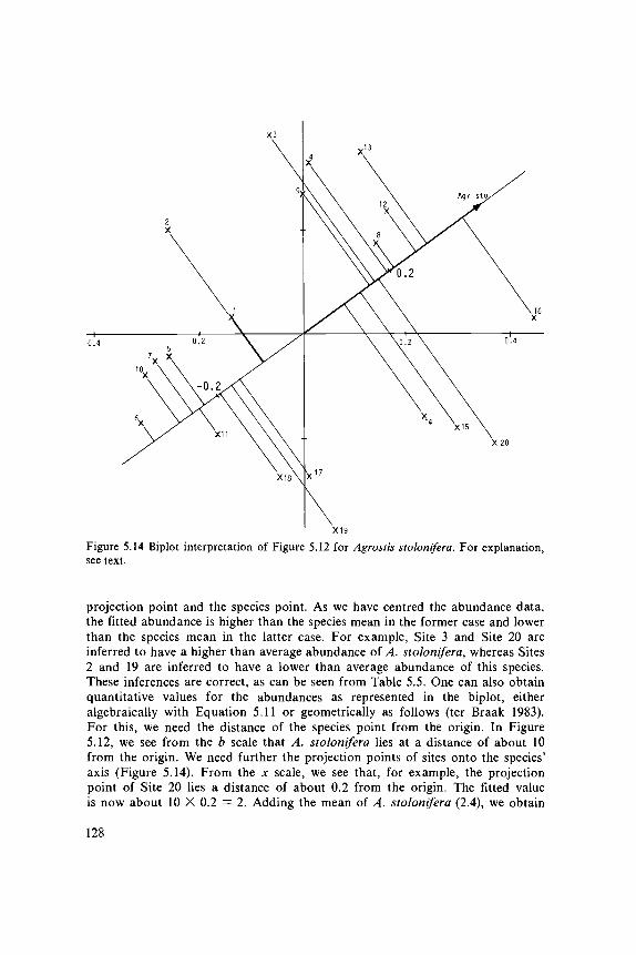
X 20

Figure 5.14 Biplot interpretation of Figure 5.12 for Agrostis stolonifera. For explanation,see text.

projection point and the species point. As we have centred the abundance data,the fitted abundance is higher than the species mean in the former case and lowerthan the species mean in the latter case. For example, Site 3 and Site 20 areinferred to have a higher than average abundance of A. stolonifera, whereas Sites2 and 19 are inferred to have a lower than average abundance of this species.These inferences are correct, as can be seen from Table 5.5. One can also obtainquantitative values for the abundances as represented in the biplot, eitheralgebraically with Equation 5.11 or geometrically as follows (ter Braak 1983).For this, we need the distance of the species point from the origin. In Figure5.12, we see from the b scale that A. stolonifera lies at a distance of about 10from the origin. We need further the projection points of sites onto the species'axis (Figure 5.14). From the x scale, we see that, for example, the projectionpoint of Site 20 lies a distance of about 0.2 from the origin. The fitted valueis now about 10 X 0.2 = 2. Adding the mean of A. stolonifera (2.4), we obtain

128

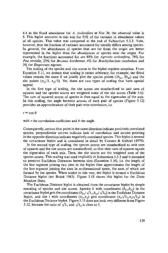
4.4 as the fitted abundance for A. stolonifera at Site 20; the observed value is5. This biplot accounts in this way for 51% of the variance in abundance valuesof all species. This value was computed at the end of Subsection 5.3.2. Note,however, that the fraction of variance accounted for usually differs among species.In general, the abundances of species that are far from the origin are betterrepresented in the biplot than the abundances of species near the origin. Forexample, the fractions accounted for are 80% for Agrostis stolonifera, 78% forPoa trivialis, 25% for Bromus hordaceus, 4% for Brachythecium rutabulum and3% for Empetrum nigrum.

The scaling of the species and site scores in the biplot requires attention. FromEquation 5.11, we deduce that scaling is rather arbitrary; for example, the fittedvalues remain the same if we jointly plot the species points (3b kl, 5bk2) and thesite points (xn/3, xi2/5). Yet, there are two types of scaling that have specialappeal.

In the first type of scaling, the site scores are standardized to unit sum ofsquares and the species scores are weighted sums of the site scores (Table 5.6).The sum of squared scores of species is then equal to the eigenvalue of the axis.In this scaling, the angle between arrows of each pair of species (Figure 5.12)provides an approximation of their pair-wise correlation, i.e.

r « cos 0

with r the correlation coefficient and 6 the angle.

Consequently, arrows that point in the same direction indicate positively correlatedspecies, perpendicular arrows indicate lack of correlation and arrows pointingin the opposite direction indicate negatively correlated species. This biplot is termedthe covariance biplot and is considered in detail by Corsten & Gabriel (1976).

In the second type of scaling, the species scores are standardized to unit sumof squares and the site scores are standardized, so that their sum of squares equalsthe eigenvalue of each axis. Then, the site scores are the weighted sum of thespecies scores. This scaling was used implicitly in Subsection 5.3.3 and is intendedto preserve Euclidean Distances between sites (Equation 5.16), i.e. the length ofthe line segment joining two sites in the biplot then approximates the length ofthe line segment joining the sites in w-dimensional space, the axes of which areformed by the species. When scaled in this way, the biplot is termed a EuclideanDistance biplot (ter Braak 1983). Figure 5.15 shows this biplot for the DuneMeadow Data.

The Euclidean Distance biplot is obtained from the covariance biplot by simplerescaling of species and site scores. Species k with coordinates (bkhbk2) in thecovariance biplot gets the coordinates {bkll\J\x,bk2l V ^ ) m t n e Euclidean Distancebiplot, and site / with coordinates (xn,xa) gets coordinates (xiX\JXx,xi2\/X2) inthe Euclidean Distance biplot. Figure 5.15 does not look very different from Figure5.12, because the ratio of v ^ i and V^-21S close to 1.

129

•10

Ely rep

Poa pra

Lol per

Bro hor Bel per

- 0 . 5 X Tri rep

l o gen

13

Agr sto

Jun buf

Sag pro

Cir arv Jun a r tChe alb * b S C a 1 e

Rum ace • Vic l a t

X X Ach mi l * T r i *p ra

10X Leo#aut

Hyp radPla Ian

Ant odo

• ° i p a l Ran'fi X scaleEmp nig • . E l e pal> Cal cusAir pra

« Sal repBra rut Y

14

Figure 5.15 Euclidean Distance biplot of Dune Meadow Data.

5.3.5 Data transformation

We have so far described the standard form of PCA as treated in statisticaltextbooks (e.g. Morrison 1967). In ecology, this form is known as 'species-centredPCA'. In a variant of this, 'standardized PCA', abundances of each species arealso divided by its standard deviation. In species-centred PCA, each species isimplicitly weighted by the variance of its abundance values. Species with highvariance, often the abundant ones, therefore dominate the PCA solution, whereasspecies with low variance, often the rare ones, have only minor influence on thesolution. This may be reason to apply standardized PCA, in which all speciesreceive equal weight. However the rare species then unduly influence the analysisif there are a lot of them, and chance can dominate the results. We thereforerecommend species-centred PCA, unless there is strong reason to use standardizedPCA. Standardization is necessary if we are analysing variables that are measuredin different units, for example quantitative environmental variables such as pH,mass fraction of organic matter or ion concentrations. Noy Meir et al. (1975)fully discuss the virtues and vices of various data transformations in PCA.

The fraction of variance accounted for by the first few axes is not a measure

130

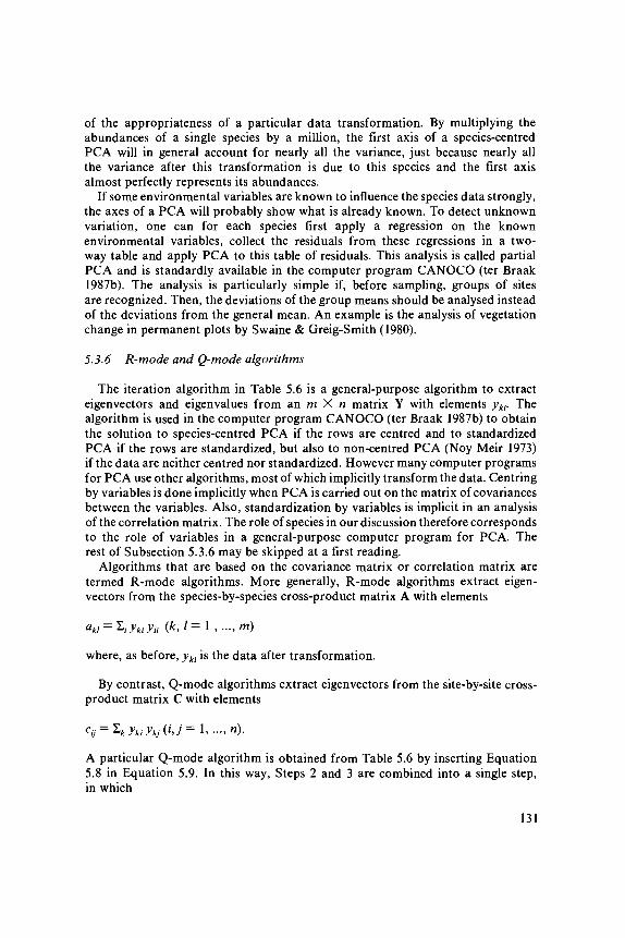
of the appropriateness of a particular data transformation. By multiplying theabundances of a single species by a million, the first axis of a species-centredPCA will in general account for nearly all the variance, just because nearly allthe variance after this transformation is due to this species and the first axisalmost perfectly represents its abundances.

If some environmental variables are known to influence the species data strongly,the axes of a PCA will probably show what is already known. To detect unknownvariation, one can for each species first apply a regression on the knownenvironmental variables, collect the residuals from these regressions in a two-way table and apply PCA to this table of residuals. This analysis is called partialPCA and is standardly available in the computer program CANOCO (ter Braak1987b). The analysis is particularly simple if, before sampling, groups of sitesare recognized. Then, the deviations of the group means should be analysed insteadof the deviations from the general mean. An example is the analysis of vegetationchange in permanent plots by Swaine & Greig-Smith (1980).

5.3.6 R-mode and Q-mode algorithms

The iteration algorithm in Table 5.6 is a general-purpose algorithm to extracteigenvectors and eigenvalues from an m X n matrix Y with elements yki. Thealgorithm is used in the computer program CANOCO (ter Braak 1987b) to obtainthe solution to species-centred PCA if the rows are centred and to standardizedPCA if the rows are standardized, but also to non-centred PCA (Noy Meir 1973)if the data are neither centred nor standardized. However many computer programsfor PCA use other algorithms, most of which implicitly transform the data. Centringby variables is done implicitly when PCA is carried out on the matrix of covariancesbetween the variables. Also, standardization by variables is implicit in an analysisof the correlation matrix. The role of species in our discussion therefore correspondsto the role of variables in a general-purpose computer program for PCA. Therest of Subsection 5.3.6 may be skipped at a first reading.

Algorithms that are based on the covariance matrix or correlation matrix aretermed R-mode algorithms. More generally, R-mode algorithms extract eigen-vectors from the species-by-species cross-product matrix A with elements

aki = ^iykiyii (k,l= l , . . . , m)

where, as before, yki is the data after transformation.

By contrast, Q-mode algorithms extract eigenvectors from the site-by-site cross-product matrix C with elements

A particular Q-mode algorithm is obtained from Table 5.6 by inserting Equation5.8 in Equation 5.9. In this way, Steps 2 and 3 are combined into a single step,in which

131

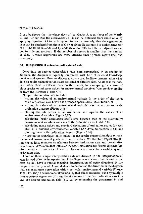
It can be shown that the eigenvalues of the Matrix A equal those of the MatrixC, and further that the eigenvectors of C can be obtained from those of A byapplying Equation 5.9 to each eigenvector and, conversely, that the eigenvectorsof A can be obtained from those of C by applying Equation 5.8 to each eigenvectorof C. The terms R-mode and Q-mode therefore refer to different algorithms andnot to different methods. If the number of species is smaller than the numberof sites, R-mode algorithms are more efficient than Q-mode algorithms, andconversely.

5.4 Interpretation of ordination with external data

Once data on species composition have been summarized in an ordinationdiagram, the diagram is typically interpreted with help of external knowledgeon sites and species. Here we discuss methods that facilitate interpretation whendata on environmental variables are collected at different sites. Analogous methodsexist when there is external data on the species, for example growth form ofplant species or indicator values for environmental variables from previous studiesor from the literature (Table 5.7).

Simple interpretative aids include:- writing the values of an environmental variable in the order of site scores

of an ordination axis below the arranged species data table (Table 5.7)- writing the values of an environmental variable near the site points in the

ordination diagram (Figure 5.16)- plotting the site scores of an ordination axis against the values of an

environmental variable (Figure 5.17)- calculating (rank) correlation coefficients between each of the quantitative

environmental variables and each of the ordination axes (Table 5.8)- calculating mean values and standard deviations of ordination scores for each

class of a nominal environmental variable (ANOVA, Subsection 3.2.1) andplotting these in the ordination diagram (Figure 5.16).

An ordination technique that is suited for the species composition data extractstheoretical environmental gradients from these data. We therefore expect straightline (or at least monotonic) relations between ordination axes and quantitativeenvironmental variables that influence species. Correlation coefficients are thereforeoften adequate summaries of scatter plots of environmental variables againstordination axes.

Three of these simple interpretative aids are directed to the interpretation ofaxes instead of to the interpretation of the diagram as a whole. But the ordinationaxes do not have a special meaning. Interpretation of other directions in thediagram is equally valid. A useful idea is to determine the direction in the diagramthat has maximum correlation with a particular environmental variable (Dargie1984). For theyth environmental variable, zj9 that direction can be found by multiple(least-squares) regression of Zj on the site scores of the first ordination axis (x{)and the second ordination axis (x2), i.e. by estimating the parameters bx and

132

Table 5.7 Values of environmental variables and Ellenberg's indicator values of specieswritten alongside the ordered data table of the Dune Meadow Data, in which species andsites are arranged in order of their scores on the second DC A axis. Al: thickness of Alhorizon (cm), 9 meaning 9 cm or more; moisture: moistness in five classes from 1 = dryto 5 = wet; use: type of agricultural use, 1 = hayfield, 2 = a mixture of pasture andhayfield, 3 = pasture; manure: amount of manure applied in five classes from 0 = nomanure to 5 = heavy use of manure. The meadows are classified by type of management:SF, standard farming; BF, biological farming; HF, hobby farming; NM, nature management;F, R, N refer to Ellenberg's indicator values for moisture, acidity and nutrients, respectively.

Species Site (/)

OOOO1OOOO1O11111112112350749638162485709

FRN

11171761920262321184

a102721530149222829165242513312

j

12345678

flch milEly repBro horLot perBel perPoa praPoa triTri praRum acePot palPla IanRio genChe albEle palTri repRgr stoJun bufCal cusJun artCir arvRan flaVic latBra rutLeo autRnt odoSag proSal repHyp radRir praEmp nig

R1moistureusemanureSFBFHFNM

13 242 2 24444 464 2423756266526 47 23222 2 2445244443244 3 127664555494 24

2 2 55 3 26 2

2 2535 5 3

27 23 55 4814 8 4 5 4

52262135223 3621 24 83 54 744 4 5

2 4 3 43 4 3

4 4 3 3 42

22 2 2 2 41 2 1

2222226 2444 64 4352333223235 2252226442 3 4 4

52 222 4 33 53

2 2 52 3

2

3446334446446695944411212124155154515255222113212233323121114242134123313200000010100010010011000000010010000001000000000001010110100000000000000000000000111111

45

5

57

1039410

67

8

92

5

6

526

3

7

3

33

57

434

58375

7

52277

75

2722

5

6

31

133

Table 5.8 Correlation coefficients (100 X r) of en-vironmental variables with the first four DCA axesfor the Dune Meadow Data.

Variable

1 Al2 moisture3 use4 manure5 SF6 BF7 HF8 NM

Eigenvalue

Axes

1

587635

622

-28-22

21

0.54

2

2457

-21-68-29-24-26

73

0.29

3

77

-3-7

539

-5517

0.08

4

9-7-5

-64-6022

-1456

0.05

4 t

BF .HF

NM

SF

x0 3

X X

Figure 5.16 The amount of manure written on the DCA ordination of Figure 5.7. Thetrend in the amount across the diagram is shown by an arrow, obtained by a multipleregression of manure on the site scores of the DCA axes. Also shown are the mean scoresfor the four types of management, which indicate, for example, that the nature reserves(NM) tend to lie at the top of the diagram.

134

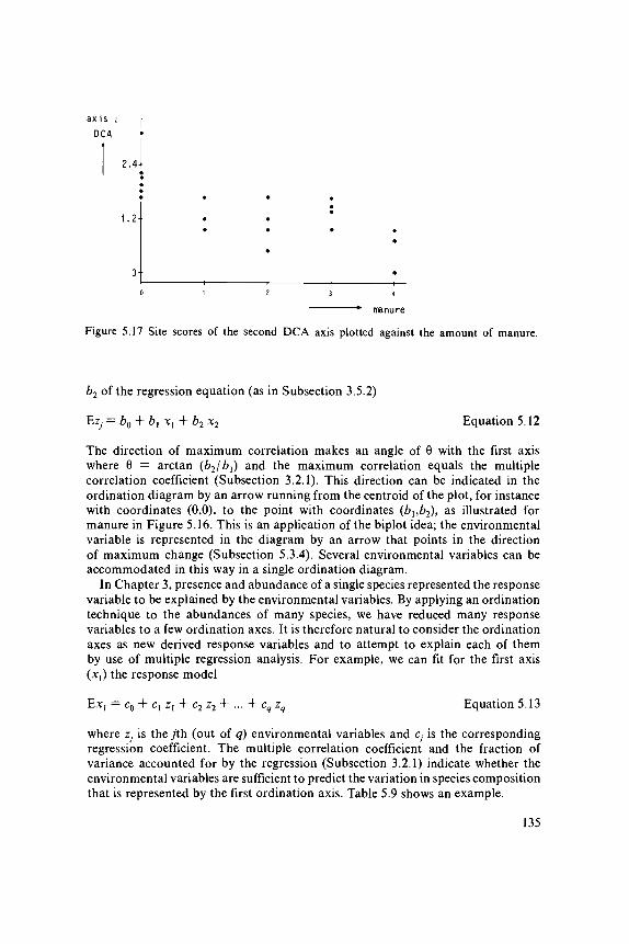
a x i s 2 |

DCA

2.4

1.2-

o-

manure

Figure 5.17 Site scores of the second DCA axis plotted against the amount of manure.

b2 of the regression equation (as in Subsection 3.5.2)

Ezj = b0 + b{ xx + b2 x2 Equation 5.12

The direction of maximum correlation makes an angle of 0 with the first axiswhere 0 = arctan (62/^i) a n d the maximum correlation equals the multiplecorrelation coefficient (Subsection 3.2.1). This direction can be indicated in theordination diagram by an arrow running from the centroid of the plot, for instancewith coordinates (0,0), to the point with coordinates (bhb2), as illustrated formanure in Figure 5.16. This is an application of the biplot idea; the environmentalvariable is represented in the diagram by an arrow that points in the directionof maximum change (Subsection 5.3.4). Several environmental variables can beaccommodated in this way in a single ordination diagram.

In Chapter 3, presence and abundance of a single species represented the responsevariable to be explained by the environmental variables. By applying an ordinationtechnique to the abundances of many species, we have reduced many responsevariables to a few ordination axes. It is therefore natural to consider the ordinationaxes as new derived response variables and to attempt to explain each of themby use of multiple regression analysis. For example, we can fit for the first axis(x,) the response model

Ex, = c0 + cx z, + c2 z2 + ... + cq zq Equation 5.13

where z; is the y'th (out of q) environmental variables and cy is the correspondingregression coefficient. The multiple correlation coefficient and the fraction ofvariance accounted for by the regression (Subsection 3.2.1) indicate whether theenvironmental variables are sufficient to predict the variation in species compositionthat is represented by the first ordination axis. Table 5.9 shows an example.

135

Table 5.9 Multiple regression of the first CA axis on fourenvironmental variables of the dune meadow data, which showsthat moisture contributes significantly to the explanation of thefirst axis, whereas the other variables do not.

Term

constantAlmoistureusemanure

ANOVA table

RegressionResidualTotal

R2 = 0.75*L,j=0.66

Parameter

coC\C2C3

d.f.

41519

s.s.

17.06.2

23.2

Estimate

-2.320.140.380.31

-0.00

m.s.

4.250.411.22

s.e.

0.500.080.090.220.12

F

10.6

-4.621.714.081.37

-0.01

There are good reasons not to include the environmental variables in theordination analysis itself, nor to reverse the procedure by applying ordinationto the environmental data first and by adding the species data afterwards: themain variation in the environmental data is then sought, and this may well notbe the major variation in species composition. For example, if a single envir-onmental variable is important for the species and many more variables are includedin the analysis, the first few axes of the environmental ordination mainly representthe relations among the unimportant variables and the relation of the importantvariable with the species' data would not be discovered. It is therefore betterto search for the largest variation in the species' data first and to find out afterwardswhich of the environmental variables is influential

5.5 Canonical ordination

5.5.1 Introduction

Suppose we are interested in the effect on species composition of a particularset of environmental variables. What can then be inferred from an indirect gradientanalysis (ordination followed by environmental gradient interpretation)? If theordination of the species data can be readily interpreted with these variables,the environmental variables are apparently sufficient to explain the main variationin the species' composition. But, if the environmental variables cannot explainthe main variation, they may still explain some of the remaining variation, which

136

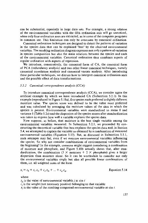
can be substantial, especially in large data sets. For example, a strong relationof the environmental variables with the fifth ordination axis will go unnoticed,when only four ordination axes are extracted, as in some of the computer programsin common use. This limitation can only be overcome by canonical ordination.

Canonical ordination techniques are designed to detect the patterns of variationin the species data that can be explained 'best' by the observed environmentalvariables. The resulting ordination diagram expresses not only a pattern of variationin species composition but also the main relations between the species and eachof the environmental variables. Canonical ordination thus combines aspects ofregular ordination with aspects of regression.

We introduce, consecutively, the canonical form of CA, the canonical formof PCA (redundancy analysis) and two other linear canonical techniques, namelycanonical correlation analysis and canonical variate analysis. After introducingthese particular techniques, we discuss how to interpret canonical ordination axesand the possible effect of data transformations.

5.5.2 Canonical correspondence analysis (CCA)

To introduce canonical correspondence analysis (CCA), we consider again theartificial example by which we have introduced CA (Subsection 5.2.1). In thisexample (reproduced in Figure 5.18a), five species each preferred a slightly differentmoisture value. The species score was defined to be the value most preferredand was calculated by averaging the moisture values of the sites in which thespecies is present. Environmental variables were standardized to mean 0 andvariance 1 (Table 5.2c) and the dispersion of the species scores after standardizationwas taken to express how well a variable explains the species data.

Now suppose, as before, that moisture is the best single variable among theenvironmental variables measured. In Subsection 5.2.1, we proceeded by con-structing the theoretical variable that best explains the species data and, in Section5.4, we attempted to explain the variable so obtained by a combination of measuredenvironmental variables (Equation 5.13). But, as discussed in Subsection 5.5.1,such attempts may fail, even if we measure environmental variables influencingthe species. So why not consider combinations of environmental variables fromthe beginning? In the example, someone might suggest considering a combinationof moisture and phosphate, and Figure 5.18b actually shows that, after stan-dardization, the combination (3 X moisture + 2 X phosphate) gives a largerdispersion than moisture alone. So it can be worthwhile to consider not onlythe environmental variables singly but also all possible linear combinations ofthem, i.e. all weighted sums of the form

Xj = c0 + c, zu + c2 z2i + ... + cq zqi Equation 5.14

whereZji is the value of environmental variable j at site /Cj is the weight (not necessary positive) belonging to that variableJC, is the value of the resulting compound environmental variable at site /.

137

A B C D EI moisture

I I I | * 3x moisture+A B C D E 2x phosphate

J I best 1inearn [; combination

Figure 5.18 Artificial example of unimodal response curves of five species (A-E) with respectto standardized environmental variables showing different degrees of separation of the speciescurves, a: Moisture, b: Linear combination of moisture and phosphate, chosen a priori,c: Best linear combination of environmental variables, chosen by CCA. Sites are shownas dots, at y = 1 if Species D is present and at y - 0 if Species D is absent.

CCA is now the technique that selects the linear combination of environmentalvariables that maximizes the dispersion of the species scores (Figure 5.18c; terBraak 1987a). In other words, CCA chooses the best weights (cy) for theenvironmental variables. This gives the first CCA axis.

The second and further CCA axes also select linear combinations of envir-onmental variables that maximize the dispersion of the species scores, but subjectto the constraint of being uncorrelated with previous CCA axes (Subsection 5.2.1).As many axes can be extracted as there are environmental variables.

CA also maximizes the dispersion of the species scores, though irrespectiveof any environmental variable; that is, CA assigns scores (x,) to sites such thatthe dispersion is absolutely maximum (Subsection 5.2.1). CCA is therefore'restricted correspondence analysis' in the sense that the site scores are restrictedto be a linear combination of measured environmental variables (Equation 5.14).By incorporating this restriction in the two-way weighted averaging algorithm

138

of CA (Table 5.2), we obtain an algorithm for CCA. More precisely, in eachiteration cycle, a multiple regression must be carried out of the site scores obtainedin Step 3 on the environmental variables (for technical reasons with y+i/y++ assite weights). The fitted values of this regression are by definition a linearcombination of the environmental variables (Equation 5.14) and are thus the newsite scores to continue with in Step 4 of Table 5.2a. As in CA, the scores stabilizeafter several iterations and the resulting scores constitute an ordination axis ofCCA. The corresponding eigenvalue actually equals the (maximized) dispersionof the species scores along the axis. The eigenvalues in CCA are usually smallerthan those in CA because of the restrictions imposed on the site scores in CCA.

The parameters of the final regression in the iteration process are the best weights,also called canonical coefficients, and the multiple correlation of this regressionis called the species-environment correlation. This is the correlation between thesite scores that are weighted averages of the species scores and the site scoresthat are a linear combination of the environmental variables. The species-en-vironment correlation is a measure of the association between species andenvironment, but not an ideal one; axes with small eigenvalues may havemisleadingly high species-environment correlations. The importance of the as-sociation is expressed better by the eigenvalue because the eigenvalue measureshow much variation in the species data is explained by the axis and, hence, bythe environmental variables.

CCA is restricted correspondence analysis but the restrictions become less strictthe more environmental variables are included in the analysis. If q ^ n - 1, thenthere are actually no restrictions any more; CCA is then simply CA. The archeffect may therefore crop up in CCA, as it does in CA (Gauch 1982). The methodof detrending (Hill & Gauch 1980) can be used to remove the arch and is availablein the computer program CANOCO (ter Braak 1987b). But in CCA, the archcan be removed more elegantly by dropping superfluous environmental variables.Variables that are highly correlated with the arched axis (often the second axis)are most likely to be superfluous. So a CCA with the superfluous variables excludeddoes not need detrending.

In Subsection 5.2.7, we saw that CA approximated the maximum likelihoodsolution of Gaussian ordination when Conditions A1-A4 hold true. If we changethe Gaussian ordination model by stating that the site scores must be a linearcombination of the environmental variables, the maximum likelihood solutionof the model so obtained is again approximated by CCA when these conditionshold true (ter Braak 1986a). The data on species composition are thus explainedby CCA through a Gaussian response model in which the explanatory variableis a linear combination of the environmental variables. Furthermore, tests of realdata showed that CCA is extremely robust when these assumptions do not hold.The vital assumption is that the response model is unimodal. For a simpler modelwhere relations are monotonic, the results can still be expected to be adequatein a qualitative sense, but for more complex models the method breaks down.

As an example, we use the Dune Meadow Data, which concerns the impactof agricultural use on vegetation in dune meadows on the Island of Terschelling(the Netherlands). The data set consists of 20 releves, 30 plant species (Table

139

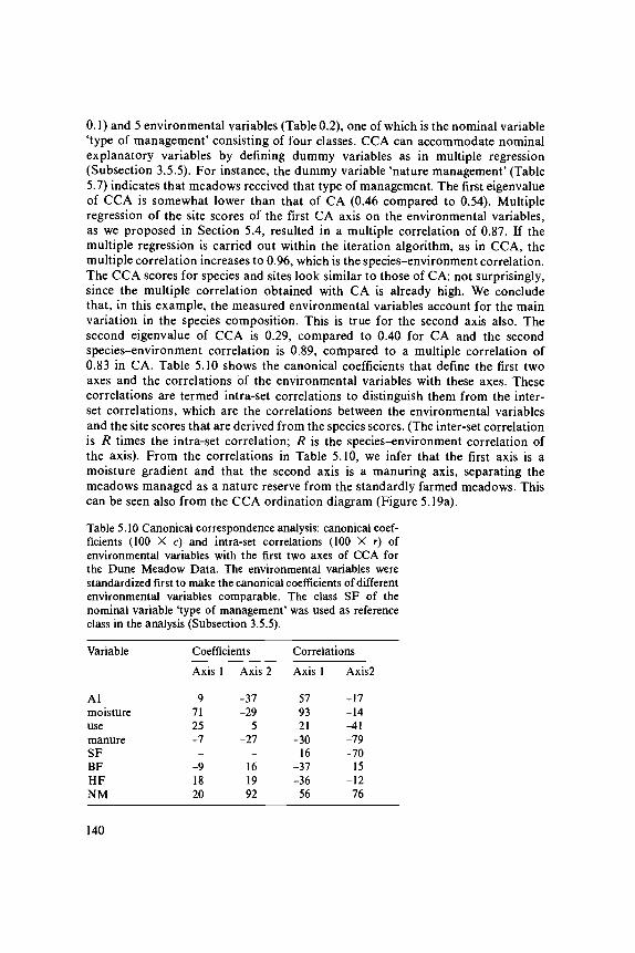
0.1) and 5 environmental variables (Table 0.2), one of which is the nominal variable'type of management' consisting of four classes. CCA can accommodate nominalexplanatory variables by defining dummy variables as in multiple regression(Subsection 3.5.5). For instance, the dummy variable 'nature management' (Table5.7) indicates that meadows received that type of management. The first eigenvalueof CCA is somewhat lower than that of CA (0.46 compared to 0.54). Multipleregression of the site scores of the first CA axis on the environmental variables,as we proposed in Section 5.4, resulted in a multiple correlation of 0.87. If themultiple regression is carried out within the iteration algorithm, as in CCA, themultiple correlation increases to 0.96, which is the species-environment correlation.The CCA scores for species and sites look similar to those of CA: not surprisingly,since the multiple correlation obtained with CA is already high. We concludethat, in this example, the measured environmental variables account for the mainvariation in the species composition. This is true for the second axis also. Thesecond eigenvalue of CCA is 0.29, compared to 0.40 for CA and the secondspecies-environment correlation is 0.89, compared to a multiple correlation of0.83 in CA. Table 5.10 shows the canonical coefficients that define the first twoaxes and the correlations of the environmental variables with these axes. Thesecorrelations are termed intra-set correlations to distinguish them from the inter-set correlations, which are the correlations between the environmental variablesand the site scores that are derived from the species scores. (The inter-set correlationis R times the intra-set correlation; R is the species-environment correlation ofthe axis). From the correlations in Table 5.10, we infer that the first axis is amoisture gradient and that the second axis is a manuring axis, separating themeadows managed as a nature reserve from the standardly farmed meadows. Thiscan be seen also from the CCA ordination diagram (Figure 5.19a).

Table 5.10 Canonical correspondence analysis: canonical coef-ficients (100 X c) and intra-set correlations (100 X r) ofenvironmental variables with the first two axes of CCA forthe Dune Meadow Data. The environmental variables werestandardized first to make the canonical coefficients of differentenvironmental variables comparable. The class SF of thenominal variable 'type of management' was used as referenceclass in the analysis (Subsection 3.5.5).

Variable

AlmoistureusemanureSFBFHFNM

CoefficientsAxis 1

97125-7-

-91820

I Axis 2

-37-29

5-27

-161992

CorrelationsAxis 1

579321

-3016

-37-3656

Axis2

-17-14-41-79-70

15-1276

140

The species and sites are positioned as points in the CCA diagram as in CAand their joint interpretation is also as in CA; sites with a high value of a speciestend to be close to the point for that species (Subsection 5.2.5). The environmentalvariables are represented by arrows and can be interpreted in conjunction withthe species points as follows. Each arrow determines an axis in the diagram andthe species points must be projected onto this axis. As an example, the pointsof a few species are projected on to the axis for manuring in Figure 5.19b. Theorder of the projection points now corresponds approximately to the rankingof the weighted averages of the species with respect to amount of manure. Theweighted average indicates the 'position' of a species curve along an environmentalvariable (Figure 5.18a) and thus the projection point of a species also indicatesthis position, though approximately. Thus Cirsium arvense, Alopecurus genicu-latus, Elymus repens and Poa trivialis mainly occur in these data in the highlymanured meadows, Agrostis stolonifera and Trifolium repens in moderatelymanured meadows and Ranunculus flammula and Anthoxanthum odoratum inmeadows with little manuring. One can interpret the other arrows in a similarway. From Figure 5.19a, one can see at a glance which species occur mainlyin wetter conditions (those on the right of the diagram) and which prefer drierconditions (those on the left of the diagram).

The joint plot of species points and environmental arrows is actually a biplotthat approximates the weighted averages of each of the species with respect toeach of the environmental variables. The rules for quantitative interpretation ofthe CCA biplot are the same as for the PCA biplot described in Subsection 5.3.4.In the diagram, the weighted averages are approximated as deviations from thegrand mean of each environmental variable; the grand mean is represented bythe origin (centroid) of the plot. A second useful rule to interpret the diagramis therefore that the inferred weighted average is higher than average if the projectionpoint lies on the same side of the origin as the head of an arrow and is lowerthan average if the origin lies between the projection point and the head of anarrow. As in Subsection 5.3.2, a measure of goodness of fit is (kl + X2)/(sumof all eigenvalues), which expresses the fraction of variance of the weighted averagesaccounted for by the diagram. In the example, Figure 5.19a accounts for 65%of the variance of the weighted averages. (The sum of all canonical eigenvaluesis 1.177.)

The positions of the heads of the arrows depend on the eigenvalues and onthe intra-set correlations. In Hill's scaling (Subsection 5.2.2), the coordinate ofthe head of the arrow for an environmental variable on axis s is rjs\J\S {\ - Xs), with rjs the intra-set correlation of environmental variable j withaxis s and Xs is the eigenvalue of axis s. The construction of biplots for detrendedcanonical correspondence analysis is described by ter Braak (1986a). Environmentalvariables with long arrows are more strongly correlated with the ordination axesthan those with short arrows, and therefore more closely related to the patternof variation in species composition shown in the ordination diagram.

Classes of nominal environmental variables can also be represented by arrows(ter Braak 1986a). The projection of a species on such an arrow approximatesthe fraction of the total abundance of that species that is achieved at sites of

141

Vic l a t «

Ant odo«

2.0-

Hyp radAir pra Sal rep Emp nig

Pla lan«

Ach mi l*

Tr i praBel per.

-0.5X6 -

5x v 7 BF

-2.0 • . . P o a

Bro hor Lol per 2*

Rum ace*

Ely rep .

Poa t r i

Cir arv •

- Pot pal

• Cal cus

x20

14Ran f1 a

15X 0.5 c scaleJun art*2.0 u scale

moisture -Ele pal

• Agr sto

•Jun buf

-2.0+-0.5 • Alo genChe alb

Figure 5.19 CCA of the Dune Meadow Data, a: Ordination diagram with environmentalvariables represented by arrows. The c scale applies to environmental variables, the u scaleto species and sites. The types of management are also shown by closed squares at thecentroids of the meadows of the corresponding types of management, b: Inferred rankingof the species along the variable amount of manure, based on the biplot interpretationof Part a of this figure.

that class. However it is sometimes more natural to represent each class of anominal variable by a point at the centroid (the weighted average) of the sitesbelonging to that class (Figure 5.19a). Classes consisting of sites with high valuesfor a species are then positioned close to the point of that species. In Figure5.19a, the meadows managed as a nature reserve are seen to lie at the top-rightof the diagram; the meadows of standard farms lie at the bottom.

A second example (from ter Braak 1986a) concerns the presence or absenceof 133 macrophytic species in 125 freshwater ditches in the Netherlands. Thefirst four axes of detrended correspondence analyses (DCA) were poorly related(multiple correlation R < 0.60) to the measured environmental variables, whichwere: electrical conductivity (K), orthophosphate concentration (PHOSPHATE),both transformed to logarithms, chloride ratio (CHLORIDE, the share of chlorideions in K) and soil type (clay, peaty soil, sand). By choosing the axes in the

142

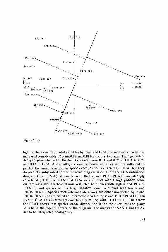
Agr sto

-0.5 ^> » Alo gen

Figure 5.19b

light of these environmental variables by means of CCA, the multiple correlationsincreased considerably, R being 0.82 and 0.81 for the first two axes. The eigenvaluesdropped somewhat - for the first two axes, from 0.34 and 0.25 in DCA to 0.20and 0.13 in CCA. Apparently, the environmental variables are not sufficient topredict the main variation in species composition extracted by DCA, but theydo predict a substantial part of the remaining variation. From the CCA ordinationdiagram (Figure 5.20), it can be seen that K and PHOSPHATE are stronglycorrelated ( > 0.8) with the first CCA axis. Species with a high positive scoreon that axis are therefore almost restricted to ditches with high K and PHOS-PHATE, and species with a large negative score to ditches with low K andPHOSPHATE. Species with intermediate scores are either unaffected by K andPHOSPHATE or restricted to intermediate values of K and PHOSPHATE. Thesecond CCA axis is strongly correlated (r = 0.9) with CHLORIDE. The arrowfor PEAT shows that species whose distribution is the most restricted to peatysoils lie in the top-left corner of the diagram. The arrows for SAND and CLAYare to be interpreted analogously.

143

• Meny trif

Nymp alba«Ranu flam

Pote pal.Ranu ling

peat

Schi gela

Pota acut

Pota per f . •

Call obti

Call hamu*

Ranu aqua

Pota c r i s

Vero anag*

phosphate

Cera subm

•Vero cate

• Tr ib bomb

•Bide t r i p

Pota dec»

Figure 5.20 CCA ordination diagram of the ditch vegetation data (sites are not shown).

5.5.3 Redundancy analysis (RDA)

Redundancy analysis (RDA) is the canonical form of PCA and was inventedby Rao (1964). RDA has so far been neglected by ecologists, but appears attractivewhen used in combination with PCA.

As in PCA (Subsection 5.3.1), we attempt to explain the data of all speciesby fitting a separate straight line to the data of each species. As a measure ofhow badly a particular environmental variable explains the species data, we takethe total residual sum of squares, as in PCA (Figure 5.11). The best environmentalvariable is then the one that gives the smallest total residual sum of squares.From this, we can derive a canonical ordination technique, as in Subsection 5.5.2,by considering also linear combinations of environmental variables. RDA is thetechnique selecting the linear combination of environmental variables that givesthe smallest total residual sum of squares.

PCA also minimizes the total residual sum of squares, but it does so withoutlooking at the environmental variables (Subsection 5.3.1). We can obtain the RDAaxes by extending the algorithm of PCA (Table 5.6) in a similar fashion to how

144

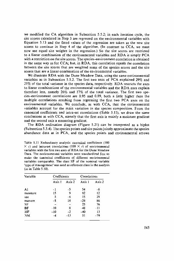
we modified the CA algorithm in Subsection 5.5.2; in each iteration cycle, thesite scores calculated in Step 3 are regressed on the environmental variables withEquation 5.13 and the fitted values of the regression are taken as the new sitescores to continue in Step 4 of the algorithm. (In contrast to CCA, we mustnow use equal site weights in the regression.) So the site scores are restrictedto a linear combination of the environmental variables and RDA is simply PCAwith a restriction on the site scores. The species-environment correlation is obtainedin the same way as for CCA; but, in RDA, this correlation equals the correlationbetween the site scores that are weighted sums of the species scores and the sitescores that are a linear combination of the environmental variables.

We illustrate RDA with the Dune Meadow Data, using the same environmentalvariables as in Subsection 5.5.2. The first two axes of PCA explained 29% and21% of the total variance in the species data, respectively. RDA restricts the axesto linear combinations of the environmental variables and the RDA axes explaintherefore less, namely 26% and 17% of the total variance. The first two spe-cies-environment correlations are 0.95 and 0.89, both a little higher than themultiple correlations resulting from regressing the first two PCA axes on theenvironmental variables. We conclude, as with CCA, that the environmentalvariables account for the main variation in the species composition. From thecanonical coefficients and intra-set correlations (Table 5.11), we draw the sameconclusions as with CCA, namely that the first axis is mainly a moisture gradientand the second axis a manuring gradient.

The RDA ordination diagram (Figure 5.21) can be interpreted as a biplot(Subsection 5.3.4). The species points and site points jointly approximate the speciesabundance data as in PCA, and the species points and environmental arrows

Table 5.11 Redundancy analysis: canonical coefficients (100X c) and intra-set correlations (100 X r) of environmentalvariables with the first two axes of RDA for the Dune MeadowData. The environmental variables were standardized first tomake the canonical coefficients of different environmentalvariables comparable. The class SF of the nominal variable'type of management' was used as reference class in the analysis(as in Table 5.10).

Variable

AlmoistureusemanureSFBFHFNM

Coefficients

Axis 1

-1155

-8-

-10-10

-4

Axis 2

_59

-616-0

-2-13

Correlations

Axis 1

549215

-2625

-48-40

51

Axis 2

-612298676

-1113

-79

145

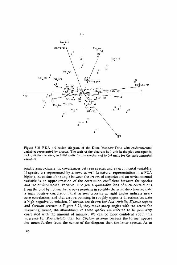
Agr sto

Emp nig\» • Cal cus#\fot palAir pra

Figure 5.21 RDA ordination diagram of the Dune Meadow Data with environmentalvariables represented by arrows. The scale of the diagram is: 1 unit in the plot correspondsto 1 unit for the sites, to 0.067 units for the species and to 0.4 units for the environmentalvariables.

jointly approximate the covariances between species and environmental variables.If species are represented by arrows as well (a natural representation in a PCAbiplot), the cosine of the angle between the arrows of a species and an environmentalvariable is an approximation of the correlation coefficient between the speciesand the environmental variable. One gets a qualitative idea of such correlationsfrom the plot by noting that arrows pointing in roughly the same direction indicatea high positive correlation, that arrows crossing at right angles indicate near-zero correlation, and that arrows pointing in roughly opposite directions indicatea high negative correlation. If arrows are drawn for Poa trivialis, Elymus repensand Cirsium arvense in Figure 5.21, they make sharp angles with the arrow formanuring; hence, the abundances of these species are inferred to be positivelycorrelated with the amount of manure. We can be more confident about thisinference for Poa trivialis than for Cirsium arvense because the former specieslies much further from the centre of the diagram than the latter species. As in

146

PCA, species at the centre of the diagram are often not very well representedand inferences from the diagram about their abundances and correlations areimprecise. From Figure 5.21, we infer also that, for instance, Salix repens,Hypochaeris radicata and Air a praecox are negatively correlated with the amountof manure.

A measure of goodness of fit of the biplot of species and environmental variablesis (\x + )i2)/(sum of all eigenvalues), which expresses the fraction of varianceof all covariances between species and environment accounted for by the diagram.For the example, Figure 5.21 accounts for 71% of this variance.

The scaling of Figure 5.21 conforms to that of the Euclidean distance biplot(Subsection 5.3.4): the sum of squares of the species scores is unity and site pointsare obtained by weighted summation of species scores. The positions of the headsof arrows of the environmental variables depend on the intra-set correlations (Table5.11) and the eigenvalues. With this scaling, the coordinate of the head of thearrow for an environmental variable on axis s must be rjs y(ks/ri) where rjs isthe intra-set correlation of environmental variable j with axis s, n is the numberof sites, and Xs the eigenvalue of axis s. The diagram scaled in this way givesnot only a least-squares approximation of the covariances between species andenvironment, but also approximations of the (centred) abundances values, of theEuclidean Distances among the sites as based on the species data (Equation 5.15),and of covariances among the environmental variables, though the latter twoapproximations are not least-squares approximations. Other types of scaling arepossible (ter Braak 1987b).

5.5.4 Canonical correlation analysis (COR)

The species-environment correlation was a by-product in CCA and RDA, butis central in canonical correlation analysis (COR). The idea of COR is to choosecoefficients (scores) for species and coefficients for environmental variables soas to maximize the species-environment correlation. In COR, the species-envir-onment correlation is defined as in RDA, as the correlation between site scores(xf) that are weighted sums of species scores: (x(* = I.k bk yki) and site scores(*,-) that are a linear combination of the environmental variables (*, = c0 +I ; Cj Zji). An algorithm to obtain the COR axes is given in Table 5.12. The resultingspecies-environment correlation is termed the canonical correlation, and is actuallythe squareroot of the first eigenvalue of COR. Step 2 of the algorithm makesthe difference from RDA: in RDA, the species scores are simply a weighted sumof the site scores, whereas in COR the species scores are parameters estimatedby a multiple regression of the site scores on the species variables. This regressionhas the practical consequence that, in COR, the number of species must be smallerthan the number of sites. It can be shown that the restriction on the numberof species is even stronger than that: the number of species plus the numberof environmental variables must be smaller than the number of sites. Thisrequirement is not met in our Dune Meadow Data and is generally a nuisancein ecological research. By contrast, RDA and CCA set no upper limit to thenumber of species that can be analysed. Examples of COR can be found in Gittins

147

Table 5.12 An iteration algorithm for canonical correlation analysis (COR).

Step 1. Start with arbitrary initial site scores (*,), not all equal to zero.Step 2. Calculate species scores by multiple regression of the site scores on the species variables.

The species scores (bk) are the parameter estimates of this regression.Step 3. Calculate new site scores (x*) by weighted summation of the species scores (Equation 5.9).

The site scores in fact equal the fitted values of the multiple regression of Step 2.Step 4. Calculate coefficients for the environmental variables by multiple regression of the site

scores (x*) on the environmental variables. The coefficients {cj) are the parameter estimatesof this regression.

Step 5. Calculate new site scores (x,) by weighted summation of the coefficients of the environmentalvariables, i.e. by xt = I,jL\ Cj zir The site scores in fact equal the fitted values of the multipleregression of Step 4.

Step 6. For second and higher axes, orthogonalize the site scores (JC,) as in Table 5.6.Step 7. Standardize the site scores (x,) as in Table 5.6.Step 8. Stop on convergence, i.e. when the new site scores are sufficiently close to the site scores

of the previous cycle of the iteration process; ELSE go to Step 2.

(1985). COR allows a biplot to be made, from which the approximate covariancesbetween species and environmental variables can be derived in the same way asin RDA (Subsection 5.5.3). The construction of the COR biplot is given inSubsection 5.9.3.

In our introduction to COR, species and environmental variables enter the analysisin a symmetric way (Table 5.12). Tso (1981) presented an asymmetric approachin which the environmental variables explain the species data. In this approachCOR is very similar to RDA, but differs from it in the assumptions about theerror part of the model (Equations 5.10 and 5.14): uncorrelated errors with equalvariance in RDA and correlated normal errors in COR. The residual correlationsbetween errors are therefore additional parameters in COR. When the numberof species is large, there are so many of them that they cannot be estimated reliablyfrom data from few sites. This causes practical problems with COR that are absentin RDA and CCA.

5.5.5 Canonical variate analysis (CVA)

Canonical variate analysis (CVA) belongs to the classical linear multivariatetechniques along with PCA and COR. CVA is also termed linear discriminantanalysis.

If sites are classified into classes or clusters, we may wish to know how thespecies composition differs among sites of different classes. If we have recordedthe abundance values of a single species only, this question reduces to how muchthe abundance of the species differs between classes, a question studied in Subsection3.2.1 by analysis of variance. If there are more species, we may wish to combinethe abundance values of the species to make the differences between classes clearerthan is possible on the basis of the abundance values of a single species. CVAdoes so by seeking a weighted sum of the species abundances; however not one

148

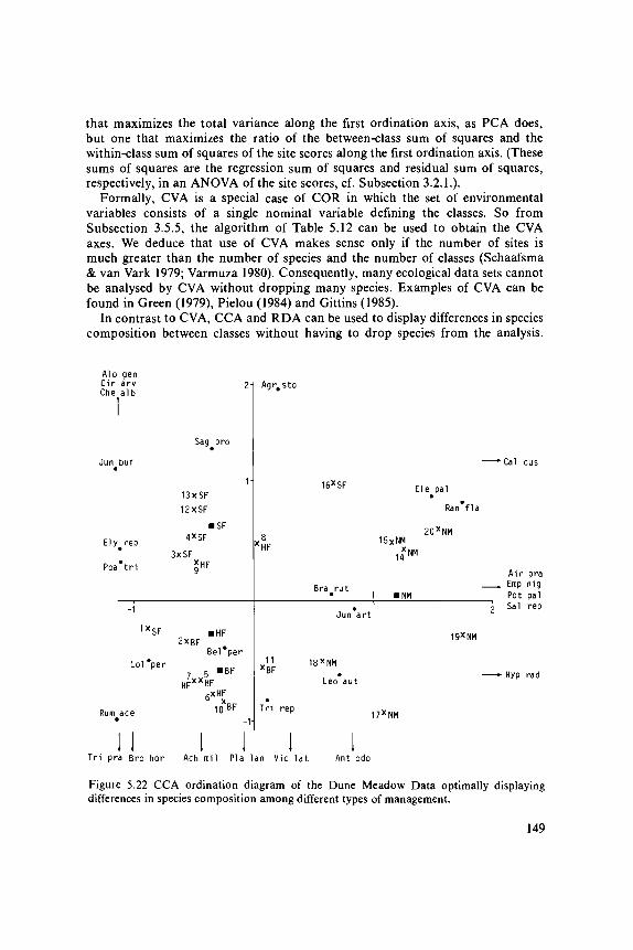
that maximizes the total variance along the first ordination axis, as PCA does,but one that maximizes the ratio of the between-class sum of squares and thewithin-class sum of squares of the site scores along the first ordination axis. (Thesesums of squares are the regression sum of squares and residual sum of squares,respectively, in an ANOVA of the site scores, cf. Subsection 3.2.1.).

Formally, CVA is a special case of COR in which the set of environmentalvariables consists of a single nominal variable defining the classes. So fromSubsection 3.5.5, the algorithm of Table 5.12 can be used to obtain the CVAaxes. We deduce that use of CVA makes sense only if the number of sites ismuch greater than the number of species and the number of classes (Schaafsma& van Vark 1979; Varmuza 1980). Consequently, many ecological data sets cannotbe analysed by CVA without dropping many species. Examples of CVA can befound in Green (1979), Pielou (1984) and Gittins (1985).

In contrast to CVA, CCA and RDA can be used to display differences in speciescomposition between classes without having to drop species from the analysis.

Alo genCiurChe

Jun•

Ely

Poa

Rum

arvalb

buf

rep

•tri

-1

1 XSF

Lol *per

ace

Sag pro

13XSF

12XSF

• SF4*SF

3xSFXHF

2XBFBel 'per

7 5 " B F

HFXXHF6xH

xF

1 0 BF

2-

1-

-1 -

Agr#sto

*BF

Tr i rep

16XSF

15XNM

1 4XN

Bra r u t• 1 BNM

Jun a r t

18*NM

Leo aut

17XNM

Ele pal

Ran*fla

20xNM

M

19XNM

"Cal cus

Air praEmp nigPot pal

J Sal rep

- Hyp rad

T r i pra Bro hor Ach mil Pla Ian Vic l a t Ant odo

Figure 5.22 CCA ordination diagram of the Dune Meadow Data optimally displayingdifferences in species composition among different types of management.

149

For this, we must code classes as dummy environmental variables, as in Subsection3.5.5. Such an analysis by CCA is equivalent to the analysis of concentrationproposed by Feoli & Orloci (1979). As an example, Figure 5.22 displays thedifferences in vegetation composition between the meadows receiving differenttypes of management in our Dune Meadow Data. The first axis (A,, = 0.32) isseen to separate the meadows receiving nature management from the remainingmeadows and second axis (k2 = 0.18) separates the meadows managed by standardfarming from those managed by hobby farming and biological farming, althoughthe separations are not perfect. The species displayed on the right side of thediagram occur mainly in the meadows receiving nature management and thoseon the upper left in the meadows managed by standard farming, and so on. Figure5.22 displays almost the same information as Figure 5.19a, as can be seen byjoining Site Points 16 and 18 in both diagrams. Moisture and manuring arepresumably the major factors bringing about vegetation differences between typesof management.

5.5.6 Interpreting canonical axes

To interpret the ordination axes, one can use the canonical coefficients andthe intra-set correlations. The canonical coefficients define the ordination axesas linear combinations of the environmental variables by means of Equation 5.14and the intra-set correlations are the correlation coefficients between the envir-onmental variables and these ordination axes. As before, we assume that theenvironmental variables have been standardized to a mean of 0 and a varianceof 1 before the analysis. This standardization removes arbitrariness in the unitsof measurement of the environmental variables and makes the canonical coefficientscomparable among each other, but does not influence other aspects of the analysis.

By looking at the signs and relative magnitudes of the intra-set correlationsand of the canonical coefficients standardized in this way, we may infer the relativeimportance of each environmental variable for prediction of species composition.The canonical coefficients give the same information as the intra-set correlations,if the environmental variables are mutually uncorrelated, but may provide ratherdifferent information if the environmental variables are correlated among oneanother, as they usually are in field data. Both a canonical coefficient and anintra-set correlation relate to the rate of change in species composition by changingthe corresponding environmental variable. However it is assumed that otherenvironmental variables are being held constant in the former case, whereas theother environmental variables are assumed to covary with that one environmentalvariable in the particular way they do in the data set in the latter case. If theenvironmental variables are strongly correlated with one another, for examplesimply because the number of environmental variables approaches the numberof sites, the effects of different environmental variables on the species compositioncannot be singled out and, consequently, the canonical coefficients will be unstable.This is the multicollinearity problem discussed in the context of multiple regressionin Subsection 3.5.3. The algorithms to obtain the canonical axes show that canonicalcoefficients are actually coefficients of a multiple regression (Subsection 5.5.2),

150

so both suffer identical problems. If the multicollinearity problem arises (theprogram CANOCO (ter Braak 1987b) provides statistics to help detecting it),one should abstain from attempts to interpret the canonical coefficients. But theintra-set correlations do not suffer from this problem. They are more like simplecorrelation coefficients. They can still be interpreted. One can also removeenvironmental variables from the analysis, keeping at least one variable per setof strongly correlated environmental variables. Then, the eigenvalues and spe-cies-environment correlations will usually only decrease slightly. If the eigenvaluesand species-environment correlations drop considerably, one has removed toomany (or the wrong) variables.

Their algorithms indicate that COR and CVA are hampered also by strongcorrelations among species, whereas CCA and RDA are not. So in CCA andRDA, the number of species is allowed to exceed the number of sites.

5.5.7 Data transformation

As in CA and PCA, any kind of transformation of the species abundancesmay affect the results of CCA and RDA. We refer to Subsections 5.2.2 and 5.3.5for recommendations about this. The results of COR and CVA are affected bynon-linear transformations of the species data, but not by linear transformations.Canonical ordination techniques are not influenced by linear transformations ofthe environmental variables, but non-linear transformation of environmentalvariables can be considered if there is some reason to do so. Prior knowledgeabout the possible impact of the environmental variables on species compositionmay suggest particular non-linear transformations and particular non-linearcombinations, i.e. environmental scalars in the sense of Loucks (1962) and Austinet al. (1984). The use of environmental scalars can also circumvent the multi-collinearity problem described in Subsection 5.5.6.

5.6 Multidimensional scaling

In Section 5.1, ordination was defined as a method that arranges site pointsin the best possible way in a continuum such that points that are close togethercorrespond to sites that are similar in species composition, and points which arefar apart correspond to sites that are dissimilar. A particular ordination techniqueis obtained by further specifying what 'similar' means and what 'best' is. Thedefinition suggests that we choose a measure of (dis)similarity between sites(Subsection 6.2.2), replace the original species composition data by a matrix ofdissimilarity values between sites and work further from the dissimilarity matrixto obtain an ordination diagram. This final step is termed multidimensional scaling.

In general, it is not possible to arrange sites such that the mutual distancesbetween the sites in the ordination diagram are equal to the calculated dissimilarityvalues. Therefore a measure is needed that expresses in a single number howwell or how badly the distances in the ordination diagram correspond to thedissimilarity values. Such a measure is termed a loss function or a stress function.In metric ordination techniques such as CA and PCA, the loss function depends

151

on the actual numerical values of the dissimilarities, whereas, in non-metrictechniques, the loss function depends only on the rank order of the dissimilarities.

In CA and PCA, one need not calculate a matrix of dissimilarity values first,yet those techniques use particular measures of dissimilarity. In CA, the impliedmeasure of dissimilarity is the chi-squared distance and, in PCA, the EuclideanDistance, as follows immediately from Subsection 5.3.3. The chi-square distanced^ between site / and site j is defined as

5 / = y++ I^xiyuly+i - ykjly+j)2 lyk+ Equation 5.15

and the Euclidean Distance 5,y between these sites is

V = S*=> Ofc - V 2 Equation 5.16

The chi-squared distance involves proportional differences in abundances of speciesbetween sites, whereas the Euclidean Distance involves absolute differences.Differences in site and species totals are therefore less influential in CA thanin PCA, unless a data transformation is used in PCA to correct for this effect.

A simple metric technique for multidimensional scaling is principal coordinateanalysis (PCO), also called classical scaling (Gower 1966; Pielou 1977, p.290-395). PCO is based on PCA, but is more general than PCA, in that other measuresof dissimilarity may be used than Euclidean Distance. In PCO, the dissimilarityvalues by are transformed into similarity values by the equation

ctj= -0.5 (5? - %/n - b2

+jln + 52++/«2) Equation 5.17

where the index + denotes a sum of squared dissimilarities. The matrix withelements ctj is then subjected to the Q-mode algorithm of PCA (Subsection 5.3.6).If the original dissimilarities were computed as Euclidean Distances, PCO isidentical to species-centred PCA calculated by the Q-mode algorithm.

In most techniques for (non-metric) multidimensional scaling, we must specifya priori the number of ordination axes and supply an initial ordination of sites.The technique then attempts to modify the ordination iteratively to minimizethe stress. In contrast to the iterative algorithms for CA, PCA and PCO, differentinitial ordinations may lead to different results, because of local minima in thestress function (Subsection 5.2.7); hence, we must supply a 'good' initial ordinationor try a series of initial ordinations. From such trials, we then select the ordinationwith minimum stress.

The best known technique for non-metric multidimensional scaling is ascribedto Shepard (1962) and Kruskal (1964). The stress function, which is minimizedin their technique, is based on the Shepard diagram. This is a scatter diagramof the dissimilarities (5,y) calculated from the species data against the distancesdy between the sites in the ordination diagram.

The ordination fits perfectly (stress = 0), if the dissimilarities are monotonicwith the distances, i.e. if the points in the Shepard plot lie on a monotonicallyincreasing curve. If they do not, we can fit a monotonic curve through the points

152

by least-squares. This is called monotonic or isotonic regression (Barlow et al.1972). We then use as stress, a function of the residual sum of squares (for example,Kruskal's stress formula 1, which is the residual sum of squares divided by thetotal sum of squared distances). The algorithm to seek the ordination that minimizesthe stress proceeds further as described above. Note that the method can workequally well with similarities, the only modifications being that a monotonicallydecreasing curve is fitted in the Shepard diagram. There are two methods to dealwith equal dissimilarity values (ties). In the primary approach to ties, thecorresponding fitted distances need not be equal, whereas they must be equalin the secondary approach. The primary approach to ties is recommended, becauseequal dissimilarity values do not necessarily imply equal habitat differences, inpart*cular if the equalities arise between pairs of sites that have no species incommon (Prentice 1977).

The Shepard-Kruskal method is based on the rank order of all dissimilarities.But calculated dissimilarities may not be comparable in different parts of a gradient,for example if there is a trend in species richness. This potential problem canbe overcome by making a separate Shepard diagram for each site, in which weplot the dissimilarities and distances between the particular site and all remainingsites. Each Shepard diagram the distances leads to a stress value and the totalstress is taken to be a combination of the separate stress values. This is the localnon-metric technique proposed by Sibson (1972). Prentice (1977; 1980) advocateda particular similarity coefficient for use in Sibson's technique. This coefficient is

stj — Ij. minO^,,^) Equation 5.18

Kendall (1971) proved that this coefficient contains all the information requiredto reconstruct the order of sites when abundances of species follow arbitraryunimodal response curves.

5.7 Evaluation of direct gradient and indirect gradient analysis techniques

Table 5.13 summarizes the techniques described in Chapters 3, 4 and 5 by typeof response model and types of variables. We can classify response models aslinear and non-linear. Each linear technique (from multiple regression to COR)has non-linear counterparts. A non-linear model that has special relevance incommunity ecology is the unimodal model. In principle, unimodal models canbe fitted to data by the general methods used for non-linear models (in particularby maximum likelihood methods). For regression analysis, these methods areavailable (GLM, Chapter 3) but, in ordination, they are not so readily availableand tend to require excessive computing. Therefore we have also introduced muchsimpler methods for analysing data for which unimodal models are appropriate.These simple methods start from the idea that the optima of species responsecurves can be estimated roughly by weighted averaging and we have shown (Section3.7) that under particular conditions the estimates are actually quite good. Thisidea resulted in CA, DCA and CCA.

Multidimensional scaling is left out of Table 5.13, because it is unclear what

153

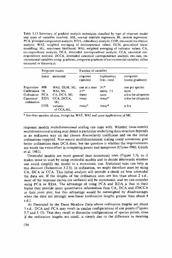
Table 5.13 Summary of gradient analysis techniques classified by type of response modeland types of variables involved. MR, normal multiple regression; IR, inverse regression;PCA, principal components analysis; RDA, redundancy analysis; COR, canonical correlationanalysis; WAE, weighted averaging of environmental values; GLM, generalized linearmodelling; ML, maximum likelihood; WAI, weighted averaging of indicator values; CA,correspondence analysis; DCA, detrended correspondence analysis; CCA, canonical cor-respondence analysis; DCCA, detrended canonical correspondence analysis; env.vars, en-vironmental variables; comp. gradients, composite gradients of environmental variables, eithermeasured or theoretical.

RegressionCalibrationOrdinationCanonicalordination

Response model

linear

MRIRPCARDA

COR

unimodal

WAE, GLM, MLWAI, MLCA, DCA, MLCCA, DCCA,

MLvariants

of CCA,ML

Number of variables

response(species)

explanatory(env. vars)

one at a time ^ 1 *>\*manymany

many*

rarely >1nonemany*

many*

composite(comp.gradients)

one per speciesnonea few for all speciesa few for all species

a few

* less than number of sites, except for WAE, WAI and some applications of ML.

response models multidimensional scaling can cope with. Whether (non-metric)multidimensional scaling may detect a particular underlying data structure dependsin an unknown way on the chosen dissimilarity coefficient and on the initialordinations supplied. Non-metric multidimensional scaling could sometimes givebetter ordinations than DCA does, but the question is whether the improvementsare worth the extra effort in computing power and manpower (Clymo 1980; Gauchetal. 1981).

Unimodal models are more general than monotonic ones (Figure 3.3), so itmakes sense to start by using unimodal models and to decide afterwards whetherone could simplify the model to a monotonic one. Statistical tests can help inthis decision (Subsection 3.2.3). In ordination, we might therefore start by usingCA, DCA or CCA. This initial analysis will provide a check on how unimodalthe data are. If the lengths of the ordination axes are less than about 2 s.d.,most of the response curves (or surfaces) will be monotonic, and we can considerusing PCA or RDA. The advantage of using PCA and RDA is that in theirbiplot they provide more quantitative information than CA, DCA and (D)CCAin their joint plot, but this advantage would be outweighed by disadvantageswhen the data are strongly non-linear (ordination lengths greater than about 4s.d.).

As illustrated by the Dune Meadow Data whose ordination lengths are about3 s.d., DCA and PCA may result in similar configurations of site points (Figures5.7 and 5.15). That they result in dissimilar configurations of species points, evenif the ordination lengths are small, is simply due to the difference in meaning

154

of the species scores in DCA and PCA (Subsections 5.2.5 and 5.3.5).Table 5.13 also shows the types of variables involved in regression, calibration,

ordination and canonical ordination. We distinguish between response variables,explanatory variables and 'composite' variables, which in community ecologytypically correspond to species presences or abundances, measured environmentalvariables and 'composite gradients', respectively. A composite gradient is eithera linear combination of measured environmental variables or a theoretical variable.Which technique is the appropriate one to use largely depends on the researchpurpose and the type of data available. Ordination and cluster analysis (Chapter6) are the only available techniques when one has no measured environmentaldata. Calibration must be considered if one wants to make inferences about valuesof a particular environmental variable from species data and existing knowledgeof species-environment relations. Regression and canonical ordination are calledfor if one wants to build up and extend the knowledge of species-environmentrelations (Subsections 3.1.1 and 5.1.1).

Whether to use regression or to use canonical ordination depends on whetherit is considered advantageous to analyse all species simultaneously or not. Ina simultaneous analysis by canonical ordination, one implicitly assumes that allspecies are reacting to the same composite gradients of environmental variablesaccording to a common response model. The assumption arises because canonicalordination constructs a few composite gradients for all species. By contrast inregression analysis, a separate composite gradient is constructed for each species.Regression may therefore result in more detailed descriptions and more accuratepredictions of each particular species, at least if sufficient data are available.However ecological data that are collected over a large range of habitat variationrequire non-linear models; building good non-linear models by regression is noteasy, because it requires construction of composite gradients that are non-linearcombinations of environmental variables (Subsection 3.5.4). In CCA, the compositegradients are linear combinations of environmental variables, giving a much simpleranalysis, and the non-linearity enters the model through a unimodal model fora few composite gradients, taken care of in CCA by weighted averaging. Canonicalordination is easier to apply and requires less data than regression. It providesa summary of the species-environment relations. The summary may lack the kindof detail that can in principle be provided by regression; on the other hand, theadvantages of using regression, with its machinery of statistical tests, may belost in practice, through the sheer complexity of non-linear model building andthrough lack of data. Because canonical ordination gives a more global picturethan regression, it may be advantageous to apply canonical ordination in theearly exploratory phase of the analysis of a particular data set and to applyregression in subsequent phases to selected species and environmental variables.

As already shown in the examples in Subsection 5.5.2, canonical ordinationand ordination followed by environmental interpretation can be used fruitfullyin combination. If the results do not differ much, then we know that no importantenvironmental variables have been overlooked in the survey. But note that thoseincluded could merely be correlated with the functionally important ones. A furtherproviso is that the number of environmental variables (q) is small compared to

155

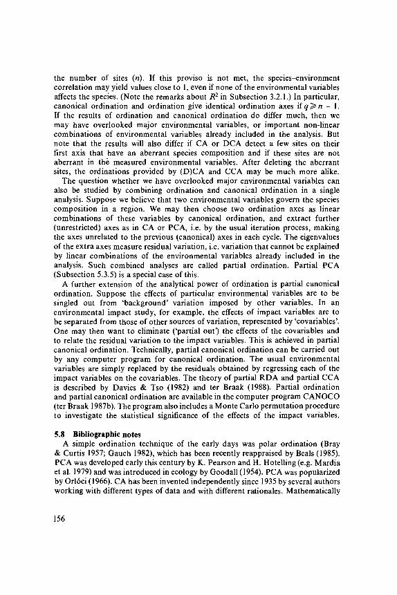
the number of sites (n). If this proviso is not met, the species-environmentcorrelation may yield values close to 1, even if none of the environmental variablesaffects the species. (Note the remarks about R2 in Subsection 3.2.1.) In particular,canonical ordination and ordination give identical ordination axes ifq^n - 1.If the results of ordination and canonical ordination do differ much, then wemay have overlooked major environmental variables, or important non-linearcombinations of environmental variables already included in the analysis. Butnote that the results will also differ if CA or DCA detect a few sites on theirfirst axis that have an aberrant species composition and if these sites are notaberrant in the measured environmental variables. After deleting the aberrantsites, the ordinations provided by (D)CA and CCA may be much more alike.

The question whether we have overlooked major environmental variables canalso be studied by combining ordination and canonical ordination in a singleanalysis. Suppose we believe that two environmental variables govern the speciescomposition in a region. We may then choose two ordination axes as linearcombinations of these variables by canonical ordination, and extract further(unrestricted) axes as in CA or PCA, i.e. by the usual iteration process, makingthe axes unrelated to the previous (canonical) axes in each cycle. The eigenvaluesof the extra axes measure residual variation, i.e. variation that cannot be explainedby linear combinations of the environmental variables already included in theanalysis. Such combined analyses are called partial ordination. Partial PCA(Subsection 5.3.5) is a special case of this.

A further extension of the analytical power of ordination is partial canonicalordination. Suppose the effects of particular environmental variables are to besingled out from 'background' variation imposed by other variables. In anenvironmental impact study, for example, the effects of impact variables are tobe separated from those of other sources of variation, represented by 'covariables'.One may then want to eliminate ('partial out') the effects of the covariables andto relate the residual variation to the impact variables. This is achieved in partialcanonical ordination. Technically, partial canonical ordination can be carried outby any computer program for canonical ordination. The usual environmentalvariables are simply replaced by the residuals obtained by regressing each of theimpact variables on the covariables. The theory of partial RDA and partial CCAis described by Davies & Tso (1982) and ter Braak (1988). Partial ordinationand partial canonical ordination are available in the computer program CANOCO(ter Braak 1987b). The program also includes a Monte Carlo permutation procedureto investigate the statistical significance of the effects of the impact variables.

5.8 Bibliographic notesA simple ordination technique of the early days was polar ordination (Bray

& Curtis 1957; Gauch 1982), which has been recently reappraised by Beals (1985).PCA was developed early this century by K. Pearson and H. Hotelling (e.g. Mardiaet al. 1979) and was introduced in ecology by Goodall (1954). PCA was popularizedby Orloci (1966). CA has been invented independently since 1935 by several authorsworking with different types of data and with different rationales. Mathematically

156

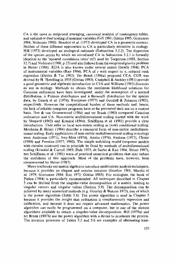
CA is the same as reciprocal averaging, canonical analysis of contingency tables,and optimal or dual scaling of nominal variables (Gifi 1981; Gittins 1985; Greenacre1984; Nishisato 1980). Benzecri et al. (1973) developed CA in a geometric context.Neither of these different approaches to CA is particularly attractive in ecology.Hill (1973) developed an ecological rationale (Subsection 5.2.2). The dispersionof the species scores by which we introduced CA in Subsection 5.2.1 is formallyidentical to the 'squared correlation ratio' (rj2) used by Torgerson (1958, Section12.7) and Nishisato (1980, p.23) and also follows from the reciprocal gravity problemin Heiser (1986). RDA is also known under several names (Israels 1984): PC Aof instrumental variables (Rao 1964), PC A of y with respect to x, reduced rankregression (Davies & Tso 1982). Ter Braak (1986a) proposed CCA. COR wasderived by H. Hotelling in 1935 (Gittins 1985). Cairipbell & Atchley (1981) providea good geometric and algebraic introduction to CVA and Williams (1983) discussesits use in ecology. Methods to obtain the maximum likelihood solutions forGaussian ordination have been investigated, under the assumption of a normaldistribution, a Poisson distribution and a Bernoulli distribution for the speciesdata, by Gauch et al. (1974), Kooijman (1977) and Goodall & Johnson (1982),respectively. However the computational burden of these methods and, hence,the lack of reliable computer programs have so far prevented their use on a routinebasis. Ihm & van Groenewoud (1984) and ter Braak (1985) compared Gaussianordination and CA. Non-metric multidimensional scaling started with the workby Shepard (1962) and Kruskal (1964). Schiffman et al. (1981) provide a clearintroduction. They refer to local non-metric scaling as (row) conditional scaling.Meulman & Heiser (1984) describe a canonical form of non-metric multidimen-sional scaling. Early applications of non-metric multidimensional scaling in ecologywere Anderson (1971), Noy-Meir (1974), Austin (1976), Fasham (1977), Clymo(1980) and Prentice (1977; 1980). The simple unfolding model (response modelswith circular contours) can in principle be fitted by methods of multidimensionalscaling (Kruskal & Carroll 1969; Dale 1975; de Sarbo & Rao 1984; Heiser 1987),but Schiffman et al. (1981) warn of practical numerical problems that may reducethe usefulness of this approach. Most of the problems have, however, beencircumvented by Heiser (1987).

Many textbooks use matrix algebra to introduce multivariate analysis techniques,because it provides an elegant and concise notation (Gordon 1981; Mardia etal. 1979; Greenacre 1984; Rao 1973; Gittins 1985). For ecologists, the book ofPielou (1984) is particularly recommended. All techniques described in Chapter5 can be derived from the singular-value decomposition of a matrix, leading tosingular vectors and singular values (Section 5.9). The decomposition can beachieved by many numerical methods (e.g. Gourlay & Watson 1973), one of whichis the power algorithm (Table 5.6). The power algorithm is used in Chapter 5because it provides the insight that ordination is simultaneously regression andcalibration, and because it does not require advanced mathematics. The poweralgorithm can easily be programmed on a computer, but is one of the slowestalgorithms available to obtain a singular-value decomposition. Hill (1979a) andter Braak (1987b) use the power algorithm with a device to accelerate the process.The iteration processes of Tables 5.2 and 5.6 are examples of alternating least-

157

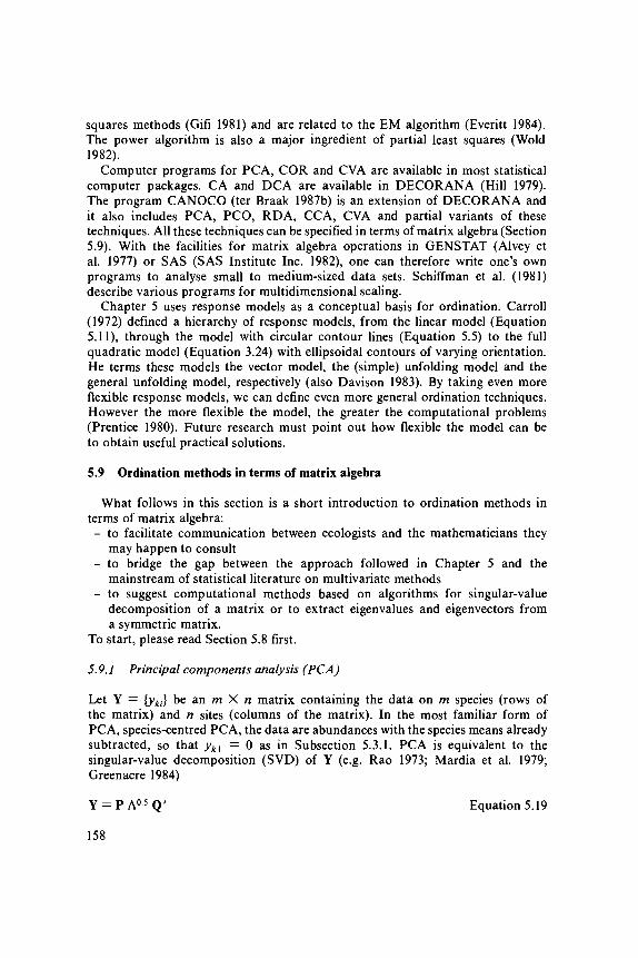
squares methods (Gifi 1981) and are related to the EM algorithm (Everitt 1984).The power algorithm is also a major ingredient of partial least squares (Wold1982).

Computer programs for PCA, COR and CVA are available in most statisticalcomputer packages. CA and DC A are available in DECOR AN A (Hill 1979).The program CANOCO (ter Braak 1987b) is an extension of DECOR AN A andit also includes PCA, PCO, RDA, CCA, CVA and partial variants of thesetechniques. All these techniques can be specified in terms of matrix algebra (Section5.9). With the facilities for matrix algebra operations in GENSTAT (Alvey etal. 1977) or SAS (SAS Institute Inc. 1982), one can therefore write one's ownprograms to analyse small to medium-sized data sets. Schiffman et al. (1981)describe various programs for multidimensional scaling.

Chapter 5 uses response models as a conceptual basis for ordination. Carroll(1972) defined a hierarchy of response models, from the linear model (Equation5.11), through the model with circular contour lines (Equation 5.5) to the fullquadratic model (Equation 3.24) with ellipsoidal contours of varying orientation.He terms these models the vector model, the (simple) unfolding model and thegeneral unfolding model, respectively (also Davison 1983). By taking even moreflexible response models, we can define even more general ordination techniques.However the more flexible the model, the greater the computational problems(Prentice 1980). Future research must point out how flexible the model can beto obtain useful practical solutions.

5.9 Ordination methods in terms of matrix algebra

What follows in this section is a short introduction to ordination methods interms of matrix algebra:

- to facilitate communication between ecologists and the mathematicians theymay happen to consult

- to bridge the gap between the approach followed in Chapter 5 and themainstream of statistical literature on multivariate methods

- to suggest computational methods based on algorithms for singular-valuedecomposition of a matrix or to extract eigenvalues and eigenvectors froma symmetric matrix.

To start, please read Section 5.8 first.

5.9.1 Principal components analysis (PCA)

Let Y = {yki} be an m X n matrix containing the data on m species (rows ofthe matrix) and n sites (columns of the matrix). In the most familiar form ofPCA, species-centred PCA, the data are abundances with the species means alreadysubtracted, so that yk+ = 0 as in Subsection 5.3.1. PCA is equivalent to thesingular-value decomposition (SVD) of Y (e.g. Rao 1973; Mardia et al. 1979;Greenacre 1984)

Y = P A 0 5 Q ' Equation 5.19

158

where P and Q are orthonormal matrices of dimensions m X r and n X r, respectively,with r = min (m,n), i.e. P 'P = I and Q'Q = I, and A is a diagonal matrixwith diagonal elements Xs (s = 1 ... r), which are arranged in order of decreasingmagnitude A,, ̂ X2 ̂ ^3 ̂ ••• ^ 0.

The columns of P and Q contain the singular vectors of Y, and \®-5 is the 5thsingular value of Y. If the 5th column of P is denoted by p5, an m vector, andthe 5th column of Q by q,, an n vector, Equation 5.19 can be written as

Y = l;=1 ^ 0 5 p 5 q / Equation 5.20

The least-squares approximation of Y in Equation 5.11 of Subsection 5.3.2is obtained from Equation 5.20 by retaining only the first two terms of thissummation, and by setting bs = \®-5 ps and \s = q, (5 = 1,2).The kth element of bj then contains the species score bkl, and the /th elementof x, contains the site score xi{ on the first axis of PCA. Similarly, b2, and x2contain the species and sites scores on the second axis of PCA. The species andsites scores on both axes form the coordinates of the points for species and sitesin the biplot (Subsection 5.3.4). The interpretation of the PCA biplot followsfrom Equation 5.11: inner products between species points and site points providea least-squares approximation of the elements of the matrix Y (Gabriel 1971;1978). Equation 5.20 shows that the total sum of squares T,ki ykl equalsA.,+ ... + Xn the sum of all eigenvalues, and that the total residual sum of squares

ZkJ [yki - (bkx x n + bk2 xi2)f = X3+ X4 + ... + Xr

An appropriate measure of goodness of fit is therefore (kl + X2)/(sum of alleigenvalues). From P'P = I, Q'Q = I and Equation 5.20, we obtain

b, = Yx, Equation 5.21

and

Xs \s — Y'b5. Equation 5.22

Hence, the species scores are a weighted sum of the site scores and the site scoresare proportional to a weighted sum of the species scores (Table 5.6 and Subsection5.3.2). Equation 5.21 and Equation 5.22 show that bs and x5 are eigenvectorsof YY' and Y'Y, respectively, and that Xs is their common eigenvalue; whence,the R-mode and Q-mode algorithms of Subsection 5.3.6.

The SVD of the species-by-species cross-product matrix YY' is P A P', asfollows from Equation 5.19 by noting that Q'Q = I. A least-squares approximationof the matrix YY' in two dimensions is therefore given by the matrix b,b', +b2 b'2. Since YY'/(« - 1) contains covariances between species, the biplot of \sand bs is termed the covariance biplot (Corsten & Gabriel 1976; ter Braak 1983).

159

The SVD of the site-by-site cross-product matrix Y'Y is Q A Q'. A biplotof Y and Y'Y is therefore obtained by redefining bs and xs as b5 = ps andx5 = Xs°-5q^. The inter-site distances in this biplot approximate the EuclideanDistances between sites as defined by Equation 5.16; hence the name EuclideanDistance biplot. The approximation is, however, indirect namely through Equation5.17 with Cy the (/, y)th element of Y'Y. A consequence of this is that the inter-site distances are always smaller than the Euclidean Distances.

5.9.2 Correspondence analysis (CA)

In CA, the species-by-sites matrix Y contains the abundance values yki in whichyki ^ 0. The data is not previously centred in CA. Let M = diag 0^+), anm X m diagonal matrix containing the row totals of Y, N = diag (y+t), an nX n diagonal matrix containing the column totals of Y.

As stated in Subsection 5.2.1, CA chooses standardized site scores x thatmaximize the dispersion of species scores, which are themselves weighted averagesof the site scores (Equation 5.1). In matrix notation, the vector of species scoresu = (uk)[k = 1, ..., m] is

u = M-'Yx Equation 5.23

and the dispersion is

5 = u'Mu/x'Nx = x'Y'M Yx /x'Nx Equation 5.24

where the denominator takes account of the standardization of x (Table 5.2c),provided x is centred (l'Nx = 0).

The problem of maximizing 8 with respect to x has as solution the secondeigenvector of the eigenvalue equation

Y'M !Yx = X N x Equation 5.25

with 5 = X (Rao 1973, Section lf.2 and p.74; Mardia et al. 1979, Theorem A9.2).

This can be seen by noting that the first eigenvector is a trivial solution (x =1; X = 1); because the second eigenvector is orthogonal to the first eigenvectorin the N metric, the second eigenvector maximizes 5 subject to l'Nx = 0. Whatis called the first eigenvector of CA in Section 5.2 is thus the second eigenvectorof Equation 5.25, i.e. its first non-trivial eigenvector. The second non-trivialeigenvector of Equation 5.25 is similarly seen to maximize 5, subject to beingcentred and to being orthogonal to the first non-trivial eigenvector, and so onfor subsequent axes. Equation 5.25 can be rewritten as

}ix = N-'Y'u Equation 5.26

160

Equations 5.23 and 5.26 form the 'transition equations' of CA. In words: thespecies scores are weighted averages of the site scores and the site scores areproportional to weighted averages of the species scores (Table 5.2 and Exercise5.1.3).

The eigenvectors of CA can also be obtained from the SVD

M-o.s Y N'0-5 = P A°-5Q' Equation 5.27

by setting us = Xs05 M~°5 ps and x5 = N~°5 q,, where p5 and q, are the 5th columns

of P and Q, respectively (s — 1, ..., r).

This can be seen by inserting the equations for us and x5 in Equations 5.23 and5.26, and rearranging terms. It is argued in Subsection 5.2.7 that it is equallyvalid to distribute Xs in other ways among u5 and xs, as is done, for example,in Hill's scaling (Subsection 5.2.2).

CA differs from PC A in the particular transformation of Y in Equation 5.27and in the particular transformation of the singular vectors described just belowthat equation.

5.9.3 Canonical correlation analysis (COR)

As in species-centred PCA, let Y be an m X n matrix in which the A:th rowcontains the centred abundance values of the k\h species (i.e. yk+ = 0) and letZ be a q X n matrix in which the y'th row contains the centred values of theyth environmental variable (i.e. z;+ = 0). Define

S12 = YZ ', SM = YY ', S22 = ZZ' and S21 = S'12. Equation 5.28

The problem of COR is to determine coefficients for the species b —(bk)[k =1, ..., m] and for the environmental variables c =(c/-)[/ = 1, ..., q] that maximizethe correlation between x* = Y'b and x = Z'c. The solution for b and c is knownto be the first eigenvector of the respective eigenvalue equations

S!2 S^'1 S21 b = A. SM b Equation 5.29

S21 Sn"1 SI2 c = X S22 c Equation 5.30

The eigenvalue X equals the squared canonical correlation (Rao 1973; Mardiaet al. 1979; Gittins 1985).

Note that b can be derived from a multiple regression of x on the species,or from c, by

b = (YY')-1 Yx = Sn"1 S12 c Equation 5.31

and, similarly, c can be derived from a multiple regression of x* on the environmentalvariables, or from b, by

161

Xc = (ZZ')-1 Zx* = S22 ' S21 b Equation 5.32

It can be verified that b and c from Equations 5.31 and 5.32 satisfy Equations5.29 and 5.30, by inserting b from Equation 5.31 into Equation 5.32 and by insertingc from Equation 5.32 into Equation 5.31; but note that we could have distributedX in other ways among Equations 5.31 and 5.32. Equations 5.31 and 5.32 formthe basis of the iteration algorithm of Table 5.12. Step 7 of Table 5.12 takescare of the eigenvalue: at convergence, x is divided by X (Table 5.6c). Onceconvergence is attained, c should be divided by X to ensure that the final sitescores satisfy x = Z'c (Step 5);hence the X in Equation 5.32. The second andfurther axes obtained by Table 5.12 also maximize the correlation between xand x*, but subject to being uncorrelated to the site scores of the axes alreadyextracted.

COR can also be derived from the SVD of

s i f° ' 5 si2 S22 °'5 = p A ° 5 Q' Equation 5.33

The equivalence of Equation 5.31 with Equation 5.33 can be verified by pre-multiplying Equation 5.33 on both sides with Sn~0-5 and post-multiplying Equation5.33 on both sides with Q and by defining

B = SM0-5 P A05 and C = S22

0-5 Q. Equation 5.34

The 5th column of B and of C contain the canonical coefficients on the 5th axisof the species and environmental variables, respectively. The equivalence ofEquation 5.32 with Equation 5.33 can be shown similarly.

COR allows a biplot to be made in which the correlations between speciesand environmental variables are approximated. The problem to which the canonicalcorrelation biplot is the solution can be formulated as follows: determine pointsfor species and environmental variables in ^-dimensional space in such a waythat their inner products give a weighted least-squares approximation to theelements of the covariance matrix S12. In the approximation, the species andthe environmental variables are weighted inversely with their covariance matricesS,, and S22, respectively. Let the coordinates of the points for the species becollected in the m X t matrix G and those for the environmental variables inthe q X / matrix H. The problem is then to minimize

| |S n °-5 (S12 - GH') S22-°-5||2 = ||SM-°-5 S12 S22-°-5 - (S n °-5 G)(S22 °-5 H)'| | 2

Equation 5.35

with respect to the matrices G and H, where ||«|| is the Euclidean matrix norm,e.g.

From the properties of an SVD (Subsection 5.9.1), it follows that the minimumis attained when S , , 0 5 G and S 2 2

0 5 H correspond to the first / columns of thematrices PA05 and Q of Equation 5.33, respectively. The required least-squares

162

approximation is thus obtained by setting G and H equal to the first / columnsof S,,05 PA05 and S22

05 Q, respectively. Again, A can be distributed in otherways among P and Q. For computational purposes, note that

SM05 P A05 = SN S M

0 5 P A05 = S n B = YY'B = YX Equation 5.36

and

S220-5 Q = S22 S22-°-5 Q = S22 C = ZX Equation 5.37

where X = Z'C. Because X'X = I, the biplot can thus be constructed from theinter-set correlations of the species and the intra-set correlations of the envir-onmental variables (which are the correlations of the site scores x with the speciesvariables and environmental variables, respectively). This construction rule requiresthe assumption that the species and environmental variables are standardized tounit variance, so that S12 is actually a correlation matrix. The angles betweenarrows in the biplot are, however, not affected by whether either covariancesor correlations between species and environment are approximated in the canonicalcorrelation biplot.

5.9.4 Redundancy analysis (RDA)

RDA is obtained by redefining S n in subsection 5.9.3 to be the identity matrix(Rao 1973, p.594-595). In the RDA biplot, as described in Subsection 5.5.3, thecoordinates of the point for the species and the variables are given in the matricesP and S22°5 Q A0-5, respectively.

5.9.5 Canonical correspondence analysis (CCA)

CCA maximizes Equation 5.24 subject to Equation 5.14, provided x is centred.If the matrix Z is extended with a row of ones, Equation 5.14 becomes x= Z'c, with c = (Cj)\j = 0, 1, ..., q\. By inserting x = Z'c in Equation 5.24and (re)defining, with Y non-centred,

S12 = YZ', S,, = M = diag (yk+) and S22 = ZNZ' Equation 5.38

we obtain

5 = c'S2I S,,"1 S12 c / c ' S22 c Equation 5.39

The solutions of CCA can therefore be derived from the eigenvalue Equation5.30 with S12, S n and S22 defined as in Equation 5.38. If defined in this way,CCA has a trivial solution c' = (1, 0, 0, ..., 0), X = 1, x = 1 and the first non-trivial eigenvector maximizes 5 subject to l'Nx = l'NZ'c = 0 and the maximum8 equals the eigenvalue. A convenient way to exclude the trivial solution is tosubtract from each environmental variable its weighted mean zy = I , y+i zji/y++

163

(and to remove the added row of ones in the matrix Z). Then, the matrix Zhas weighted row means equal to 0: L, y+i zjt — 0. The species scores and thecanonical coefficients of the environmental variables can be obtained from Equation5.33 and Equation 5.34, by using the definitions of Equation 5.38.

As described in Subsection 5.5.2, the solution of CCA can also be obtainedby extending the iteration algorithm of Table 5.2. Steps 1, 4, 5 and 6 remainthe same as in Table 5.2. In matrix notation, the other steps are

Step 2 b = M ' Y x Equation 5.40

Step 3a x* = N 1 Y'b Equation 5.41

Step 3b c = (ZNZ')"1 ZN x* Equation 5.42

Step 3c x = Z ' c Equation 5.43

with b = u, the m vector containing the species scores uk(k = 1, ..., m).

Once convergence has been attained, to ensure that the final site scores satisfyx = Z'c, c should be divided by X, as in COR (below Equation 5.32). This amountsto replacing c in Equation 5.42 by Xc (as in Equation 5.32). To show that thealgorithm gives a solution of Equation 5.30, we start with Equation 5.42, modifiedin this way, insert x* of Equation 5.41 in Equation 5.42, next insert b by usingEquation 5.40, next insert x by using Equation 5.43 and finally use the definitionsof S n ,S 1 2 andS 2 2 inCCA.

CCA allows a biplot to be made, in which the inner products between pointsfor species and points for environmental variables give a weighted least-squaresapproximation of the elements of the mX q matrix

W = M-'YZ',

the (kj)l)\ element of which is the weighted average of species k with respectto the (centred) environmental variable j . In the approximation, the species aregiven weight proportional to their total abundance 0^+) and the environmentalvariables are weighted inversely with their covariance matrix S22. The possibilityfor such a biplot arises because

M0-5 W S22-°-5 = S,f°-5 S,2 S22-°-5 Equation 5.44

so that, from Equations 5.44 and 5.33, after rearranging terms,

W = (Sn-°-5 P) A05 (S2205 Q)' Equation 5.45

Apart from particular considerations of scale (Subsection 5.2.2), the coordinatesof the points for species and environmental variables in the CCA biplot are thus

164

given by the first t columns of S,f05 P A05 and S2205 Q, respectively. The matrix

S,,-°5 P A05 actually contains the species scores, as follows from Equation 5.34.The other matrix required for the biplot can be obtained by

S22°-5Q = S22 S22-°-5 Q = S22 C = ZNZ'C = ZNX Equation 5.46

5.10 Exercises

Exercise 5.1 Correspondence analysis: the algorithm

This exercise illustrates the two-way weighted-averaging algorithm of CA (Table5.2) with the small table of artificial data given below.

Species

ABCD

Sites1

1003

2

0020

3

0100

4

1011

5

0101

The data appear rather chaotic now, but they will show a clear structure afterhaving extracted the first CA ordination axis. The first axis is dealt with in Exercises5.1.1-3, and the second axis in Exercises 5.1.4-6.

Exercise 5.1.1 Take as site scores the values 1, 2, ..., 5 as shown above thedata table. Now, standardize the site scores by using the standardization proceduredescribed in Table 5.2c.

Exercise 5.1.2 Use the site scores so standardized as initial site scores in theiteration process (Table 5.2a). Carry out at least five iteration cycles and in eachcycle calculate the dispersion of the species scores. (Use an accuracy of threedecimal places in the calculations for the site and species scores and of four decimalplaces for s.) Note that the scores keep changing from iteration to iteration, butthat the rank order of the site scores and of the species scores remains the samefrom Iteration 4 onwards. Rearrange the species and sites of the table accordingto their rank order. Note also that the dispersion increases during the iterations.

Exercise 5.1.3 After 19 iterations, the site scores obtained are 0.101, -1.527,1.998, -0.524, 1.113. Verify these scores for the first CA axis (within an accuracyof two decimal places) by carrying out one extra iteration cycle. What is theeigenvalue of this axis? Verify that Equation 5.1 holds true for the species scoresand site scores finally obtained, but that Equation 5.2 does not hold true. ModifyEquation 5.2 so that it does hold true.

165

Exercise 5.1.4 We now derive the second CA axis by using the same initial sitescores as in Exercise 5.1.2. Orthogonalize these scores first with respect to thefirst axis by using the orthogonalization procedure described in Table 5.2b, andnext standardize them (round the site scores of the first axis to two decimalsand use four decimals for v and s and three for the new scores).

Exercise 5.1.5 Use the site scores so obtained as initial site scores to derive thesecond axis. The scores stabilize in four iterations (within an accuracy of twodecimal places).

Exercise 5.1.6 Construct an ordination diagram of the first two CA axes. Thediagram shows one of the major 'faults' in CA. What is this fault?

Exercise 5.2 Adding extra sites and species to a CA ordination

Exercise 5.2.1 We may want to add extra species to an existing CA ordination.In the Dune Meadow Data, Hippophae rhamnoides is such a species, occurringat Sites 9, 18 and 19 with abundances 1, 2 and 1, respectively. Calculate fromthe site scores in Table 5.1c the score for this species on the first CA axis inthe way this is done with CA. Plot the abundance of the species against thesite score. What does the species score mean in this plot? At which place doesthe species appear in Table 5.1c? Answer the same questions for Poa annua, whichoccurs at Sites 1, 2, 3, 4, 7, 9, 10, 11, 13 and 18 with abundances 3, 3, 6, 4,2, 2, 3, 2, 3 and 4, respectively, and for Ranunculus acris, which occurs at Sites5, 6, 7, 9, 14 and 15 with abundances 2, 3, 2, 2, 1 and 1, respectively.

Exercise 5.2.2 Similarly, we may want to add an extra site to an existing CAordination. Calculate the score of the site where the species Bellis perennis, Poapratensis and Rumex acetosa are present with abundances 5, 4 and 3, respectively(imaginary data). (Hint: recall how the site scores were obtained from the speciesscores in Exercise 5.1.3.) Species and sites so added to an ordination are calledpassive, to distinguish them from the active species and sites of Table 5.1. Thescores on higher-order axes are obtained in the same way.

Exercise 5.2.3 Rescale the scores of Table 5.1c to Hill's scaling and verify thatthe resulting scores were used in Figure 5.4.

Exercise 5.3 Principal components analysis

Add the extra species and the extra site of Exercise 5.2 to the PCA ordinationof Table 5.5c. Plot the abundance of the extra species against the site scores.What does the species score mean in this plot? At which places do the speciesappear in Table 5.5c?

166

Exercise 5.4 Length of gradient in DC A

Suppose DCA is applied to a table of abundances of species at sites and thatthe length of the first axis is 1.5 s.d. If, for each species, we made a plot ofits abundance against the site scores of the first axis, would most plots suggestmonotonic curves or unimodal curves? And what would the plots suggest if thelength of the axis was 10 s.d.?

Exercise 5.5 Interpretation of joint plot and biplot

Exercise 5.5.1 Rank the sites in order of abundance of Juncus bufonius as inferredfrom Figure 5.7, as inferred from Figure 5.15 and as observed in Table 5.1a.Do the same for Eleocharis palustris.

Exercise 5.5.2 If Figure 5.15 is interpreted erroneously as a joint plot of DCA,one gets different inferred rank orders and, when Figure 5.7 is interpretederroneously as a biplot, one also gets different rank orders. Is the difference ininterpretation greatest for species that lie near the centre of an ordination diagramor for species that lie on the edge of an ordination diagram?

Exercise 5.6 Detrended canonical correspondence analysis

Cramer (1986) studied vegetational succession on the rising sea-shore of anisland in the Stockholm Archipelago. In 1978 and 1984, the field layer was sampledon 135 plots of 1 m2 along 4 transects. The transects ran from water level intomature forest. One of the questions was whether the vegetational succession keepstrack with the land uplift (about 0.5 cm per year) or whether it lags behind.In both cases, the vegetation zones 'run down the shore', but in the latter casetoo slowly. Because succession in the forest plots was not expected to be dueto land uplift, only the 63 plots up to the forest edge were used. These plotscontained 68 species with a total of about 1000 occurrences on the two samplingoccasions. An attempt was made to answer the question by using detrendedcanonical correspondence analysis (DCCA) with two explanatory variables, namelyaltitude above water level in 1984 (not corrected for land uplift; so each plotreceived the same value in 1978 as in 1984) and time (0 for 1978, 6 for 1984).The altitude ranged from -14 to 56 cm. The first two axes gave eigenvalues 0.56and 0.10, lengths 4.4 and 0.9 s.d. and species-environment correlations 0.95 and0.74, respectively. Table 5.14 shows that the first axis is strongly correlated withaltitude and almost uncorrelated with time, whereas the second axis is stronglycorrelated with time and almost uncorrelated with altitude. However the canonicalcoefficients tell a more interesting story.

Exercise 5.6.1 With Table 5.14, show that the linear combination of altitudeand time best separating the species in the sense of Section 5.5.2 is

x = 0.054 z, + 0.041 z2 Equation 5.47

167

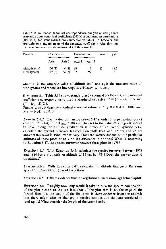
Table 5.14 Detrended canonical correspondence analysis of rising shorevegetation data: canonical coefficients (100 X c) and intra-set correlations(100 X r) for standardized environmental variables. In brackets, theapproximate standard errors of the canonical coefficients. Also given arethe mean and standard deviation (s.d.) of the variables.

Variable

Altitude (cm)Time (years)

Coefficients

Axis 1

100 (3)12(3)

Axis 2

4(4)-34 (3)

Correlations

Axis 1

997

Axis 2

19-99

mean

223

s.d.

18.52.9

where zx is the numeric value of altitude (cm) and z2 is the numeric value oftime (years) and where the intercept is, arbitrary, set to zero.

Hint: note that Table 5.14 shows standardized canonical coefficients, i.e. canonicalcoefficients corresponding to the standardized variables z* = (z, - 22)/18.5 andz2* = (z2-3)/2.9.Similarly, show that the standard errors of estimate of c, = 0.054 is 0.0016 andof c2 = 0.041 is 0.010.

Exercise 5.6.2 Each value of x in Equation 5.47 stands for a particular speciescomposition (Figures 5.8 and 5.18) and changes in the value of x express speciesturnover along the altitude gradient in multiples of s.d. With Equation 5.47,calculate the species turnover between two plots that were 15 cm and 25 cmabove water level in 1984, respectively. Does the answer depend on the particularaltitudes of these plots or only on the difference in altitude? What is, accordingto Equation 5.47, the species turnover between these plots in 1978?

Exercise 5.6.3 With Equation 5.47, calculate the species turnover between 1978and 1984 for a plot with an altitude of 15 cm in 1984? Does the answer dependon altitude?

Exercise 5.6.4 With Equation 5.47, calculate the altitude that gives the samespecies turnover as one year of succession.

Exercise 5.6.5 Is there evidence that the vegetational succession lags behind uplift?

Exercise 5.6.6 Roughly how long would it take to turn the species compositionof the plot closest to the sea into that of the plot that is on the edge of theforest? Hint: use the length of the first axis. Is there evidence from the analysisthat there might also be changes in species composition that are unrelated toland uplift? Hint: consider the length of the second axis.

168

5.11 Solutions to exercises

Exercise 5.1 Correspondence analysis: the algorithm

Exercise 5.1.1 The centroid of the site scores is z — ( 4 X 1 + 2 X 2 + 1X 3 + 3 X 4 + 2 X 5 ) / 1 2 = 2.750 and their dispersion is s2 = [4 X (1 - 2.750)2

+ ... + 2 X (5 - 2.750)2]/12 = 2.353, thus s = 1.5343. The standardized initialscore for the first site is thus x, = (1 - 2.750)/1.5343 = -1.141. The other scoresare listed on the second line of Table 5.15.

Exercise 5.1.2 In the first iteration cycle at Step 2, we obtain for Species C,for example, the score [2 X (-0.489) + 1 X 0.815)]/(2 + 1) = -0.054, and forSite 5 at Step 3, the score (0.815 - 0.228)/(l + 1) = 0.294. The dispersion ofthe species scores in the first iteration cycle is 5 = (2 X 0.1632 + 2 X 0.8152

+ 3 X 0.0542 + 5 X 0.2282)/12 = 0.138. See further Table 5.15. In the iterationsshown z = 0.000, apart from Iteration 3, where z = -0.001 (Step 5). The rearrangeddata table shows a Petrie matrix (Subsection 5.2.3).

Exercise 5.1.3 The standardized site scores obtained in the 19th and 20th iterationare equal within the accuracy of two decimal places; so the iteration process hasconverged (Table 5.15). The eigenvalue of the first axis is X{ = 0.7799, the valueof s calculated last. Equation 5.2 does not hold true for the final site and speciesscores. But the site scores calculated in Step 3 are weighted averages of the speciesscores and are divided in the 20th iteration by s = 0.7799 to obtain the finalsite scores. On convergence, s equals the eigenvalue X; thus the final site andspecies scores satisfy the relation X xt = I£L, yki ukl'Lk

nL]yki. Applying Steps 3,(4) and 5 to the eigenvector (the scores xt) thus transforms the eigenvector intoa multiple of itself. The multiple is the 'eigenvalue' of the eigenvector. Note that5 equals X within arithmetic accuracy.

Exercise 5.1.4 In Step 4.2, we obtain v = [4 X (-1.141) X 0.10 + 2 X (-0.489)X (-0.53) + 1 X 0.163 X 2.00 + 3 X 0.815 X (-0.53) + 2 X 1.466 X 1.11]/12 = 0.2771 and for Site 1 at Step 4.3, the score -1.141 -0.277 1 X 0.10 =-1.169. See further the first four lines of Table 5.16.

Exercise 5.1.5 See Table 5.16.

Exercise 5.1.6 The configuration of the site points looks like the letter V, withSite 1 at the bottom and Sites 2 and 3 at the two extremities. This is the archeffect of CA (Section 5.2.3).

Exercise 5.2 Adding extra sites and species to a CA ordination

Exercise 5.2.1 In CA, Equation 5.1 is used to obtain species scores from sitescores. Thus the score for Hippophae rhamnoides is [1 X 0.09 + 2 X (-0.31)

169

Table 5.15 Two-way weighted averaging algorithm applied to the data of Exercise 5.1 toobtain the first ordination axis of CA. The initial site scores (Line 1) are first standardized(Line 2). The values in brackets are rank numbers of the scores of the line above. Column1, iteration number; Column 2, step number in Table 5.2 ; Column 3, x is site score andu is species score; Column 4, dispersion of the species scores (8) when preceded by w,or otherwise the square root of the dispersion of the site scores of the line above (s).

Column

1

00111222333444555

202020

2

15235235235235235

235

3

X

X

uX

X

uX

X

uX

X

uX

X

uX

X

uX

X

4

1.53430.1375

0.30120.6885

0.69530.7171

0.71930.7342

0.73830.7498

0.75290.7606

0.7800

0.7799

Sites

1

1.000-1.141

-0.212-0.704

-0.393-0.567

-0.322-0.448

-0.251-0.340

-0.185-0.246(3)

0.0810.104(3)

2

2.000-0.489

-0.054-0.179

-0.283-0.408

-0.465-0.646

-0.628-0.851

-0.764-1.015(1)

-1.193-1.530(1)

3

3.0000.163

0.8152.706

1.8412.646

1.8682.597

1.8652.526

1.8402.444(5)

1.5561.995(5)

4

4.0000.815

-0.148-0.491

-0.402-0.580

-0.426-0.592

-0.436-0.591

-0.440-0.584(2)

-0.409-0.524(2)

5

5.0001.466

0.2940.976

0.7581.089

0.8151.133

0.8521.154

0.8751.162(4)

0.8671.112(4)

Species

A

-0.163(2)

-0.598(1)

-0.574(1)

-0.520(2)

-0.466(2)

-0.211(2)

B C D

0.815-0.054-0.228(4)

1.841(4)

(3) (1)

-0.283 -0.325(3) (2)

1.868-0.465-0.238(4) (2) (3)

1.865-0.628-0.161(4) (1) (3)

1.840-0.764-0.091(4)

1.556(4)

(1) (3)

-1.193 0.178(1) (3)

+ 1 X (-0.68)]/(l + 2 + 1) = -0.30, for Poa annua -0.33 and for Ranunculusacris -0.19. All three species come in Table 5.1c between Elymus repens andLeontodon autumnalis. The plots asked for suggest unimodal response curvesfor Hippophae rhamnoides and Poa annua, but a bimodal curve for Ranunculusacris. The species score is the centroid (centre of gravity) of the site scores inwhich they occur. The score gives an indication of the optimum of the responsecurve for the former two species, but has no clear meaning for the latter species.In general, species with a score close to the centre of the ordination may eitherbe unimodal, bimodal or unrelated to the axes (Subsection 5.2.5).

Exercise 5.2.2 The weighted average for the site is [3 X (-0.65) + 5 X (-0.50)+ 4 X (-0.39)]/(3 + 5 + 4) = -0.50, which must be divided as in Exercise 5.1.3by X (= 0.536) to obtain the site score -0.93. If we calculated the score for the

170

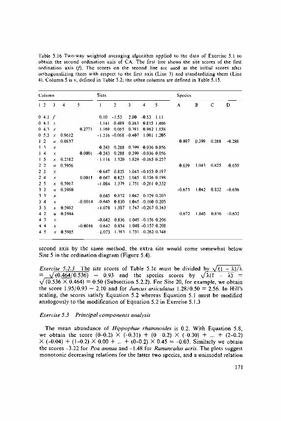
Table 5.16 Two-way weighted averaging algorithm applied to the data of Exercise 5.1 toobtain the second ordination axis of CA. The first line shows the site scores of the firstordination axis (/). The scores on the second line are used as the initial scores afterorthogonalizing them with respect to the first axis (Line 3) and standardizing them (Line4). Column 5 is v, defined in Table 5.2; the other columns are defined in Table 5.15.

Column Sites Species

1

00001111222233334444

2

4.14.14.35.32345234523452345

3

/X

X

X

uX

X

X

uX

X

X

uX

X

X

uX

X

X

4

0.96120.0837

0.21820.5956

0.59670.5980

0.59820.5984

0.5985

5

0.2771

0.0001

-0.0011

-0.0014

-0.0016

1

0.10-1.141-1.169-1.216

-0.243-0.243-1.114

-0.647-0.647-1.084

-0.645-0.645-1.078

-0.642-0.642-1.073

2

-1.53-0.489-0.065-0.068

0.2880.2881.320

0.8250.8231.379

0.8320.8301.387

0.8360.8341.393

3

2.000.163

-0.391-0.407

0.3990.3991.829

1.0431.0451.751

1.0421.0451.747

1.0451.0481.751

4

-0.530.8150.9621.001

5

1.111.4661.1581.205

-0.036 0.056-0.036 0.056-0.165

-0.155-0.156-0.261

-0.159-0.160-0.267

0.257

0.1970.1980.332

0.2030.2050.343

-0.156 0.206-0.157-0.262

0.2080.348

-0.107 0.399 0.288 -0.288

-0.639 1.043 0.825 -0.650

-0.673 1.042 0.832 -0.636

-0.672 1.045 0.836 -0.632

second axis by the same method, the extra site would come somewhat belowSite 5 in the ordination diagram (Figure 5.4).

Exercise 5.2.3 The site scores of Table 5.1c must be divided by \ (= v70.464/0.536) = 0.93 and the species scores by \A(1 - )V (0.536 X 0.464) = 0.50 (Subsection 5.2.2). For Site 20, for example, we obtainthe score 1.95/0.93 = 2.10 and for Juncus articulatus 1.28/0.50 = 2.56. In Hill'sscaling, the scores satisfy Equation 5.2 whereas Equation 5.1 must be modifiedanalogously to the modification of Equation 5.2 in Exercise 5.1.3

Exercise 5.3 Principal components analysis

The mean abundance of Hippophae rhamnoides is 0.2. With Equation 5.8,we obtain the score (0-0.2) X (-0.31) + (0 -0.2) X (-0.30) + ... + (2-0.2)X (-0.04) + (1-0.2) X 0.00 4- ... 4- (0-0.2) X 0.45 = -0.03. Similarly we obtainthe scores -3.22 for Poa annua and -1.48 for Ranunculus acris. The plots suggestmonotonic decreasing relations for the latter two species, and a unimodal relation

171

(if any) for the first species. If straight lines are fitted in these plots, the slopeof regression turns out to equal the species score (Subsection 5.3.1). The speciescome at different places in Table 5.5c. For example, Poa annua comes just afterBromus hordaceus. The score for the extra site is calculated by dividing the weightedsum (Equation 5.9) by the eigenvalue: 3.90/471 = 0.008.

Exercise 5.4 Length of gradient in DC A

In DCA, axes are scaled such that the standard deviation (tolerance) of theresponse curve of each species is close to one and is on average equal to one.Each response curve will therefore rise and decline over an interval of about4 s.d. (Figure 3.6; Figure 5.3b). If the length of the first axis equals 1.5 s.d.,the length of the axis covers only a small part of the response curve of eachspecies. Most plots will therefore suggest monotonic curves, although the trueresponse curves may be unimodal (Figure 3.3). If the length of the first axis is10 s.d., the response curves of many species are'contained within the length ofthe axis, so that many of the plots will suggest unimodal response curves.

5.5 Interpretation of joint plot and biplot

Exercise 5.5.1 Inferred rank orders of abundance are for Juncus bufonius

from Figure 5.7 (DCA) sites 12 > 8 > 13 > 9 > 4 « 18from Figure 5.15 (PCA) sites 13%3>4>9%12from Table 5.1a (data) sites 9 = 1 2 > 1 3 > 7 - -

and for Eleocharis palustris

from Figure 5.7 (DCA) sites 16> 14%15>20>8from Figure 5.15 (PCA) sites 16>20>15> 14>19from Table 5.1a (data) Sites 16 > 15 > 8 = 14 = 20.

Exercise 5.5.2 The difference in interpretation is greatest for species that lie atthe centre of the ordination diagram. In a DCA diagram, the inferred abundancedrops with distance from the species point in any direction, whereas in a PCAdiagram the inferred abundance decreases or increases with distance from thespecies point, depending on the direction. This difference is rather unimportantfor species that lie on the edge of the diagram, because the site points all lieon one side of the species point. One comes to the same conclusion by notingthat a species point in a DCA diagram is its inferred optimum; if the optimumlies far outside the region of the sites the inferred abundance changes monotonicallyacross the region of site points (Eleocharis palustris in Figure 5.7).

Exercise 5.6 Detrended canonical correspondence analysis

Exercise 5.6.1 From Table 5.14, we see that the best linear combination is

172

x — 1.00 z* + 0.12 z2*. In terms of unstandardized variables, we obtain x =1.00 X (z, - 22)/18.5 + 0.12 X (z2 - 3)/2.9 = (1.00/18.5)z, + (0.12/2.9)z2 - 22/18.5 - 0.12 X 3/2.9 = 0.054 z, + 0.041 z2 - 1.31. The standard error of cx is0.03/18.5 = 0.00162 and of c2 is 0.03/2.9 = 0.010.

Exercise 5.6.2 The value of x for the plot that was 15 cm above water levelin 1984 is x = 0.054 X 15 + 0.041 X 6 = 1.056 s.d. For the plot 25 cm abovewater level, we obtain x = 0.054 X 25 + 0.041 X 6 = 1.596 s.d. Hence, thespecies turnover is 1.596 - 1.056 = 0.54 s.d. According to Equation 5.47, turnoverdepends only on the difference in altitude between the plots: 0.054 X (25 - 15)= 0.54, and does not depend on the particular altitudes of the plots nor on theyear of sampling. The species turnover between plots differing 10 cm in altitudeis therefore 0.54 s.d. on both occasions of sampling.

Exercise 5.6.3 The value of x for a plot with an altitude of 15 cm in 1984 was1.056 s.d. in 1984 (Exercise 5.6.2) and was 0.054 X 15 + 0.041 X 0 = 0.81 s.d.in 1978. (Note that in the model altitude was not corrected for uplift; hencez, = 15 in 1984 and in 1978.) The species turnover is 1.056 - 0.81 = 0.246 s.d.,which equals 0.041 X 6 s.d. and which is independent of altitude. Hence, eachplot changes about a quarter standard deviation in 6 years.

Exercise 5.6.4 The species turnover rate is 0.041 s.d. per year, whereas the speciesturnover due to altitude is 0.054 s.d. per centimetre. The change in altitude thatresults in 0.041 s.d. species turnover is therefore 0.041/0.054 = 0.76 cm. Anapproximate 95% confidence interval can be obtained for this ratio from thestandard error of cl and c2 and their covariance by using Fieller's theorem (Finney1964). Here the covariance is about zero. In this way, we so obtained the interval(0.4 cm, 1.1 cm).

Exercise 5.6.5 From Exercise 5.6.4, we would expect each particular speciescomposition to occur next year 0.76 cm lower than its present position. Uplift(about 0.5 cm per year) is less; hence, there is no evidence that the vegetationalsuccession lags behind the land uplift. The known uplift falls within the confidenceinterval given above. Further, because the value 0 cm lies outside the confidenceinterval, the effect of uplift on species composition is demonstrated. Upliftapparently drives the vegetational succession without lag.

Exercise 5.6.6 The length of the first axis is 4.4 s.d. From Exercise 5.6.3, weknow that each plot changes about 0.25 s.d. in 6 years. The change from vegetationnear the sea to vegetation at the edge of the forest therefore takes roughly (4.4/0.25) X 6 years *** 100 years. The second axis is 0.9 s.d. and mainly representsthe differences in species composition between the two sampling occasions thatare unrelated to altitude and land uplift. More precisely, the canonical coefficientof time on the second axis is -0.34/2.9 = -0.117. It therefore accounts for 0.117X 6 s.d. = 0.70 s.d. of the length of the second axis, whereas time accountedfor 0.25 s.d. of the length of the first axis. There are apparently more changesgoing on than can be accounted for by uplift.

173

6 Cluster analysis

O.F.R. van Tongeren

6.1 Introduction

6.1.1 Aims and use

For ecological data, cluster analysis is a type of analysis that classifies sites,species or variables. Classification is intrinsic in observation: people observe objectsor phenomena, compare them with other, earlier, observations and then assignthem a name. Therefore one of the major methods used since the start of thestudy of ecology is the rearrangement of data tables of species by sites, followedby the definition of community types, each characterized by its characteristic speciescombination (Westhoff & vander Maarel 1978; Becking 1957). Scientists of differentschools have different ideas about the characterization of community types andthe borders between these types. In vegetation science, for instance, the Scan-dinavian school and the Zurich-Montpellier school differ markedly, the Scan-dinavians emphasizing the dominants and the Zurich-Montpellier school givingmore weight to characteristic and differential species, which are supposed to havea narrower ecological amplitude and are therefore better indicators for theenvironment. Cluster analysis is an explicit way of identifying groups in raw dataand helps us to find structure in the data. However even if there is a continuousstructure in the data, cluster analysis may impose a group structure: a continuumis then arbitrarily partitioned into a discontinuous system of types or classes.

Aims of classification are:- to give information on the concurrence of species (internal data structure)- to establish community types for descriptive studies (syntaxonomy and map-

ping)- to detect relations between communities and the environment by analysis of

the groups formed by the cluster analysis with respect to the environmentalvariables (external analysis).

In Chapter 6, an introduction will be given to several types of cluster analysis.This chapter aims at a better understanding of the properties of several methodsto facilitate the choice of a method, without pretending to show you how tofind the one and only best structure in your data. It is impossible to choosea 'best' method because of the heuristic nature of the methods. If there is a markedlydiscontinuous structure, it will be detected by almost any method, a continuousstructure will almost always be obscured by cluster analysis.

174

6.1.2 Types of cluster analysis

There are several types of cluster analysis, based on different ideas about thecluster concept. Reviews are found mainly in the taxonomic literature (Lance& Williams 1967; Dunn & Everitt 1982). Here a brief summary will be givenof the main groups.

A major distinction can be made between divisive and agglomerative methods.Divisive methods start with all objects (in ecology mostly samples; in taxonomyoperational taxonomic units, OTUs) as a group. First this group is divided intotwo smaller groups, which is repeated subsequently for all previously formed groups,until some kind of 'stopping rule' is satisfied. The idea of this way of clusteringis that large differences should prevail over the less important smaller differences:the global structure of a group should determine the subgroups. Alternativelyagglomerative methods start with individual objects, which are combined intogroups by collection of objects or groups into larger groups. Here 'local' similarityprevails over the larger differences. Divisive methods will be described in Section6.3, and agglomerative methods in Section 6.2. Most agglomerative methods requirea similarity or dissimilarity matrix (site by site) to start from. Several indicesof (dis)similarity will be introduced in Subsection 6.2.3.

A second way of distinguishing methods is to classify them by hierarchicaland non-hierarchical methods. Hierarchical methods start from the idea that thegroups can be arranged in a hierarchical system. In ecology, one could say thata certain difference is more important than another one and therefore shouldprevail: be expressed at a higher hierarchical level. Non-hierarchical methods donot impose such a hierarchical structure on the data. For data reduction, non-hierarchical methods are usually used.

Non-hierarchical classification handles- redundancy: sites that are much like many other sites are grouped without

considering the relations to other less similar sites- noise: before subsequent hierarchical clustering, a 'composite sample' may be

constructed- outliers, which can be identified because they appear in small clusters or as

single samples.

6.2 Agglomerative methods

6.2.1 Introduction

Agglomerative cluster analysis starts from single objects, which are agglomeratedinto larger clusters. In many sciences, agglomerative techniques are employed muchmore frequently than divisive techniques. The historical reason for this is theinefficient way early polythetic divisive techniques used computer resources, whilethe agglomerative ones were more efficient. Now, the opposite seems true.Nevertheless, there is a very large range of agglomerative techniques, eachemphasizing other aspects of the data and therefore very useful.

All agglomerative methods share the idea that some kind of (dis)similarity

175

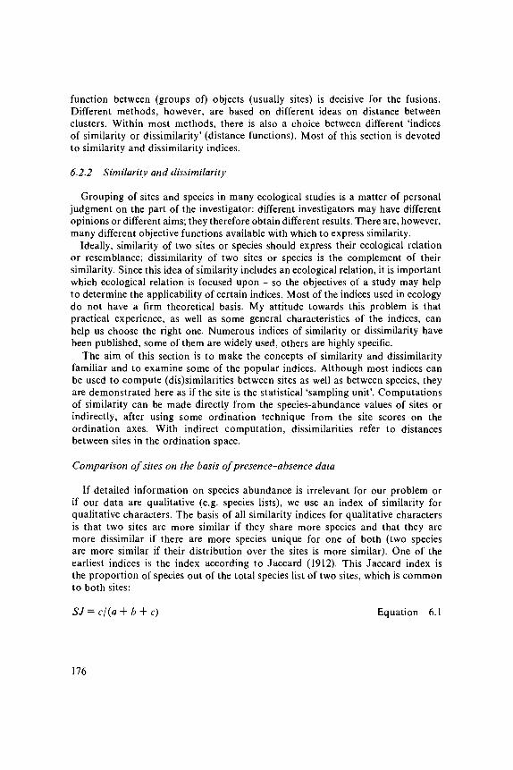
function between (groups of) objects (usually sites) is decisive for the fusions.Different methods, however, are based on different ideas on distance betweenclusters. Within most methods, there is also a choice between different 'indicesof similarity or dissimilarity' (distance functions). Most of this section is devotedto similarity and dissimilarity indices.

6.2.2 Similarity and dissimilarity

Grouping of sites and species in many ecological studies is a matter of personaljudgment on the part of the investigator: different investigators may have differentopinions or different aims; they therefore obtain different results. There are, however,many different objective functions available with which to express similarity.

Ideally, similarity of two sites or species should express their ecological relationor resemblance; dissimilarity of two sites or species is the complement of theirsimilarity. Since this idea of similarity includes an ecological relation, it is importantwhich ecological relation is focused upon - so the objectives of a study may helpto determine the applicability of certain indices. Most of the indices used in ecologydo not have a firm theoretical basis. My attitude towards this problem is thatpractical experience, as well as some general characteristics of the indices, canhelp us choose the right one. Numerous indices of similarity or dissimilarity havebeen published, some of them are widely used, others are highly specific.

The aim of this section is to make the concepts of similarity and dissimilarityfamiliar and to examine some of the popular indices. Although most indices canbe used to compute (dis)similarities between sites as well as between species, theyare demonstrated here as if the site is the statistical 'sampling unit'. Computationsof similarity can be made directly from the species-abundance values of sites orindirectly, after using some ordination technique from the site scores on theordination axes. With indirect computation, dissimilarities refer to distancesbetween sites in the ordination space.

Comparison of sites on the basis of presence-absence data

If detailed information on species abundance is irrelevant for our problem orif our data are qualitative (e.g. species lists), we use an index of similarity forqualitative characters. The basis of all similarity indices for qualitative charactersis that two sites are more similar if they share more species and that they aremore dissimilar if there are more species unique for one of both (two speciesare more similar if their distribution over the sites is more similar). One of theearliest indices is the index according to Jaccard (1912). This Jaccard index isthe proportion of species out of the total species list of two sites, which is commonto both sites:

SJ — c/(a + b + c) Equation 6.1

176

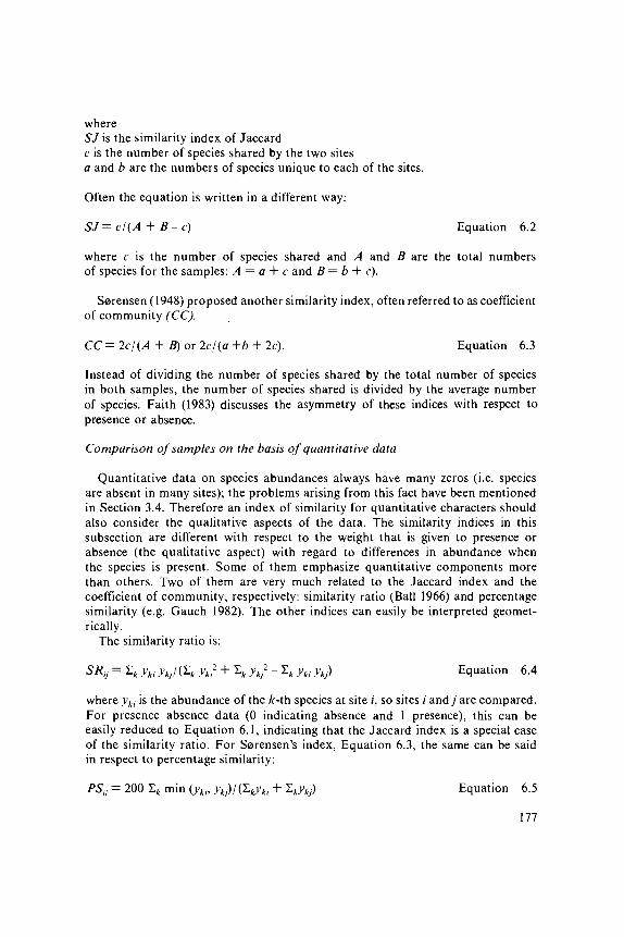
whereSJ is the similarity index of Jaccardc is the number of species shared by the two sitesa and b are the numbers of species unique to each of the sites.

Often the equation is written in a different way:

SJ = c\ (A + B - c) Equation 6.2

where c is the number of species shared and A and B are the total numbersof species for the samples: A — a + c and B — b + c).

Sorensen (1948) proposed another similarity index, often referred to as coefficientof community (CC).

CC = 2c/ (A + B) or 2cI (a +b + 2c). Equation 6.3

Instead of dividing the number of species shared by the total number of speciesin both samples, the number of species shared is divided by the average numberof species. Faith (1983) discusses the asymmetry of these indices with respect topresence or absence.

Comparison of samples on the basis of quantitative data

Quantitative data on species abundances always have many zeros (i.e. speciesare absent in many sites); the problems arising from this fact have been mentionedin Section 3.4. Therefore an index of similarity for quantitative characters shouldalso consider the qualitative aspects of the data. The similarity indices in thissubsection are different with respect to the weight that is given to presence orabsence (the qualitative aspect) with regard to differences in abundance whenthe species is present. Some of them emphasize quantitative components morethan others. Two of them are very much related to the Jaccard index and thecoefficient of community, respectively: similarity ratio (Ball 1966) and percentagesimilarity (e.g. Gauch 1982). The other indices can easily be interpreted geomet-rically.

The similarity ratio is:

SRfj = I* yki ykJl (2* ykl2 + I , yk? - lk yki ykj) Equation 6.4

where yki is the abundance of the k-\h species at site /, so sites / andy are compared.For presence-absence data (0 indicating absence and 1 presence), this can beeasily reduced to Equation 6.1, indicating that the Jaccard index is a special caseof the similarity ratio. For Sorensen's index, Equation 6.3, the same can be saidin respect to percentage similarity:

PSy = 200 2* min (ykh yk/)l(Zkyki + !,>>,,) Equation 6.5

177

Figure 6.1 Five sites (1-5) in a three-dimensional space of which the axes are the threspecies A, B and C. Site 1 is characterized by low abundance of species A and specieC, and absence of species B. In site 2, species A is dominant, species B is less importanand species C is absent. Sites 3 and 4 are monocultures of species B and C, respectivel)Site 5 has a mixture of all three species.

where min (ykh ykj) is the minimum of yki and ykj.

Some indices can be explained geometrically. To explain these indices, it inecessary to represent the sites by a set of points in a multi-dimensional spac(with as many dimensions as there are species). One can imagine such a spacwith a maximum of three species (Figure 6.1) but conceptually there is no differencif we use more species (see Subsection 5.3.3).

The position of a site is given by using the abundances of the species as coordinate(Figure 6.1), and therefore sites with similar species composition occupy nearbpositions in species space. The Euclidean Distance, ED, between two sites is aobvious measure of dissimilarity:

ED — \J I,k (ykj - yk/)2 Equation 6.

Figure 6.1 shows that quantitative aspects play a major role in Euclidean Distancethe distance between Sites 1 and 2, which share one species, is much larger thathe distance between Sites 1 and 3, not sharing a species.

More emphasis is given to qualitative aspects by not considering a site aspoint but as a vector (Figure 6.2). Understandably, the direction of this vectotells us something about the relative abundances of species. The similarity otwo sites can be expressed as some function of the angle between the vectorof these sites. Quite common is the use of the cosine (or Ochiai coefficient):

= lk yki ykj Equation 6.

A dissimilarity index that is more sensitive to qualitative aspects than the EuclideaDistance is the chord distance:

178

Figure 6.2 The same space as in Figure 6.1. Samples are now indicated by vectors. Crossesindicate where the sample vectors intersect the unit sphere (broken lines). Note that thedistance between 1' and 2 ' is much lower than the distance between either of them and3'. The angle between sample vectors 1 and 3 is indicated by a.

[ykiIVk y*p - ykjICLk ykjff Equation 6.8

This chord distance is geometrically represented by the distance between the pointswhere the sample vectors intersect the unit sphere (Figure 6.2).

Conversion of similarity to dissimilarity and vice versa

For some applications, one may have to convert a similarity index into adissimilarity index. This conversion must be made if, for instance, no dissimilarityindex with the desired properties is available, but the cluster algorithm needsan index of dissimilarity. For cluster algorithms merely using the rank order ofdissimilarities, any conversion reversing the rank order is reasonable, but caremust be taken for cluster algorithms that use the dissimilarities in a quantitativeway (as forming an interval or ratio scale (Subsection 2.4.2). We mention twoways of making the conversion:

- subtracting each similarity value from a certain value: in this way the intervalsbetween the values are preserved. Bray & Curtiss (1957), for instance, subtractsimilarity values from the expected similarity among replicate samples, theso-called internal association. In practice, the best estimate of internal as-sociation (IA) is the maximum similarity observed. Thus percentage similarityis converted to percentage distance, PD, using this subtraction:

PD^ IA- PS Equation 6.9

179

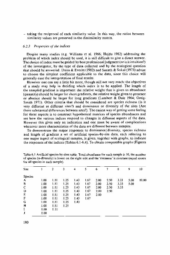
- taking the reciprocal of each similarity value. In this way, the ratios betweensimilarity values are preserved in the dissimilarity matrix.

6.2.3 Properties of the indices

Despite many studies (e.g. Williams et al. 1966; Hajdu 1982) addressing theproblem of which index should be used, it is still difficult to give a direct answer.The choice of index must be guided by best professional judgment (or is it intuition?)of the investigator, by the type of data collected and by the ecological questionthat should be answered. Dunn & Everitt (1982) and Sneath & Sokal (1973) adviseto choose the simplest coefficient applicable to the data, since this choice willgenerally ease the interpretation of final results.

However one can say a little bit more, though still not very much: the objectivesof a study may help in deciding which index is to be applied. The length ofthe sampled gradient is important: the relative weight that is given to abundance(quantity) should be larger for short gradients, the relative weight given to presenceor absence should be larger for long gradients (Lambert & Dale 1964; Greig-Smith 1971). Other criteria that should be considered are species richness (Is itvery different at different sites?) and dominance or diversity of the sites (Arethere substantial differences between sites?). The easiest way of getting some feelingfor these aspects is to construct hypothetical matrices of species abundances andsee how the various indices respond to changes in different aspects of the data.However this gives only an indication and one must be aware of complicationswhenever more characteristics of the data are different between samples.

To demonstrate the major responses to dominance/diversity, species richnessand length of gradient a set of artificial species-by-site data, each referring toone major aspect of ecological samples, is given, together with graphs, to indicatethe responses of the indices (Tables 6.1-6.4). To obtain comparable graphs (Figures

Table 6.1 Artificial species-by-sites table. Total abundance for each sample is 10, the numberof species (a-diversity) is lower on the right side and the 'evenness' is constant (equal scoresfor all species in each sample).

Site

SpeciesABCDEFGHIJ

i :

1.001.00 11.001.001.001.001.001.001.001.00

>

.11

.11

.11

.11

.11

.111.11.11

1.11

3 '

1.251.251.251.251.251.251.251.25

[

.43

.43

.43

.431.431.431.43

5

1.671.671.671.671.671.67

6

2.002.002.002.002.00

7

2.502.502.502.50

8

3.333.333.33

9

5.005.00

10

10.00

180

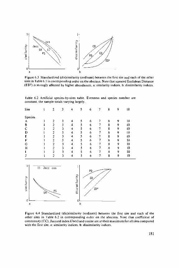
Figure 6.3 Standardized (dis)similarity (ordinate) between the first site and each of the othersites in Table 6.1 in corresponding order on the abscissa. Note that squared Euclidean Distance(ED2) is strongly affected by higher abundances, a: similarity indices, b: dissimilarity indices.

Table 6.2 Artificial species-by-sites table. Evenness and species number areconstant, the sample totals varying largely.

Site 10

SpeciesABCDEFGHIJ

9999999999

10101010101010101010

CC Jacc cos

Figure 6.4 Standardized (dis)similarity (ordinate) between the first site and each of theother sites in Table 6.2 in corresponding order on the abscissa. Note that coefficient ofcommunity (CC), Jaccard index (Jacc) and cosine are at their maximum for all sites comparedwith the first site, a: similarity indices, b: dissimilarity indices.

181

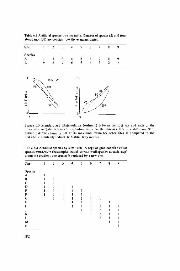
Table 6.3 Artificial species-by-sites table. Number of species (2) and totalabundance (10) are constant but the evenness varies.

Site 1

SpeciesA 1B 9

X ^ \ Jacc

S R \

cc

Figure 6.5 Standardized (dis)similarity (ordinate) between the first site and each of theother sites in Table 6.3 in corresponding order on the abscissa. Note the difference withFigure 6.4: the cosine is not at its maximum value for other sites as compared to thefirst site, a: similarity indices, b: dissimilarity indices.

Table 6.4 Artificial species-by-sites table. A regular gradient with equalspecies numbers in the samples, equal scores for all species: at each 'step'along the gradient one species is replaced by a new one.

Site

SpeciesABCDEFGHIJKLMN

1 2 5

1111

11111

11 11 11 11 11 1

11111

1111

111

182

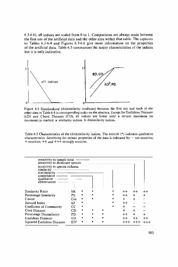
6.3-6.6), all indices are scaled from 0 to 1. Comparisons are always made betweenthe first site of the artificial data and the other sites within that table. The captionsto Tables 6.1-6.4 and Figures 6.3-6.6 give more information on the propertiesof the artificial data. Table 6.5 summarizes the major characteristics of the indicesbut it is only indicative.

1- 1-

all indicesED2, PD

Figure 6.6 Standardized (dis)similarity (ordinate) between the first site and each of theother sites in Table 6.4 in corresponding order on the abscissa. Except for Euclidean Distance(ED) and Chord Distance (CD), all indices are linear until a certain maximum (orminimum) is reached, a: similarity indices, b: dissimilarity indices.

Table 6.5 Characteristics of the (dis)similarity indices. The asterisk (*) indicates qualitativecharacteristics. Sensitivity for certain properties of the data is indicated by: — not sensitive;-f sensitive; + + and + + + strongly sensitive.

sensitivity to sample totalsensitivity to dominant species _sensitivity to species richness —similaritydissimilarityquantitativequalitativeauuitviauuu

Similarity RatioPercentage SimilarityCosineJaccard IndexCoefficient of CommunityCord DistancePercentage DissimilarityEuclidean DistanceSquared Euclidean Distance

nSRPSCosSJCCCDPDEDED2

183

6.2.4 Transformation, standardization and weighting

Transformation, standardization and weighting of data are other ways of lettingcertain characteristics of the data express themselves more or less strongly. Thisparagraph is meant to give you some idea of how certain manipulations can bemade with the data and what are the reasons for and the consequences oftransformations and standardizations.

Transformation

Transformations are possible in many different ways. Most transformations usedin ecology are essentially non-linear transformations: the result of such trans-formations is that certain parts of the scale of measurement for the variablesare shrunk, while other parts are stretched.

Logarithmic transformation.yfj = l°ge ytj or (if zeros are present) yj=loge (ytj + 1) Equation 6.10

This transformation is often used for three essentially different purposes:- to obtain the statistically attractive property of normal distribution for log-

normally distributed variables (as in Subsection 2.4.4)- to give less weight to dominant species, in other words to give more weight

to qualitative aspects of the data- in environmental variables, to reflect the linear response of many species to

the logarithm of toxic agents or (in a limited range) to the logarithm of nutrientconcentrations. Instead o f '+1 ' , take the minimum non-zero value.

Square-root transformation.y* = y^2 Equation 6.11

This transformation is used- before analysis of Poisson-distributed variables (e.g. number of individuals

of certain species caught in a trap over time)- to give less weight to dominant species.

Exponential transformation.yif = ayiJ. Equation 6.12

If a is a real number greater than 1, the dominants are emphasized.

Transformation to an ordinal scale. The species abundances are combined intoclasses. The higher the class number, the higher the abundance. A higher classnumber always means a higher abundance, but an equal class number does notalways mean an equal abundance: intervals between classes are almost meaningless.Dependent on the class limits, one can influence the results of a classificationin all possible ways. An extreme is the transformation to presence-absence scale

184

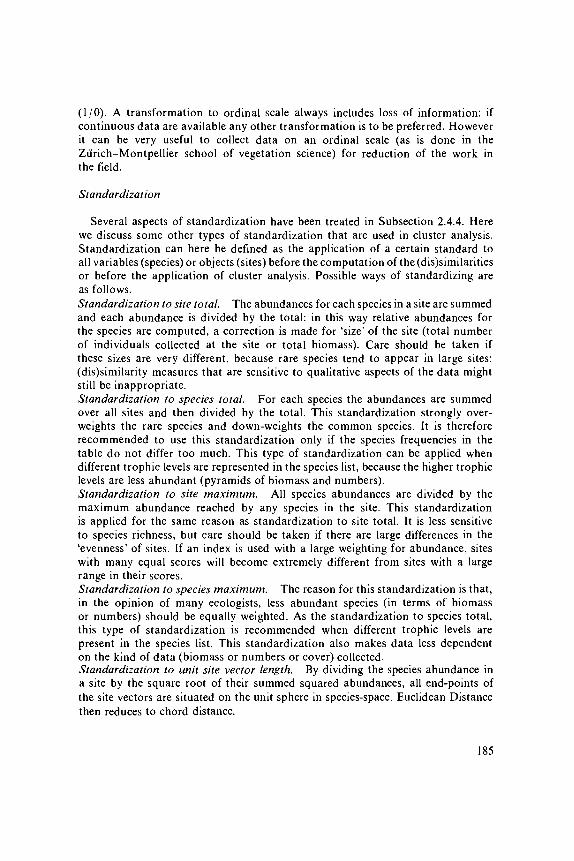
(1/0). A transformation to ordinal scale always includes loss of information: ifcontinuous data are available any other transformation is to be preferred. Howeverit can be very useful to collect data on an ordinal scale (as is done in theZurich-Montpellier school of vegetation science) for reduction of the work inthe field.

Standardization

Several aspects of standardization have been treated in Subsection 2.4.4. Herewe discuss some other types of standardization that are used in cluster analysis.Standardization can here be defined as the application of a certain standard toall variables (species) or objects (sites) before the computation of the (dis)similaritiesor before the application of cluster analysis. Possible ways of standardizing areas follows.Standardization to site total. The abundances for each species in a site are summedand each abundance is divided by the total: in this way relative abundances forthe species are computed, a correction is made for 'size' of the site (total numberof individuals collected at the site or total biomass). Care should be taken ifthese sizes are very different, because rare species tend to appear in large sites:(dis)similarity measures that are sensitive to qualitative aspects of the data mightstill be inappropriate.Standardization to species total. For each species the abundances are summedover all sites and then divided by the total. This standardization strongly over-weights the rare species and down-weights the common species. It is thereforerecommended to use this standardization only if the species frequencies in thetable do not differ too much. This type of standardization can be applied whendifferent trophic levels are represented in the species list, because the higher trophiclevels are less abundant (pyramids of biomass and numbers).Standardization to site maximum. All species abundances are divided by themaximum abundance reached by any species in the site. This standardizationis applied for the same reason as standardization to site total. It is less sensitiveto species richness, but care should be taken if there are large differences in the'evenness' of sites. If an index is used with a large weighting for abundance, siteswith many equal scores will become extremely different from sites with a largerange in their scores.Standardization to species maximum. The reason for this standardization is that,in the opinion of many ecologists, less abundant species (in terms of biomassor numbers) should be equally weighted. As the standardization to species total,this type of standardization is recommended when different trophic levels arepresent in the species list. This standardization also makes data less dependenton the kind of data (biomass or numbers or cover) collected.Standardization to unit site vector length. By dividing the species abundance ina site by the square root of their summed squared abundances, all end-points ofthe site vectors are situated on the unit sphere in species-space. Euclidean Distancethen reduces to chord distance.

185

Weighting

There are several reasons for weighting species or sites. Depending on the reasonfor down-weighting several kinds of down-weighting can be applied.Down-weighting of rare species. A lower weight dependent on the speciesfrequency, is assigned to rare species to let them influence the final result to alesser extent. This should be done if the occurrence of these species is merelyby chance and if the (dis)similarity index or cluster technique is sensitive to rarespecies.Down-weighting of species indicated by the ecologist. A lower weight is assignedto species (or sites) that are less reliable (determination of a species is difficult;a sample is taken by an inexperienced field-worker) or to species that are ecologicallyless relevant (planted trees; the crop species in a field). This kind of down-weightingis ad hoc and therefore arbitrary.

6.2.5 Agglomerative cluster algorithms

All agglomerative methods are based on fusion of single entities (sites) or clusters(groups of sites) into larger groups. The two groups that closest resemble eachother are always fused, but the definition of (dis)similarity between groups differsbetween methods.

Often the results of hierarchical clustering are presented in the form of adendrogram (tree-diagram, e.g. Figure 6.8). Such a dendrogram shows the relationsbetween sites and groups of sites. The hierarchical structure is indicated by thebranching pattern.

Single-linkage or nearest-neighbour clustering

The distance between two clusters is given by the minimum distance that canbe measured between any two members of the clusters (Figure 6.7). A dendrogramof the classification of the Dune Meadow Data with single-linkage clustering,

Figure 6.7 Distances (solid lines) between clusters in single linkage: samples within thesame cluster are indicated with the same symbol.

186

0.21

0.4

0.6

0.£

1.07 10 5 2 3 4 8 9 11 18 12 13 15 20 16 1 14 17 19

Figure 6.8 Dendrogram of single linkage, using the Dune Meadow Data and the similarityratio.

Figure 6.9 Hypothetical example of 'chaining', a problem occurring in single-linkageclustering.

using similarity ratio, is given in Figure 6.8. The dendrogram shows us that thereare not very well defined clusters: our data are more or less continuous. Single-linkage clustering can be used very well to detect discontinuities in our data.For other research in community ecology, it is not appropriate because of itstendency to produce straggly clusters, distant sites being connected by chains ofsites between them (Figure 6.9).

187

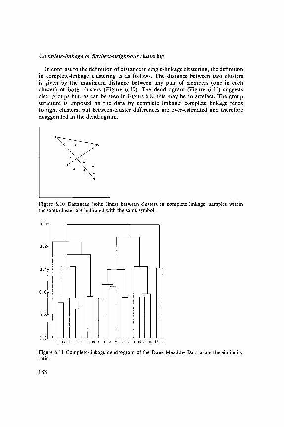
Complete-linkage or furthest-neighbour clustering

In contrast to the definition of distance in single-linkage clustering, the definitionin complete-linkage clustering is as follows. The distance between two clustersis given by the maximum distance between any pair of members (one in eachcluster) of both clusters (Figure 6.10). The dendrogram (Figure 6.11) suggestsclear groups but, as can be seen in Figure 6.8, this may be an artefact. The groupstructure is imposed on the data by complete linkage: complete linkage tendsto tight clusters, but between-cluster differences are over-estimated and thereforeexaggerated in the dendrogram.

Figure 6.10 Distances (solid lines) between clusters in complete linkage: samples withinthe same cluster are indicated with the same symbol.

0.0

0.2

0.4

0.6

0.8

1.0

Q n1 2 10 5 6 7 11 18 3 4 8 9 12 13 14 15 20 16 17 19

Figure 6.11 Complete-linkage dendrogram of the Dune Meadow Data using the similarityratio.

188

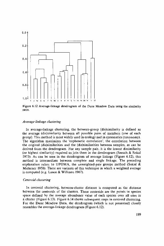
0.0

0.2

0.4

0.6

0.8

1.0

I

7 11 18 3 4 9 12 13 14 15 20 16 17 19

Figure 6.12 Average-linkage dendrogram of the Dune Meadow Data using the similarityratio.

Average-linkage clustering

In average-linkage clustering, the between-group (dis)similarity is defined asthe average (dis)similarity between all possible pairs of members (one of eachgroup). This method is most widely used in ecology and in systematics (taxonomy).The algorithm maximizes the 'cophenetic correlation', the correlation betweenthe original (dis)similarities and the (dis)similarities between samples, as can bederived from the dendrogram. For any sample pair, it is the lowest dissimilarity(or highest similarity) required to join them in the dendrogram (Sneath & Sokal1973). As can be seen in the dendrogram of average linkage (Figure 6.12), thismethod is intermediate between complete and single linkage. The precedingexplanation refers to UPGMA, the unweighted-pair groups method (Sokal &Michener 1958). There are variants of this technique in which a weighted averageis computed (e.g. Lance & Williams 1967).

Centroid clustering

In centroid clustering, between-cluster distance is computed as the distancebetween the centroids of the clusters. These centroids are the points in speciesspace defined by the average abundance value of each species over all sites ina cluster (Figure 6.13). Figure 6.14 shows subsequent steps in centroid clustering.For the Dune Meadow Data, the dendrogram (which is not presented) closelyresembles the average-linkage dendrogram (Figure 6.12).

189

Figure 6.13 Between-cluster distances (solid lines) in centroid clustering: samples withinthe same cluster are indicated with the same symbol; cluster centroids are indicated bysquares.

O A <>•<>

<>•<> o o•

o

Figure 6.14 Subsequent steps in centroid clustering. Sites belonging to the same clusterare indicated with the same open symbol. Cluster centroids are indicated by the correspondingfilled symbols. Upon fusion of two clusters, the symbols of sites change to indicate thenew cluster to which they belong.

190

Ward's method or minimum variance clustering

Ward's method, also known as Orloci's (1967) error sum of squares clustering,is in some respects similar to average-linkage clustering and centroid clustering.Between-cluster distance can either be computed as a squared Euclidean distancebetween all pairs of sites in a cluster weighted by cluster size (resembling average-linkage clustering) or as an increment in squared distances towards the clustercentroid when two clusters are fused (resembling centroid clustering). Penalty bysquared distance and cluster size makes the clusters tighter than those in centroidclustering and average linkage, and more like those obtained in complete linkage.The algorithm proceeds as follows: with all samples in a separate cluster, the sumof squared distances is zero, since each sample coincides with the centroid of itscluster. In each step, the pair of clusters is fused, which minimizes the total within-group sum of squares (Subsection 3.2.1, residual sum of squares), which is equalto minimizing the increment (d£) in the total sum of squares:

&E=Ep+q-Ep-Eq

whereE is the total error sum of squaresEp+q is the within-group sums of squares for the cluster in which p and q arefused togetherEp and Eq the sums of squares for the individual clusters p and q.

The within-group sum of squares for a cluster is:

where the first summation is over all members of cluster/? and the second summationis over all species.

The dendrograms of Ward's clustering, average linkage and complete linkageusing squared Euclidean Distance are given in Figure 6.15.

6.3 Divisive methods

6.3.1 Introduction

Divisive methods have long been neglected. The reason for this is that theywere developed in the early years of numerical data analysis. At that time theyfailed either because of inefficiency (too many computational requirements) orbecause the classification obtained was inappropriate. Williams & Lambert (1960)developed the first efficient method for divisive clustering: association analysis.This method is monothetic: divisions are made on the basis of one attribute (e.g.character or species). Although it is not used very often now, some authors stilluse association analysis or variations of association analysis (e.g. Kirkpatrick et

191

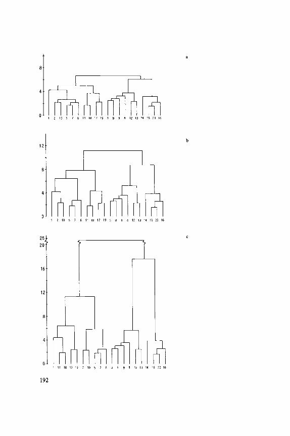
1 2 10 5 7 6 11 18 17 19 3 8 9 4 12 13 14 15 20 16

12-

\\fuh2 10 5 7 6 11 18 17 19 3 8 9 4 12 13 14 15 20 16

25120"

16

12

11 18 17 19 2 10 5 7 6 3 8 9 4 12 13 14 15 20 16

192

al. 1985). Subsection 6.3.2 briefly describes association analysis. Efficient polytheticmethods for divisive clustering appeared after Roux & Roux (1967) introducedthe partitioning of ordination space for purposes of classification. Lambert etal. (Williams 1976b) wrote a program to perform a division based on partitioningof the first axis of principal component analysis. A divisive clustering is obtainedby repeating this method of partitioning on the groups obtained in the previousstep. More recently, Hill (Hill et al. 1975; Hill 1979b) developed a method basedon the partitioning of the first axis of CA. Since this method has some remarkablefeatures and in most cases leads to very interpretable solutions it will be treatedin detail in Subsection 6.3.3.

6.3.2 Association analysis and related methods

Association analysis (Williams & Lambert 1959 1960 1961) starts selecting thespecies that is maximally associated to the other species: association between speciesis estimated as the qualitative correlation coefficient for presence-absence data,regardless of its sign. For each species, the sum of all associations is computed.The species having the highest summed association value is chosen to define thedivision. One group is the group of sites in which the species is absent, theother group is the group of sites in which the species is present. Because it issensitive to the presence of rare species and to the absence of more commonones this method is not often used in its original form. Other functions definingassociation, chi-square and information statistics have been proposed. Thesefunctions produce better solutions. Groups obtained in monothetic methods areless homogeneous than groups resulting from polythetic methods, because in thelatter case more than one character determines the division. Therefore if a polytheticmethod is available it should always be preferred over a monothetic one (Coetzee& Werger 1975; Hill et al. 1975).

6.3.3 Two Way INdicator SPecies ANalysis

This section deals with the method of Two Way INdicator SPecies ANalysis(TWINSPAN). The TWINSPAN program by Hill (1979b) not only classifies thesites, but also constructs an ordered two-way table from a sites-by-species matrix.The process of clustering sites and species and the construction of the two-waytable are explained step by step to illustrate TWINSPAN's many features, someof which are available in other programs too. However the combination of thesefeatures in TWINSPAN has made it one of the most widely used programs incommunity ecology.

Figure 6.15 Comparison of average linkage, complete linkage and Ward's method usingsquared Euclidean Distance, a: average linkage, b: complete linkage, c: Ward's method.The dendrograms for average linkage and complete linkage are similar. By the use of squaredEuclidean Distance, the larger distances have a higher weighting in average linkage. Theresult of Ward's method is different from both other methods, even at the four-clusterlevel.

193

Pseudo-species

One of the basic ideas in TWINSPAN stems from the original idea inphytosociology that each group of sites can be characterized by a group ofdifferential species, species that appear to prevail in one side of a dichotomy.The interpretation of TWINSPAN results is, in this respect, similar to theinterpretation of a table rearranged by hand. Since the idea of a differential speciesis essentially qualitative, but quantitative data must be handled effectively also,Hill et al. (1975) developed a qualitative equivalent of species abundance, theso-called pseudo-species (see Section 3.4). Each species abundance is replacedby the presence of one or more pseudo-species. The more abundant a speciesis, the more pseudo-species are defined. Each pseudo-species is defined by aminimum abundance of the corresponding species, the 'cut level'. This way ofsubstituting a quantitative variable by several qualitative variables is called conjointcoding (Heiser 1981). An advantage of this conjoint coding is that if a species'abundance shows a unimodal response curve along a gradient, each pseudo-speciesalso shows a unimodal response curve (see Section 3.4), and if the response curvefor abundance is skewed, then the pseudo-species response curves differ in theiroptimum.

Making a dichotomy; iterative character weighting

A crude dichotomy is made by ordinating the samples. In TWINSPAN, thisis done by the method of correspondence analysis (Hill 1973; Section 5.2) anddivision of the first ordination axis at its centre of gravity (the centroid). Thegroups formed are called the negative (left-hand) and positive (right-hand) sideof the dichotomy. After this division the arrangement is improved by a processthat is comparable to iterative character weighting (Hogeweg 1976) or to theapplication of a transfer algorithm (Gower 1974) that uses a simple discriminantfunction (Hill 1977). What follows is an account of this process of iterative characterweighting in some more details; the reader may skip the rest of this passage atfirst reading.

A new dichotomy is constructed by using the frequencies of the species onthe positive and negative sides of the first, crude dichotomy: differential species(species preferential for one of the sides of the dichotomy) are identified bycomputing a preference score. Positive scores are assigned to the species withpreference for the positive side of the dichotomy, negative scores for thosepreferential for the negative side. An absolute preference score of 1 is assignedto each pseudo-species that is at least three times more frequent on one sideof the dichotomy as on the other side. Rare pseudo-species and pseudo-speciesthat are less markedly preferential are down-weighted. A first ordering of thesites is obtained by adding the species preference scores to each other as in PCA(Chapter 5, Equation 5.9). This weighted sum is standardized so that the maximumabsolute value is 1. A second ordering is constructed by computing for each sitethe average preference scores (similar to the computation of weighted averagesin correspondence analysis (Chapter 5, Equation 5.2)) without down-weighting

194

of the rare species. In comparison to the first ordering, this one polarizes lessstrongly when there are many common (non-preferential) species, which is tobe expected at the lower levels of the hierarchy. At the higher levels of the hierarchyit polarizes more strongly than the first ordination because more rare speciescan be expected at the higher levels. Hill's preference scores have a maximumabsolute value of 1, so the scores for the sites in this second ordering range from— 1 to 1. The scores in both orderings are added to each other and this so-calledrefined ordination is divided at an appropriate point near its centre (see Hill 1979b).The refined ordination is repeated using the refined classification. With theexception of a few 'borderline' cases, this refined ordination determines thedichotomy. For borderline cases (sites that are close to the point where the refinedordination is divided), the final decision is made by a third ordination: the indicatorordination. The main aim of this indicator ordination is, however, not to assignthese borderline cases to one of the sides of the dichotomy, but to reproducethe dichotomy suggested by the refined ordination by using simple discriminantfunctions based on a few of the most highly preferential species.

Hill (1979b) warns of confusion arising from the terms 'Indicator SpeciesAnalysis' in TWINSPAN's name, because indicator ordination is an appendage,not the real basis, of the method. He suggests the name 'dichotomized ordinationanalysis' as a generic term to describe a wide variety of similar methods (e.g.the program POLYDIV of Williams (1976b)). The indicator species (the set ofmost highly preferential species that reproduce as good a refined ordination aspossible) can be used afterwards in the field to assign a not-previously-sampledstand to one of the types indicated by TWINSPAN.

The construction of a species-by-sites table

For the construction of a species-by-sites table two additional features arenecessary. First, the dichotomies must be ordered and, second, the species mustbe classified. The order of the site groups is determined by comparison of thetwo site groups formed at any level with site groups at two higher hierarchicallevels. Consider the hierarchy in Figure 6.16. Assume that the groups 4, 5, 6and 7 have already been ordered. The ordering of subsequent groups is now decidedupon. Without ordering we are free to swivel each of the dichotomies, and therefore

8 9 10 11 12 13 14 15

Figure 6.16 TWINSPAN dichotomy; cluster numbers are the numbers used by TWINSPAN.

195

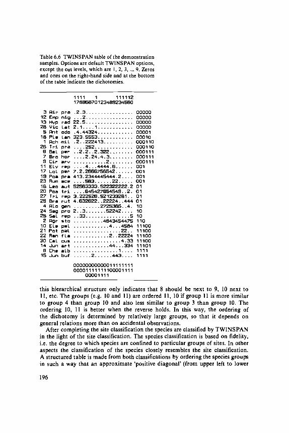
Table 6.6 TWINSPAN table of the demonstrationsamples. Options are default TWINSPAN options,except the cut levels, which are 1, 2, 3, ... 9. Zerosand ones on the right-hand side and at the bottomof the table indicate the dichotomies.

1111 1 11111217895670123489234560

3 Rir pra .2.3 0000012 Emp nig ... 2 0000013 Hyp rad 22.5 0000028 Vic Lat 2. 1.... 1 000005 Rnt odo .4.44324 0000118 Pie Lan 323.5553 000101 Rch mil .2. .222413 000110

26 Tri pra 252 0001106 Bel per ..2.2..2.322 0001117 Bro hor 2.24.4.3 0001119 Cir arv 2 00011111 Ely rep ....4...4444.6 00117 Lol per 7.2.2666756542 00119 Poa pra 413.2344445444.2 00123 Rum ace .... 563 22 00116 Leo aut 52563333.522322222.2 0120 Poa tri ....645427654549..2. 0127 Tri rep 3.222526.521233261.. 0129 Bra rut 4.632622..22224..444 014 Rio gen 2725385. .4. 1024 Sag pro 2. .3 52242 1025 Sal rep . .33 5 102 Rgr sto 4843454475 11010 Ele pal 4. . .4584 1110021 Pot pal 22. . 1110022 Ran f La 2. .22224 1110030 Cal cus 4.33 1110014 Jun art 44.. .334 111018 Che alb 1 111115 Jun buf 2 443.... 1111

0000000000001111111100001111111100001111

00001111

this hierarchical structure only indicates that 8 should be next to 9, 10 next to11, etc. The groups (e.g. 10 and 11) are ordered 11, 10 if group 11 is more similarto group 4 than group 10 and also less similar to group 3 than group 10. Theordering 10, 11 is better when the reverse holds. In this way, the ordering ofthe dichotomy is determined by relatively large groups, so that it depends ongeneral relations more than on accidental observations.

After completing the site classification the species are classified by TWINSPANin the light of the site classification. The species classification is based on fidelity,i.e. the degree to which species are confined to particular groups of sites. In otheraspects the classification of the species closely resembles the site classification.A structured table is made from both classifications by ordering the species groupsin such a way that an approximate 'positive diagonal' (from upper left to lower

196

right) is formed. A TWINSPAN table of the Dune Meadow example is givenin Table 6.6.

6.4 Non-hierarchical clustering

A non-hierarchical clustering can be constructed by selecting sites to act asan initial point for a cluster and then assigning the other sites to the clusters.The methods vary in details. Gauch (1979) starts picking up a random site andclusters all sites within a specified radius from that site. COMPCLUS, as hisprogram is called (composite clustering), repeats this process until all sites areaccounted for. In a second phase, sites from small clusters are reassigned to largerclusters by specifying a larger radius. Janssen (1975) essentially proposes the sameapproach but picks up the first site from the data as initiating point for the firstcluster. This method is applied in CLUSLA (Louppen & van der Maarel 1979).As soon as a site lies further away from the first site than specified by the radius,this site is the initiating point for the next cluster. Subsequent sites are comparedto all previously formed clusters. In this way there is a strong dependence onthe sequence in which the sites enter the classification. A second step in CLUSLAis introduced to reallocate the sites to the 'best' cluster. This is done by comparingall sites with all clusters: if they are more similar to another cluster then to theirparent cluster at that moment, they are placed in the cluster to which they aremost similar. In contrast to COMPCLUS, not only within-cluster homogeneity,but also between cluster distances are used by CLUSLA. A method combiningthe benefits of both methods is used in FLEXCLUS (van Tongeren 1986). Fromthe total set of sites a certain number is selected at random or indicated by theuser. All other sites are assigned to the nearest of the set. By relocation untilstability is reached, a better clustering is achieved. Outliers are removed by reductionof the radius of the clusters afterwards. Variations of these methods are numerous;others have been presented by, for example, Benzecri (1973), Salton & Wong(1978) and Swain (1978).

Although hierarchical clustering has the advantage over non-hierarchical clus-tering that between-group relations are expressed in the classification, there isno guarantee that each level of the hierarchy is optimal. A combination ofhierarchical and non-hierarchical methods can be made by allowing sites to berelocated, to improve clustering. Since clusters change by relocations, this canbe repeated in an iterative process until no further changes occur.

If there is a clear group structure at any level of the hierarchy, no relocationswill be made. An example of such a method is relocative centroid sorting. Thismethod is demonstrated in Figure 6.17. Because of the possibility of relocations,a dendrogram cannot be constructed. By using relocative centroid sorting in aslightly different way - assigning each site to a cluster at random or by a sub-optimal, quick method - as shown in Figure 6.17, computing time can be savedbecause computation of a site-by-site (dis)similarity matrix can be replaced bycomputation of a site-by-cluster matrix. This is used in the table rearrangementprogram TABORD (van der Maarel et al. 1978), and also in CLUSLA (Louppen& van der Maarel 1979) and FLEXCLUS (van Tongeren 1986).

197

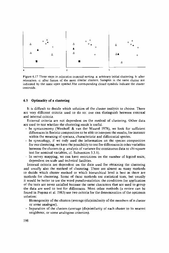
AA

Figure 6.17 Three steps in relocative centroid sorting, a: arbitrary initial clustering, b: afterrelocation, c: after fusion of the most similar clusters. Samples in the same cluster areindicated by the same open symbol.The corresponding closed symbols indicate the clustercentroids.

6.5 Optimality of a clustering

It is difficult to decide which solution of the cluster analysis to choose. Thereare very different criteria used to do so: one can distinguish between externaland internal criteria.

External criteria are not dependent on the method of clustering. Other dataare used to test whether the clustering result is useful.- In syntaxonomy (Westhoff & van der Maarel 1978), we look for sufficient

differences in floristic composition to be able to interpret the results, for instancewithin the meaning of syntaxa, characteristic and differential species.

- In synecology, if we only used the information on the species compositionfor our clustering, we have the possibility to test for differences in other variablesbetween the clusters (e.g. analysis of variance for continuous data or chi-squaretest for nominal variables, cf. Subsection 3.3.1).

- In survey mapping, we can have restrictions on the number of legend units,dependent on scale and technical facilities.

Internal criteria are dependent on the data used for obtaining the clusteringand usually also the method of clustering. There are almost as many methodsto decide which cluster method or which hierarchical level is best as there aremethods for clustering. Some of these methods use statistical tests, but usuallyit would be better to use the word pseudo-statistics: the conditions for applicationof the tests are never satisfied because the same characters that are used to groupthe data are used to test for differences. Most other methods (a review can befound in Popma et al. 1983) use two criteria for the determination of the optimumsolution:

- Homogeneity of the clusters (average (dis)similarity of the members of a clusteror some analogue).

- Separation of the clusters (average (dis)similarity of each cluster to its nearestneighbour, or some analogous criterion).

198

There are many possible definitions of homogeneity and separation of clusters,and each definition might indicate another clustering as the best one. The useof methods to determine the optimum clustering should therefore be restrictedto evaluation of subsequent steps in one type of analysis (Hogeweg 1976; Popmaet al. 1983).

6.6 Presentation of the results

Results of a classification can be presented in different ways. We have alreadymentioned:- the species-by-sites table, giving as much information as possible on all separate

sites and species abundances. In vegetation science, additional environmentalinformation and information on the number of species in a site is usuallyprovided in the head of the table.

- The dendrogram, a representation in which the hierarchical structure of thesite groups is expressed.

When there are many sites, a species-by-sites table becomes quite large andit is not very easy to interpret the table. This is the reason for the constructionof a so-called synoptical table. A synoptical table summarizes the results for eachcluster. Classical synoptical tables in the Braun-Blanquet school of vegetationscience present a presence class and minimum and maximum values for cover/abundance in each vegetation type for all species. Table 8.3 is an example ofsuch a table. In Table 8.3 the presence classes I to V represent within clusterspecies frequencies (0-20, 20-40, 40-60, 60-80, 80-100%, respectively). Many otherways of presenting the summarized data in a synoptical table are possible. Forexample, one can form cross-tabulations of species groups by clusters, or insteadof presence class and minimum and maximum scores, average values and standarddeviations can be entered into the table.

A dendrogram and a species-by-sites table cannot be used for presentation inmore than one dimension. Therefore it can be very useful to present the resultsof the classification in an ordination diagram of the same set of sites. In sucha diagram, more complex relations with the environment can be clearly elucidated(cf. Figure 8.7).

6.7 Relation between community types and environment

The relation between community types as they are defined by cluster analysison the basis of species data and their environment can be explored in severalways. A hierarchical classification can be evaluated at each level: at each dichotomy,a test can be done for differences between the two groups or all clusters at acertain level are evaluated simultaneously. In a non-hierarchical classification weare restricted to simultaneous comparison of all resulting clusters.The range ofmethods goes from exploratory analysis (Subsection 6.7.1) to statistical tests ofsignificance (Subsection 6.7.2).

199

Table 6.7 FLEXCLUS table, similarity ratio, centroid sorting with relocations. Sample 1,which formed a separate cluster, is added to the second cluster by hand. Environmental dataare summarized and added to the table.

Sites:

Leo autBra rutTri repRgr stoRch milRnt odoPla lanPoa praLoL perBel perEly repAlo genPoa triSag proJun bufJun artCal cusEle palRan fLaRir praBro horHyp radPot palRum acze5al repTri praVic latChe albCir arvEmp nig

11 1 1179617085

2635335339422622532622

2 2 24 2443 24 42 5353351 344432676622

2224

4 54 63 2

2324 2

25 2

6 3 53 35 2 22 11

2

123489

522322222521234843

13

44544756423224444 627253276545

5224

•44

42

4 3

2

2

Environmental parameters

Dept R1means.d.% HF% NM

Moisturecl 1cl 2cl 3cl 4cl 5

ManurecL 1cl 2cL 3cL 4

4.01.1

3838

*******

********

3,60.6330

**

**

******

1123

4543245

2

85494241

2

2

11124560

4475444614475

42

4 'J'J45842224

22

5

5.90.100

**

*

7.53.6075

****

*

200

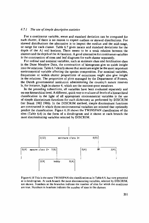
6.7.1 The use of simple descriptive statistics

For a continuous variable, mean and standard deviation can be computed foreach cluster, if there is no reason to expect outliers or skewed distributions. Forskewed distributions the alternative is to inspect the median and the mid-range,or range for each cluster. Table 6.7 gives means and standard deviations for thedepth of the Al soil horizon. There seems to be a weak relation between theclusters and the depth of the A1 horizon. A good alternative for continuous variablesis the construction of stem and leaf diagrams for each cluster separately.

For ordinal and nominal variables, such as moisture class and fertilization classin the Dune Meadow Data, the construction of histograms give us quick insightinto the relations. Table 6.7 clearly shows that moisture might be the most importantenvironmental variable affecting the species composition. For nominal variables,frequencies or within cluster proportions of occurrence might also give insightin the relations. The proportion of plots managed by the Department of Forests,the Dutch governmental institution administering the country's nature reservesis, for instance, high in cluster 4, which are the nutrient-poor meadows.

In the preceding subsections, all variables have been evaluated separately andon one hierarchical level. A different, quick way to evaluate all levels of a hierarchicalclassification in the light of all appropriate environmental variables is the useof simple discriminant functions for each dichotomy as performed by DISCRIM(ter Braak 1982 1986). In the DISCRIM method, simple discriminant functionsare constructed in which those environmental variables are selected that optimallypredict the classification. Figuie 6.18 shows the TWINSPAN classification of thesites (Table 6.6) in the form of a dendrogram and it shows at each branch themost discriminating variables selected by DISCRIM.

1(12) moisture class 3+ 8(8)

0(4) manure class 2+ 7(8) 0(4) NM 3(4)

3(4) hobby 0(4)

Figure 6.18 This is the same TWINSPAN site classification as in Table 6.6, but now presentedas a dendrogram. At each branch the most discriminating variables, selected by DISCRIM,are shown. Numbers at the branches indicate the number of sites for which the conditionsare true. Numbers in brackets indicate the number of sites in the clusters.

201

6.7.2 The use of tests of significance

Tests of significance are introduced in Chapter 3, Section 3.2. To test whetherany environmental variable might be controlling the species composition (or mightbe controlled by the species composition, or simply related to the speciescomposition) in the communities, we take as null hypothesis that the speciescomposition is independent from the environmental variable. Rejecting the nullhypothesis indicates that the environmental variable is related to the speciescomposition of our community types in some way or another.

Analysis of variance

Analysis of variance is explained in Subsection 3.2.1. It can be used to detectrelations between community types and continuous environmental variables. Thesystematic part consists of the expected values of the environmental variable,one for each community type and the error part is the variation in the valueswithin each community type. Analysis of variance is based on the normaldistribution. Therefore environmental variables must often be transformed, e.g.by using the logarithm of their values (see Subsection 2.4.4).

Chi-square test

Subsection 3.3.1 describes the chi-square test for r x k contingency tables. Thechi-square test is used to test the null hypothesis: that a nominal environmentalvariable is not related to the community types. Care should be taken if the numbersof data are small or if the frequency of occurrence of the nominal variable islow (see Subsection 3.3.1).

The rank sum test for two independent samples

Analysis of variance and the / test (cf. Subsection 3.2.1) are not very resistantto outliers, because they are very much affected by gross errors in the observations.An alternative is to use a distribution-free method, like the rank sum test fortwo independent samples. As its name indicates, this test, developed by Wilcoxon,but also known as the Mann-Whitney test, can be used to test for differencesbetween two groups. The test is described below.

All observations in both groups are put into a single array in increasing order(indicating also from which group they are) and rank numbers are given to theobservations (the smallest observation has rank number 1). Tied observations(equal values) are given their average rank number. For equal sample sizes thesmallest sum of rank numbers of both groups is directly referred to a table forthe Mann-Whitney test. For unequal sample sizes the sum of the rank numbersis computed for the smallest sample (T{). A second T(T2) is computed:

202

where n] and n2 are the sizes of the smaller and the larger sample, respectively.

The test criterion T is the smaller of Tx and T2. For sample sizes outside thelimits of the table, an approximate normal deviate Z is referred to the tablesof the normal distribution to obtain the significance probability P:

Z = ( | u - T | - 0 . 5 ) / a

where |i = («,-f«2+l)/2 and a =

With this test two small groups (minimum sizes of 4 and 4, 3 and 5 or 2 and8) can be compared without any assumption on the distribution of the envir-onmental variable. For further details on this test and other tests of significancerefer to a statistical handbook (e.g. Snedecor & Cochran 1980).

6.8 Bibliography

Scientific classification of communities can be traced back in history to vonHumboldt (1807): he used associations of plants to define community types. Jaccard(1912) took the first step in the direction of multivariate analysis by the developmentof his index of similarity. Many years later he was followed by Sorensen (1948),who developed his 'method of establishing groups of equal amplitude in plantsociology' based on similarity of species content. The increasing access scientistshave had to computers over the last thirty years has led to rapid developmentsin multivariate methods. An early work that is devoted to the use of multivariatemethods in taxonomy is a book written by Sokal & Sneath (1963). In the latesixties, and 1970s there was a rapid increase in the use of cluster analysis (andordination) by ecologists. Pielou (1969), Goodall (1970) and Williams (1976a)give a theoretical background to these methods.

Numerical classification in the phytosociological context is elucidated by Goodall(1973) and Mueller-Dombois & Ellenberg(1974). Everitt (1980) and Dunn & Everitt(1982) are more recent introductions to numerical taxonomy. Gauch (1982) givesan introduction to classification of communities and mentions many applicationsof cluster analysis.

203

6.9 Exercises

Exercise 6.1 Single-linkage clustering with Jaccard similarity

Exercise 6.1a Compute the Jaccard similarities for the sites in the artificial species-by-site table given below. Since the similarities are symmetrical and the diagonalelements all equal 1, you should only compute the elements below the diagonalof the site-by-site similarity matrix (cf. Exercise 6.1c for the species).

Site

Species ABCDEFG

1

12

1

2

4

1131

3

1

1

13

4

1

41

5

2

1

1

6

2

53

Exercise 6.1b Perform single-linkage clustering for the sites.

Exercise 6.1c The species similarities are:

BCDEFG

A

000.600.400.600.60

B

000.330.250

C

0.25000.25

D

0.170.331.0

E

0.0.

7517

F

0.33

Perform single-linkage clustering for the species.

Exercise 6.1d Rearrange the sites and the species to represent the hierarchicalstructure. Try also to obtain the best possible ordering.

204

Exercise 6.2 Complete-linkage clustering with percentage similarity

Exercise 6.2a Compute the missing elements (denoted by *) of the site-by-sitesimilarity matrix (percentage similarity) for the table of Exercise 6.1a.

23456

1

29400

500

2

*255860

3

1760*

4

*63

5

29

Exercise 6.2b Perform complete-linkage clustering for all sites.

Exercise 6.3 Single-linkage clustering with Euclidean Distance

Exercise 6.3a Compute the missing elements (denoted by*) of the site-by-siteEuclidean Distance matrix for the table of Exercise 6.1a.

23456

1

5.3*4.92.56.3

2

4.25.73.84.7

3

526

.3

.5

.3

4 5

4.92.5 *

Exercise 6.3b Perform single linkage and try to find out why the result is sodifferent from Exercise 6.1.

Exercise 6.4 Divisive clustering

This exercise is a demonstration of a simple classification procedure using adivisive strategy with iterative character weighting (this procedure is different fromthe procedures used in TWINSPAN and by Hogeweg (1976)). The species-by-sites table of Exercise 6.1 is used here too.

Step a Divide the sites in two groups, a positive and a negative one. You maychoose a random division or monothetic division based on the presence of onespecies. In the solution we intially place Sites 1,3 and 6 in the negative groupand Sites 5,2 and 4 in the positive group.

Step b Compute the sum of abundances for each species for both sides of thedichotomy (SPOS for the positive scores, SNEG for the negative scores).

205

Step c Compute a preference score for each species: pref = (SPOS—SNEG)/(SPOS+SNEG).

Step d Compute a weighted sum (or weighted average) of the species abundancesfor each site.

Step e Find maximum and minimum site score (MAX and MIN) and the midpointof the site scores (MID = (MAX+MIN)/2).

Step f Assign all sites with a score less than the midpoint to the 'negative' groupand all the other sites to the 'positive' group.

Step g Repeat steps b-f until the division is stable.

Step h Repeat steps a-g for each subgroup.

Exercice 6.5 Cluster interpretation with nominal environmental data

Do the chi-square test for moisture classes 1 and 2 combined, and 3, 4, and5 combined, for:

Exercise 6.5a The first division of TWINSPAN (Table 6.6)

Exercise 6.5b The first three clusters of Table 6.7 combined and the last cluster(highest hierarchical level). What is your null-hypothesis? Has it to be rejectedor not? Is it correct to use the chi-square test in this case?

Exercise 6.6. Cluster interpretation with ordinal environmental data

Perform Wilcoxon's test for 'Depth of AT for the first division of TWINSPAN(Table 6.6).

206

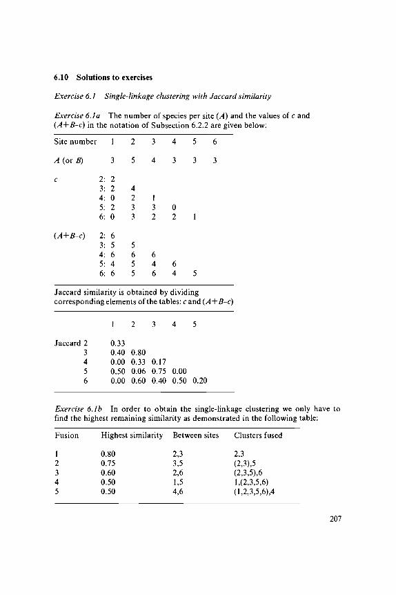
6.10 Solutions to exercises

Exercise 6.1 Single-linkage clustering with Jaccard similarity

Exercise 6.1a The number of species per site (A) and the values of c and(A+B-c) in the notation of Subsection 6.2.2 are given below:

Site number 1

A (or B)

c

{A+B-c)

3

2: 23: 24: 05: 26: 0

2: 63: 54: 65: 46: 6

Jaccard similarity is <

2

5

4233

5655

3

4

132

646

Dbtained by

4

3

02

64

5 6

3 3

1

5

dividingcorresponding elements of the tables: c and (A-\~B-c)

Jaccard 23456

1

0.330.400.000.500.00

2

0.800.330.060.60

3

0.170.750.40

4

0.000.50

5

0.20

Exercise 6.1b In order to obtain the single-linkage clustering we only have tofind the highest remaining similarity as demonstrated in the following table:

Fusion

12345

Highest similarity

0.800.750.600.500.50

Between sites

2,33,52,61,54,6

Clusters fused

2,3(2,3),5(2,3,5),61,(2,3,5,6)(1,2,3,5,6),4

207

Exercise 6.1c

Fusion

123456

Highest similarity

1.00.750.600.600.330.25

Between species

D,GE,FA,DA,FB,EC,D

Clusters fused

D,GE,FA,(D,G)(A,D,G),(E,F)(A,D,E,F,G),B(A,B,D,E,F,G),C

Exercise 6. Id The hierarchy can be represented in a dendrogram in which eachdichotomy can be swivelled. In order to obtain the best possible ordering eachsite is placed next to its nearest neighbour.

2 next to 3:5 next to 3:6 next to 2:1 next to 5:4 next to 6:or the reverse

226641

332265

53323

5532

156

14

If we use the same procedure for the species, there is a problem for species C.

D next to G: D G or G DE next to F: E F or F EA next to D: A D G or G D AA next to F i E F A D G o r G D A F EB next to E: B E F A D G o r G D A F E BC between A and D is not a good solution because A resembles D much morethan C does.C next to G is better, but still there are two possibilities, C between D and Gor C at the end. Because C resembles A less than D and G do, C is placedat the end of the ordering:B E F A D G C o r C G D A F E B

The rearranged table:

cGDAFEB

1112

5

112

3

3111

2

11431

6

235

4

141

208

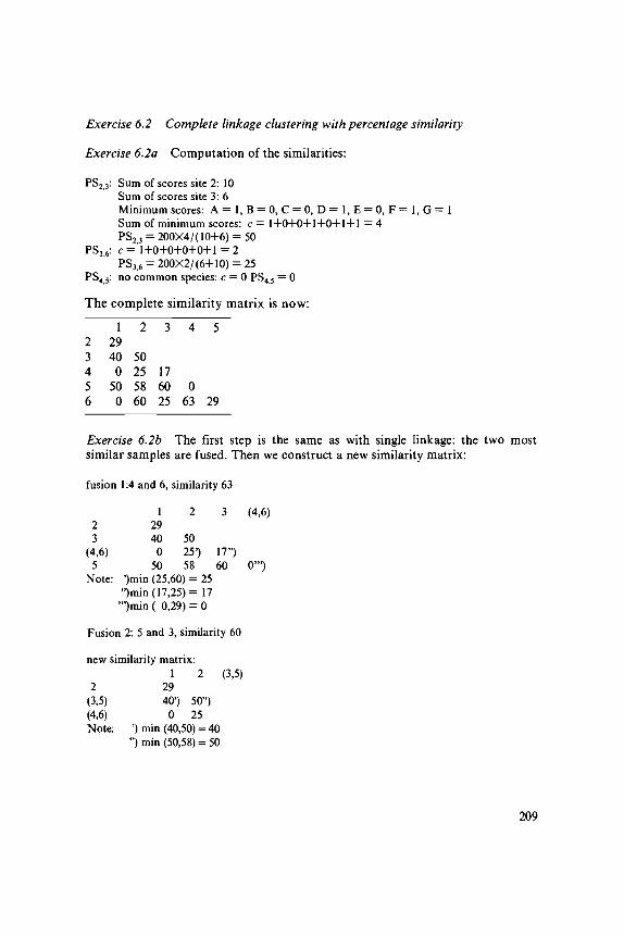
Exercise 6.2 Complete linkage clustering with percentage similarity

Exercise 6.2a Computation of the similarities:

PS2 3: Sum of scores site 2: 10Sum of scores site 3: 6Minimum scores: A = 1, B = 0, C = 0, D = 1, E = 0, F = 1, G = 1Sum of minimum scores: c = 1+0+0+1+0+1+1 = 4PS23 = 200X4/(10+6) = 50

PS36: c =1+0+0+0+0+1 = 2PS3?6 = 200X2/(6+10) = 25

PS4 5: no common species: c = 0 PS4 5 = 0

The complete similarity matrix is now:

23456

129400500

2

50255860

3

176025

4

063

5

29

Exercise 6.2b The first step is the same as with single linkage: the two mostsimilar samples are fused. Then we construct a new similarity matrix:

fusion 1:4 and 6, similarity 63

1 2 3 (4,6)2 293 40 50

(4,6) 0 25') 17")5 50 58 60 0'")

Note: ')min (25,60) = 25")min (17,25) = 17'")min ( 0,29) = 0

Fusion 2: 5 and 3, similarity 60

new similarity matrix:1 2 (3,5)

2 29(3.5) 40') 50")(4.6) 0 25Note: ') min (40,50) = 40

") min (50,58) = 50

209

Fusion 3: 2 and (3,5), similarity 50

new similarity matrix:1 (2,3,5)

(2,3,5) 29(4,6) 0 0

Fusion 4: (2,3,5) and 1, similarity 29

last fusion: (1,2,3,5) and (4,6), similarity 0

Exercise 6.3 Single-linkage clustering with Euclidean Distance

Exercise 6.3 a

ED, 3 = [(0-l)2+(0-0)2+(l-0)2+(2-l)2+ (0-0)2 +(0-l)2+(l-3)2]1/2

ED5 6 = [(2-0)2+(0-0)2+(0-5)2+(0-3)2+ (1-0' !/2

Exercise 6.3b Instead of looking for the highest similarity values, we look forthe lowest dissimilarity values.

Fusion

12345

Dissimilarity

2.52.52.54.24.7

Between sites

1,53,54,62,32,6

Clusters fused

1,5(1,5),34,6(1,3,5),2(1,2,3,5),(4,6)

Now Sites 4 and 6 group together because of the dominance of Species E. Sites2 and 3 are more different and fuse therefore later, because of the differentabundances for Species A, F and G. Sites 1 and 5 are fused first, because oftheir low species abundances, and so on.

210

Exercise 6.4 Divisive clustering

Steps a-g The species-by-sites table (Table 6.8) is rearranged according to thesolution from Exercise 6.1.

Table 6.8 Species-by-sites table rearranged according to the solution for Exercise 6.1, withSPOS, SNEG and PREF computed in Steps b and c of the iteration algorithm of Exercise 6.4.

11 12 1

2

3111

11431

235

141

step 1

SPOS

0226451

b

SNEG

1433450

step 1 c

PREF

-1-0.33-0.20

0.33001

step 2

SPOS

02287

101

b

SNEG

1431100

step 2 c

PREF

-1-0.33-0.200.780.7511

step 3

SPOS

01167

101

b

SNEG

1543100

step 3 c

PREF

-1-0.67-0.750.330.75

11

Step la Initial choice: Sites 1, 3 and 6 in the negative group; Sites 2, 4 and 5 in thepositive group.

Step lb- lc See Table 6.8.Step Id For Sites 1-6 the weighted sums of the preference scores are —1.73, 0.79,

-0.86, 1, 0.13 and 0.66, respectively.Step le MID = (-1.73 + l)/2 = -0.36.Step If Sites 1 and 3 in the negative group; the other sites in the positive group.Step 2b-2c See Table 6.8.Step2d For Sites 1-6 the weighted sums are -1.73, 5.84, 0.34, 5.75, 1.03 and 8.81,

respectively.Step 2e MID = (-1.73 + 8.81)/2 = 3.56.Step 2f Sites 1, 3 and 5 in the negative group; the other sites in the positive group.Step 3b-3c See Table 6.8.Step 3d For Sites 1-6 the weighted sums are -3.17, 2.15, -1.68, 5.75, -0.76 and 7.91,

respectively.Step 3e MID = (-3.17 + 7.91)/2 = 2.37.Step 3f Same as Step 2f, so the classification is stable now.

Step h This is solved in essentially the same way for further subdivisions.

Exercise 6.5 Cluster interpretation with nominal environmental dataWe start by making two-way cross-tabulations of the observed frequencies (o):

TWINSPAN (Table 6.6) FLEXCLUS (Table 6.7)

Cluster number:Moisture class: 1+2

3+4+5Total:

0111

12

1088

total119

20

1+2+3115

16

4044

total119

20

211

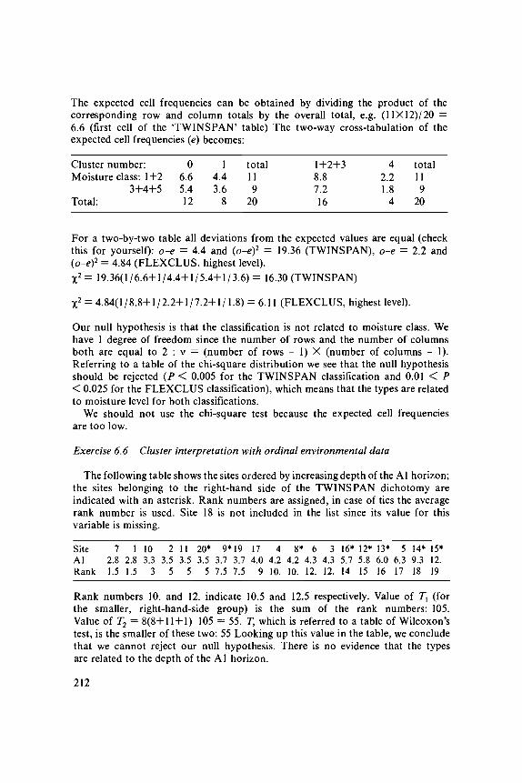
The expected cell frequencies can be obtained by dividing the product of thecorresponding row and column totals by the overall total, e.g. (11X12)/2O =6.6 (first cell of the TWINSPAN' table) The two-way cross-tabulation of theexpected cell frequencies (e) becomes:

Cluster number:Moisture class: 1+2

3+4+5Total:

06.65.412

14.43.6

8

total119

20

1+2+38.87.216

42.21.8

4

total119

20

For a two-by-two table all deviations from the expected values are equal (checkthis for yourself): o-e = 4.4 and (o-e)2 = 19.36 (TWINSPAN), o-e = 2.2 and(o-e)2 = 4.84 (FLEXCLUS, highest level).X2= 19.36(1/6.6+1/4.4+1/5.4+1/3.6)= 16.30 (TWINSPAN)

X2 = 4.84(1/8.8+1/2.2+1/7.2+1/1.8) = 6.11 (FLEXCLUS, highest level).

Our null hypothesis is that the classification is not related to moisture class. Wehave 1 degree of freedom since the number of rows and the number of columnsboth are equal to 2 : v = (number of rows - 1) X (number of columns - 1).Referring to a table of the chi-square distribution we see that the null hypothesisshould be rejected (P < 0.005 for the TWINSPAN classification and 0.01 < P< 0.025 for the FLEXCLUS classification), which means that the types are relatedto moisture level for both classifications.

We should not use the chi-square test because the expected cell frequenciesare too low.

Exercise 6.6 Cluster interpretation with ordinal environmental data

The following table shows the sites ordered by increasing depth of the Al horizon;the sites belonging to the right-hand side of the TWINSPAN dichotomy areindicated with an asterisk. Rank numbers are assigned, in case of ties the averagerank number is used. Site 18 is not included in the list since its value for thisvariable is missing.

Site 7 1 10 2 11 20* 9*19 17 4 8* 6 3 16* 12* 13* 5 14* 15*Al 2.8 2.8 3.3 3.5 3.5 3.5 3.7 3.7 4.0 4.2 4.2 4.3 4.3 5.7 5.8 6.0 6.3 9.3 12.Rank 1.5 1.5 3 5 5 5 7.5 7.5 9 10. 10. 12. 12. 14 15 16 17 18 19

Rank numbers 10. and 12. indicate 10.5 and 12.5 respectively. Value of T{ (forthe smaller, right-hand-side group) is the sum of the rank numbers: 105.Value of T2 = 8(8+1 l+l)-105 = 55. T, which is referred to a table of Wilcoxon'stest, is the smaller of these two: 55 Looking up this value in the table, we concludethat we cannot reject our null hypothesis. There is no evidence that the typesare related to the depth of the Al horizon.

212