Cross-Selling the Right Product to the Right Customer at the Right Time

Shibo Li1 Kelley School of Business

Indiana University 1309 E. 10th Street

Bloomington, IN 47405 Phone: 812-855-9015

Fax: 812-855-6440 Email: shili@indiana.edu

Baohong Sun

Tepper School of Business Carnegie Mellon University

5000 Forbes Avenue Pittsburgh, PA15213

Tel: 412-268-6903 Fax: 412-268-7357

Email: bsun@andrew.cmu.edu

and

Alan L. Montgomery Tepper School of Business Carnegie Mellon University

5000 Forbes Avenue Pittsburgh, PA15213

Tel: 412-268-4562 Fax: 412-268-7357

Email: alm3@andrew.cmu.edu

January 2009

Revised, May 2010 Second Revision, September 2010 Third Revision, November 2010

1 Shibo Li is an Assistant Professor of Marketing at Indiana University. Baohong Sun is the Carnegie Bosch Professor of Marketing and Alan L. Montgomery is an Associate Professor at Carnegie Mellon University. We also thank our project sponsor—who wishes to remain anonymous—for providing the data used in this project. All opinions expressed in this paper are our own and do not reflect those of our project sponsor. We would like to thank the Customer Relationship Management Center at Duke University for its generous financial support.

Cross-Selling the Right Product to the Right Customer at the Right Time

Abstract

Firms are challenged to improve the effectiveness of cross-selling campaigns. In this research, we propose a customer-response model that recognizes the evolvement of customer demand for various products, the possible multi-faceted roles of cross-selling solicitations for promotion, advertising, and education, and customer heterogeneous preference for communication channels. We formulate cross-selling campaigns as solutions to a stochastic dynamic programming problem in which the firm’s goal is to maximize the long-term profit of its existing customers while taking into account the development of customer demand over time and the multi-stage role of cross-selling promotion. The model yields optimal cross-selling strategies about how to introduce the right product to the right customer at the right time using the right communication channel. Applying the model to panel data with cross-selling solicitations provided by a national bank, we demonstrate that households have different preferences and responsiveness to cross-selling solicitations. Other than generating immediate sales, cross-selling solicitations also help households move faster along the financial continuum (educational role) and build up good will (advertising role). We show that the suggested cross-selling solicitations are more customized and dynamic and significantly improve over the currently adopted campaign-centric solicitations.

Keywords: cross-selling, customer relationship management, customer long-term profit contribution, dynamic structural model, development of customer demand, multi-channel communication

- 1 -

1. Introduction

Cross-selling is the practice of selling an additional product or service to an existing

customer. It ranks as a top strategic priority for many industries including financial services,

insurance, health care, accounting, telecommunications, airlines, and retailing. Despite the increasing

investment in cross-selling programs, firms find that these million-dollar marketing campaigns are

not profitable (Authers 1998; Business Wire 2000; Rosen 2004). The average response rate as

measured by a customer purchase within three months after a cross-selling campaign is about 2

percent (Business Wire 2000; Smith 2006). A managerial challenge is to improve the response rates

of a cross-selling campaign while avoiding the targeting of customers with irrelevant messages.

Most current cross-selling campaigns are designed with this orientation: “let’s find the customers

who are most likely to respond.” Firms begin cross-selling campaigns by setting a time schedule (e.g., mail

the promotional material in one month) and then select a communication channel (e.g., phone, email,

or mail) for this campaign. Analysts then develop a customer-response model with the purchase

decision as a dependent variable and product ownership and customer demographics as explanatory

variables. Finally, upon estimation of the customer-response model, the expected profit is

computed, and firms schedule all customers with positive expected profits to receive the promotion.

If the firm has to heed a budget constraint, it will only solicit the most profitable customers. We

refer to this process as campaign-oriented cross-selling.

We argue that an improved customer-centric orientation for cross-selling is: “how do we

introduce the right product to the right customer at the right time using the right communication channel to ensure long-

term success.” Conceptually, customer demand for financial services depends upon the customer’s

evolving financial maturity (Kamakura, Ramaswami, and Srivastava 1991; Li, Sun, and Wilcox 2005).

Thus, each individual customer’s preferences and responsiveness to cross-selling solicitations may

change over time and the marketer has to track and anticipate these changes (Netzer, Lattin, and

- 2 -

Srinivasan 2008). In addition, cross-selling solicitations may provide more than just a promotional

incentive that immediately stimulates purchase. Cross-selling can create enduring relationships

between a customer and the firm by serving as a general advertisement for the brand, a signal of

quality, and to educate consumers about the scope of product offerings and how various products

meet their long-term financial needs. Ultimately this requires the marketer to have a long term view

and generate dynamic solicitations in accordance with the customer’s evolving financial status and

preferences in order to maximize the long-term financial payoff (Sun, Li, and Zhou 2006).

The focus of our research is to take up this challenge and understand the many roles of

solicitations within a cross-selling campaign, how it interacts with customer purchase decisions, and

to explore how cross-selling can be improved. More specifically, we address the following open

research questions: How do cross-selling solicitations interact with customer decision process about

purchases of financial products? Do cross-selling solicitations have long-term effects other than

generating immediate purchase? If yes, how can we decompose the short- and long-term

effectiveness of cross-selling campaigns? Do customers differ in their preference for

communication channels? How should a firm best utilize the long-term role of cross-selling

solicitations when making cross-selling solicitation decisions?

We develop a multivariate customer-response model with hidden Markov transition states to

statistically capture the possibility that customer demand for various financial products is governed

by evolving latent financial states, during which customers have different preference priorities as

well as responsiveness to cross-selling solicitations for various financial products. We capture long-

term effects of solicitations by allowing cross-selling to change the speed of customer movement

along the financial maturity continuum. Across-customer heterogeneity is captured through a

hierarchical Bayesian framework. We calibrate our model to customer purchase histories provided

by a national bank.

- 3 -

Based on the estimated customer-response parameters, we formulate the bank’s cross-selling

decisions as solutions to a stochastic dynamic programming problem that maximizes customer long-

term profit contribution. This proposed dynamic optimization framework allows us to integrate

intra-customer heterogeneity (the evolving financial states of each customer) and long-term dynamic

effects of cross-selling solicitations. It results in a sequence of solicitations that represent an

integrated multi-step, multi-segment, and multi-channel cross-selling campaign process to optimize

the choice and timing of these messages. We compare our results with current industry practice and

several alternative cross-selling approaches that ignore intra-customer heterogeneity, disregard the

cumulative effects of cross-selling, and make cross-selling decisions myopically. Comparing with

current practice observed in our dataset, our proposed approach improves immediate response rate

by 56 percent, long-term response rate by 149 percent, and long-term profit by 177 percent.

2. Cross-Selling Literature

We summarize previous academic research on cross-selling and customer lifetime value

analysis in Table 1. Existing literature focuses on developing methods to more accurately predict

purchase probabilities for the next product-to-be-purchased, and is useful in supporting campaign-

centric cross-selling or the next product-to-be-cross-sold. Except for Kumar et al (2008a), none of

the existing cross-selling papers use information on cross-selling solicitations and there is little

known about how cross-selling solicitations affect customer purchase decisions in the long term.

Customer lifetime value (CLV) in campaign-oriented cross-selling is usually treated as another

segmentation variable to differentiate profitable customers from unprofitable ones. However, Rust

and Chung (2006) and Rust and Verhoef (2005) point out the problem with this approach is that the

bank’s intervention changes a customer’s future purchase probabilities.

[Insert Table 1 About Here]

- 4 -

Our paper contributes to the existing literature on cross-selling in the following ways. First,

we directly observe the cross-selling solicitations (or promotions) made to customers in our

empirical study. Hence ours is the first study that explicitly models how customers dynamically react

to cross-selling solicitations and measures the effectiveness of cross-selling solicitations in the short

and long runs. Second, we relax the strong assumption that customer responsiveness to solicitations

is fixed over time and allows the responsiveness to solicitations to change over time. The evolving

state structure allows us to investigate how effectiveness of solicitations cross-selling different

products varies with customer financial states or communication channels. Third, we recognize and

model the long-term effects of solicitation in the customer response model (which we refer to as the

educational and advertising roles). These effects have been documented by industry reports (Rough

Notes 2010) but not in the academic literature. Fourth and most importantly, we demonstrate that

intra-customer heterogeneity and long-term effects of solicitations require the firm to take a long-

term view and adopt a dynamic programming approach when making solicitation decisions.

3. Data Description

Our data is provided by a national bank that offers a complete line of retail banking services.

The data set consists of monthly account opening and transaction histories, cross-selling solicitations

about the type of product promoted and the communication channels used (i.e., email or postal

mail), and demographic information (compiled by a marketing research firm to which the bank

subscribes) of a randomly selected sample of 4,000 households for 15 financial product groups

during a total of 27 months from November 2003 through January 2006.

We group the 15 products into seven categories: checking, savings, credit cards, lending,

CDs, investment, and others.2 Therefore our purchase variable records when a specific account is

2 Checking includes various types of checking accounts; savings includes money market and savings accounts; credit cards include credit cards and bank cards; lending includes mortgage, term loans and secure credit line; CDs include time

- 5 -

opened. Since there are multiple financial products within a category, repeat purchases are recorded

as a purchase of a financial product (category). For example, a customer with an existing free

checking account opens a second interest checking account. Notice that this is represented in our

data as a purchase. Additionally, our analysis is at the household level that may be made up of many

individuals. Repeat purchases of similar products can be purchased by or for other household

members. In short, we do not distinguish between new products within a category, repeat purchases

by the same individual, or new purchases by other household members. Third, it is rare that

customers make more than one purchase in a category within a single month, so we focus on an

indicator of purchase within the category and not the number of items purchased.

Our calibration sample consists of 2,000 randomly selected households that received a total

of 12,590 solicitations and made a total of 4,948 purchases during the 27 months. We have a cross-

sectional validation sample with another 2,000 randomly selected households that were contacted

12,797 times and made 5,038 purchases during the same 27 months. Additionally, for cross-time

validation we use the first 26 months of these 4,000 households for estimation and retain the final

month for a holdout sample.

[Insert Table 2 about here]

Table 2 gives a brief description of the variables this paper uses for the whole sample. The

households have average total assets of $97,243.4 as estimated by a marketing research company.

The variable COMP measures the share-of-wallet or percentage of customer assets that are allocated

to other financial institutions. This variable is just an estimate by the marketing research company

and is a static measure of competition from other financial institutions. We observe the number of

deposits or CDs; Investment include annuity, trusts and security investments; and Other includes safe deposit box and other services. This classification follows the practice of the bank and helps us avoid estimation issues related to data scarcity. We acknowledge that this is a simplification, but it is an accepted practice (Kamakura, Ramaswami, and Srivastava 1991; Li, Sun and Wilcox 2005; Edwards and Allenby 2003) and we believe it preserves the basic structure of the problem. The exercise of aggregating both across similar products and household members are related to the data we are provided with. However, the proposed model can be applied to data without data aggregation.

- 6 -

solicitations sent to the average household during the 27 months is 6.35. The bank deliberately

avoids trying to overwhelm its customers with solicitations and limits its marketing activities to

around one solicitation per quarter. The bank provides us with the profit information for each

household and every account. These profit margins are calculated using full absorption accounting

based upon the customer’s usage of the bank’s services. The average profit margin per account per

month is $14.71. We also learn from bank managers that the average cross-selling solicitation costs

about $0.50 and $0.05 per message for postal and email, respectively.

4. Customer-Response Model

We observe the set of financial products and services a household purchases and the cross-

selling campaign messages it receives each month. The bank needs to evaluate how the cross-selling

solicitations interact with customer decision process, what are the short-term and long-term

consequences of these campaign messages on household cross-buying decisions, and predict when

customers will open a new account. The core of our model is a multivariate probit model that

predicts whether a household will decide to open a new account in a given month (§4.1). The

covariates within the probit model reflect how the customer’s decisions are influenced by cross-

selling efforts of the bank, as well as the household’s characteristics. The parameters of this probit

model depend upon a latent financial state for each customer that we estimate (§4.2). This latent

state is time dependent, and its dynamics explain how a customer’s financial status can change and

influence a customer’s response to marketing efforts. The hierarchical specification of our model

relates the probit parameters to a household’s characteristics (§4.3). To optimize consumer response

to cross-selling efforts we first specify the long-term profit for a customer (§5.1) and then show how

to dynamically optimize this objective (§5.2).

- 7 -

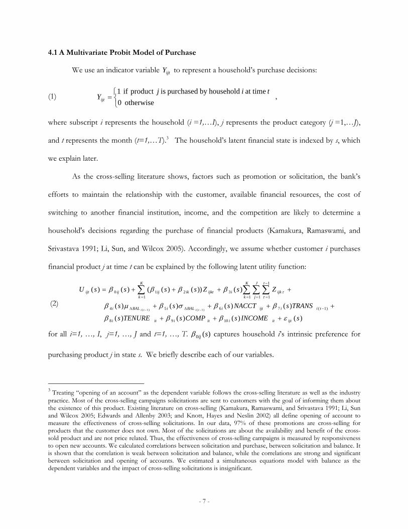
4.1 A Multivariate Probit Model of Purchase

We use an indicator variable ijtY to represent a household’s purchase decisions:

(1)

otherwise 0

at time householdby purchased is product if 1 tijYijt

,

where subscript i represents the household (i =1,…I), j represents the product category (j =1,…J),

and t represents the month (t=1,…T).3 The household’s latent financial state is indexed by s, which

we explain later.

As the cross-selling literature shows, factors such as promotion or solicitation, the bank’s

efforts to maintain the relationship with the customer, available financial resources, the cost of

switching to another financial institution, income, and the competition are likely to determine a

household's decisions regarding the purchase of financial products (Kamakura, Ramaswami, and

Srivastava 1991; Li, Sun, and Wilcox 2005). Accordingly, we assume whether customer i purchases

financial product j at time t can be explained by the following latent utility function:

(2)

)()()()(

)()()()(

)())()(()()(

1098

)1(7654

1 1

1

13

1210

)1()1(

sINCOMEsCOMPsTENUREs

TRANSsNACCTsss

ZsZssssU

ijtitiitiiti

tiiijtiBALiBALi

K

k

J

j

t

ijkiijkt

K

kikijijijt

titi

for all i=1, …, I, j=1, …, J and t=1, …, T. )(0 sij captures household i’s intrinsic preference for

purchasing product j in state s. We briefly describe each of our variables.

3 Treating “opening of an account” as the dependent variable follows the cross-selling literature as well as the industry practice. Most of the cross-selling campaigns solicitations are sent to customers with the goal of informing them about the existence of this product. Existing literature on cross-selling (Kamakura, Ramaswami, and Srivastava 1991; Li, Sun and Wilcox 2005; Edwards and Allenby 2003; and Knott, Hayes and Neslin 2002) all define opening of account to measure the effectiveness of cross-selling solicitations. In our data, 97% of these promotions are cross-selling for products that the customer does not own. Most of the solicitations are about the availability and benefit of the cross-sold product and are not price related. Thus, the effectiveness of cross-selling campaigns is measured by responsiveness to open new accounts. We calculated correlations between solicitation and purchase, between solicitation and balance. It is shown that the correlation is weak between solicitation and balance, while the correlations are strong and significant between solicitation and opening of accounts. We estimated a simultaneous equations model with balance as the dependent variables and the impact of cross-selling solicitations is insignificant.

- 8 -

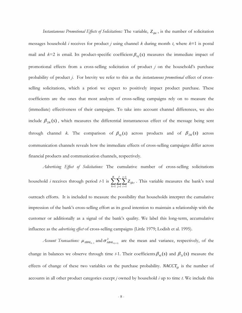
Instantaneous Promotional Effects of Solicitations: The variable, ijktZ , is the number of solicitation

messages household i receives for product j using channel k during month t, where k=1 is postal

mail and k=2 is email. Its product-specific coefficient )(1 sij measures the immediate impact of

promotional effects from a cross-selling solicitation of product j on the household’s purchase

probability of product j. For brevity we refer to this as the instantaneous promotional effect of cross-

selling solicitations, which a priori we expect to positively impact product purchase. These

coefficients are the ones that most analysts of cross-selling campaigns rely on to measure the

(immediate) effectiveness of their campaigns. To take into account channel differences, we also

include )(2 sik , which measures the differential instantaneous effect of the message being sent

through channel k. The comparison of )(1 sij across products and of )(2 sik across

communication channels reveals how the immediate effects of cross-selling campaigns differ across

financial products and communication channels, respectively.

Advertising Effect of Solicitations: The cumulative number of cross-selling solicitations

household i receives through period t-1 is

K

k

J

j

t

ijkZ1 1

1

1 . This variable measures the bank’s total

outreach efforts. It is included to measure the possibility that households interpret the cumulative

impression of the bank’s cross-selling effort as its good intention to maintain a relationship with the

customer or additionally as a signal of the bank’s quality. We label this long-term, accumulative

influence as the advertising effect of cross-selling campaigns (Little 1979; Lodish et al. 1995).

Account Transactions: 1 itBAL and 2

)1( tiBAL are the mean and variance, respectively, of the

change in balances we observe through time t-1. Their coefficients )(4 si and )(5 si measure the

effects of change of these two variables on the purchase probability. ijtNACCT is the number of

accounts in all other product categories except j owned by household i up to time t. We include this

- 9 -

variable to control for the possibility that the currently owned accounts in other product categories

may compete for financial resources and thus affects the probability of purchasing a new financial

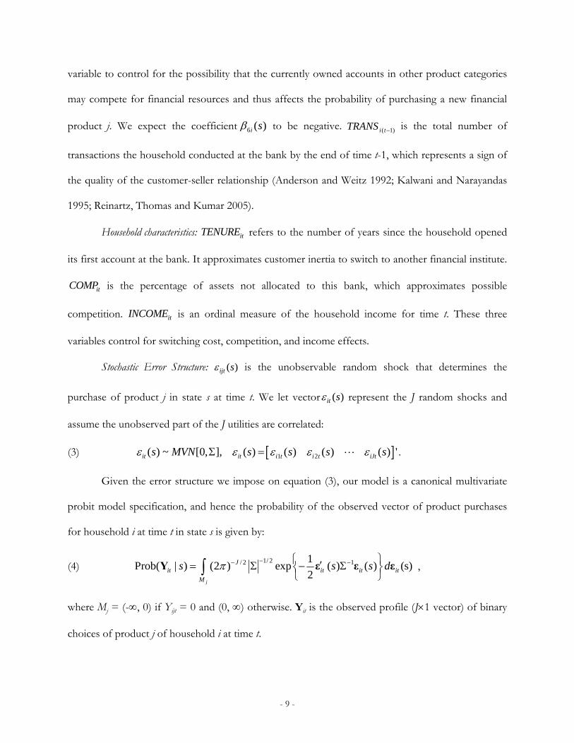
product j. We expect the coefficient 6 ( )i s to be negative. )1( tiTRANS is the total number of

transactions the household conducted at the bank by the end of time t-1, which represents a sign of

the quality of the customer-seller relationship (Anderson and Weitz 1992; Kalwani and Narayandas

1995; Reinartz, Thomas and Kumar 2005).

Household characteristics: itTENURE refers to the number of years since the household opened

its first account at the bank. It approximates customer inertia to switch to another financial institute.

itCOMP is the percentage of assets not allocated to this bank, which approximates possible

competition. itINCOME is an ordinal measure of the household income for time t. These three

variables control for switching cost, competition, and income effects.

Stochastic Error Structure: )(sijt is the unobservable random shock that determines the

purchase of product j in state s at time t. We let vector )(sit represent the J random shocks and

assume the unobserved part of the J utilities are correlated:

(3) 1 2( ) ~ [0, ], ( ) ( ) ( ) ( ) 'it it i t i t iJts MVN s s s s .

Given the error structure we impose on equation (3), our model is a canonical multivariate

probit model specification, and hence the probability of the observed vector of product purchases

for household i at time t in state s is given by:

(4) 1/ 2/ 2 11

Prob( | ) (2 ) exp ( ) ( ) (s) 2

j

Jit it it it

M

s s s d Y ε ε ε ,

where Mj = (-, 0) if Yijt = 0 and (0, ) otherwise. Yit is the observed profile (J1 vector) of binary

choices of product j of household i at time t.

- 10 -

4.2 A Household’s Financial State

The parameters of our multivariate probit model (Equation 2) are indexed by state s at each

time period. This state is meant to capture a consumer’s latent financial maturity which may govern

a household’s sequential demand for various financial products (Kamakura, Ramaswami, and

Srivastava 1991; Li, Sun, and Wilcox 2005). Our states are consistent with the buyer-seller

relationship theories developed by Aaker, Fournier, and Brasel (2004), Dwyer, Schurr, and Oh

(1987), and Fournier (1998). This research suggests relationships evolve through several discrete

phases as a result of changes in the environment and interactions between the partners. The

transitions between relationship stages may be triggered by discrete encounters such as transactions

and the firm’s marketing contacts between relationship parties.

Based upon these theories we propose a probabilistic model that allows households to have

different intrinsic preferences for financial products and heterogeneous responsiveness to cross-

selling efforts in each latent state. We assume a household can be allocated to one of S latent states

at each time period. The transition among these states is governed by a first-order continuous-time

discrete-state hidden Markov Model (HMM) (Li, Liechty, and Montgomery 2005; Montgomery et al.

2004). Moon, Kamakura, and Ledolter (2007), Du and Kamakura (2006), and Netzer, Lattin, and

Srinivasan (2008) employ a similar discrete-time HMM to investigate competitive promotions,

customers’ unobserved life stages, or relationship states, respectively.

For brevity we interpret our latent states as an indicator of the household’s financial state.

However, we acknowledge that our states may not solely reflect a consumer’s financial status.

Instead these states could reflect an amalgamation of the customer’s financial well-being, knowledge

and experience with financial products, customer life stage, and their relationship with the bank. Our

interpretation of states is based upon a comparison of the estimated coefficients different across

- 11 -

states and summary statistics. However, our interpretation and labeling of financial states are not

unique, just as a label for a segment in cluster analysis or factor in factor analysis is not unique.

A Hidden Markov Model of Financial States4

We use an S x S matrix itM to denote the probabilities for household i to transition to

another state at time t:

(5)

0

0

0

21

221

112

itSitS

Sitit

Sitit

it

PP

PP

PP

M .

Each element in the transition matrix itmnP represents household i’s probability of transiting from

state m at t-1 to state n at time t. Hence, 10 itmnP , and the row sum is one.

The diagonal elements of itM are zeroes since we do not allow same-state transitions.

Instead, we capture persistence within a state as a waiting time for the state, which is the duration a

household stays in one particular state. We define Wit(s) as the waiting time in state s and assume it

follows a gamma distribution in a continuous time domain (Montgomery et al. 2004):

(6)

( )( ) 1 ( ) ( )( )

Pr( ( ) | ( ), ( )) ( )( )

it

it it i

ss W s k si

it it i itit

k sW s s k s W s e

s

.

)(sit is the shape parameter and ( )ik s is the inverse scale parameter for state s. Notice if ( ) 1it s

we have an exponential distribution. Being household specific, )(sit and ( )ik s determine how long

a household i stays in state s. More specifically, the expected waiting time until the next state equals

the ratio of the shape parameter to the inverse scale parameter:

(7) ( )( )

( )it

iti

sE W s

k s

.

4 The proposed HMM is a continuous-time Markov model. An alternative is the discrete-time Markov model with non-zero diagonal elements in the state transition matrix. We ran this alternative model and obtained very similar results.

- 12 -

Unlike the homogeneous HMM Du and Kamakura (2006), Montgomery et al. (2004), and

Moon, Kamakura, and Ledolter (2007) use, we adopt a heterogeneous HMM and allow the

household’s waiting time (e.g. the shape parameter )(sit in Equation 6) to be affected by the

household’s total prior experience with the financial products and the intensity of cross-selling

efforts. Specifically, we assume )(sit follows a log-normal distribution:

(8) ) ),((~))(log( 2 sNs itit ,

where it’s mean )(sit is a function of the household’s total experience with financial products and

the intensity of cross-selling campaigns:

(9) 2

1 1

0 1 ( 1) 2 3 41 1 1 1 1 1 1 1

5 6 7 1

( ) ( ) ( ) ( ) ( ) ( )

( ) ( ) ( )

s s

s s

J K K J t K J t

it i i i t ij ijkt ik ijkt ik ijktj k k j t k j t

i it i it i it

s s s TACCT s Z s Z s Z

s COMP s INCOME s CLOSE

.

The coefficient )(0 si captures a household’s intrinsic tendency to stay in state s.

Past Purchases: Variable ( 1)i tTACCT denotes the total number of financial product categories

household i owns up to time t-1. This variable approximates the household’s total experience with

financial products and hence it’s financial knowledge, and its coefficient )(1 si measures how

knowledge regarding financial products affects the waiting time in state s.

Educational Role of Solicitations:

K

kijktZ

1

measures the cumulative number of solicitations across

all channels that household i receives at time t on product j, and its coefficient )(2 sij measures

whether receiving solicitations on product j at time t changes the length of time a household stays in

the same state. If this coefficient is negative then it implies more solicitations for product j will

lessen the time in state s. The instantaneous promotional effect of solicitations from equation (2)

contemporaneously and directly impacts a household’s decision to purchase a product. However,

the effect of solicitations as measured by )(2 sij is indirect because it may help move households to

- 13 -

states in which they are more receptive to future cross-selling efforts. We label this indirect effect as

the educational role of cross-selling. Additionally, notice that )(2 sij is product specific. The

comparison of these coefficients across the products (j) shows the varying effectiveness of

educational roles of solicitation cross-selling these products in each state.

Our use of “education” is meant to convey the sense that solicitations help inform

customers about the depth, variety, and benefit of product offers which can meet the customer’s

future financial needs. Given the complexity of financial products, banks must provide information

to inform their customers. Therefore, we hypothesize that these messages have an educational effect

on the consumer’s readiness to purchase financial products. The educational role of cross-selling is

similar to the informative role of advertising (Mehta, Chen and Narasimhan 2008; Narayanan and

Manchanda 2009) which is meant to raise awareness or knowledge of a product. However, we

caution the reader that our label of “educational” is speculative on our part since we cannot

explicitly measure an increase in consumers’ knowledge from cross-selling messages.

Cumulative Effect of Solicitations: The variable

J

j

t

tijkt

s

sZ

1

1

1

measures the total number of

solicitations for a particular channel k across all J product lines that household i receives up to time

t-1 since the beginning of its current state s ( st represents the time index when state s starts). )(3 sik

is a channel-specific coefficient that captures whether the educational role (if it exists) differs across

communication channels. We also include its squared term to capture the possible diminishing

effectiveness of the educational role when a household receives too many solicitations through

channel k as in Venkatesan and Kumar (2004) and Venkatesan, Kumar and Bohling (2007).

Household characteristics: The inclusion of itCOMP and itINCOME captures how the external

factors influence a household’s waiting time in state s. The variable CLOSEit-1 is the cumulative

number of accounts closed up to the end of last period. The inclusion of this variable allows us to

- 14 -

take into account the possibilities that some households may gradually close their accounts before

leaving the bank. The coefficient 7 ( )i s captures the impact of account closing on the waiting time.

Initial Financial State Probabilities of Hidden Markov Model

We define the initial state probabilities of household i residing in state s for s = 1,…, S at

time 0 as a vector ))'(),...,1(( Siii . The row vectors of the transition matrix and the vector of

initial starting probabilities are assumed to follow a Dirichlet distribution:

(10) )(~ ),(~ isiitjitj DD τP ,

where Pitj denotes the jth row of the transition matrix Pit, and itj and is refer to the hyper-

parameters for the transition and starting probabilities, respectively. Similar to the specification of

the waiting time intensity, we assume isitj and follow a log-normal distribution:

(11) ) ,(~)log( 2 itjitj N , ) ,(~)log( 2

isis N .

In order to take into account the impact of assets on a household’s starting probabilities in

state s, we define is as a function of a household’s total experience with financial products and the

amount of financial assets at time 0. That is,

(12) 0 1 0 2 0is i i i i iTACCT ASSET ,

where TACCTi0 and 0iASSET denote the total amount of financial product categories and assets

household i owns at time 0. Coefficients 1i and 2i measure how the number of accounts and

total assets at time 0 affect the probability that a household starts in state s.

4.3 Household Heterogeneity and Estimation

The parameters of our multivariate probit model are indexed by household i to reflect the

heterogeneity in response. To understand variation in these parameters across households we adopt

a hierarchical Bayesian approach (Heckman 1981; Allenby and Rossi 1999). Specifically, let

- 15 -

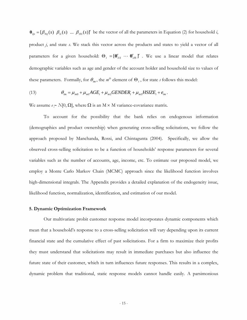
0 1 10[ ( ) ( ) ... ( )]ijs ij i is s s θ be the vector of all the parameters in Equation (2) for household i,

product j, and state s. We stack this vector across the products and states to yield a vector of all

parameters for a given household: i ] [ 11 iJSi θθ . We use a linear model that relates

demographic variables such as age and gender of the account holder and household size to values of

these parameters. Formally, for im , the mth element of i , for state s follows this model:

(13) 0 1 2 3im m m i m i m i imAGE GENDER HSIZE e .

We assume e i N[0, ], where is an M M variance-covariance matrix.

To account for the possibility that the bank relies on endogenous information

(demographics and product ownership) when generating cross-selling solicitations, we follow the

approach proposed by Manchanda, Rossi, and Chintagunta (2004). Specifically, we allow the

observed cross-selling solicitation to be a function of households’ response parameters for several

variables such as the number of accounts, age, income, etc. To estimate our proposed model, we

employ a Monte Carlo Markov Chain (MCMC) approach since the likelihood function involves

high-dimensional integrals. The Appendix provides a detailed explanation of the endogeneity issue,

likelihood function, normalization, identification, and estimation of our model.

5. Dynamic Optimization Framework

Our multivariate probit customer response model incorporates dynamic components which

mean that a household’s response to a cross-selling solicitation will vary depending upon its current

financial state and the cumulative effect of past solicitations. For a firm to maximize their profits

they must understand that solicitations may result in immediate purchases but also influence the

future state of their customer, which in turn influences future responses. This results in a complex,

dynamic problem that traditional, static response models cannot handle easily. A parsimonious

- 16 -

method that we propose to obtain the answer is to treat cross-selling decisions as solutions to a

stochastic dynamic optimization problem.

Specifically, we let the indicator value ijktZ designate cross-selling solicitations, where ijktZ

denotes the number of solicitations sent to household i for product j during period t using channel k

(k=1 for postal mail and k=2 for email):

(14) 1, if solicitation is sent to customer for product through channel at time 0, otherwise ijkt

i j k tZ

In other words, the manager makes the promotion or solicitation decision about when (t) to send

what product (j) to which customer (i) through which communication channel (k).

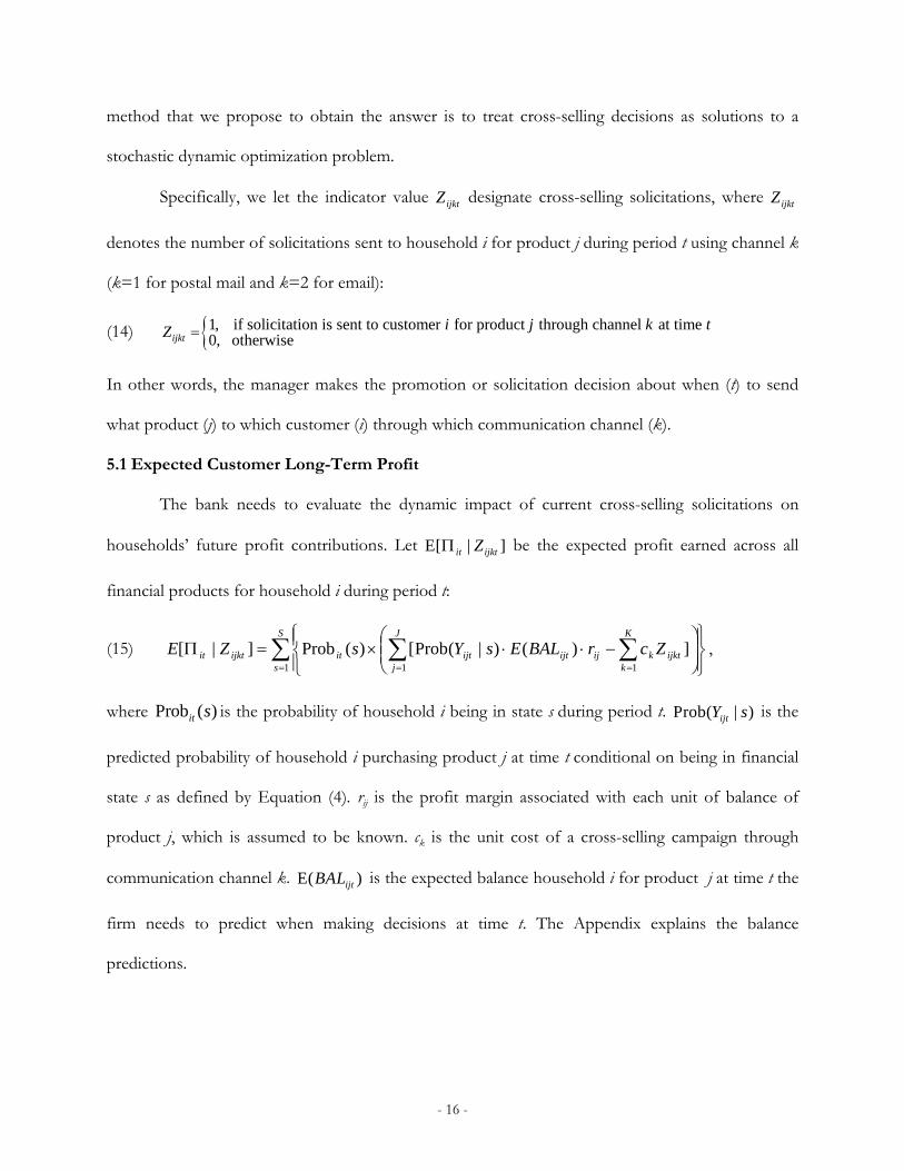
5.1 Expected Customer Long-Term Profit

The bank needs to evaluate the dynamic impact of current cross-selling solicitations on

households’ future profit contributions. Let E[ | ]it ijktZ be the expected profit earned across all

financial products for household i during period t:

(15)

S

s

J

j

K

kijktkijijtijtitijktit ZcrBALEsYsZE

1 1 1

])()|(Prob[)(Prob]|[ ,

where Prob ( )it s is the probability of household i being in state s during period t. Prob( | )ijtY s is the

predicted probability of household i purchasing product j at time t conditional on being in financial

state s as defined by Equation (4). rij is the profit margin associated with each unit of balance of

product j, which is assumed to be known. ck is the unit cost of a cross-selling campaign through

communication channel k. E( )ijtBAL is the expected balance household i for product j at time t the

firm needs to predict when making decisions at time t. The Appendix explains the balance

predictions.

- 17 -

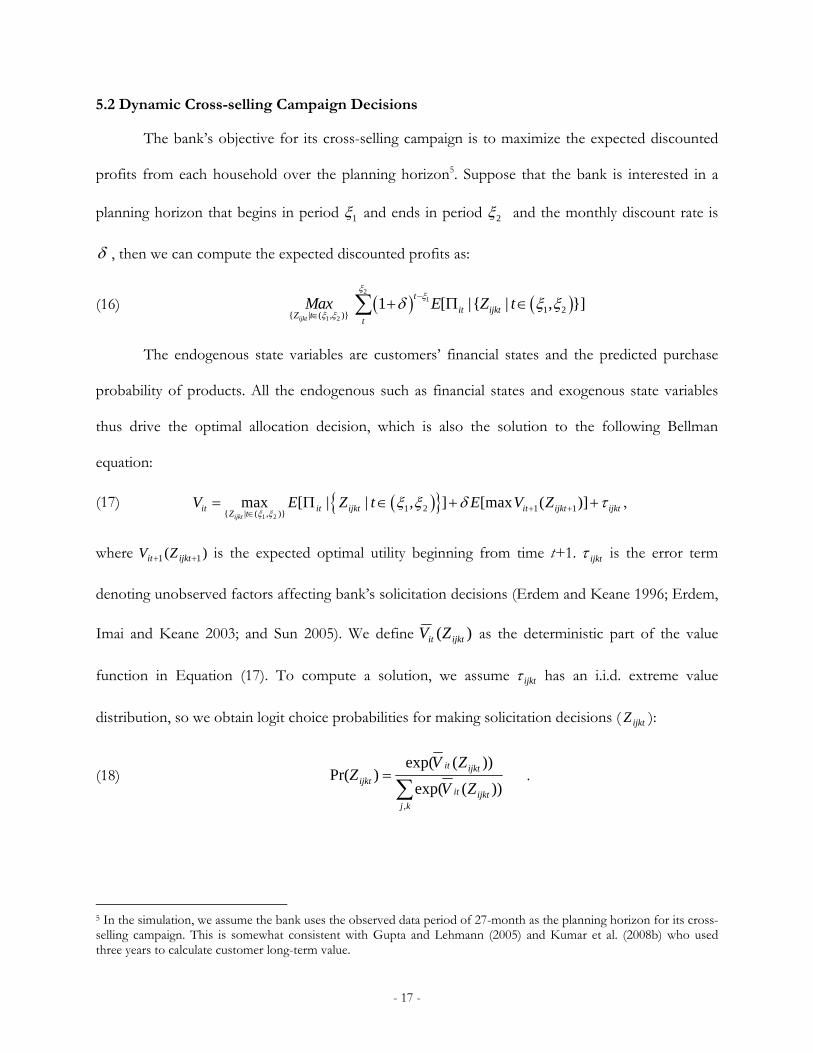
5.2 Dynamic Cross-selling Campaign Decisions

The bank’s objective for its cross-selling campaign is to maximize the expected discounted

profits from each household over the planning horizon5. Suppose that the bank is interested in a

planning horizon that begins in period 1 and ends in period 2 and the monthly discount rate is

, then we can compute the expected discounted profits as:

(16) 2

1

1 21 2

{ | ( , )}1 [ |{ | , }]

ijkt

t

it ijktZ t

t

Max E Z t

The endogenous state variables are customers’ financial states and the predicted purchase

probability of products. All the endogenous such as financial states and exogenous state variables

thus drive the optimal allocation decision, which is also the solution to the following Bellman

equation:

(17) 1 2

1 2 1 1{ | ( , )}

max [ | | , ] [max ( )]ijkt

it it ijkt it ijkt ijktZ t

V E Z t E V Z

,

where )( 11 ijktit ZV is the expected optimal utility beginning from time t+1. ijkt is the error term

denoting unobserved factors affecting bank’s solicitation decisions (Erdem and Keane 1996; Erdem,

Imai and Keane 2003; and Sun 2005). We define )( ijktit ZV as the deterministic part of the value

function in Equation (17). To compute a solution, we assume ijkt has an i.i.d. extreme value

distribution, so we obtain logit choice probabilities for making solicitation decisions ( ijktZ ):

(18)

kjijktit

ijktit

ijktZV

ZVZ

,

))(exp(

))(exp()Pr( .

5 In the simulation, we assume the bank uses the observed data period of 27-month as the planning horizon for its cross-selling campaign. This is somewhat consistent with Gupta and Lehmann (2005) and Kumar et al. (2008b) who used three years to calculate customer long-term value.

- 18 -

In order to overcome the challenge of large space, we adopt the interpolation method proposed by

Keane and Wolpin (1994) and approximate values for the expected maxima at any other state points

for which values are needed.

6. Empirical Results

6.1 Model Comparison

We compare our estimated customer response model against five benchmark models in

order to investigate the contribution of latent financial states, the long-term indirect roles

(educational and advertising) of cross-selling campaigns, and heterogeneous channel preferences to

predict customer purchase behavior. Model A is the latent financial maturity model proposed by Li,

Sun, and Wilcox (2005), which ignores the long-term roles of cross-selling and customer’s channel

preference, and assumes latent financial maturity is linearly determined by household account

ownership and experiences. Model B is the joint model of purchase timing and product category

choice by Kumar, Venkatesan, and Reinartz (2008a). In this model customer category purchase

choice is conditional upon purchase timing while ignoring the long-term roles of cross-selling. These

two benchmark models represent the most recent cross-selling models proposed in the marketing

literature. Model C is our proposed model without latent financial states, long-term effects of

solicitations, and heterogeneous preference for communication channels. Model D adds latent

financial states to the third model. However, we do not allow either long-term effects of solicitations

nor heterogeneous channel preferences. Model E adds long-term roles of advertising and education

to Model D, but not heterogeneous preferences for communication channels. Model F is our

proposed customer response model, which nests models C, D and E as special cases.

[Insert Table 3A and 3B about here]

To determine the number of states we estimate models with between one and four states,

and report the results in Table 3A. We find that the three-state version of the proposed model F is

- 19 -

the best-fitting model, subsequently we only report the three-state version for model F. Table 3B

reports the log of the marginal density (Chib and Greenberg 1995; Kass and Raferty 1995) and the

hit rates of product purchases for the six models. The overall hit-rate demonstrates how well our

model can predict future customer responses. To forecast future observations we calculate NACCT

at time t+1 as the sum of NACCT at t and the predicted new purchases at t, simulate the waiting

time from Equation 6, and condition upon other covariates. However, all models have access to the

same information to preserve comparability across the forecasts.

Since consumer purchase occur infrequently—roughly 3.1% of observations are purchases,

see the sum of purchase transactions as reported in Table 2—a naïve predictor of no purchase

would be correct 96.9% of the time. (Notice that all our models do better than this naïve prediction,

with performance between 97.3% and 99.5%.) To create a more challenging predictive task we

report the accuracy of these predictions for purchase and non-purchase observations separately6.

The comparison of model-fit and predictions across both the calibration sample and the two

validation samples shows our proposed model F significantly outperforms the benchmark models,

especially models A and B. These results suggest the innovations provided by our customer response

model are important.

6.2 Parameter Estimates

Tables 4A through 4E reports the estimation results of our proposed model F.

[Insert Table 4A-E about here.] 6 We predict purchase without knowledge about if purchase has occurred or not, and then report the hit rates separately for the purchase and non-purchase observations. For our multivariate choice model we must predict both when the purchase is going to occur as well as what is going to be purchased. This is different from multinomial choice model which only concerns itself with the latter. Hence, our overall hit-rate provides a measure of performance of incidence, while the hit-rates for the purchase and non-purchase samples measure accuracy of what is purchased. Consider the poorest performing Model A which has a hit-rate of 14.1% for the purchase sample, which is marginally worse than a naïve model which would predict purchase type correctly 14.3% of the time (the 14.3% can be found by the taking the average of the relative frequency of the type of product purchased from Table 2.) However, model A still has a superior overall hit rate of 98.5% which is substantially better than the naïve prediction of always guessing no purchase—which would only yield a 96.9% accuracy (i.e., 100% less the observed purchase frequency of 3.1%). Therefore a gain in accurately predicting when purchase occurs yields some tradeoff in accuracy of detecting what is going to be purchased.

- 20 -

Starting and Transition Probability Equation: First consider the parameters of the starting

probability and transition probability functions in Table 4A. We find that the probability that a

household starts in a higher financial state (Equation 12) increases with more accounts or more

assets deposited with the bank during the initial period, consistent with our intuition. Similarly, the

estimated hyper-parameters for such states with the transition probabilities (i.e. in Equation 11)

indicate that when a household switches states, it is more likely to switch to a higher state (i.e. state 2

or 3) than a lower ones (see the larger hyper-parameter estimates in higher states, p-value = .001 or 0

for state 2 and 3, respectively)7.

Waiting Time Equation: In the expected-waiting-time Equation (7), the constant terms in the

waiting-time function are estimated to be -8.23, -8.53, and 13.43 for the three states. The ordering of

the coefficients (negative constants in state 1 and 2) indicates that households have an intrinsic

preference to stay in state 3 for a longer time (p-values are .001). The coefficient of the number of

accounts in state 1 is negative and significant, implying that households with more financial products

are less likely to stay in states 1, while those with more are more likely to stay in states 2 or 3.

Comparing the product-specific coefficients on the number of solicitations, we find that

solicitations that promote checking, savings, others, and credit cards in the first state, those that

promote loans and CDs in the second state, and those that promote investment and loans in the

third state encourage customers to stay for a shorter period and to move faster along the financial-

state continuum (e.g., p-value = 0 for comparing investment coefficient with checking coefficient in

the third state). This supports our contention that offering the right product is important, since

checking account solicitations are helpful in shortening the customer’s time in the first state. This

7 The p-values reported in this section refer to the probability of a one-side test the differences between the coefficients are different than zero. They are computed based on the empirical probability of the difference being negative from our MCMC samples, which appropriately marginalizes across the uncertainty of the parameters. The small p-values are due to the fact that the data is well able to differentiate between the financial states and large number of observations provides strong information in making the inferences. However, the sampling error in our MCMC estimates mean the p-values have some chance of being higher than the 0 or .001 that is reported, but are clearly highly significant (<.01).

- 21 -

also illustrates that states are not solely determined by exogenous financial conditions (e.g.,

customer's age and income), but also marketing activity by the bank.

Comparing the coefficients of email and postal mail solicitations, we find that the

educational role is higher (more negative, p-values = .001 for all the three states) when the bank uses

email than when it uses postal mail possibly due to the rich information and interactive nature of

emails (Ansari and Mela 2003). However, the positive coefficients of the squared terms of these two

variables indicate that receiving too many solicitations reduce the effectiveness of the educational

role of campaigns, which agrees with findings in Venkatesan and Kumar (2004) and Venkatesan,

Kumar and Bohling (2007). This result is consistent with our conjecture that too many solicitations

wear out a customer’s attention, thereby reducing the marginal educational role.

Therefore, our results confirm the educational role of solicitations in helping households

move faster along the financial continuum when a bank solicits households on checking, savings,

others, and credit cards in the first state, loans and CDs in the second state, and investments and

loans in the third state. The educational role differs across communication channels and products. It

is more effective when a bank uses email than when it uses postal mail. However, the educational

role wears out when a bank sends too many solicitations to the same household. Interestingly, we

also find that the more accounts households close, the longer they stay in the first state and shorter

in the higher states (p-value = .001 or 0 for the second and third states respectively).

Purchase Equation: The estimates of the coefficients in the purchase utility model are given in

Table 4A, while the error correlation matrix is given in Table 4B. Based on the magnitude (from

high to low) of the estimated product-specific intercepts, we find that households in the first

financial state have an intrinsic preference for credit cards, checking and savings, followed by loans,

others, CDs, and investments. In the second state, the ranking is CDs and loan products, checking,

investment, others, savings, and credit cards. In the last state, the ranking is investment, checking,

- 22 -

credit cards, others, loans, savings, and CDs (e.g., p-value = 0 for comparing investment coefficient

with checking coefficient in the third state).

The coefficients of the solicitations in the current month measure the instantaneous effect of

promotions8. Comparing the product-specific solicitation effect, we show that the instantaneous

promotional effects are higher for checking, savings, credit cards and others in the first state, for

loans, CDs, checking and others in the second states, and for investment, checking and CDs in the

third state (e.g., p-value = 0 for comparing checking coefficient with saving coefficient in the first

state). The cumulative solicitations up to the current month also significantly increases the likelihood

the household will open new accounts. Households are likely to view receiving more solicitations as

a signal of customer care and relationship building and thus are encouraged to open new accounts

with this bank.

Both postal mail and email solicitations in the current month as well as solicitations for each

financial product increase the likelihood the household will open a new account for all three states.

Notice that both postal mail and email solicitations are slightly more effective in higher states (i.e.,

the second and third states, p-value = .001 or 0 when comparing the third state to the first state for

mail and email, respectively) because households in higher states may be more financially mature and

may have stronger relationships with the bank, thereby engendering trust and making them more

responsive to cross-selling solicitations (Kamakura, Ramaswami, and Srivastava 1991).

As expected, the positive coefficient on the mean change of financial assets increases the

probability of a household opening a new account with the bank. However, the variance of change

8 In our model, the coefficients of solicitations in the purchase utility model measure the responsiveness conditional on the household is in a particular state. The reason that our model results in more significant coefficients is that by taking into account intra-customer heterogeneity or evolvement of financial states, we recognize the situations when households are not ready for a particular financial product and thus not responsive to the cross-selling solicitations. However, this cannot be captured by models ignoring the evolvement of financial states. The same coefficient is estimated to be insignificant. Indeed, most parameters in Model C (the benchmark model ignoring indirect effects of solicitations) are not significant.

- 23 -

of total assets in the bank decreases the purchase probability. This result may be due to the fact that

the higher the mean of the balance change, the more assets are available, and a higher variance

means less financial stability (Li, Sun and Wilcox 2005). Interestingly, owning more accounts in

other product categories decreases the purchase probability of the focal category in the first state but

increases the purchase propensity in the second and third states. This may be due to the fact that

customers in low financial state may have financial resource constraints or low commitment to the

bank than those in higher states, which results in higher inter-category competition.

Customers with a higher number of cumulative transactions are more likely to open new

accounts with the bank due to the strengthening of the customer-seller relationship (Anderson and

Weitz 1992; Kalwani and Narayandas 1995). Tenure—measured by the length of time a household

has been a bank customer—increases the switching cost and hence the likelihood of opening new

accounts. A higher percentage of assets in other financial institutions decreases the probability of the

customer purchasing new accounts. Higher income increases the purchase propensity in all the three

states (Li, Sun and Wilcox 2005; Paas, Bijmolt and Vermunt 2007).

Interestingly, this ranking of the instantaneous solicitation effectiveness in the utility

function is roughly consistent with that of the educational effectiveness in the expected-waiting-time

equation. It is also quite similar to the ranking of the constant terms in the utility equation that

indicate household intrinsic preference. The results imply that households have different priorities

for various financial products during each financial state. In the first state, they demonstrate a higher

preference for checking, savings, and credit cards, or products that provide financial convenience,

and are more likely to respond to solicitations of these products. In the second state, they prefer and

are more likely to respond to solicitations selling loans and CDs, which reflect their need for

financial flexibility. In the third state, they prefer and are more likely to respond to solicitations

selling investment-related products. Based on the products customers are more likely to buy and

- 24 -

their responsiveness to the cross-selling campaigns in each state, we term the three states as a

convenience state, a flexibility state, and a growth state.

Household Heterogeneity: Table 4C reports the estimation results for the hierarchical component

of the utility equation. Most of the significantly estimated coefficients have the expected signs and

demonstrate that the instantaneous solicitation effect varies across households according to their

characteristics. Consider gender as an example. Notice that balance increases purchase probability

more for male customers, while tenure effects show that men are not as likely to remain loyal

perhaps because male customers are more likely to take advantage of competitive offers from other

financial institutions (Barber and Odean 2001). Male customers are also less likely to respond to

investment and loans solicitations perhaps because they believe themselves to be more

knowledgeable about the financial products and hence more confident in managing their

investments (Barber and Odean 2001)

Hidden Markov Process: Tables 4D and 4E present the estimation results for the HMM. Table

4D shows a household is most likely to start in a convenience state (first state) or in a growth state

(third state) with a 32 percent and 57 percent probability, respectively. We compute the average

waiting-times for each state to be 9.68, 10.90, and 15.07 for s =1, 2, and 3, respectively, based upon

Equation (7). Table 4E lists the transition probabilities for the HMM. Notice that households in our

study tend to have a higher probability of switching to convenience state (first state). For instance, if

a household is currently in the second state, the transition probability from the second to the first

state is 93 percent, while it is 7 percent for switching to the third state. Also, if a household is

currently in the third state, we estimate it has a 92 percent chance of switching from the third state

to the first state and an 8 percent probability of switching from the third state to the second state.9

9 Our proposed customer response model is general enough to allow the possibility for customers to move freely back and forth among states. A nested version of our proposed customer response model can constrain customers to move only up from state 1 to state 3. In our applications, the results show the general trend of consumers sequentially migrate

- 25 -

Consistent with our finding in the waiting time model, this may indicate the first state represents a

quiet attrition state in which households have low financial maturity and gradually close accounts.

6.3 Financial States

In this section, we investigate how and whether customers move along a financial continuum

over time. In Figure 1, we plot the average probabilities of customers residing in the three stages

against time. These probabilities are computed using a filtering approach to recover the individual’s

state at any given time period (Montgomery et al. 2004; Netzer, Lattin, and Srinivasan 2008). We

find customers tend to slowly move through time from the first state to the second state, and then

to the third state. In other words, customers begin in a financial state in which they are more likely

to look for convenience to a state in which they need financial flexibility and then to a state in which

they seek riskier growth investments.

[Insert Figure 1 and Table 5 about here]

6.4 Decomposition of Long-term Solicitation Effects

Given that cross-selling solicitations have demonstrated their instantaneous, advertising, and

educational roles, it is interesting to measure their relative strength. We arbitrarily pick a month

(month 3) during which little cross-selling solicitation occurs and choose loans as a cross-selling

solicitation example. We increase by 10 percent the frequency of households receiving loan

solicitations through postal mail and randomly select the recipients. Based on the posterior estimates

of the proposed customer response model, we report the probability changes of being in each of the

three financial states in columns 2-4 of Table 5. For example, an increase in loan solicitations during

month 3 results in a 0.90 percent increase in being in state 2, but a decrease of -0.44 percent and -

up from state 1 to state 2 to state 3, with some households are estimated to go back and forth (about 5.81% of the households). Reversion from more advanced states to earlier states may be due to consumer attrition, changes in their financial status, repeat purchases for other household members, or the aggregation of product variations.

- 26 -

0.46 percent of states 1 and 3, respectively. We also find that there is an instantaneous increase in

purchase probability of loans of 0.30 percent, which is listed in the column titled “Change of Prob

of Purchasing” in Table 5 (the numbers in the table are percentages).

The educational role of cross-selling occurs through the HMM process, specifically by

influencing the consumer’s switching to different financial states in the future. If we ignore the

probability of state changes and compute the effect of our increasing loan cross-selling then we can

estimate the direct effect of cross-selling promotions separately from the educational effect on the

purchase probability of loans. Our estimate of this direct effect of cross-selling on loan purchase

probability is given in Table 5 (“Direct Effect”). Initially in month 4 the increase in purchase

probability of loans is 0.14 percent, but by month 27 drops to 0.02 percent. Overall, this increases a

household’s cumulative purchase probability of loans by 1.88 percent from month 4 to month 27.

If we consider the state changes (e.g., which includes the educational role of cross-selling

through its influence on the state changes of the HMM) we find there is a much larger impact on

loan purchases from our hypothetical loan solicitation. Starting from the third month, we notice the

probabilities of households belonging to the second state (financial flexibility state) increase, whereas

those of the first state decrease (those of the third state first increase and then decrease). This means

the increase in loan solicitations in month 3 speeds up household movement along the financial

maturity continuum towards the flexibility state (state 2). Hence, over the course of months 3

through 27 we find a cumulative 12.72 percent increase in a consumer purchasing a loan. Among

this increase, only 2 percent (= .003/.127) is due to the instantaneous promotional effect, 15 percent

(= .019/.127) is due to the lasting advertising effect, and 83 percent (= (.127 - .003 - .019)/0.127)

comes from an educational effect. Thus, in this example the educational role of cross-selling

solicitations largely dominates the direct effects which include the instantaneous promotional and

advertising effects.

- 27 -

7. Simulating Customer-Centric Cross-Selling Solicitations

7.1 Dynamic and Customized Solicitations

[Insert Figure 2A and 2B about here]

On the basis of the estimated parameters, the observed history, and customer demographic

variables, we simulate optimal solicitation decisions ( *ijktZ ) using our proposed dynamic

programming framework (Equations 14 through 18). We obtain a sequence of cross-selling

campaign decisions ijktZ about when (t) to send out solicitations to which households (i) in order to

cross-sell which product (j) using which communication channel (k). To succinctly demonstrate how

the solicitations decisions are driven by financial states, in Figure 2A, we draw the average

probabilities of sending cross-selling campaigns on the J products *

1 1 1

1Pr( )

I K T

ijkti k t

ZI K T

against the three states. As shown in Figure 2A, our proposed cross-selling campaigns are developed

according a customer’s financial maturity state. For example, the probability of sending out

convenience-related financial products (such as checking and saving accounts) is highest in the first

state, and the probability of sending out more complex products, such as loans and CD’s in the

second state and investments in the third state is the highest.

Based on the findings from Figures 1 and 2A, during earlier observation periods that

correspond to the earlier financial stages of an average customer in our sample, we recommend

solicitations for checking and savings. During the middle observation period, our proposed solution

suggests sending this customer promotions that concern CDs and lending-related financial products.

During the latter part of our observation period, the solution recommends sending out investment-

related products. Thus, our proposed solution is dynamic in that the decisions of when and which

products to send solicitations are made in accordance with the household’s evolving financial

maturity state.

- 28 -

We next use age as an example to show how the proposed solicitations are customized

according to customer heterogeneity and channel preference (whom to send the solicitations and

using which channel). In Figure 2B, we again take loans as an example and plot the probability of

sending a solicitation, given by

T

tijktZ

T 1

* )Pr(1

, for this product against age. In order to demonstrate

whether the customization differs across communication channels, we draw the curve for both email

and postal mail channels. This snap-shot analysis allows us to show how the proposed solution is

tailored to age. We show that the probabilities of sending out loan solicitations using mails to

middle-aged customers (age 30-45) are higher than for other customers. This finding is consistent

with our intuition that middle-aged customers are more likely to be raising families and need to

borrow money to buy a house or pay for their children’s education. Note that the solution suggests

the solicitation channel should be customized for demographics and channel preference: they should

be sent through email for younger customers and through postal mail for older customers.

7.2 Improvement of Long-term Response Rates and Profit over Alternative Frameworks

Finally, we compare the response rates of our proposed solicitation solutions with a few

alternative approaches against those observed in our sample. In the first alternative framework, we

follow conventional industry practices as observed in our dataset and compute the sample product

ownership transition matrix (e.g., the purchase probabilities conditional on owning a particular

product). This sample transition matrix approach simply makes use of the observed purchase

ordering (i.e., first-order product transition matrix) from the estimation sample to predict customers’

purchases. For brevity we refer to this as the campaign-centric approach.

In the second alternative framework, we estimate a logit model that is similar to existing

cross-selling customer response models such as Li, Sun and Wilcox (2005). This approach assumes

the latent financial maturity is linearly determined by household account ownership and experiences.

- 29 -

Logit models were used to predict the response rate. Those customers with the highest expected

profit are offered the campaign. Thus, the solicitation decisions are made in a myopic way.

The third alternative framework is similar to Kumar et al. (2008a) by targeting customers

with the higher long-term value. Customer long-term value is calculated as the net present value of

the predicted stream of future profits. This framework does not account for intra-customer

heterogeneity, nor does the bank employ dynamic programming to optimize future actions.

The fourth alternative approach follows a customer response model that ignores financial

maturity, intra-customer heterogeneity and long-term effects of solicitations (Model C). The

optimization framework is myopic and ignores customer life time value.

The fifth and sixth alternative approaches allow the customer response model to take into

account both intra-customer heterogeneity and long-term effects of solicitations (Model F). The

fifth framework assumes the bank is myopic, while the sixth framework incorporates customer life

time value and follows our proposed dynamic optimization framework.

[Insert Table 6 about here]

In Table 6, we report and compare the number of mail and email solicitations sent out, the

short-term and long-term response rates, total profit, and return on investment (ROI) during our

observation period using the calibration sample10. Notice that our proposed framework does not

result in the highest short-term response rate. Instead, our objective is to maximize the long-term

response rate—which we find to be significantly higher than all the other techniques. Our gains

occur by recognizing the financial readiness of a customer and long-term effects of solicitation on

customer responses. The result is a sequence of solicitation decisions that maximize long-term

customer (response rate) and profit. This means some solicitations are not sent to seek an immediate

response, but to help educate customers and prepare them for future solicitations. Additionally,

10 We obtain similar results using the cross-sectional holdout sample. The improvement of ROI is 53.4 percent.

- 30 -

notice that the total number of mail solicitations resulting from our dynamic optimization

framework is about half of current practices as observed in the data. Hence, recognizing the

customer’s financial development reduces irrelevant messages.

Comparing the 5.1 percent response rate from cross-selling solicitations of the campaign-

centric approach, the long-term response rate based on the proposed framework (Alternative 6) is

12.7 percent–a significant 149 percent (131 percent) improvement. ROI improves by 78.1 percent

and the total profit improves by 177 percent. Similar comparison holds for the first alternative

framework.

Both the immediate response rates and long-term response rates resulting from Li, Sun and

Wilcox (2005) and Kumar et al. (2008a) are improved over those observed in the sample and the

first alternative. These two approaches improve over the first alternative approach because customer

lifetime value (CLV) is treated as another segmentation variable to differentiate profitable customers

from unprofitable ones. However, the improvement of long-term response rate, total profit and

ROI are not as impressive as our proposed approach. This is because both frameworks ignore intra-

customer heterogeneity and long-term effects of solicitations and treating CLV as another

segmentation variable is different from our proposed dynamic programming approach.

Based on individual customer response model, the fourth alternative improves over the

campaign-centric approach because it allows for individual targeting. As expected, the fifth

alternative framework results in higher short-term and long-term response rates than those observed

in the sample. This is because it allows the bank to follow the evolution of each household and

makes a customized and dynamic solicitation schedule for each household. However, being myopic,

this framework cannot be proactive in taking advantage of the long-term educational role. Thus, it

results in lower long-term response rate compared to the proposed framework.

- 31 -

Our proposed framework (the sixth alternative) takes into account the development of

customers, the educational role of solicitations in impacting future response, and seeking to

maximize long-term profit. The improvement of performance dominates all the other alternative

decision frameworks. Comparing the magnitudes of improvements of Alternatives 4 to 6, we find

that improvement in long-term response rate and total profit are highest when dynamic decisions are

made, followed by proactive decision making and customization, respectively. The improvement on

ROI is highest when decisions are made in a proactive decision making, followed by dynamic

decisions and customization, respectively.

8. Conclusions, Limitations, and Future Research Directions

Low response rates are challenging managers to improve the effectiveness of cross-selling

campaigns. We believe current cross-selling focuses too much on individual campaigns and not

enough on the dynamic effects inherent in a customer-centric approach. We find that cross-selling

campaigns can be improved by understanding how cross-selling solicitations change customer

purchase behavior and tailoring these campaigns to each customer’s evolving needs and preferences

in order to enhance long-term customer relationships and optimize long-term profits.

Using cross-selling campaigns and purchase history data provided by a national bank, we

propose and estimate a customer-response model that recognizes latent financial maturity and

preference for communication channels. Our framework allows cross-selling solicitations to

influence the customer’s latent financial state so that they may become more receptive to particular

products in the future. Our results demonstrate that customer responses to cross-selling solicitations

of different products do indeed evolve over time. In addition, cross-selling solicitations help

customers by moving them in the future to a latent state when the customer prefers the cross-sold

product (educational role) or building up a long-term relationship (advertising role). Decomposition

of the instantaneous promotional, educational, and advertising effects of cross-selling in our study

- 32 -

reveals that the educational effect dominates the instantaneous promotional and advertising effects.

Furthermore, we find that relative to postal mail solicitations, email solicitations are more effective at

more advanced stages of customer financial maturity and are more effective at educating customers.

We show that the bank’s decisions should be part of an integrated multi-step, multi-segment,

and multi-channel cross-selling campaign process and show that the long-term response rate and

profit of a cross-selling campaign are significantly improved over existing myopic approaches. Ours

is the first study to explicitly investigate how cross-selling solicitations dynamically interact with

customer purchase decisions in the short and long runs. It also establishes the importance for the

bank to take a long-term view and develop a proactive sequence of campaign massages to influence

the growth path of households’ financial maturity.

Our dynamic programming approach serves as analytical decision-making tool for analyzing

rich customer databases and deriving concrete solutions on how to target the right customer with

the right product at the right time with the right channel. It also provides a computational algorithm

for firms that are looking for one-on-one, interactive, and real-time marketing solutions enabled by

current technology. Potentially simplified heuristics could approximate our decision rule. For

example, the current practice of cross-selling financial products to customers based on a snap shot

of their current demographics and product ownership approximates the customization property.

However, this simplified heuristic does not well approximate the dynamic and proactive elements of

our strategy and leaves room for improvement by incorporating dynamic and proactive properties.

This research is subject to limitations and opens avenues for future research. First, our study

is limited by a two-year history and lack of competition information. A sample with longer

longitudinal data and more complete information on competitors’ offers would expose the model to

changing competitive conditions, economic cycles and interest rates, and more longitudinal variation

in customer history. Second, many banks emphasize account acquisition and overlook retention of

- 33 -

account balances. Future research could explicitly model of account closings as well as account

openings. A third direction for future research is to study the migration of service channels (Ansari,

Mela, and Neslin 2008). Fourth, future researchers need to show how solicitations increase customer

financial knowledge and explicitly test the educational role of solicitation. Finally, future research can

take into account the effect of solicitations on usage, account balance, and customer retention,

which is beyond the scope of our research

References Aaker, Jennifer, Susan Fournier, and Adam S. Brasel. 2004. When good brands do bad. Journal of

Consumer Research 31 (June): 1-18. Allenby, Greg M., and Peter E. Rossi. 1999. Marketing Models of Consumer Heterogeneity. Journal

of Econometrics 89: 57-78. Anderson, Erin and Bart Weitz (1992), The Use of Pledges to Build and Sustain Commitment in

Distribution Channels. Journal of Marketing Research, 24 (February), 18-34. Ansari, Asim, and Carl F. Mela. 2003. E-Customization. Journal of Marketing Research 40 (2): 131-45. --------, Carl F. Mela, and Scott A. Neslin. 2008. Customer Channel Migration. Journal of Marketing

Research 45 (1) (February): 60-76. Authers, John. 1998. Cross-Selling’s Elusive Charms. Financial Times Nov 16: 21. Barber B., and T. Odean. 2001. Boys will be Boys: Gender, Overconfidence, and Common Stock

Investment. Quarterly Journal of Economics 116 (1): 261-92. Berger, Paul D., and Nada I. Nasr. 1998. Customer Lifetime Value: Marketing Models and

Applications. Journal of Interactive Marketing 12 (Winter): 17-30. Business Wire. 2000. 98% Market Failure Rate Now Obsolete for Financial Institutions. Business

Wire Nov. 15. Chib, Siddhartha and Edward Greenberg (1995). Understanding the Metropolis Hastings Algorithm.

American Statistician, 49, 327-335. Du, Rex, and Wagner Kamakura. 2006. Household Life Cycles and Lifestyles in the United States.

Journal of Marketing Research 43 (1): 121-32. Dwyer, Robert F. 1989. Customer Lifetime Valuation to Support Marketing Decision Making.

Journal of Interactive Marketing. 3(4): 8-15. --------, Paul H. Schurr, and Sejo Oh. 1987. Developing Buyer-Seller Relationships. Journal of

Marketing 51 (Apr.): 11-27. Erdem, Tulin and Michael P. Keane. 1996. Decision-making under uncertainty: Capturing dynamic

brand choice processes in turbulent consumer goods markets. Marketing Science. 15(1): 1-20. --------, S. Imai, and Michael P. Keane. 2003. Brand and Quantity Choice Dynamics under Price

Uncertainty. Quantitative Marketing and Economics. 1(1): 5-64. Edwards, Yancy D., and Greg M. Allenby. 2003. Multivariate Analysis of Multiple Response Data.’

Journal of Marketing Research. 40(3): 321-334. Fader, Peter S., Bruce G.S. Hardie, and Ka Kok Lee. 2005. Counting Your Customers’ the Easy

Way: An Alternative to the Pareto/NBD Model. Marketing Science, 24: 275-284. Fournier, Susan. 1998. Consumers and Their Brands: Developing Relationship Theory in Consumer

Research. Journal of Consumer Research 24 (Mar.): 343-73.

- 34 -

Gelfand, A E., and A.F. M. Smith. 1990. Sampling-Based Approaches to Calculating Marginal Densities. Journal of the American Statistical Association 85: (410): 398-409.

Gupta, Sunil, Donald R. Lehmann, and Jennifer A. Stuart. 2004. Valuing Customers. Journal of Marketing Research. (February): 7-18.

-------- and Donald R. Lehmann. 2006. Customer Lifetime Value and Firm Valuation. Journal of Relationship Marketing. 5 (2/3).

Heckman, James J. 1981. The Incidental Parameters Problem and The Problem of Initial Conditions in Estimating a Discrete Time-Discrete Data Stochastic Process. In Structural Analysis of Discrete Data with Econometric Applications, edited by C. F. Manski and D. McFadden. Cambridge: MIT Press: 179-95.

Jackson, D. R. 1996. Achieving Strategic Competitive Advantage Through the Application of The Long-term Customer Value concept, Journal of Database Marketing, 4(2): 174-186.

Kalwani, Manohar and Narakesari Narayandas (1995), “Long-Term Manufacturer-Supplier Relationships: Do They Pay Off for Supplier Firms?” Journal of Marketing, 59 (January), 1-16.

Kamakura W., S. Ramaswami, and R. Srivastava. 1991. Applying Latent Trait Analysis in the Evaluation of Prospects for Cross-Selling of Financial Services. International Journal of Research in Marketing 8: 329-49.

--------, Bruce S. Kossar, Michel Wedel. 2004. Identifying Innovators for the Cross-Selling of New Products. Management Science, 50(8): 1120-1133.

--------, A. M. Wedel, F. de Rosa, and J. A. Mazzon. 2003. Cross-Selling through Database Marketing: A Mixed Data Factor Analyzer for Data Augmentation and Prediction. International Journal of Marketing Research. 20(1): 45-65.

Kass, R., and A. Raferty. 1995. Bayes Factors. Journal of the American Statistical Association 90 (430): 773-95.

Keane, Michael P, Kenneth I. Wolpin. 1994. The Solution and Estimation of Discrete Choice Dynamic Programming Models by Simulation and Interpolation: Monte Carlo Evidence, The Review of Economics and Statistics, 76(4): 648-72.

Knott Aaron, Andrew Hayes, and Scott A. Neslin. 2002. Next-Product-to-Buy Models for Cross-Selling Applications. Journal of Interactive Marketing, 16(3): 59-75.

Krishna, Aradhna, Imran S. Currim, and Robert W. Showmaker. 1991. Consumer Perceptions of Promotional Activity. Journal of Marketing 55(2): 4-17.

Kumar, V., Rajkumar Venkatesan and Werner Reinartz (2008a), “Performance Implications of Adopting A Customer-Focused Sales Campaign,” Journal of Marketing, 72 (September), 50-68.

--------, Rajkumar Venkatesan, Tim Bohling and Denise Beckman (2008b), “The Power of CLV: Managing Customer Lifetime Value at IBM,” Marketing Science, 27 (4), 585-599.

Lewis, Michael. 2005a. A Dynamic Programming Approach to Customer Relationship Pricing. Management Science 51 (6): 986-994.

--------. 2005b. Incorporating Strategic Consumer Behavior into Customer Valuation. Journal of Marketing 69 (3), 230-238.

Li, Shibo, John C. Liechty, and Alan L. Montgomery. 2005. Modeling Category Viewership of Web Users with Multivariate Count Models.

[http://www.andrew.cmu.edu/~alm3/papers/web%20category%20viewership.pdf] --------, Baohong Sun, and Ronald T. Wilcox (2005), "Cross-Selling Sequentially Ordered Products:

An Application to Consumer Banking Services," Journal of Marketing Research, XLII, May, 233-239. Liechty, John C., Michel Wedel, and Rik Pieters. 2003. The Representation of Local and Global

Scanpaths in Eye Movements Through Bayesian Hidden Markov Models. Psychometrika 68 (4): 519-42.

- 35 -

Little, John D. C. 1979. Aggregate Advertising Models: The State of the Art. Operations Research 27 (Jul.-Aug.): 629–67.

Lodish, Leonard M., Magid Abraham, S. Kalmenson, J. Livelsberger, Beth Lubetkin, B. Richardson, and M. E. Stevens. 1995. How TV Advertising Works: A Meta-Analysis of 389 Real World Split Cable TV Advertising Experiments, Journal of Marketing Research 32 (1): 125–39.

Manchanda, Puneet, Asim Ansari, and Sunil Gupta. 1999. The "Shopping Basket": A Model for Multi-category Purchase Incidence Decisions. Marketing Science 18: 95-114.

--------, Peter E. Rossi and Pradeep K. Chintagunta 2004. Response Modeling with Nonrandom Marketing-Mix Variables. Journal of Marketing Research 41 (4): 467-478

Mehta, Nitin, Xinlei (Jack) Chen and Om Narasimhan, 2008. Informing, Transforming, and Persuading: Disentangling the Multiple Effects of Advertising on Brand Choice Decisions. Marketing Science 27 (3): 334-355.

Montgomery, Alan L., Shibo Li, Kannan Srinivasan, and John C. Liechty. 2004. Modeling Online Browsing and Path Analysis Using Clickstream Data. Marketing Science 23 (4): 579-95.

Moon, Sangkil, Wagner A. Kamakura, and Johannes Ledolter. 2007. Estimating Promotion Response When Competitive Promotions Are Unobservable. Journal of Marketing Research 44 (3): 503-15.

Mulhern, F.J. 1999. "Customer Profitability Analysis: Measurement, Concentra-tion, and Research Directions." Journal of Interactive Marketing 13 (1): 25-40.

Narayanan, S. and P. Manchanda, 2009. Heterogeneous Learning and the Targeting of Marketing Communication for New Products. Marketing Science 28(3):424-441.

Netzer, Oded, James. M. Lattin, and V. Srinivasan. 2008. A Hidden Markov Model of Customer Relationship Dynamics. Marketing Science 27(2): 185 – 204.

Paas, Leonard J., Tammo H.A. Bijmolt, and Jeroen K.Vermunt. 2007. Acquisition Patterns of Financial Products: A Longitudinal Investigation. Journal of Economic Psychology 28: 229-41.

Reinartz, Werner J., and V. Kumar. 2003. The Impact of Customer Relationship Characteristics on Profitable Lifetime Duration. Journal of Marketing. 67(January): 77-99.

--------, Jacquelyn S. Thomas and V. Kumar (2005), “Balancing Acquisition and Retention Resources to Maximize Customer Profitability,” Journal of Marketing, 69 (January), 63-79.

Rough Notes 2010. Beyond Cross-Selling. Rough Notes March 22, 2010. http://insurancenewsnet.com/article.aspx?id=173758.

Rosen, Theodore A. 2004. Why Your Bank Will Fail at Cross-Selling. Commercial Lending Review 19(2): 41-44.

Rust, Roland T., and Tuck Siong Chung. 2006. Marketing Models of Service and Relationships. Marketing Science. 25(6): 560-580.

--------, Katherine N. Lemon, and Valarie A. Zeithaml. 2004. Return on Marketing: Using Customer Equity to Focus Marketing Strategy. Journal of Marketing 68 (1): 109-27.

--------, and Peter Verhoef, 2005. Optimizing the Marketing Interventions Mix in Intermediate-Term CRM, Marketing Science, 24(3), 477-489.

Smith, Brad. 2006. The Future of Cross-Selling. Canadian Underwriter 73 (9) (Sept.): 32-33. Sun, Baohong, Shibo Li, and Catherine Zhou (2006), “‘Adaptive’ Learning and ‘Proactive’

Customer Relationship Management”, Journal of Interactive Marketing, Vol. 20, No. 3-4, 82-96. --------. 2005. Promotion Effect on Endogenous Consumption. Marketing Science. 24(3): 430-443. Venkatesan, Rajkumar and V. Kumar (2004), “A Customer Lifetime Value Framework for Customer

Selection and Resource Allocation Strategy,” Journal of Marketing, 68 (October), 106-125. --------, Rajkumar, V. Kumar and Timothy Bohling (2007), “Optimal Customer Relationship

Management Using Bayesian Decision Theory: An Application for Customer Selection,” Journal of Marketing Research, XLIV (November), 579-594.

- 36 -

Table 1. Summary of Literature on Cross-Selling and Customer-Lifetime Value Analysis

Paper

Product Owner -ship

Measuring Effectiveness

of Cross-Selling

Long- Term Role of Cross-Selling

Intra-Customer Hetero-geneity CLV

Dynamic Program-

ming Edwards & Allenby 2003 Kamakura et al. 2003 Knott, Hayes & Neslin 2002 Kamakura, Ramaswami, &

Srivastava 1991 Li, Sun & Wilcox 2005

Berger & Nasr 1998 Dwyer 1989 Fader, Hardie & Lee 2005 Jackson 1996 Mulhern 1999 Rust, Lemon & Zeithaml

2004

Lewis 2005a,b Rust & Chung 2006

Reinartz, Thomas & Kumar 2005

Rust & Verhoef 2005 Venkatesan and Kumar

2004 Kumar et al. 2008a Venkatesan, Kumar &

Bohling 2007

Du & Kamakura 2006 Netzer, Lattin & Srinivasan

2008

Our study

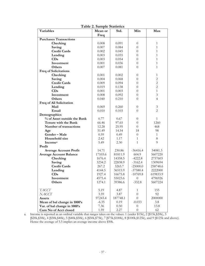
- 37 -

Table 2. Sample Statistics Variables

Mean or Freq

Std. Min Max

Purchases Transactions Checking Saving Credit Cards Lending CDs Investment Others

Freq of Solicitations Checking Saving Credit Cards Lending CDs Investment Others

Freq of All Solicitation Mail Email

Demographics % of Asset outside the Bank Tenure with the Bank Number of transactions Age Gender – Male Household size Incomea Profit Average Account Profit Average Account Balance

Checking Saving Credit Cards Lending CDs Investment Others

TACCT NACCT Assets Mean of bal change in 1000’s Var. of bal change in 1000’s Cum No of Acct closed

0.008 0.007 0.002 0.003 0.003 0.001 0.007

0.001 0.004 0.009 0.019 0.001 0.008 0.040

0.069 0.010

0.77 66.46 12.28 51.49 0.59 2.42 5.49

14.71

17103.6 1676.4 3234.2 267.2 4144.5 1927.4 4575.4 1274.1

5.19 3.59

97243.4 -6.35 7.36 1.59

0.091 0.084 0.045 0.055 0.054 0.036 0.081

0.002 0.068 0.094 0.138 0.003 0.092 0.210

0.260 0.103

0.67 97.65 25.95 14.54 0.49 1.17 2.30

230.86 81811.9 14358.5 22838.9 3265.7 36515.9 16675.8 55023.6 39386.6

4.87 3.87

187748.1 0.19 0.50 2.27

0 0 0 0 0 0 0 0 0 0 0 0 0 0 0 0 0 0 0 18 0 1 1

-36416.4 604.9

-4222.8 -3162.4 -25000.0 -37580.4 -10769.8

0 -332.8

1 0 0

-0.033 0 0

1 1 1 1 1 1 1 1 2 2 2 1 3 4 3 2 1

1260 468 98 1 8 9

34081.3 5607220 2757603 1309694 258748.6 2222000 619833.9 4796926 5607224

155 92

2000000 3.8 13.8 62

a. Income is reported as an ordinal variable that ranges takes on the values: 1 (under $15k), 2 [$15k,$20k), 3 [$20k,$30k), 4 [$30k,$40k), 5 [$40k,$50k), 6 [$50k,$75k), 7 [$75k,$100k), 8 [$100k,$125k), and 9 [$125k and above). Hence the average of 5.5 implies an average income above $50k.

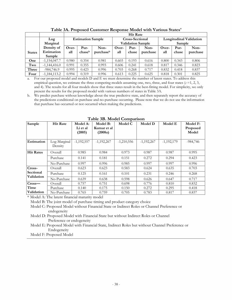
- 38 -

Table 3A. Proposed Customer Response Model with Various Statesa Hit Rate

States

Log Marginal

Density of Estimation

Sample

Estimation Sample Cross-Sectional Validation Sample

Longitudinal Validation Sample

Over- all

Pur-chaseb

Non-purchaseb

Over-all

Pur-chase

Non-purchase

Over-all

Pur-chase

Non-purchase

One -1,154,047.7 0.980 0.354 0.981 0.603 0.193 0.616 0.800 0.343 0.806Two -1,144,416.0 0.991 0.355 0.993 0.606 0.241 0.618 0.817 0.346 0.823

Three -984,746.9 0.995 0.423 0.996 0.703 0.268 0.717 0.832 0.418 0.837Four -1,184,113.2 0.994 0.319 0.996 0.613 0.225 0.625 0.818 0.301 0.825

a. For our proposed model and models D and E we must determine the number of latent states. To address this empirical question, we estimate the three competing models assuming one, two, three, and four states (s =1, 2, 3, and 4). The results for all four models show that three states result in the best-fitting model. For simplicity, we only present the results for the proposed model with various numbers of states in Table 3A.

b. We predict purchase without knowledge about the true predictive state, and then separately report the accuracy of the predictions conditional on purchase and no-purchase occurring. Please note that we do not use the information that purchase has occurred or not occurred when making the predictions.

Table 3B. Model Comparison Sample Hit Rate Model A:

Li et al (2005)

Model B: Kumar et al

(2008a)

Model C

Model D

Model E

Model F:Proposed

Model

Estimation

Log-Marginal Density

-1,192,557 -1,192,267 -1,210,556 -1,192,267 -1,192,179 -984,746

Hit Rates Overall 0.985 0.984 0.973 0.987 0.987 0.995

Purchase 0.141 0.181 0.151 0.272 0.294 0.423

No-Purchase 0.997 0.996 0.985 0.997 0.997 0.996Cross-Sectional Validation

Overall 0.623 0.623 0.583 0.624 0.635 0.703

Purchase 0.125 0.161 0.101 0.231 0.246 0.268

No-Purchase 0.639 0.638 0.598 0.626 0.647 0.717Cross— Time Validation

Overall 0.757 0.751 0.698 0.776 0.810 0.832Purchase 0.140 0.175 0.150 0.272 0.295 0.418No-Purchase 0.765 0.759 0.705 0.783 0.817 0.837

* Model A: The latent financial maturity model Model B: The joint model of purchase timing and product category choice Model C: Proposed Model without Financial State or Indirect Roles or Channel Preference or endogeneity Model D: Proposed Model with Financial State but without Indirect Roles or Channel Preference or endogeneity Model E: Proposed Model with Financial State, Indirect Roles but without Channel Preference or Endogeneity Model F: Proposed Model

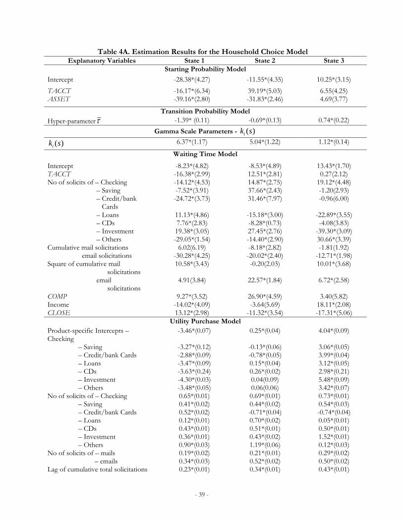
- 39 -

Table 4A. Estimation Results for the Household Choice Model Explanatory Variables State 1 State 2 State 3

Starting Probability Model

Intercept -28.38*(4.27) -11.55*(4.35) 10.25*(3.15)

TACCT -16.17*(6.34) 39.19*(5.03) 6.55(4.25) ASSET -39.16*(2.80) -31.83*(2.46) 4.69(3.77)

Transition Probability Model Hyper-parameter -1.39* (0.11) -0.69*(0.13) 0.74*(0.22)

Gamma Scale Parameters - ( )ik s

( )ik s 6.37*(1.17) 5.04*(1.22) 1.12*(0.14)

Waiting Time Model

Intercept -8.23*(4.82) -8.53*(4.89) 13.43*(1.70) TACCT -16.38*(2.99) 12.51*(2.81) 0.27(2.12) No of solicits of – Checking -14.12*(4.53) 14.87*(2.75) 19.12*(4.48) – Saving -7.52*(3.91) 37.66*(2.43) -1.20(2.93) – Credit/bank Cards

-24.72*(3.73) 31.46*(7.97) -0.96(6.00)

– Loans 11.13*(4.86) -15.18*(3.00) -22.89*(3.55) – CDs 7.76*(2.83) -8.28*(0.73) -4.08(3.83) – Investment 19.38*(3.05) 27.45*(2.76) -39.30*(3.09) – Others -29.05*(1.54) -14.40*(2.90) 30.66*(3.39) Cumulative mail solicitations 6.02(6.19) -8.18*(2.82) -1.81(1.92) email solicitations -30.28*(4.25) -20.02*(2.40) -12.71*(1.98) Square of cumulative mail solicitations

10.58*(3.43) -0.20(2.03) 10.01*(3.68)

email solicitations

4.91(3.84) 22.57*(1.84) 6.72*(2.58)

COMP 9.27*(3.52) 26.90*(4.59) 3.40(5.82) Income -14.02*(4.09) -3.64(5.69) 18.11*(2.08) CLOSE 13.12*(2.98) -11.32*(3.54) -17.31*(5.06)

Utility Purchase Model Product-specific Intercepts – Checking

-3.46*(0.07) 0.25*(0.04) 4.04*(0.09)

– Saving -3.27*(0.12) -0.13*(0.06) 3.06*(0.05) – Credit/bank Cards -2.88*(0.09) -0.78*(0.05) 3.99*(0.04) – Loans -3.47*(0.09) 0.15*(0.04) 3.12*(0.05) – CDs -3.63*(0.24) 0.26*(0.02) 2.98*(0.21) – Investment -4.30*(0.03) 0.04(0.09) 5.48*(0.09) – Others -3.48*(0.05) 0.06(0.06) 3.42*(0.07) No of solicits of – Checking 0.65*(0.01) 0.69*(0.01) 0.73*(0.01) – Saving 0.41*(0.02) 0.44*(0.02) 0.54*(0.03) – Credit/bank Cards 0.52*(0.02) -0.71*(0.04) -0.74*(0.04) – Loans 0.12*(0.01) 0.70*(0.02) 0.05*(0.01) – CDs 0.43*(0.01) 0.51*(0.01) 0.50*(0.01) – Investment 0.36*(0.01) 0.43*(0.02) 1.52*(0.01) – Others 0.90*(0.03) 1.19*(0.06) 0.12*(0.03) No of solicits of – mails 0.19*(0.02) 0.21*(0.01) 0.29*(0.02) – emails 0.34*(0.03) 0.52*(0.02) 0.50*(0.02) Lag of cumulative total solicitations 0.23*(0.01) 0.34*(0.01) 0.43*(0.01)

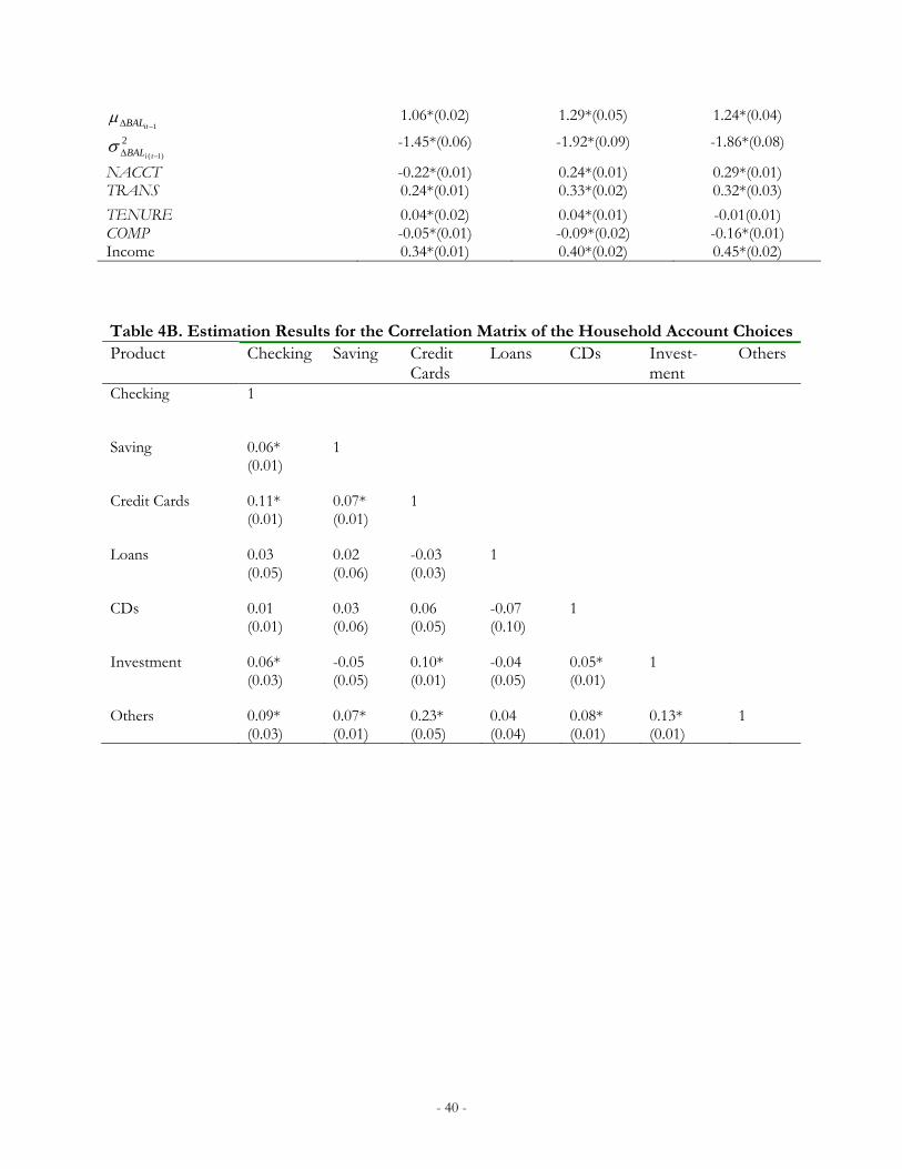
- 40 -

1 itBAL 1.06*(0.02) 1.29*(0.05) 1.24*(0.04)

2

)1( tiBAL -1.45*(0.06) -1.92*(0.09) -1.86*(0.08)

NACCT -0.22*(0.01) 0.24*(0.01) 0.29*(0.01) TRANS 0.24*(0.01) 0.33*(0.02) 0.32*(0.03)

TENURE 0.04*(0.02) 0.04*(0.01) -0.01(0.01) COMP -0.05*(0.01) -0.09*(0.02) -0.16*(0.01) Income 0.34*(0.01) 0.40*(0.02) 0.45*(0.02)

Table 4B. Estimation Results for the Correlation Matrix of the Household Account Choices Product Checking Saving Credit

Cards Loans CDs Invest-

ment Others

Checking 1

Saving 0.06*

(0.01) 1

Credit Cards 0.11*

(0.01) 0.07* (0.01)

1

Loans 0.03

(0.05) 0.02 (0.06)

-0.03 (0.03)

1

CDs 0.01

(0.01) 0.03 (0.06)

0.06 (0.05)

-0.07 (0.10)

1

Investment 0.06*

(0.03) -0.05 (0.05)

0.10* (0.01)

-0.04 (0.05)

0.05* (0.01)

1

Others 0.09*

(0.03) 0.07* (0.01)

0.23* (0.05)

0.04 (0.04)

0.08* (0.01)

0.13* (0.01)

1

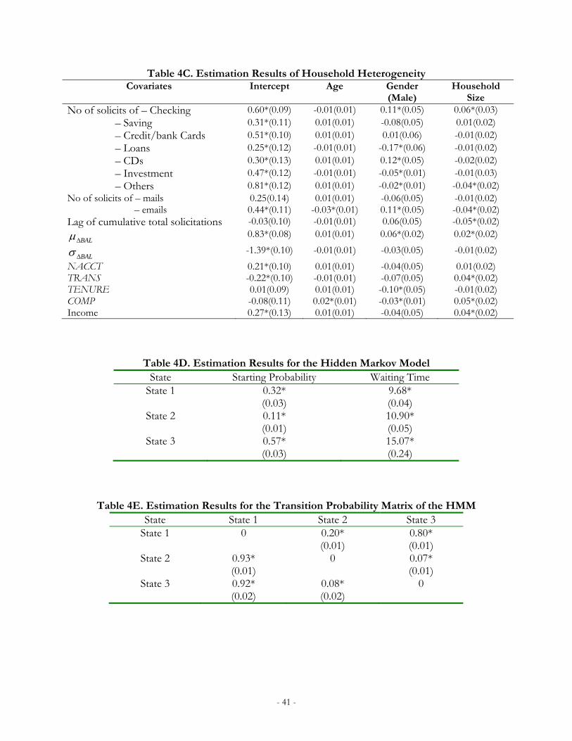
- 41 -

Table 4C. Estimation Results of Household Heterogeneity Covariates Intercept Age Gender

(Male) Household

Size No of solicits of – Checking 0.60*(0.09) -0.01(0.01) 0.11*(0.05) 0.06*(0.03) – Saving 0.31*(0.11) 0.01(0.01) -0.08(0.05) 0.01(0.02) – Credit/bank Cards 0.51*(0.10) 0.01(0.01) 0.01(0.06) -0.01(0.02) – Loans 0.25*(0.12) -0.01(0.01) -0.17*(0.06) -0.01(0.02) – CDs 0.30*(0.13) 0.01(0.01) 0.12*(0.05) -0.02(0.02) – Investment 0.47*(0.12) -0.01(0.01) -0.05*(0.01) -0.01(0.03) – Others 0.81*(0.12) 0.01(0.01) -0.02*(0.01) -0.04*(0.02) No of solicits of – mails 0.25(0.14) 0.01(0.01) -0.06(0.05) -0.01(0.02) – emails 0.44*(0.11) -0.03*(0.01) 0.11*(0.05) -0.04*(0.02) Lag of cumulative total solicitations -0.03(0.10) -0.01(0.01) 0.06(0.05) -0.05*(0.02)

BAL 0.83*(0.08) 0.01(0.01) 0.06*(0.02) 0.02*(0.02)

BAL -1.39*(0.10) -0.01(0.01) -0.03(0.05) -0.01(0.02)

NACCT 0.21*(0.10) 0.01(0.01) -0.04(0.05) 0.01(0.02) TRANS -0.22*(0.10) -0.01(0.01) -0.07(0.05) 0.04*(0.02) TENURE 0.01(0.09) 0.01(0.01) -0.10*(0.05) -0.01(0.02) COMP -0.08(0.11) 0.02*(0.01) -0.03*(0.01) 0.05*(0.02) Income 0.27*(0.13) 0.01(0.01) -0.04(0.05) 0.04*(0.02)

Table 4D. Estimation Results for the Hidden Markov Model State Starting Probability Waiting Time

State 1 0.32* (0.03)

9.68* (0.04)

State 2 0.11* (0.01)

10.90* (0.05)

State 3 0.57* (0.03)

15.07* (0.24)

Table 4E. Estimation Results for the Transition Probability Matrix of the HMM State State 1 State 2 State 3

State 1 0 0.20* (0.01)

0.80* (0.01)

State 2 0.93* (0.01)

0 0.07* (0.01)

State 3 0.92* (0.02)

0.08* (0.02)

0

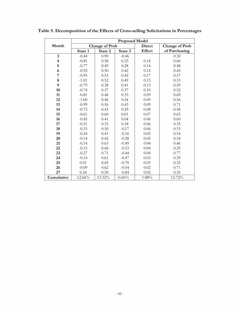
- 42 -

Table 5. Decomposition of the Effects of Cross-selling Solicitations in Percentages

Month

Proposed Model Change of Prob Direct

Effect Change of Prob of Purchasing State 1 State 2 State 3

3 4 5 6 7 8 9 10 11 12 13 14 15 16 17 18 19 20 21 22 23 24 25 26 27

-0.44 -0.81 -0.77 -0.92 -0.95 -1.01 -0.79 -0.74 -0.81 -1.00 -0.99 -0.72 -0.61 -0.45 -0.51 -0.33 -0.24 -0.14 -0.14 -0.15 -0.27 -0.14 0.01 -0.09 0.34

0.90 0.58 0.49 0.50 0.53 0.52 0.38 0.37 0.48 0.46 0.56 0.43 0.60 0.41 0.33 0.50 0.41 0.42 0.63 0.68 0.71 0.61 0.69 0.62 0.50

-0.46 0.23 0.28 0.42 0.42 0.49 0.41 0.37 0.33 0.54 0.43 0.29 0.01 0.04 0.18 -0.17 -0.16 -0.28 -0.49 -0.53 -0.44 -0.47 -0.70 -0.54 -0.84

0.14 0.14 0.12 0.17 0.15 0.13 0.10 0.09 0.09 0.09 0.08 0.07 0.06 0.06 0.06 0.05 0.05 0.04 0.04 0.04 0.03 0.03 0.02 0.02

0.30 0.66 0.48 0.45 0.57 0.33 0.59 0.52 0.69 0.56 0.71 0.58 0.65 0.60 0.33 0.33 0.54 0.54 0.46 0.25 0.77 0.39 0.35 0.71 0.35

Cumulative -12.66% 13.32% -0.66% 1.88% 12.72%

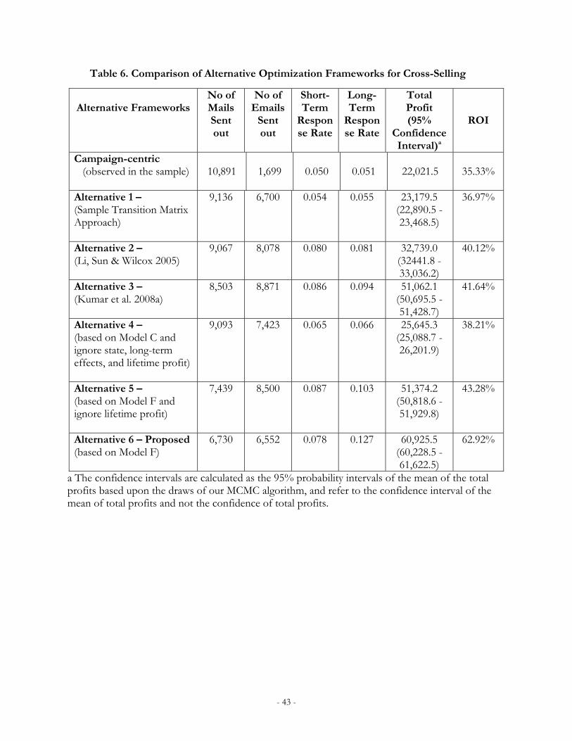
- 43 -

Table 6. Comparison of Alternative Optimization Frameworks for Cross-Selling

a The confidence intervals are calculated as the 95% probability intervals of the mean of the total profits based upon the draws of our MCMC algorithm, and refer to the confidence interval of the mean of total profits and not the confidence of total profits.

Alternative Frameworks

No of Mails Sent out

No of Emails

Sent out

Short-Term

Response Rate

Long-Term

Response Rate

Total Profit (95%

Confidence Interval)a

ROI

Campaign-centric (observed in the sample)

10,891

1,699

0.050

0.051

22,021.5

35.33%

Alternative 1 – (Sample Transition Matrix Approach)

9,136 6,700 0.054 0.055 23,179.5 (22,890.5 -23,468.5)

36.97%

Alternative 2 – (Li, Sun & Wilcox 2005)

9,067 8,078 0.080 0.081 32,739.0 (32441.8 - 33,036.2)

40.12%

Alternative 3 – (Kumar et al. 2008a)

8,503 8,871 0.086 0.094 51,062.1 (50,695.5 -51,428.7)

41.64%

Alternative 4 – (based on Model C and ignore state, long-term effects, and lifetime profit)

9,093 7,423 0.065 0.066 25,645.3 (25,088.7 -26,201.9)

38.21%

Alternative 5 – (based on Model F and ignore lifetime profit)

7,439 8,500 0.087 0.103 51,374.2 (50,818.6 -51,929.8)

43.28%

Alternative 6 – Proposed (based on Model F)

6,730 6,552 0.078 0.127 60,925.5 (60,228.5 -61,622.5)

62.92%

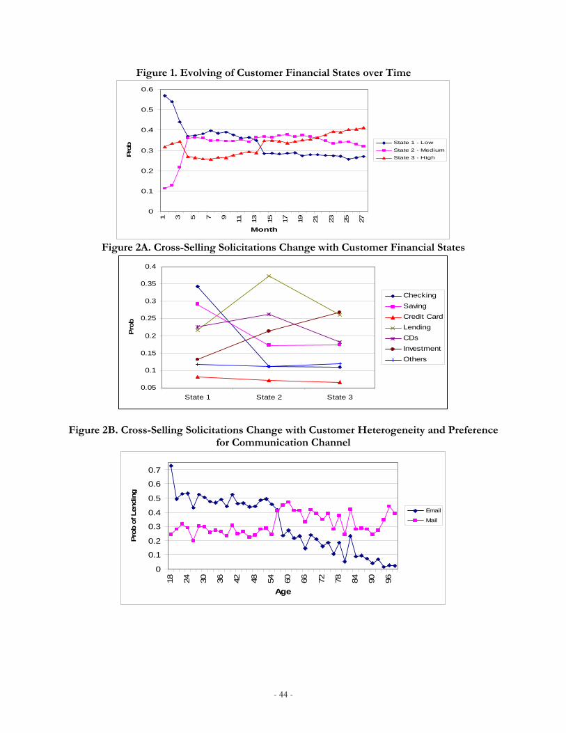
- 44 -

Figure 1. Evolving of Customer Financial States over Time

Figure 2A. Cross-Selling Solicitations Change with Customer Financial States

Figure 2B. Cross-Selling Solicitations Change with Customer Heterogeneity and Preference for Communication Channel

0

0.1

0.2

0.3

0.4

0.5

0.6

1 3 5 7 9

11

13

15

17

19

21

23

25

27

Month

Pro

b State 1 - Low

State 2 - Medium

State 3 - High

0.05

0.1

0.15

0.2

0.25

0.3

0.35

0.4

State 1 State 2 State 3

Pro

b

Checking

Saving

Credit Card

Lending

CDs

Investment

Others

0

0.1

0.2

0.3

0.4

0.5

0.6

0.7

18 24 30 36 42 48 54 60 66 72 78 84 90 96

Age

Pro

b o

f Len

din

g

Email

Mail

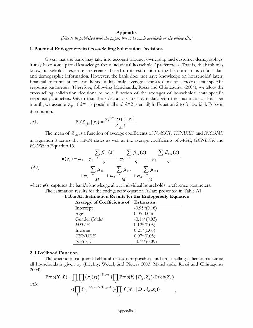
- Appendix 1 -

Appendix (Not to be published with the paper, but to be made available on the online site.)

1. Potential Endogeneity in Cross-Selling Solicitation Decisions

Given that the bank may take into account product ownership and customer demographics, it may have some partial knowledge about individual households’ preferences. That is, the bank may know households’ response preferences based on its estimation using historical transactional data and demographic information. However, the bank does not have knowledge on households’ latent financial maturity states and hence it has only average estimates on households’ state-specific response parameters. Therefore, following Manchanda, Rossi and Chintagunta (2004), we allow the cross-selling solicitation decisions to be a function of the averages of households’ state-specific response parameters. Given that the solicitations are count data with the maximum of four per month, we assume ijktZ ( k=1 is postal mail and k=2 is email) in Equation 2 to follow i.i.d. Poisson

distribution.

(A1) exp( )

Pr( | )!

ijktZ

i iijkt i

ijkt

ZZ

The mean of ijktZ is a function of average coefficients of NACCT, TENURE, and INCOME

in Equation 3 across the HMM states as well as the average coefficients of AGE, GENDER and HSIZE in Equation 13.

(A2)

6 8 10

0 1 2 3

1 2 3

4 5 6

( ) ( ) ( )ln( )

i i is s s

i

m m mm m m

s s s

S S S

M M M

where ’s captures the bank’s knowledge about individual households’ preference parameters. The estimation results for the endogeneity equation A2 are presented in Table A1.

Table A1. Estimation Results for the Endogeneity Equation Average of Coefficients of Estimates Intercept -0.95*(0.16) Age

0.05(0.03)

Gender (Male) -0.16*(0.03) HSIZE 0.12*(0.05) Income 0.21*(0.05) TENURE 0.07*(0.03) NACCT -0.34*(0.09)

2. Likelihood Function The unconditional joint likelihood of account purchase and cross-selling solicitations across all households is given by (Liechty, Wedel, and Pieters 2003; Manchanda, Rossi and Chintagunta 2004):

(A3) 0

( 1)

I{ }

I{ & }

Prob( , ) ( ) { Prob( | , ) Pr ob( )

( ) ( | , , )}

i

it i t

D s

i it it it iti s t

D s D litsl itk it it i

l k

s Y D Z Z

P f W D

Y Z

,

- Appendix 2 -

where Y is the whole observed choice sequence and Z is the observed cross-selling solicitations across households, products, and time, πi is the starting probability at time 0, and itslP is the transition probability from state s to l at time t defined in the HMM process. I{} is an indicator function. Prob(Zit) is the likelihood of observed cross-selling solicitations. Dit is the realized latent financial state for household i at time t. ( | , , )itk it it if W D is the density of the k-th waiting time of

household i at time t conditional on the realized hidden state itD and Gamma shape and scale

parameters it and i , which is given by

(A4)

( )( ) 1

0

1

( | , , ) ( ( ) ) exp{ ( ( ) )}( ( ))

I{ ( ) }

ik it

ik it

DDi

itk it it i k itk it k m i itk it k mm ik it

k m itk it k m

f W D W D W DD

W D

.

Here )( itik D is the Gamma shape parameter associated with the state of a household when the k-th

jump time begins and with the realized state D at time t, and mk is the m-th time after k – the k-th

jump time of the household – that D changed states, with 00 k . k is a normalizing constant of the density. Normalization and Identification For identification purposes, the diagonal elements of are normalized to 1 and hence becomes a correlation matrix. To ensure identification of the hidden states, we restrict the average purchase probabilities across all the products to be non-decreasing in the states (Li, Sun, and Wilcox 2005; Montgomery et al. 2004; Netzer, Lattin, and Srinivasan 2008). Since both the intercepts and the response parameters are state-specific, we impose this restriction at the mean of the vector of covariates. Thus, the covariates are mean-centered and the restrictions are imposed as

(A5) J

S

JJ

J

jij

J

jij

J

jij

10

10

10 )()2()1(

.

We also refer readers interested in the estimation procedure to Allenby and Rossi (1999), Gelfand and Smith (1990), Liechty, Wedel, and Pieters (2003), and Manchanda, Ansari, and Gupta (1999).

3. Modeling Expected Account Balance

Given that the bank and households do not know the future balance, we simply assume that for products household i already own at time t, the expected balance (expressed in thousands of dollars) in each account is exogenously given by the following equation11:

(A6) 0 1 ( 1) 2 ( 1) 3 ( 1)

1

4 51 1 1

ijt i i ij t i i t i i t

K J t

i it i ijk ijtk j

BAL BAL TENURE TRANS

COMP Z

,

11 Alternatively, we can develop a hidden Markov model to explain the balance in each account. Given our focus on customer responsiveness to a bank’s cross-selling campaign, we prefer to model purchase decision. Future research can incorporate balance decision to more accurately calculate customer lifetime value.

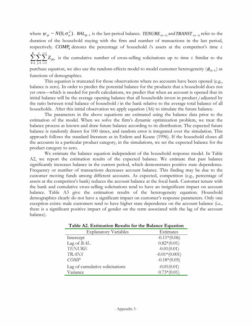
- Appendix 3 -

where ) ,0(~ 2 Nijt . 1ijtBAL is the last-period balance. )1( tiTENURE and )1( tiTRANST refer to the

duration of the household staying with the firm and number of transactions in the last period, respectively. itCOMP denotes the percentage of household i’s assets at the competitor’s time t.

K

k

J

j

t

ijkZ1 1

1

1 is the cumulative number of cross-selling solicitations up to time t. Similar to the

purchase equation, we also use the random-effects model to model customer heterogeneity ( 50i ) as functions of demographics. This equation is truncated for those observations where no accounts have been opened (e.g., balance is zero). In order to predict the potential balance for the products that a household does not yet own—which is needed for profit calculations, we predict that when an account is opened that its initial balance will be the average opening balance that all households invest in product j adjusted by the ratio between total balance of household i in the bank relative to the average total balance of all households. After this initial observation we apply equation (A6) to simulate the future balance. The parameters in the above equations are estimated using the balance data prior to the estimation of the model. When we solve the firm’s dynamic optimization problem, we treat the balance process as known and draw future balance according to its distribution. The expected future balance is randomly drawn for 100 times, and random error is integrated over the simulation. This approach follows the standard literature as in Erdem and Keane (1996). If the household closes all the accounts in a particular product category, in the simulations, we set the expected balance for the product category to zero.

We estimate the balance equation independent of the household response model. In Table A2, we report the estimation results of the expected balance. We estimate that past balance significantly increases balance in the current period, which demonstrates positive state dependence. Frequency or number of transactions decreases account balance. This finding may be due to the customer moving funds among different accounts. As expected, competition (e.g., percentage of assets at the competitor’s bank) reduces the account balance at the focal bank. Customer tenure with the bank and cumulative cross-selling solicitations tend to have an insignificant impact on account balance. Table A3 give the estimation results of the heterogeneity equation. Household demographics clearly do not have a significant impact on customer’s response parameters. Only one exception exists: male customers tend to have higher state dependence on the account balance (i.e., there is a significant positive impact of gender on the term associated with the lag of the account balance).

Table A2. Estimation Results for the Balance Equation Explanatory Variables Estimates

Intercept -0.11*(0.06) Lag of BAL 0.82*(0.01) TENURE -0.01(0.01) TRANS -0.01*(0.001) COMP -0.18*(0.05) Lag of cumulative solicitations -0.01(0.01) Variance 0.73*(0.01)

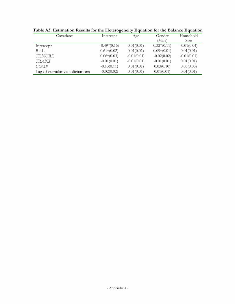
- Appendix 4 -

Table A3. Estimation Results for the Heterogeneity Equation for the Balance Equation Covariates Intercept Age Gender

(Male) Household

Size Intercept -0.49*(0.15) 0.01(0.01) 0.32*(0.11) -0.01(0.04) BAL 0.61*(0.02) 0.01(0.01) 0.09*(0.01) 0.01(0.01) TENURE 0.06*(0.03) -0.01(0.01) -0.02(0.02) -0.01(0.01) TRANS -0.01(0.01) -0.01(0.01) -0.01(0.01) 0.01(0.01) COMP -0.13(0.11) 0.01(0.01) 0.03(0.10) 0.03(0.03) Lag of cumulative solicitations -0.02(0.02) 0.01(0.01) 0.01(0.01) 0.01(0.01)