coupling of an individual-based model of anchovy with

Instructions for use

Title Coupling of an individual-based model of anchovy with lower trophic level and hydrodynamic models

Author(s) Yuheng, Wang; Hao, Wei; Kishi, Michio J.

Citation Journal of Ocean University of China, 12(1), 45-52https://doi.org/10.1007/s11802-013-1901-x

Issue Date 2013-03

Doc URL http://hdl.handle.net/2115/52116

Rights The original publication is available at www.springerlink.com

Type article (author version)

File Information JOUC12-1_45-52.pdf

Hokkaido University Collection of Scholarly and Academic Papers : HUSCAP

https://eprints.lib.hokudai.ac.jp/dspace/about.en.jsp

Coupling of an Individual-based Model of Anchovy with Lower

Trophic Level and Hydrodynamic Models

Wang Yuheng1), Wei Hao2), and Michio J. Kishi3)

1) Key Laboratory of Physical Oceanography, Ocean University of China, Qingdao 266100, P.R.

China

2) College of Marine Science and Engineering, Tianjin University of Science and Technology,

Tianjin 300457, P.R. China

3) Faculty of Fisheries Sciences, Hokkaido University, Hokkaido 060-0813, Japan

Abstract Anchovy (Engraulis japonicus)，a small pelagic fish and food of other economic fishes,

is a key species in the Yellow Sea ecosystem. Understanding the mechanisms of its recruitment and

biomass variation is important for the prediction and management of fishery resources. Coupled

with a hydrodynamic model (POM) and a lower trophic level ecosystem model (NEMURO), an

individual-based model of anchovy is developed to study the influence of physical environment on

anchovy’s biomass variation. Seasonal variations of circulation, water temperature and mix-layer

depth from POM are used as external forcing for NEMURO and the anchovy model. Biomasses of

large zooplankton and predatory zooplankton which anchovy feeds on are output from NEMURO

and are controlled by the consumption of anchovy on them. Survival fitness theory related to

temperature and food is used to determine the swimming action of anchovy in the model. The

simulation results agree well with observations and elucidate the influence of temperature in

over-wintering migration and food in feeding migration.

Key words anchovy; individual-based model; population dynamics; Yellow Sea

1 Introduction

Understanding the effect of physical environment on ecosystems is essential for developing

quantitative approaches to sustainable fishery management. The physical environment can influence

fish population by modifying lower trophic levels, altering fish bioenergetics and changing

migration routes. Many efforts have been made to establish end-to-end ecosystem models (Megrey

et al., 2007; Ito et al., 2007; Fulton, 2010) that make it possible to study the first and second effects

mentioned above. IBM (Individual-Based Model) models were developed to study saury’s response

to the climate variation in the north Pacific (Ito et al., 2007). However, most of these models use a

fixed migration route. While several migration models were built (Okunishi et al., 2009; Pershing et

al., 2009), they were not coupled with lower trophic level models. In this study, an individual-based

model is developed and coupled with low trophic level and hydrodynamic models for studying the

influence of physical environment on anchovy population in the Yellow Sea (YS).

The YS, a semi-enclosed shelf sea in the North Pacific, provides a major over-wintering and

feeding ground for numerous species of fish (Fig.1). The physical setting in the YS exhibits

complicated spatial and temporal variations. In winter, a warm and salty water mass is present in the

deep central trough. In summer, the deep layer below the thermocline is occupied by the Yellow Sea

Cold Water, thus providing an over-summering site for many temperate species. The water

temperature records in the YS suggest a regime shift occurring around 1986 (Wei et al., 2010). But

the influence of this change on the ecosystem remains unknown.

Anchovy (Engraulis japonius) is a widely distributed pelagic fish species living in temperate seas.

Before the initiation of a large-scale anchovy-targeted fishery in the early 1990s, anchovy was the

most abundant fish species in the YS with a stock of around 3 million tons (Zhu and Iversen, 1990).

Anchovy is important both as a prey species and as a major plankton feeder, hence plays a key role

in the ecosystem of the YS (Wei and Jiang, 1992). Anchovy is also one of the extensively studied

fish species in the YS. Studies on anchovy are important for the acquisition of bioenergetics

parameters.

Fig.1 The study area with depth contours (m).

2 Model description

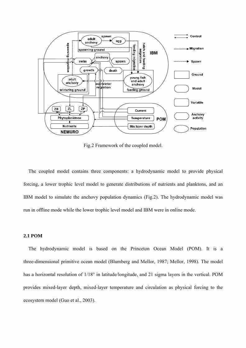
Fig.2 Framework of the coupled model.

The coupled model contains three components: a hydrodynamic model to provide physical

forcing, a lower trophic level model to generate distributions of nutrients and planktons, and an

IBM model to simulate the anchovy population dynamics (Fig.2). The hydrodynamic model was

run in offline mode while the lower trophic level model and IBM were in online mode.

2.1 POM

The hydrodynamic model is based on the Princeton Ocean Model (POM). It is a

three-dimensional primitive ocean model (Blumberg and Mellor, 1987; Mellor, 1998). The model

has a horizontal resolution of 1/18° in latitude/longitude, and 21 sigma layers in the vertical. POM

provides mixed-layer depth, mixed-layer temperature and circulation as physical forcing to the

ecosystem model (Guo et al., 2003).

2.2 NEMURO

NEMURO (the North Pacific Ecosystem Model Used for Regional Oceanography) is a low

trophic level ecosystem model developed by the model Task Team of the PICES CCCC (the North

Pacific Marine Science Organization, Climate Change and Carrying Capacity) program (Kishi et al.,

2007). It contains 11 state variables, including two kinds of phytoplankton (small phytoplankton, PS

and large phytoplankton, PL) and three kinds of zooplankton (small zooplankton, ZS, large

zooplankton, ZL, and predatory zooplankton, ZP). The model was originally used for the open

ocean (North Pacific). The following modifications of the model were made for the YS. 1) The

cycle of phosphate (HPO4-P, DOP (dissolved organic phosphorus) and POP (particulate organic

phosphorus)) was added (Wang, 2007) considering that the growth of phytoplankton in the YS is

mainly P-limited (Gao et al., 2004). 2) River and atmospheric inputs, the important sources of

nutrients, were added. 3) The method proposed by Wei et al. (2002) was used to calculate the

exchange of nutrients with the deeper ocean layer instead of using the fixed exchange rate in the

original NEMURO. 4) The suspended particulate matter (SPM) was taken into account in the

calculation of light intensity because of the high concentration of SPM in the YS.

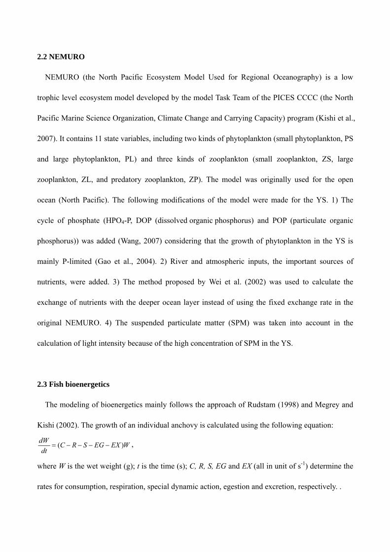
2.3 Fish bioenergetics

The modeling of bioenergetics mainly follows the approach of Rudstam (1998) and Megrey and

Kishi (2002). The growth of an individual anchovy is calculated using the following equation:

( )dW

C R S EG EX Wdt

,

where W is the wet weight (g); t is the time (s); C, R, S, EG and EX (all in unit of s-1) determine the

rates for consumption, respiration, special dynamic action, egestion and excretion, respectively. .

2.4 Population dynamics model

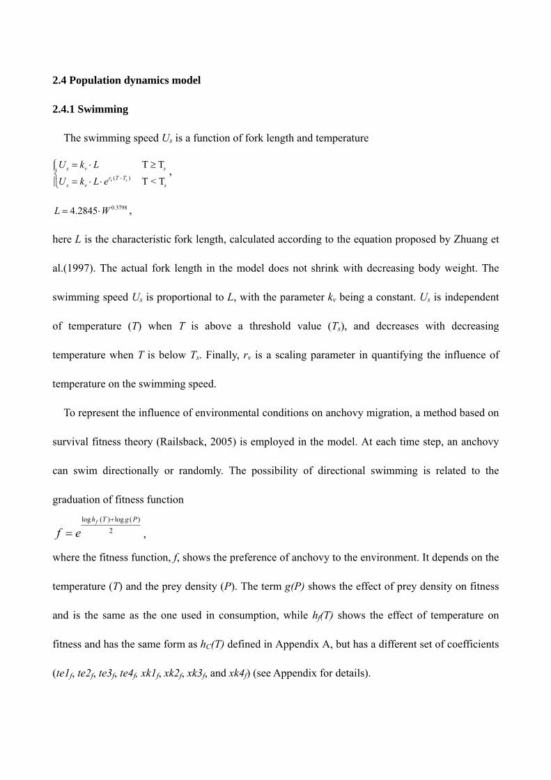
2.4.1 Swimming

The swimming speed Us is a function of fork length and temperature

( )

T T

T < Tv s

s v s

r T Ts v s

U k L

U k L e

,

0.37984.2845L W ,

here L is the characteristic fork length, calculated according to the equation proposed by Zhuang et

al.(1997). The actual fork length in the model does not shrink with decreasing body weight. The

swimming speed Us is proportional to L, with the parameter kv being a constant. Us is independent

of temperature (T) when T is above a threshold value (Ts), and decreases with decreasing

temperature when T is below Ts. Finally, rv is a scaling parameter in quantifying the influence of

temperature on the swimming speed.

To represent the influence of environmental conditions on anchovy migration, a method based on

survival fitness theory (Railsback, 2005) is employed in the model. At each time step, an anchovy

can swim directionally or randomly. The possibility of directional swimming is related to the

graduation of fitness function

log ( ) log ( )

2fh T g P

f e

,

where the fitness function, f, shows the preference of anchovy to the environment. It depends on the

temperature (T) and the prey density (P). The term g(P) shows the effect of prey density on fitness

and is the same as the one used in consumption, while hf(T) shows the effect of temperature on

fitness and has the same form as hC(T) defined in Appendix A, but has a different set of coefficients

(te1f, te2f, te3f, te4f, xk1f, xk2f, xk3f, and xk4f) (see Appendix for details).

The swimming direction is decided by the following equation:

<

(0, 2 )

fh

h

fR

f f

frand R

f f

,

(0,1)R rand ,

where rand(a,b) generates a random number of uniform distribution in the interval (a,b); Δf is the

horizontal gradient of the fitness; θf is the direction of Δf , with exp( 1 )ff f and Δfh is the

half saturation of Δf.

2.4.2 Migration

The motion of anchovy is a combination of swimming and passive drifting with current, hence

1n n c s t nP P v v t

,

is sv U e

,

where nP

and 1nP

denote respectively the position of an anchovy at time step n and n+1, cv

is

the water velocity, sv

is the swimming velocity, and Δt is the time step.

2.4.3 Reproduction

Anchovy is a multiple spawning pelagic species, maturing at a body length of about 8-9cm. The

spawning season of anchovy extends from May to September. There are many spawn fields along

the coast, but anchovy can spawn in the entire YS if environmental conditions are suitable (Zhu and

Iversen, 1990; Zhao, 2006). In the model, anchovy will spawn 5 times from mid-May through

September. Each time the number of eggs is calculated with the following procedures.

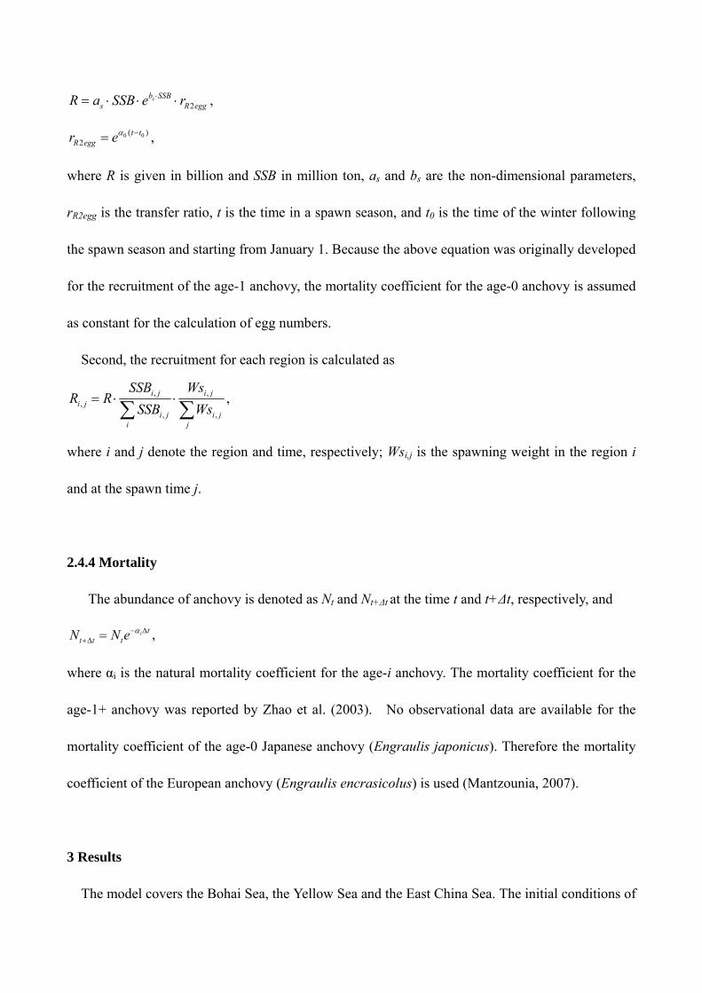
First, the total recruitment (R) is calculated as a function of spawning stock biomass (SSB)

according to Zhao et al. (2003), i.e.

2sb SSB

s R eggR a SSB e r ,

0 0( )2

t tR eggr e ,

where R is given in billion and SSB in million ton, as and bs are the non-dimensional parameters,

rR2egg is the transfer ratio, t is the time in a spawn season, and t0 is the time of the winter following

the spawn season and starting from January 1. Because the above equation was originally developed

for the recruitment of the age-1 anchovy, the mortality coefficient for the age-0 anchovy is assumed

as constant for the calculation of egg numbers.

Second, the recruitment for each region is calculated as

, ,,

, ,

i j i ji j

i j i ji j

SSB WsR R

SSB Ws

,

where i and j denote the region and time, respectively; Wsi,j is the spawning weight in the region i

and at the spawn time j.

2.4.4 Mortality

The abundance of anchovy is denoted as Nt and Nt+Δt at the time t and t+Δt, respectively, and

i tt t tN N e ,

where αi is the natural mortality coefficient for the age-i anchovy. The mortality coefficient for the

age-1+ anchovy was reported by Zhao et al. (2003). No observational data are available for the

mortality coefficient of the age-0 Japanese anchovy (Engraulis japonicus). Therefore the mortality

coefficient of the European anchovy (Engraulis encrasicolus) is used (Mantzounia, 2007).

3 Results

The model covers the Bohai Sea, the Yellow Sea and the East China Sea. The initial conditions of

nutrients and planktons are taken from the Marine Atlas of the Bohai Sea, Yellow Sea and East

China Sea (Editorial Board for Marine Atlas, 1991a, b). The values of the state variables (i.e.

planktons and nutrients) at lateral open boundaries are fixed, being set the same as the initial

conditions. This boundary specification is acceptable, because the open boundaries (at 130.61°E

and 24.08°N) are far away from the study area. For simulations, 500 schools of anchovy are put into

the model on January 1, each representing 6×108 anchovy. All the anchovy are supposed to be born

on June 15 the previous year and are randomly distributed in the over-wintering ground. The model

simulation was run for 9 years and the results for the last 4 years were analyzed.

3.1 Growth

Fig. 3 The growth of anchovy as a function of (a) wet weight (g) and (b) total length (cm). The

model results and observations are represented by solid lines and different symbols, respectively.

The growth of anchovy from model simulation and observations are shown in Fig. 3Fig. 3. The

model results and observations are in good agreement except for the age-1 anchovy, both the

calculated weight and total length of which are less than the observed values. There are two

possible reasons for this discrepancy. First, some parameters for the age-1 anchovy are used in the

place of the parameters for the age-0 anchovy because the later are unknown. Secondly, most of the

observational data were collected from the over-wintering ground, the observations may

overestimate the growth. Jin et al. (2005) reported the existence of the age-0 anchovy in the Bohai

Sea in December. This suggests that anchovy with low swimming ability (usually with shorter total

lengths and lighter weights) may not have been included in the datasets collected in over-wintering

grounds (Zhao, 2006).

3.2 Age structure

Fig. 4 The calculated age structure of the over-wintering stock.

Fig. 5 The age structure of spawning stock from (a) observations (Li et al., 2006) and (b) model

results.

Zhao (2006) analyzed the observed age structure of the over-wintering stocks from 1985 through

2005 and found a significant difference between those before and after the collapse of anchovy

population in the late 1990s. As fishing is not taken into account in this model, only the data before

the late 1990s are used. During this period, the age-1 anchovy accounts for 30%-60% of the

spawning stock, the age-2 20%-50%, the age-3 10%-30%, and the age-4 less than 10%. The model

results (Fig. 4Fig. 4) agrees with the observed values fairly well. The modeled age structure of the

spawning stock in to the south of the Shandong Peninsula in the YS (Fig. 5b) generally agrees with

the observed structure reported by Li et al. (2006) (Fig. 5a).

3.3 Migration

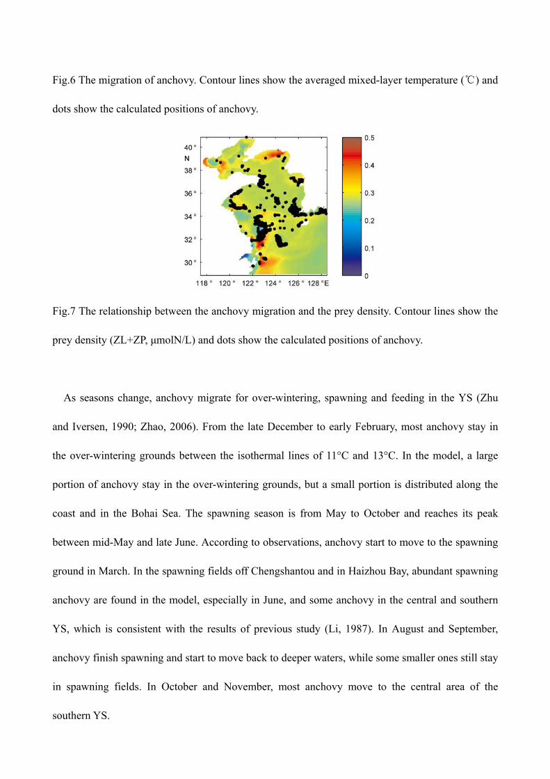
Fig.6 The migration of anchovy. Contour lines show the averaged mixed-layer temperature (℃) and

dots show the calculated positions of anchovy.

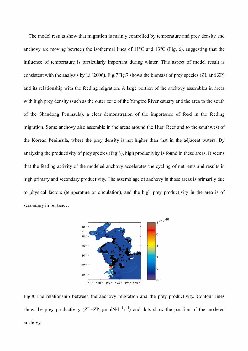
Fig.7 The relationship between the anchovy migration and the prey density. Contour lines show the

prey density (ZL+ZP, μmolN/L) and dots show the calculated positions of anchovy.

As seasons change, anchovy migrate for over-wintering, spawning and feeding in the YS (Zhu

and Iversen, 1990; Zhao, 2006). From the late December to early February, most anchovy stay in

the over-wintering grounds between the isothermal lines of 11°C and 13°C. In the model, a large

portion of anchovy stay in the over-wintering grounds, but a small portion is distributed along the

coast and in the Bohai Sea. The spawning season is from May to October and reaches its peak

between mid-May and late June. According to observations, anchovy start to move to the spawning

ground in March. In the spawning fields off Chengshantou and in Haizhou Bay, abundant spawning

anchovy are found in the model, especially in June, and some anchovy in the central and southern

YS, which is consistent with the results of previous study (Li, 1987). In August and September,

anchovy finish spawning and start to move back to deeper waters, while some smaller ones still stay

in spawning fields. In October and November, most anchovy move to the central area of the

southern YS.

The model results show that migration is mainly controlled by temperature and prey density and

anchovy are moving bewteen the isothermal lines of 11°C and 13°C (Fig. 6), suggesting that the

influence of temperature is particularly important during winter. This aspect of model result is

consistent with the analysis by Li (2006). Fig.7Fig.7 shows the biomass of prey species (ZL and ZP)

and its relationship with the feeding migration. A large portion of the anchovy assembles in areas

with high prey density (such as the outer zone of the Yangtze River estuary and the area to the south

of the Shandong Peninsula), a clear demonstration of the importance of food in the feeding

migration. Some anchovy also assemble in the areas around the Hupi Reef and to the southwest of

the Korean Peninsula, where the prey density is not higher than that in the adjacent waters. By

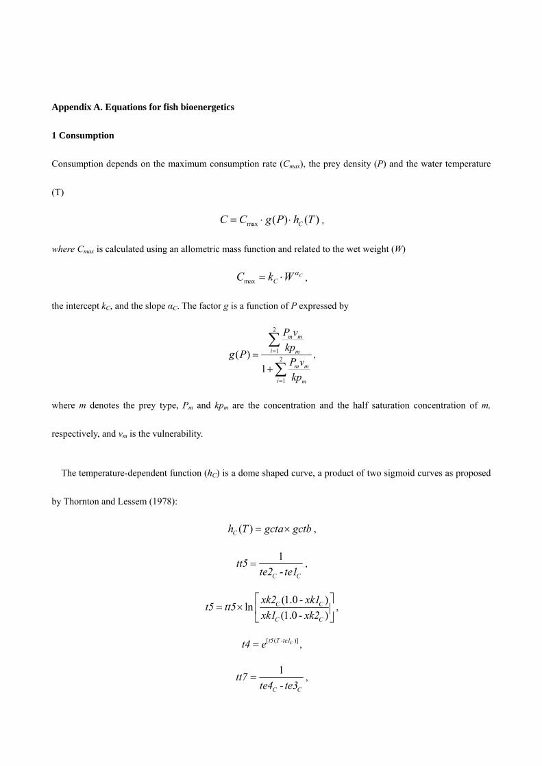
analyzing the productivity of prey species (Fig.8), high productivity is found in these areas. It seems

that the feeding activity of the modeled anchovy accelerates the cycling of nutrients and results in

high primary and secondary productivity. The assemblage of anchovy in those areas is primarily due

to physical factors (temperature or circulation), and the high prey productivity in the area is of

secondary importance.

Fig.8 The relationship between the anchovy migration and the prey productivity. Contour lines

show the prey productivity (ZL+ZP, μmolN·L-1·s-1) and dots show the position of the modeled

anchovy.

4 Discussion and summary

An individual-based model for anchovy, coupled with a low trophic level model and a

hydrodynamic model, is developed and applied in the Yellow Sea. The model results of the growth

and age structure show a good agreement with observations. The calculated pattern of the anchovy

migration is also similar to that based on observations. The results suggest that water temperature is

an important factor for the over-wintering migration while food is important for the feeding

migration. Thus, it is essential to take both factors into account in a migration model.

Two issues remain to be resolved in the calculations. First, anchovy stay in the coastal area

during the winter time, which is inconsistent with observations. Adding salinity into the fitness

function may improve the model performance. Second, anchovy in the model seldom move through

the Bohai Strait, which could be due to the over simplification of the migration mechanism adopted

in the model. The modeled anchovy only perceive the environment at adjacent grids. If the

environment is favorable to anchovy inside the Bohai Sea but not at the Bohai Strait, the anchovy

outside will not migrate to the Bohai Sea through the Strait. Future resolution of those issues

requires further understanding of the anchovy migration mechanism.

Acknowledgements

This work was supported by the National Natural Science Foundation of China (Grant No.

40830854) and the National Basic Research Program of China (Grant No. 2011CB403606). We are

grateful to Prof. Guo Xinyu at Ehime University for providing POM output. We thank the four

anonymous reviewers for their comments and suggestions.

References

Blumberg A. F., and G. L. Mellor, 1987. A description of a three dimensional coastal ocean circulation model.

Three-Dimensional Coastal Ocean Models, N. Heaps, Ed., Coastal and Estuarine Series, No. 4, American

Geophysical Union, 1-16.

Editorial Board for Marine Atlas, 1991. Marine atlas of Bohai Sea, Yellow Sea and East China Sea (Chemistry).

Beijing: China Ocean Press (in Chinese).

Editorial Board for Marine Atlas, 1991. Marine atlas of Bohai Sea, Yellow Sea and East China Sea (Biology).

Beijing: China Ocean Press (in Chinese).

Fulton E. A., 2010. Approaches to end-to-end ecosystem models. Journal of Marine Systems, 81:171-183.

Gao S. Q., Y. A. Lin, M. M. Jin, and D. W. Gao, 2004. Distribution features of nutrients and nutrient structure in

the East China Sea and the Yellow Sea in spring and autumn. Donghai Marine Science, 22(4):38-50 (in

Chinese with English abstract).

Guo X. Y., H. Hukuda, Y. Miyazawa, and T. Yamagata, 2003. A Triply Nested Ocean Model for Simulating the

Kuroshio—Roles of Horizontal Resolution on JEBAR. Journal of Physical Oceanography, 33:146–169.

Ito S. I., B. A. Megrey, M. J. Kishi, D. Mukai, Y. Kurita, Y. Ueno, Y. Yamanaka, 2007. On the interannual

variability of the growth of Pacific saury (Cololabis saira): A simple 3-box model using NEMURO.FISH.

Ecological Modelling, 202:174-183

Jin X. S., X. Y. Zhao, and T. X. Meng, 2005. Biological resources and habitat environment of Bohai Sea and

Yellow Sea. Beijing: Science Press(in Chinese).

Kishi M. J., M. Kashiwai, D. M. Ware, B. A. Megrey, D. L. Eslinger, F. E. Werner, M. Noguchi-Aita, T.

Azumaya, M. Fujii, S. Hashimoto, D. J. Huang, H. Iizumi, Y. Ishida, S. Kang, G. A. Kantakov, H. Kim, K.

Komatsu, V. V. Navrotsky, S. L. Smith, K. Tadokoro, A. Tsuda, O. Yamamura, Y. Yamanaka, K. Yokouchi, N.

Yoshie, J. Zhang, Y. I. Zuenko, and V. I. Zvalinsky, 2007. NEMURO—a lower trophic level model for the

North Pacific marine ecosystem. Ecological Modelling, 202:12-25.

Li F. G.., 1987. Reproductive behavior of anchovy in middle and south Yellow Sea. Marine Fisheries Research,

8:41-50 (in Chinese).

Li X. S., X. Y. Zhao, F. Li, F. G. Li, Q. F. Dai, and J. C. Zhu, 2006. Structure and its variation of the anchovy

(Engraulis japonicus) spawning stock in the Southern waters to Shandong Peninsula. Marine Fisheries

Research, 27(1):46-53 (in Chinese with English abstract).

Li Y., 2006. Migration and Distribution of Anchovy in Yellow Sea and Its Relation with Environmental Factors.

Master Dissertation. Qingdao: Ocean University of China, (in Chinese with English abstract).

Mantzounia I., S. Somarakis, D. K. Moutopoulos, A. Kallianiotis, and C. Koutsikopoulos, 2007. Periodic,

spatially structured matrix model for the study of anchovy (Engraulis encrasicolus) population dynamics in N

Aegean Sea (E. Mediterranean). Ecological Modelling, 208:367-377.

Megrey B. A., and M. J. Kishi, 2002. Model/REX workshop to develop a marine ecosystem model of the North

Pacific Ocean including pelagic fishes. PICES Scientific Reports, 20:77–176.

Megrey B.A., K.A. Rose, R.A. Klumb, D.E. Hay, F.E. Werner, D.L. Eslinger, and S.L. Smith, 2007.

Bioenergetics-based population dynamics model of Pacific herring (Clupea harenguspallasii) coupled to a

lower trophic level nutrient–phytoplankton–zooplankton model: description, calibration and sensitivity analysis.

Ecological Modelling, 202: 144-164.

Mellor G. L., User’s guide for a three-dimensional, primitive equation, numerical ocean model. Rep., Program in

Atmospheric and Oceanic Science, Princeton University, 1998.

Okunishi T., Y. Yamanaka, and S. Ito, 2009. A simulation model for Japanese sardine (Sardinops melanostictus)

migrations in the western North Pacific. Ecological Modelling, 220: 462-479.

Pershing A. J., N. R. Record, B. C. Monger, C. A. Mayo, M. W. Brown, T. V. N. Cole, R. D. Kenney, D. E.

Pendleton, and L. A. Woodard, 2009. Model-based estimates of right whale habitat use in the Gulf of Maine.

Marine Ecology Progress Series, 378: 245-257.

Railsback S. F., B. C. Harvey, J. W. Hayse, and K. E. LaGory, 2005. Tests of theory for diel variation in salmonid

feeding activity and habitat use. Ecology, 86(4): 947-959.

Rudstam L. G., 1988. Exploring the dynamics of herring consumption in the Baltic: applications of an energetic

model of fish growth. Kieler Meeresforschung Sonderheft, 6:312–322.

Thornton, K. W., and A. S. Lessem, 1978. A temperature algorithm for modifying biological rates. Transactions

of the American Fisheries Society, 107(2):284–287.

Wang Z, 2007. Modeling and analysis of the change of plankton ecosystem in Jiaozhou Bay for 40 years. Master

Dissertation. Qingdao: Ocean University of China (in Chinese with English abstract).

Wei H., L. Wang, Y. A. Lin, and C. S. Chuang, 2002. Nutrient transport across the thermocline in the central

Yellow Sea. Advances in Marine Science, 20(3):15-20 (in Chinese with English abstract).

Wei H., J. Shi, Y. Lu, and Y. Peng, 2010. Interannual and long-term hydrographic changes in the Yellow Sea

during 1977-1998. Deep-Sea Research Part II, 57(11-12): 1025-1034.

Wei S., and W. M. Jiang, 1992. Study on food web of fishes in the Yellow Sea. Oceanologia Et Limnologia

Sinica, 23: 182-192 (in Chinese with English abstract).

Zhao X., J. Hamre, F. Li, X. Jin, and Q. Tang, 2003. Recruitment, sustainable yield and possible ecological

consequences of the sharp decline of the anchovy (Engraulis japonicus) stock in the Yellow Sea in the 1990s.

Fishery Oceanography, 12(4/5):495-501.

Zhao X. Y., 2006. Population dynamic characteristics and sustainable utilization of the anchovy stock in the

Yellow Sea. Doctor Dissertation. Qingdao: Ocean University of China (in Chinese with English abstract).

Zhu D. S., and S. A. Iversen, 1990. Anchovy and other fish resources in the Yellow Sea and East China Sea.

Marine Fishery Ressearch, 11: 1-143(in Chinese with English abstract).

Zhuang X. F., H. L. Jiang, and J. Lin, 1997. The relationship between parameters of anchovy body size and their

infect on drift net. Fisheries Science, 16(5):26-30 (in Chinese).

Appendix A. Equations for fish bioenergetics

1 Consumption

Consumption depends on the maximum consumption rate (Cmax), the prey density (P) and the water temperature

(T)

max ( ) ( )CC C g P h T ,

where Cmax is calculated using an allometric mass function and related to the wet weight (W)

maxC

CC k W ,

the intercept kC, and the slope αC. The factor g is a function of P expressed by

2

12

1

( )1

m m

i m

m m

i m

P v

kpg P

P v

kp

,

where m denotes the prey type, Pm and kpm are the concentration and the half saturation concentration of m,

respectively, and vm is the vulnerability.

The temperature-dependent function (hC) is a dome shaped curve, a product of two sigmoid curves as proposed

by Thornton and Lessem (1978):

( )Ch T gcta gctb ,

1

-C C

tt5te2 te1

,

(1.0 - )ln

(1.0 - )C C

C C

xk2 xk1t5 tt5

xk1 xk2

,

[ ( - )]Ct5 T te1t4 e ,

1

-C C

tt7te4 te3

,

(1.0 - )ln

(1.0 - )C C

C C

xk3 xk4t7 tt7

xk4 xk3

,

[ ( - )]Ct7 te4 Tt6 e ,

1.0 ( -1.0)C

C

xk1 t4gcta

xk1 t4

,

1.0 ( -1.0)C

C

xk4 t6gctb

xk4 t6

,

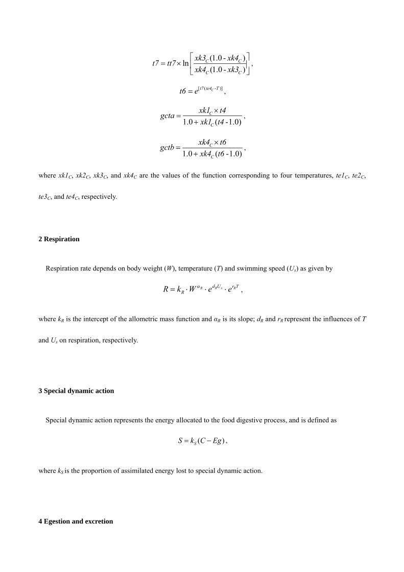
where xk1C, xk2C, xk3C, and xk4C are the values of the function corresponding to four temperatures, te1C, te2C,

te3C, and te4C, respectively.

2 Respiration

Respiration rate depends on body weight (W), temperature (T) and swimming speed (Us) as given by

R sR Rd U r TRR k W e e ,

where kR is the intercept of the allometric mass function and αR is its slope; dR and rR represent the influences of T

and Us on respiration, respectively.

3 Special dynamic action

Special dynamic action represents the energy allocated to the food digestive process, and is defined as

( )SS k C Eg ,

where kS is the proportion of assimilated energy lost to special dynamic action.

4 Egestion and excretion

Egestion is a constant proportion of consumption while excretion is a constant proportion of assimilated energy:

EgEg k C ,

( )ExEx k C Eg ,

where kEg and kEx are the scaling factors for egestion and excretion, respectively.

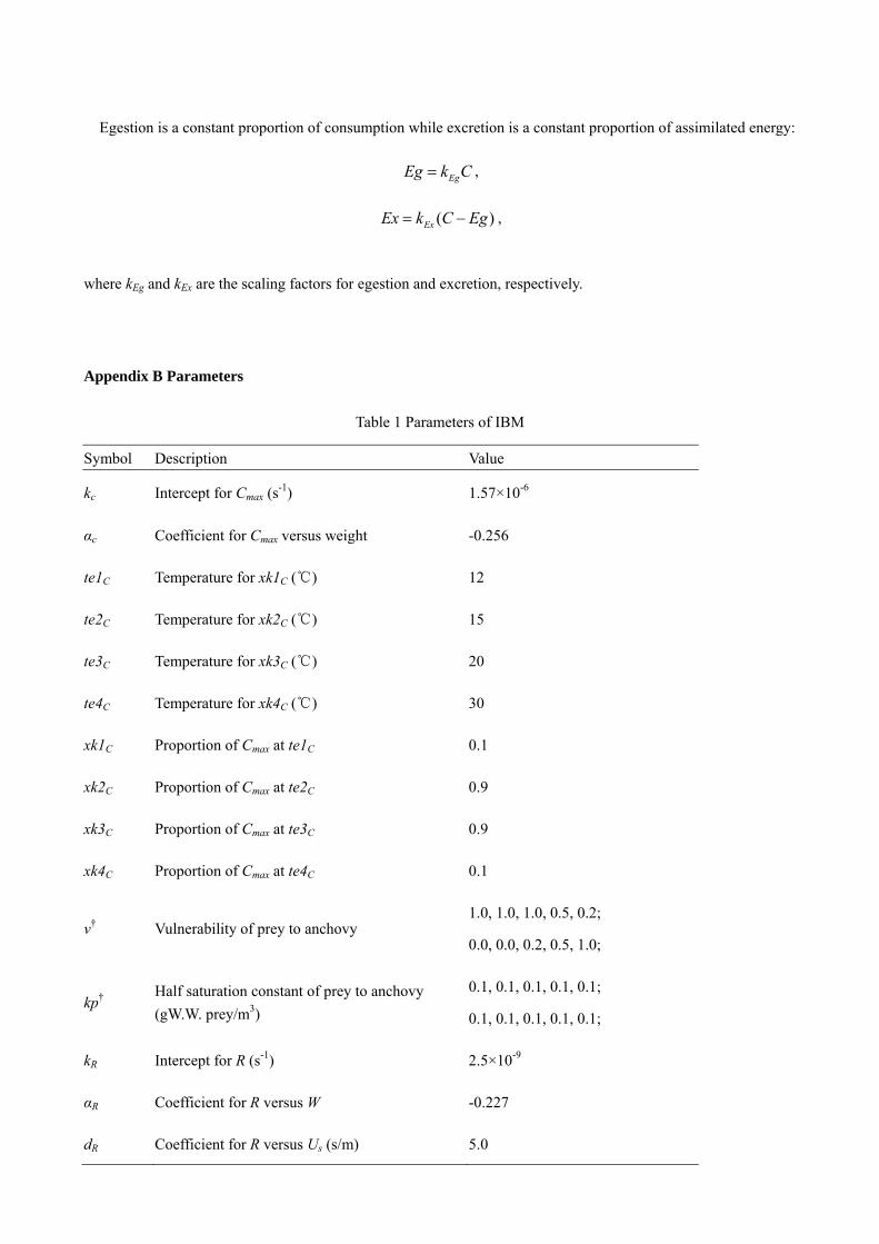
Appendix B Parameters

Table 1 Parameters of IBM

Symbol Description Value

kc Intercept for Cmax (s-1) 1.57×10-6

αc Coefficient for Cmax versus weight -0.256

te1C Temperature for xk1C (℃) 12




xk1C Proportion of Cmax at te1C 0.1




v† Vulnerability of prey to anchovy 1.0, 1.0, 1.0, 0.5, 0.2;

0.0, 0.0, 0.2, 0.5, 1.0;

kp† Half saturation constant of prey to anchovy

(gW.W. prey/m3)

0.1, 0.1, 0.1, 0.1, 0.1;

0.1, 0.1, 0.1, 0.1, 0.1;

kR Intercept for R (s-1) 2.5×10-9

αR Coefficient for R versus W -0.227

dR Coefficient for R versus Us (s/m) 5.0

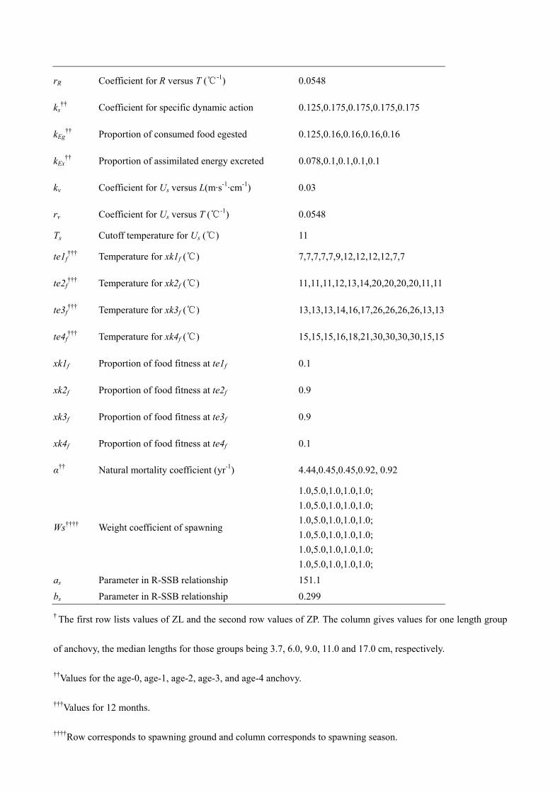
rR Coefficient for R versus T (℃-1) 0.0548

ks†† Coefficient for specific dynamic action 0.125,0.175,0.175,0.175,0.175

kEg†† Proportion of consumed food egested 0.125,0.16,0.16,0.16,0.16

kEx†† Proportion of assimilated energy excreted 0.078,0.1,0.1,0.1,0.1

kv Coefficient for Us versus L(m·s-1·cm-1) 0.03

rv Coefficient for Us versus T (℃-1) 0.0548

Ts Cutoff temperature for Us (℃) 11

te1f††† Temperature for xk1f (℃) 7,7,7,7,7,9,12,12,12,12,7,7




xk1f Proportion of food fitness at te1f 0.1




α†† Natural mortality coefficient (yr-1) 4.44,0.45,0.45,0.92, 0.92

Ws†††† Weight coefficient of spawning

1.0,5.0,1.0,1.0,1.0;

1.0,5.0,1.0,1.0,1.0;

1.0,5.0,1.0,1.0,1.0;

1.0,5.0,1.0,1.0,1.0;

1.0,5.0,1.0,1.0,1.0;

1.0,5.0,1.0,1.0,1.0;

as Parameter in R-SSB relationship 151.1

bs Parameter in R-SSB relationship 0.299

† The first row lists values of ZL and the second row values of ZP. The column gives values for one length group

of anchovy, the median lengths for those groups being 3.7, 6.0, 9.0, 11.0 and 17.0 cm, respectively.

††Values for the age-0, age-1, age-2, age-3, and age-4 anchovy.

†††Values for 12 months.

††††Row corresponds to spawning ground and column corresponds to spawning season.

coupling of an individual-based model of anchovy with

Documents