POLITECNICO DI MILANO

Facoltà di Ingegneria Industriale e dell’Informazione

Corso di Laurea in

Ingegneria Aeronautica

COLD WIRE THERMOMETRY

FOR TURBINE MEASUREMENTS

Relatore: Prof. Carlo Osnaghi

Co-relatore: Dr. Sergio Lavagnoli

Tesi di Laurea di:

Guido LATORRE Matr. 799309

Anno Accademico 2014-2015

II

III

Acknowledgements

IV

V

Contents

Acknowledgements ........................................................................................................ III

List of Figures ................................................................................................................. VII

List of tables ................................................................................................................. XIII

Abstract ........................................................................................................................ XIX

Key words: ................................................................................................................ XIX

Chapter 1: Introduction ................................................................................................... 1

1.1 Research and instrumentation for turbine measurements ................................... 1

1.2 Objectives of the work ........................................................................................... 3

1.3 Thesis Outline......................................................................................................... 4

Chapter 2: Experimental apparatus ................................................................................ 5

2.1 The turbine test rig ................................................................................................ 5

2.2 Setup for calibration of cold wires ......................................................................... 8

2.3 Support to set height and angle of probes ............................................................ 9

Chapter 3: Probes: working principle and calibration processes ................................ 11

3.1 Thermocouples .................................................................................................... 11

3.1.1 Errors and corrections................................................................................... 15

3.1.2 Thermocouples calibration process .............................................................. 18

3.2 Cold wires ............................................................................................................. 22

3.2.1 Cold wire static calibration (oven) ................................................................ 29

3.2.2 Cold wire static calibration (heated jet) ....................................................... 35

Chapter 4: Numerical Filtering and Signal Compensation ........................................... 45

4.1 Numerical filtering ............................................................................................... 46

4.1.1 Experimental Setup ....................................................................................... 46

4.1.2 Experimental Procedure to test Filter Box .................................................... 51

4.1.3 Post-processing of data ................................................................................. 52

4.1.4 Results ........................................................................................................... 57

4.1.5 Conclusions ................................................................................................... 66

4.2 Signal compensation ............................................................................................ 67

VI

4.2.1 Mathematical description of the problem .................................................... 67

Chapter 5: Experimental activity .................................................................................. 79

5.1 Dynamic calibration of the cold wire ................................................................... 79

5.1.1 Experimental setup ....................................................................................... 80

5.1.2 Step tests ....................................................................................................... 82

5.2 Compensation of the signal ................................................................................. 91

5.2.1 FFT ratio approach ........................................................................................ 92

5.2.2 Differentiation approach .............................................................................. 94

5.2.3 TFEST approach ............................................................................................. 96

5.2.4 Conclusions ................................................................................................. 103

5.3 Cold wire test in CT3 .......................................................................................... 104

5.3.1 Description of the test ................................................................................ 104

5.3.2 Experimental setup ..................................................................................... 105

5.3.3 Test and results ........................................................................................... 108

5.3.4 Compensation of the cold wire ................................................................... 111

5.3.5 Conclusions ................................................................................................. 117

Bibliography ................................................................................................................ 119

Appendix A – Results of the analogue filter ............................................................... 121

Appendix B – Setup for probes setting ....................................................................... 133

VII

List of Figures

Figure 1.1 Section view of the Rolls-Royce Trent 1000…………….…….1

Figure 2.1 The turbine test rig of Von Karman Institute………………….6

Figure 2.2 A schematic representation of CT3……………….................7

Figure 2.3 Setup for the calibration of cold wire…………………………8

Figure 2.4 Metallic supports……………………………………………. 9

Figure 2.5 Metallic tool designed in CATIA……………………………10

Figure 3.1 Configurations of thermocouples………..…………………..12

Figure 3.2 Electric polarity of metals function of temperature…………13

Figure 3.3 Characteristic curve of a thermocouple without

reference zone box..................................................................13

Figure 3.4 Thermocouple measurement with a reference box…………...14

Figure 3.5 Measurements with a reference zone

box-second configuration………………………………….. 14

Figure 3.6 Reference system for thermocouple steady errors…………. 16

Figure 3.7 Julabo 12-b oil-bath………………………………………… 19

Figure 3.8 Stabilization of temperature of cold wire…………………… 20

Figure 3.9 Table with calibration values of thermocouples……………. 20

Figure 3.10 Calibration curve of 4R thermocouple……………………… 21

Figure 3.11 Principle of resistance thermometer………………………… 22

Figure 3.12 The effect of convection (velocity) on the

cut-off frequency …………………………………………… 25

Figure 3.13 Particular of a cold wire: the wire is suspended between

two stain prongs…………………………………………….. 26

Figure 3.14 The effect of conduction on the prongs……………………. 27

VIII

Figure 3.15 Transfer function of the wire-prong system………………… 29

Figure 3.16 Cold wires DAO121A, DAO123A…………………………. 30

Figure 3.17 Setup for the static calibration in the oven…………………. 31

Figure 3.18 Schematic representation of the wiring of a cold wire……… 32

Figure 3.19 Stability of the white box TUCW2……................................. 33

Figure 3.20 Results of the static calibration in the oven of the two cold wires

DAO121A, DAO123A……………………………………… 34

Figure 3.21 Experimental setup for the static calibration of the cold wire in the

jet…………………………………………………………… 35

Figure 3.22 The cold wire boxes (Wheatstone bridge)………………….. 36

Figure 3.23 Setup for the calibration of the SENSYM (differential pressure

transducer)………………………………………………….. 37

Figure 3.24 Calibration curve of the SENSYM R4S4…………………... 38

Figure 3.25 Thermocouple 4R (up) and cold wire (put horizontally)…… 38

Figure 3.26 The heating system for the air pressurized reservoir……….. 39

Figure 3.27 Comparison of head 2A before and after reparation………... 43

Figure 4.1 Filter boxes………………………………………………….. 46

Figure 4.2 Electronic cards. The filter boxes are supplied by

electronic cards………………………………………………47

Figure 4.3 The frequency generator is used to produce signal of known shape

and frequency……………………………………………….. 48

Figure 4.4 GENESIS data acquisition system………………………….. 49

Figure 4.5 Experimental setup for filter boxes tests……………………. 51

Figure 4.6 The output of the acquisition obtained with Perception……. 52

Figure 4.7 The acquired sinusoidal signal is affected by noise that has to be

corrected…………………………………………………….. 53

Figure 4.8 The sinusoidal signal crosses the zero several times generating a

‘zero cloud’…………………………………………………. 54

IX

Figure 4.9 An example of cross-correlation……………………………. 55

Figure 4.10 The signal before and after having used the ‘smooth’ function in

Matlab………………………………………………………. 56

Figure 4.11 The Fast Fourier Transform of a signal allows to find the frequency

content of a signal…………………………………………... 56

Figure 4.12 High-Pass Gain………………………………………………58

Figure 4.23 Raw Phase shift…………………………………………….. 64

Figure 4.25 Example of a cold wire step signal…………………………..68

Figure 4.26 Configuration of a cold wire………………………………... 68

Figure 4.27 Comparison of the computed first order transfer function with the

one found by Dénos………………………………………… 71

Figure 4.28 Comparison between the computed two order transfer function

with the one found by Dénos……………………………….. 74

Figure 4.29 Comparison between the computed five first order transfer

function and the one obtained by Dénos……………………. 77

Figure 5.1 Physical characteristics and calibration coefficients of cold wire

DAO123A…………………………………………………... 81

Figure 5.2 Step test with calibration coefficients of the test done at Mach 0

……………………………………………………………… 83

Figure 5.3 Step test with calibration coefficients of the test done at Mach 0.05

……………………………………………………………… 84

Figure 5.4 Step test with calibration coefficients of the test done at Mach 0.05;

a shift has been subtracted to the cold wire signal………… 85

Figure 5.5 Step test 1 at Mach 0.05……………………………………. 86

Figure 5.6 Step test 1 at Mach 0.1……………………………………… 86

Figure 5.7 Step test 1 at Mach 0.2……………………………………… 87

Figure 5.8 Step test 1 at Mach 0.3……………………………………… 87

Figure 5.9 The setup used to realize the step tests……………………….88

Figure 5.10 Step test 2 at Mach 0.05………………………………………89

X

Figure 5.11 Step test 2 at Mach 0.1……………………………………….. 89

Figure 5.12 Step test 2 at Mach 0.2……………………………………….. 90

Figure 5.13 Step test 2 at Mach 0.3……………………………………… 90

Figure 5.14 Comparison between the cold wire step signal and the theoretical

Heaviside step………………………………………………. 93

Figure 5.15 Fast Fourier Transform of the cold wire signal (blue and the

Heaviside signal (red)………………………………………. 93

Figure 5.16 The ratio of the FFT of the cold wire signal and the FFT of the

Heaviside input signal gives the experimental transfer

function……………………………………………………... 94

Figure 5.17 The impulse has been obtained subtracting two consecutively

values of the original signal and dividing this value by the delta

time between them………………………………………….. 95

Figure 5.18 The resulting transfer function obtained after having redefined the

step impulse…………………………………………………. 96

Figure 5.19 The theoretical true step is the step generated by the movement of

the shield……………………………………………………. 97

Figure 5.20 The signal of the cold wire has been cleaned from spurious peaks,

low-pas filtered and adimensionalized……………………… 98

Figure 5.21 The experimental transfer functions found with ‘tfest’ with a

different number of poles, tested at Mach number 0.05……. 98

Figure 5.22 The modified transfer function combines the low frequency

behaviour of the experimental transfer function found with ‘tfest’

and the high frequency behaviour typical of the tungsten wire

………………………………………………………………. 100

Figure 5.23 The transfer functions found with ‘tfest’ imposing different

number of poles in step tests at Mach number 0.3………….. 101

Figure 5.24 The cold wire signal has been compensated using the inverse of

the transfer function………………………………………… 102

Figure 5.25 The transfer function (blue) and its inverse (red) used for the

compensation……………………………………………….. 103

XI

Figure 5.26 The probes are inserted in these metallic supports…………. 106

Figure 5.27 The setup used to set the depth and the angle of the probe in the

turbine channel……………………………………………… 106

Figure 5.28 The RPM during the test in the turbine rig…………………. 108

Figure 5.29 The pressure sensed by the differential pressure transducers during

the test in the turbine rig……………………………………. 109

Figure 5.30 Comparison of the signals of the two heads of cold wire

DAO123A…………………………………………………... 110

Figure 5.31 The transfer function of 3rd order obtained with step tests for

different Mach numbers…………………………………….. 112

Figure 5.32 Comparison of the raw signal of the cold wire and the compensated

raw signal of the cold wire………………………………….. 113

Figure 5.33 Compensation with the transfer function obtained at

Mach=0.05…………………………………………………... 114

Figure 5.34 Compensation with the transfer function obtained at

Mach=0.1…………………………………………………… 114

Figure 5.35 Compensation with the transfer function obtained at

Mach=0.2……………………………………………………. 115

Figure 5.36 Compensation with the transfer function obtained at

Mach=0.3……………………………………………………. 115

Figure 5.37 Setup for probes setting……………………………….......... 133

XII

XIII

List of tables

Table 3.1 Electrical and physical properties of couples-wires……..........12

Table 3.2 Results of calibration of the thermocouples 4R and Ttube…...22

Table 3.3 Wiring of the cold wire transducers with the Wheatstone bridge

entries………………………………………………………… 33

Table 3.4 Results of the static calibration of cold wire…………..…...….44

Table 4.1 Range of frequencies analysed for the test of the filter boxes 50

Table 4.2 Data to compute the first order transfer function……………. 70

Table 4.3 Data to compute the second order transfer function…………. 73

Table 4.4 Percentage of contribution to (1-g)…………………………… 75

Table 4.5 Data used to compute the fifth order transfer function………. 76

Table 5.1 Calibration coefficients of cold wire DAO123A……………. 80

Table 5.2 Calibration coefficients of the pressure transducer 12V8……. 81

Table 5.3 Calibration coefficients of the differential pressure probes

SENSA1, SENSA2, SENSA3……………………………..... 107

XIV

XV

Nomenclature

Roman Symbols

𝐴𝑐 convection heat transfer area [m2]

𝐴𝑅 radiation heat transfer area [m2]

C absolute velocity of fluid [m/s]

𝐶𝑝 heat capacity at constant pressure [J/(kgK)]

𝐶𝑝 heat capacity of prong [J/(kgK)]

𝐶𝑤 heat capacity of wire [J/(kgK)]

𝐶𝜃 tangential component of absolute velocity [m/s]

𝑑𝑝 diameter of the prong [m]

dP dynamic pressure , Ptot-Ps [Pa]

𝑑𝑤 diameter of the wire [m]

F view factor [-]

fcut-off cut-off frequency [Hz]

h convective heat transfer coefficient [W/(m2K)]

𝐼0 current [A]

𝑘𝑔 conductivity of the gas [W/(mK)]

𝑘𝑝 conductivity of the prong [W/(mK)]

𝑘𝑤 conductivity of the wire [W/(mK)]

𝑙𝑤 length of the wire [m]

𝑙𝑝 length of the prong [m]

M Mach number [-]

Nu Nusselt number [-]

XVI

𝑃𝑠 static pressure [Pa]

𝑃𝑡𝑜𝑡 total pressure [Pa]

Q heat flux [W]

R resistance [Ω]

R radius [m]

𝑆𝑤𝑖𝑟𝑒 surface of the wire [m2]

𝑇ℎ𝑜𝑡 temperature of the gas [K]

𝑇𝑗𝑢𝑛𝑐𝑡𝑖𝑜𝑛 temperature of the junction (thermocouple) [K]

𝑇0 total temperature [K]

𝑇𝑟𝑒𝑓 reference temperature [K]

𝑇𝑤 wall temperature [K]

𝑣𝑔 velocity of the gas [m/s]

𝑉𝑤 volume of the wire [m3]

Greek Symbols

α 𝑘𝑤 𝜌𝑤 𝑐𝑤⁄ [W/m2]

α thermal diffusivity [m2/s]

𝛼𝑤 sensitivity to temperature [1/K]

휀𝑤𝑎𝑙𝑙 emissivity [-]

Λ2 4ℎ 𝑘𝑤𝑑𝑤⁄ [1/m2]

𝜌𝑝 density of the prong [kg/m3]

𝜌𝑤 density of the wire [kg/m3]

γ specific heat ratio [-]

σ Stefan-Boltzmann constant [W/(m2K4)]

σ-1 resistivity [Ω/m]

XVII

ω angular velocity [rad/s]

τ time constant [s]

µ𝑔 viscosity of gas [kg/(ms)]

XVIII

XIX

Abstract The aim of this work is the characterization of the dynamic behaviour of a cold

wire. The probe has been first calibrated in static conditions in two different ways

(oven and heated jet); the dynamic calibration has been realized with temperature

step tests. In these tests a shield has been used to isolate the cold wire from an air-

heated jet of a certain temperature and Mach number: the shield has been removed

abruptly with a finite velocity thus exposing the transducer to the jet. In this way

it has been realized a ‘step’ of temperature. This experimental test has been

compared to the theoretical step and it was possible to get the transfer function

describing the dynamic behaviour of the cold wire at low frequencies. The

obtained transfer function has been modified adding the contribution of the

tungsten wire in order to take into account the high frequencies: the wire behaves

like a first order system whose transfer function can be obtained analytically. The

compensation has been obtained using the inverse of the transfer function. Finally

the cold wire has been tested in a turbine running at 2200 rpm in vacuum-ambient

pressure transient conditions in order to see the effects of compensation

Key words: cold wire, unsteady conditions, transfer function, conduction

effects, compensation, turbine.

1

Chapter 1

Introduction

1.1 Research and instrumentation for turbine measurements

The aerospace sector has always been one of the leader in the research

investigation and the opening of this industry to the global business has subjected

it to an extreme rivalry. In particular, the commercial and civil branch of the

aerospace industry has been focused on the reduction of fuel consumption, being

the first source of cost for airline companies [1]. The main efforts in research have

been addressed to the efficiency of engines, in particular the turbine and

compressor stages, Fig.1.1. The numerous unknown mechanisms of fluid

dynamic occurring inside aero-engines have become an important challenge in

the last years and new measurement techniques have been adopted in order to

better describe these phenomena. The main problem of internal fluid dynamics is

the per se unsteady behaviour of the flow: due to potential and viscous flow

effects, the working fluid experiences rapid periodic changes of total and static

pressure, Mach number and flow angle which has to be sensed by innovative

technologies.

Figure 1.1: Section view of the Rolls-Royce Trent 1000 (Copyright Rolls Royce)

2

Nowadays, in spite of the efforts done, we do not dispose of enough information

about unsteady flows in air-breathing engines: research has been focused on

computational and experimental activities. The computational studies have the

advantage to forecast rather accurately fluid dynamics models with a relatively

low cost. Nevertheless they do not represent reality but they are an useful tool to

estimate physical phenomena: the validation of these numerical works comes

from the experimental activity. The experimental investigation of

aerothermodynamics phenomena requires a thorough study and a long and

expensive effort in order to obtain convincing results: the importance of the

measurement techniques adopted become fundamental.

The analysis of flow inside an aero-engines has to take into account complicate

aspects of mass and heat transfer and the current technology on the measurement

investigation offers a wide choice on instrumentations: pressure transducers

(variable capacitance, variable resistance, variable inductance, piezoelectric

probes), anemometers (how wire, hot film sensors), thermometry (thermocouples,

cold wires, infrared thermography) and optical measurements. The transducers

adopted in fluid dynamic research have a wide range of applications and,

depending on their accuracy and velocity response, variable costs. The analysis

of flow in aero-engine conditions is one of the most complicate due to the extreme

rapidity of the phenomena: suitable instrumentations with a high frequency

response have to be used to achieve a good scientific survey.

The thermometry and related instrumentation play a fundamental role in the

turbomachinery. The analysis of temperature inside the engine is an important

parameter to register and study in order to preserve the integrity of the engine

itself. The turbine is the component of the engine which is subjected to the most

extreme conditions: the rotor has to withstand temperatures around 850-1700°C

(depending on the stage of the turbine) and a linear rotation speed that can reach

500 m/s. The current recommendations about the expected engine lifetime cycle

states that the engines has to work for 6 years (14 hours/day) before overhaul or

replacement and it becomes fundamental a map of the temperature and stress of

the components.

Furthermore, the temperatures reached in the different stages are strictly related

to the power that the flow supplies to the turbine as the Euler’s equation states:

ṁcp(Tt2 − Tt1) = ω(r2C2−θ − r1C1−θ) (1.1)

This is a power balance where the total temperature variation across the rotor is

related to the mechanical power exchanged by the rotating apparatus (𝑟𝑖 is the

3

distance respect to the axis of the turbine, 𝐶𝑖−𝜃 is the tangential component of the

absolute velocity of the flow).

Another important motivation of accurate thermometry studies inside engines is

associated with the possibility to evaluate the real efficiency of the engines and

study new methods in order to increase this parameter.

The most suitable instrumentations for turbines measurements are thermocouples

and cold wires. The mechanisms to sense temperature variations are different and

also the performances change a lot. The thermocouples are robust and simple

instruments used to register temperature variations as a result of a difference of

voltage between the extremities of two different metallic wires joined together

(Seebeck effect). The cold wire is made of tungsten and inserted inside a balanced

Wheatstone bridge: the wire is supplied by a low electric current and its resistance

changes with temperature variations. The cold wire is extremely accurate and can

have a frequency response one order of magnitude bigger respect to the

thermocouple. On the other hand, the cold wire is very fragile, expensive and

needs an adequate instrumentations.

1.2 Objectives of the work

The original aim of this thesis was to investigate the behaviour of one-and-a-half

turbine stage in similarity conditions with aero-engine. Due to the damage of a

component of the facility where the turbine should have been tested, it has been

decided to address on other aspects.

The study of this work is focused on the static and dynamic characterization of

the cold wire and thermocouples. They have been calibrated with different

techniques in static conditions (water-bath, oven, heated jet) and it was possible

to extrapolate calibration curves relating temperature and voltage. The same

instruments have been tested in dynamic conditions realizing step tests of

temperature using a “shield” and a heated jet of a known Mach number and

temperature. It was possible to analyse the effect of Mach number in the response

of the probes.

In order to overcome the physical limits of the cold wire to reproduce fast

temperature variations we obtained several transfer functions referred to tests at

different Mach numbers. The signal has been compensated using the inverse of

the transfer function thus obtaining an acceptable result of the original true step.

4

These transfer functions have been used to compensate the signal of the cold wire

used inside the CT3 facility of the Von Karman Institute in a vacuum-ambient

pressure test.

1.3 Thesis Outline

The thesis is composed of five chapters. It is described the work done at Von

Karman Institute from October 2014 to March 2015.

Chapter 1 provides a general description of the new challenges in the research of

aero engines and it is given an overview on the thermometry instrumentation. A

short paragraph is reserved to the description of the experimental work.

Chapter 2 is dedicated to the description of the experimental apparatus used at

VKI, starting from the CT3 facility to the instruments and tools used in the ‘Heat

and mass exchange laboratories’.

Chapter 3 gives an accurate description of the working principles and of the static

calibration of the thermocouples and cold wires. The results are presented at the

end of the chapter.

Chapter 4 offers an overview of the problem of signal filtering and signal

compensation. It is described how to characterize analogue filters (i.e. find the

Bode diagrams) and how a transfer function determines the dynamic behaviour of

a transducer.

Chapter 5 reports the experimental activity. It is shown how the step tests have

been realized and how it was possible to extrapolate the experimental transfer

functions. The second part of the chapter is dedicated to the description of a test

in CT3 and the results registered by the cold wire with the related conclusions.

5

Chapter 2

Experimental apparatus

The Von Karman Institute for fluid dynamics is a renewed research centre

specialized in the application of fluid dynamics in several fields, including

environmental engineering, aerospace and turbomachinery. It was founded in

1956 with the aim of Theodore Von Karman, physicist and aerospace engineer,

to create an institution specialized in training young engineers in the

aerodynamics. Today is one of the most important centres in the word in the

research of fluid dynamics and in the related technologies. It is located in Sint-

Genesius-Rode, in Belgium. It is arranged in the three departments, each equipped

with sophisticated laboratories and powerful computational machines.

2.1 The turbine test rig

The turbine test rig, also called CT3, is a short-duration wind tunnel used to test

engine-size annular rotating turbine stages in aero-engines similarity. The

technical name for this rig is “Isentropic Light Piston Compression Tube”: it was

designed for the first time at Oxford University in the 1970s and there are only

three machines like this in the world. The one in VKI is the largest isentropic light

piston compression tube: it was designed and constructed at Von Karman Institute

starting in 1989. The CT3 is depicted in Fig. 2.1 and Fig. 2.2. It consists basically

in a compression tube used to compress air, a test section where the turbine is

mounted and a dump tank.

Inside the compression tube, which is 8 meter long, there is a free-moving light

piston whose diameter is 1.6 meter long. Before starting the compression, the free-

moving piston is in the rear part of the compression tube at atmospheric pressure.

Cold high-pressure air is blown through some sonic throats in the back of the

cylinder slowly increasing the pressure on one side. The difference of pressure

created between the two chambers (separated by the piston) causes the free-

moving light piston to move.

6

Figure 2.1: The turbine test rig of Von Karman Institute

The machine has been designed in order to produce an isentropic compression so

that the final temperature can be easily computed with the formula of isentropic

processes:

𝑇2 = 𝑇1 (𝑃2

𝑃1)

𝛾−1𝛾

(2.1)

As the desired pressure and temperature are reached inside the compression tube,

the shutter-valve that separates the piston chamber from the test section is open

(~70ms). The turbine is at ambient temperature and rotates at a certain velocity:

the hot gases with a high enthalpy content pass through the turbine stage causing

the rotor to accelerate. Since the rotor is not connected to any break device that

can absorb net power, the acceleration of the rotor has to be controlled and kept

below a certain value: the turbine is linked to an inertia wheel which increases the

rotating total inertia halving the maximum acceleration.

7

The hot gases flow through a sonic throat that regulates the turbine pressure ratio

and then they are expelled into the vacuum tank, which is about at 30mbar

absolute pressure before starting the experiment. The opening of the sonic valve

is set in such a way that the volumetric flow rate entering at the back of the

compression tube matches the volumetric flow rate through the test section. This

condition ensures that the aero-thermal parameters are maintained constant during

the blow-down. As the throttle valve become unchocked due to the filling of the

dump tank the test can be considered ended since there are no more constant flow

conditions.

In the ending phase of the test, the rotor starts decelerating due to ventilation

losses and to the activation of the aero-break.

Figure 2.2: A schematic representations of the CT3

8

2.2 Setup for calibration of cold wires

The cold wires have been calibrated inside the heat exchange laboratory of the

Von Karman Institute.

The static calibration has been done testing the probe in steady conditions inside

an oven and in a heated jet. The laboratory has an oven realised in such a way to

limit heat dispersion and keep the desired temperature to a constant value; an

internal ventilation allows to obtain a spatial uniform temperature inside the oven.

The probes have been placed inside and they have been tested recording the

electrical output at different temperatures; the probes were tested with natural

convection conditions.

The static calibration in heated jet was done to test the steady behaviour of the

probe also in the case of forced convection. The cold wire has been mounted on a

variable-height support, depicted in Fig. 2.3 (the metallic-grey tool), used to set

the position of the probe respect to the nozzle and test it inside and outside the

flow. The heated jet was blown from a nozzle realized in such a way to have the

outgoing flow as much uniform as possible. The nozzle has been connected with

a pipe to a heat exchanger: the cold wire has been tested at different Mach

numbers and different temperatures.

Figure 2.3: The static and dynamic calibration of the cold wire have been done using a nozzle (to blow hot air at the desired Mach number) and a support used to mount the probe and set its positions.

9

The cold wire has been calibrated dynamically with step tests using the same

setup.

2.3 Support to set height and angle of probes

The probes have to be inserted in metallic supports (Fig 2.4), which in turn are

inserted in the suitable holes of the CT3 facility. These probes have to be set to a

desired depth of the turbine channel and to a certain angle respect to the expected

direction of the flow. In order to make easier the operation of setting height and

angle of the transducer it has been designed on CATIA a metallic support, called

generically ‘metallic tool’ (Fig 2.5).

Figure 2.4: Metallic supports: the probes tested in the CT3 were firstly inserted in the desired hole and fixed; then the support was mounted in the facility.

This ‘metallic tool’ is realised in such a way to easily mount the supports for the

probes and enough tall to insert the ‘variable height instrument’ already available

in laboratory, depicted in Fig 2.5, in the bottom. The idea is to set the desired

depth of the head of the transducer simply setting a correct value of height of the

‘variable height instrument’: the probe slides inside the hole of the metallic

support as far as it touches the surface of the ‘variable height instrument’. In this

stable position the probe is already set to the desired depth (some geometrical

computations have been done) and it is possible to set the angle and fasten it. The

probe can be mounted with extreme accuracy and without running the risk of

breaking it (some probes are very fragile).

First of all, the measures of the probes, of the ‘variable height support’ and the

‘metallic tool’ have been taken. These data have been inserted in a code written

in Excel. Through this code it is possible to set the desired depth of the probe

(defined as a percentage of the total length of the turbine channel), the angle α of

the head of the probe respect to the flow direction and the position of the probe

inside the metallic supports (they have different holes which are inclined of an

10

angle β). The outputs are the height the ‘variable height tool’ and a parameter

which inform us if the probe is inserted in “critical” position respect to the case

where it is placed.

Figure 2.5: The metallic tool designed in CATIA; in the bottom a picture of the setup used to set the correct position and angle of the probe.

11

Chapter 3

Probes: working principle and calibration

processes

The tests in the turbine rig have to be done using suitable probes able to perceive

fluctuations of the measured quantities. The choice of a given probe is the result

of a careful analysis of the characteristics required for the experiment. Indeed, for

each probe it has been done a study to get some preliminary data about the

quantities to be registered. Once the probe has been chosen, it has been calibrated

in order to get the conversion value between the voltage and the desired measured

quantity. The calibration tests have concerned thermocouples and cold wires of

different geometrical and physical characteristics.

3.1 Thermocouples

Thermocouples are instruments used to senses temperature variations playing on

the ‘Seebeck’ effect: two different metallic wires joined between themselves

produce a voltage difference when a temperature difference occurs at their

extremities. The voltage difference can be detected by a suitable instrument and,

knowing the conversion value after a calibration process, it is possible to go back

to the related value of delta temperature.

The thermocouples are instruments used by now since many years. They are

reliable instruments used to senses small temperature variations in steady and

unsteady conditions and their use in experimental activities is preferred to other

instruments being low cost, robust and simple (Fig. 3.1).

Depending on electrical or physical requirements, it is possible to use several

combinations of metals for the wire. Some technical details are given in

“Measurement techniques in fluid dynamics, an introduction” [2] and a table

extracted from that work is here reported (see Table 3.1).

12

Figure 3.1: a) Bare thermocouple; b) bare and shielded thermocouples; c) thermocouple suspended between two tubes.

Combination Maximum Temperature

(°C)

Sensibility

(µV/°C)

Chromel-Alumel (type K)

1250

40

Chromel-Constantan (type E) 870 60

Iron-Constantan (type J) 750 50

Copper-Constantan (type T) 370 40

0.6 Rhodium + 0.4 Iridium

Tridium

2100 5

Table 3.1: Electrical and physical properties of couples-wires

Each metal has its own electrical features and it has its typical behaviour when

heated up. Dealing with thermocouples it is common to plot the EMF (electric

polarity) in function of temperature as shown in figure Fig. 3.2. In the figure it is

shown the variation of the electromagnetic field (EMF or E(T), expressed in

millivolts ) in function of the temperature for several combinations of metals. It

can be noticed that each combination has a different slope and produce a different

EMF at a given temperature.

-c -b -a

13

Figure 3.2: Electric polarity of metals function of temperature

When two different metallic wires are joined at the extremities (as in the case of

thermocouples) the temperature variation registered at the edges produces a

ΔEMF. This is shown in a graphic as depicted in Fig. 3.3.

Figure 3.3: Characteristic curve of a thermocouple without a reference zone box

A standard thermocouple is able to read a temperature difference ΔT between the

two extremities but none of the two values of temperatures is known. In order to

obtain the absolute value of temperature in one extremity (THOT) the other edge

has to be at a known temperature (TREF) which can be an ice point or triple point

(Fig. 3.4). Alternatively, the other edge of the wire can be equipped by another

thermocouple able to read the reference temperature (Fig. 3.5).

14

Figure 3.4: Thermocouple measurement with a reference zone box.

Figure 3.5: Measurements with a reference zone box- second configuration

Numerous studies have been done trying to increase the performances of these

instruments. All these improvements started from considerations on fluid

dynamic. The wire of the thermocouple has been tested changing its direction in

the flow (parallel or perpendicular) and protecting it with a shield able to reduce

gas velocity near it (see Fig. 3.1.b shielded thermocouple; Fig. 3.1.a bare

thermocouple ).Anyway it doesn’t exist a thermocouple that fits for every

experimental test. Depending on the working conditions a kind of thermocouple

is preferred to others for a particular feature and a careful study has to be done

before deciding which is the most suitable.

15

Even the most reliable and accurate instrument can give erroneous results if it is

not correctly used. It is fundamental to know which kind of errors can be done

during the measurements. Depending on the kind of measurement effectuated,

different errors can occur: referring to [3], Steady and Transient errors have been

identified. Steady errors occurs in long duration tests measurements where a

steady value can be detected. The sources of these errors stems from unsteady

conduction, radiation and velocity phenomena. They are described in detail in [3].

Transient errors appears when temperature fluctuations occurs during the test.

3.1.1 Errors and corrections

3.1.1.1 Steady error: Radiation

Considering only convective and radiation phenomena the thermal equilibrium

can be written as follow:

𝑇0 – 𝑇𝑗𝑢𝑛𝑐𝑡𝑖𝑜𝑛 =

∈ 𝑤𝑎𝑙𝑙−𝑗𝑢𝑛𝑐𝑡𝑖𝑜𝑛𝐹 𝜎 𝐴𝑟 (𝑇𝑗𝑢𝑛𝑐𝑡𝑖𝑜𝑛4 − 𝑇𝑤𝑎𝑙𝑙

4)

𝐴𝑐 ℎ𝑐

(3.1)

Being ∈ 𝑤𝑎𝑙𝑙−𝑗𝑢𝑛𝑐𝑡𝑖𝑜𝑛 the emissivity, Ar the radiation area, Ac the convective area,

T0 the temperature of the gas, Tjunction the temperature in the connection point of

the wires. With reasonable assumptions (low T0 values) it can be demonstrated

that the ΔT between gas and junction temperature is a small value and the

radiation steady error can be neglected in most of the cases.

3.1.1.2 Steady error: Conduction

The wire is bounded to a ceramic base support which is a non-conductive material.

Despite that, the conductive phenomena between wire and support are not

negligible and the temperature registered in the wire is always smaller than the

temperature of the flowing gas because of conduction. In certain cases the ceramic

support have been heated up to the temperature of the wire thus eliminating heat

losses: this is an expensive compensation technique. Usually starting from a

physic description of the phenomenon it is possible to achieve approximate results

obtaining a reasonable value of the conductive steady error.

Considering a wire of length lw and diameter dw bended and bounded to the

ceramic support as depicted in Fig. 3.6 it is possible to treat the conduction steady

16

errors starting from the thermal equilibrium between conduction(ceramic support-

wire) and convection (gas flow–wire) heat fluxes obtaining a differential equation

with the related boundary conditions:

𝑘𝑤

𝜕2𝑇𝑤

𝜕𝑥2dxπ

𝑑𝑤2

4= ℎ𝑐(𝑇𝑤 − 𝑇0)𝑑𝑥𝜋𝑑𝑤

(3.2)

𝑇𝑤 = 𝑇𝑏𝑎𝑠𝑒 (3.3)

(

𝜕𝑇𝑤

𝜕𝑥)

x=l/2= 0

(3.4)

Figure 3.6: Reference system for thermocouple steady errors

According to the results showed in [3] the steady conductive errors gets smaller

when the wire is perpendicular to the flow and when the lw/dw ratio is higher.

3.1.1.3 Steady error: Velocity error

Another source of steady errors is due to the incomplete conversion of the kinetic

energy into thermal enthalpy because of viscous effects and heat transfer inside

the boundary layer generated nearby the wire. The consequence is that the

temperature registered in the wire is lower than the expected total temperature (

T0 = Ts + v2/(2Cp) ). This loss phenomenon is described with a recovery factor, r:

r = 1 −

𝑇0 − 𝑇𝑗𝑢𝑛𝑐𝑡𝑖𝑜𝑛

𝑣2

2 𝐶𝑝

(3.5)

17

A total conversion of kinetic energy into thermal enthalpy corresponds to a

recovery factor of 1. This factor is evaluated experimentally in a free jet

calibration setup. The results show the recovery factor of a wire considering a

bare and a shielded wire at different Mach numbers. Once the results of r have

been obtained for a certain amount of Mach numbers, it is possible to get the value

of the junction temperature:

𝑇junction = 𝑇0 – (1 − r)

(𝛾 − 1)𝑀2

2 + (𝛾 − 1)𝑀2

(3.6)

The results obtained on steady error analysis say that the recovery factor increases

considering a shielded thermocouple and a wire directed in parallel respect to the

flow: the error between the temperature of the junction and the gas temperature

decreases. Increasing the flow velocity the recovery factor rises and the velocity

steady error gets smaller.

3.1.1.4 Transient errors

The treatise of the transient errors is rather complicate and some mentions are

here provided. For further explanations is recommended the lecture of

“Thermocouple probes for accurate temperature measurements in short duration

facilities” [3].

The mathematical description of transient phenomena has to be done with

reasonable approximations. Considering negligible radial conduction in the wire

and minor radiation phenomena, the response of a thermocouple can be described

using a first order differential equation:

𝑇0 − 𝑇𝑤 = τ

𝛿𝑇𝑤

𝛿𝑡

(3.7)

Being τ a time constant telling how quick the output system reaches a stable value.

Better results have been obtained considering a linear combination of first order

differential equation in order to describe transient phenomena in thermocouples.

18

In short duration tests the main source of errors stems from transient errors. It is

required a high response probe able to sense fast fluctuations of temperature: the

thermocouple must have a small time constant. At the same time, a suitable design

should take into account also mechanical problems. Indeed a wire with a high

lw/dw ratio can give good results in terms of recovery factor and have small

conduction effects but can be extremely fragile and bend easily when exposed to

high velocity flow. As mentioned at the beginning of the chapter the choice of a

probe will result after a careful analysis of the working conditions expected in the

test: in this way it is possible to choose the thermocouple that satisfies the desired

requirements.

3.1.2 Thermocouples calibration process

For this experimental work two thermocouples have been calibrated. In the

current chapter will be described the setup used to calibrate the thermocouples

and the procedure to obtain the calibration curves.

3.1.2.1 Calibration oil-bath

The thermocouples have been calibrated using an oil-bath. For the calibration tests

relative to thermocouples 4R and Ttube it has been used the Julabo 12b oil-bath

represented in Fig. 3.7. It is a rectangular case realized with non-conductive

material walls: this oil-bath is filled by a liquid (oil and water) that is warmed up

by an internal heating system.

It is possible to select the desired temperature for the working fluid using a

potentiometer: the heating system produces the correct amount of heat flux able

to warm the fluid. The homogeneity of temperature inside the working fluid is

granted by convective fluxes.

19

Figure 3.7: Julabo 12-b oil-bath

3.1.2.2 Calibration Process

The thermocouples 2R and Ttube have been calibrated in the Julabo 12B oil-bath.

Using a metallic support equipped by hooks it was possible to mount a mercury

thermometer and the two thermocouples. The three instruments have been placed

close each others in order to get a temperature reading as similar as possible. The

heads of the transducers were submerged into the liquid of the oil-bath.

The output of thermocouples is an electric signal of small intensity: each

thermocouple has been linked to an amplifier (4R linked to Black Tcbox 02, Ttube

linked to Ampli TU5) in such a way to read a significant value. The outputs of the

two amplifiers has been linked to two multimeters (KEITHLEY 1571351) to

display the voltage output in digital format. For these calibrations it has been

chosen a temperature range from 𝑇𝑎𝑚𝑏 to 70°C, obtaining 10 target temperatures

equi-spaced by 5 °C.

After having taken data at ambient temperature from thermometer, 4R and Ttube,

the Julabo 12B oil-bath has been switched on selecting the desired temperature

by the potentiometer. The data from the multimeter have been monitored every 5

minutes to have an idea of the time required to have a stable value of temperature.

These data have been plotted using Excel obtaining graphics similar to the one

depicted in Fig. 3.8.

20

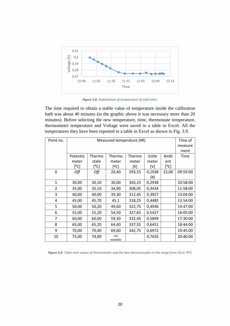
Figure 3.8: Stabilization of temperature of cold wires.

The time required to obtain a stable value of temperature inside the calibration

bath was about 40 minutes (in the graphic above it was necessary more than 20

minutes). Before selecting the new temperature, time, thermostate temperature,

thermometer temperature and Voltage were saved in a table in Excel. All the

temperatures they have been reported in a table in Excel as shown in Fig. 3.9.

Point no. Measured temperature (4R) Time of measure

ment

Potentiometer [⁰C]

Thermostate [⁰C]

Thermometer

[ºC]

Thermometer

[K]

Voltemeter

[V]

Ambient [⁰C]

Time

0 Off Off 20,40 293,55 0,193800

22,00 09:59:00

1 30,00 30,10 30,00 303,15 0,2938 10:58:00

2 35,00 35,10 34,90 308,05 0,3434 11:58:00

3 40,00 40,00 39,30 312,45 0,3927 13:04:00

4 45,00 45,70 45,1 318,25 0,4485 13:54:00

5 50,00 50,20 49,60 322,75 0,4936 14:47:00

6 55,00 55,20 54,50 327,65 0,5427 16:05:00

7 60,00 60,00 59,30 332,45 0,5899 17:30:00

8 65,00 65,20 64,40 337,55 0,6451 18:44:00

9 70,00 70,40 69,60 342,75 0,6972 19:45:00

10 75,00 74,90 not readable

0,7435 20:40:00

Figure 3.9: Table with values of thermometer and the two thermocouples in the range from 20 to 70°C

0,37

0,38

0,39

0,4

0,41

10:48 11:02 11:16 11:31 11:45 12:00 12:14

Vo

ltag

e [V

]

Time

21

3.1.2.3 Results and analysis

The two thermocouples have been calibrated twice since the first results were not

enough accurate. The objective of the calibration is to obtain a relation of the

measured quantity (temperature) with the electrical output expressed in V.

T = m*V + q

(3.8)

It is necessary to obtain a relation as much linear as possible thus obtaining the

slope and the intercept of the line.

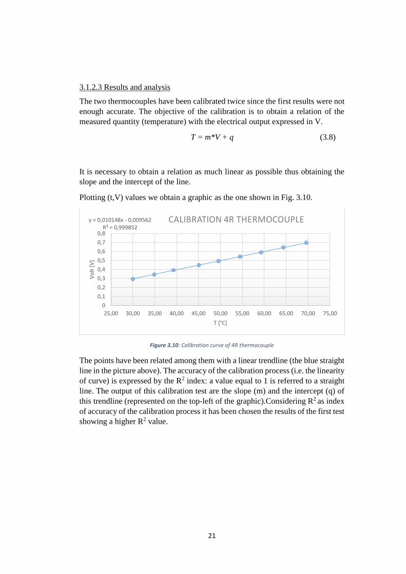
Plotting (t,V) values we obtain a graphic as the one shown in Fig. 3.10.

Figure 3.10: Calibration curve of 4R thermocouple

The points have been related among them with a linear trendline (the blue straight

line in the picture above). The accuracy of the calibration process (i.e. the linearity

of curve) is expressed by the R2 index: a value equal to 1 is referred to a straight

line. The output of this calibration test are the slope (m) and the intercept (q) of

this trendline (represented on the top-left of the graphic).Considering R2 as index

of accuracy of the calibration process it has been chosen the results of the first test

showing a higher R2 value.

y = 0,010148x - 0,009562R² = 0,999852

0

0,1

0,2

0,3

0,4

0,5

0,6

0,7

0,8

25,00 30,00 35,00 40,00 45,00 50,00 55,00 60,00 65,00 70,00 75,00

Vo

lt [

V]

T [°C]

CALIBRATION 4R THERMOCOUPLE

22

T = m*V + q 4R Ttube

Slope (m) 98.5260326 97.787811

Intercept (q) 274.0994312 273.43602

R2 0.999852126 0.9996848

Table 3.2: Results of the calibration of the thermocouples 4R and Ttube

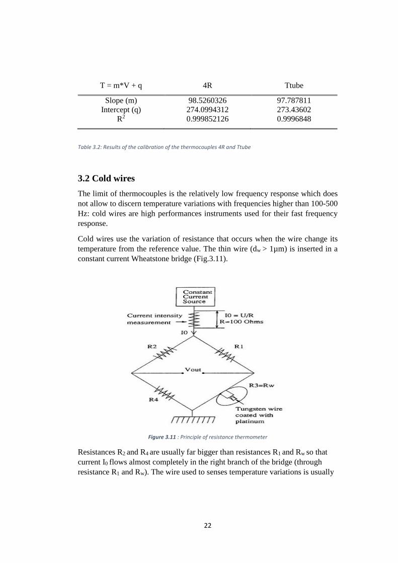
3.2 Cold wires

The limit of thermocouples is the relatively low frequency response which does

not allow to discern temperature variations with frequencies higher than 100-500

Hz: cold wires are high performances instruments used for their fast frequency

response.

Cold wires use the variation of resistance that occurs when the wire change its

temperature from the reference value. The thin wire (dw > 1µm) is inserted in a

constant current Wheatstone bridge (Fig.3.11).

Figure 3.11 : Principle of resistance thermometer

Resistances R2 and R4 are usually far bigger than resistances R1 and Rw so that

current I0 flows almost completely in the right branch of the bridge (through

resistance R1 and Rw). The wire used to senses temperature variations is usually

23

made by tungsten and coated with platinum in order to give a higher mechanical

strength and an appreciable sensitivity to temperature αw. The variation of

resistance with temperature is expressed by:

𝑅𝑤 = 𝑅0[1 + α𝑤(𝑇𝑤 − 𝑇0)]

3.9

𝑅0 =

𝜎0−1𝑙𝑤

𝜋 𝑑𝑤2

4

3.10

where 𝜎0−1 is the resistivity of the wire and lw the length of the wire. The output

supplied by the bridge is a voltage expressed by:

𝑉0 = 𝐼0

𝑅3(𝑅2 + 𝑅4) − 𝑅4(𝑅1 + 𝑅3)

𝑅1 + 𝑅2 + 𝑅3 + 𝑅4= 𝐼0

𝑅3𝑅2 − 𝑅4𝑅1

𝑅1 + 𝑅2 + 𝑅3 + 𝑅4

(3.11)

R3 is the only resistance that changes with temperature, the other having a fixed

value. Considering that ΔR3 = (R3 – R03) is far smaller than the other resistances,

the denominator of the previous formula can be assumed constant and the

electrical output is a linear relation proportional to ΔR3 :

ΔV = Δ𝑅3 𝐼0 G

(3.12)

The bridge must be set in equilibrium(V0=0) changing R2 so that:

𝑅2𝑅03 = 𝑅1𝑅4

(3.13)

The value of current I0 must be enough high to get an appreciable value of ΔV (an

amplifier can be used for this aim). Nevertheless, in order to have a good cold

wire probe, this should be designed to be as much as possible insensitive to gas

velocity: this means that the temperature of the wire must be low and that the

current I0 must be below a certain value in a way to consider Joule effect

24

negligible. The sensitivity of the probe respect to the gas velocity can be computed

starting from a power balance between Joule effect and the power added to the

wire by convective fluxes.

The probe has to register temperature variations occurring with conduction,

convective and radiation phenomena. The physics behind a cold wire can be quite

complicated and some assumptions have to be done in order to get satisfying

results. A brief description of the dynamic model of a cold wire is here reported.

The unsteady behaviour of a cold wire can be described by a first order differential

equation. Indeed the probe, having a certain thermal inertia, needs some time to

respond to a temperature step. As a first approximation, it can be written that the

temperature of the wire depends on its thermal inertia and its capacity to acquire

heat from convective fluxes:

𝑉𝑤𝜌𝑤𝑐𝑤

𝜕𝑇𝑤

𝜕𝑡= −ℎ𝑆𝑤(𝑇𝑤 − 𝑇𝑔)

(3.14)

The equation can be rearranged in an easier way including a time constant τ:

𝜏

𝜕𝑇𝑤

𝜕𝑡+ 𝑇𝑤 = 𝑓(𝑡) = 𝑇𝑔

(3.15)

𝜏 =

𝑉𝑤𝜌𝑤𝑐𝑤

ℎ𝑆𝑤=

𝑑𝑤𝜌𝑤𝑐𝑤

4ℎ

(3.16)

This is a first order differential equation: from signal theory, first order equations

have an analytical formula for transfer function and cut-off frequency. In order to

compute these properties it is necessary to compute the time response constant

which, in turns, requires the knowledge of the convective constant h. This value

comes from Nusselt number expressed as a function of Reynolds number by an

experimental equation:

𝑁𝑢 = 𝐴 + 𝐵 𝑅𝑒𝑛

(3.17)

𝑁𝑢 =

ℎ 𝑑𝑤

𝑘𝑔

(3.18)

25

Where 𝑘𝑔 is the conductivity of the gas. Substituting the equations below in the

formula relative to the time constant we obtain the following equation whose

constants A, B have to be found by experimental tests:

𝜏 =

𝑑𝑤2𝜌𝑤

2 𝑐𝑤

4𝑘𝑔 [𝐴 + 𝐵 (𝜌𝑔𝑣𝑔𝑑𝑤

µ𝑔)

𝑛

]

(3.19)

The cut-off frequency, defined as the frequency at which the modulus of the signal

is attenuated by √2 2⁄ respect to the original value, can be easily found (for first

order equations) as 𝑓𝑐𝑢𝑡−𝑜𝑓𝑓 = 1 2𝜋𝜏⁄ . The results of the cut-off frequency versus

the velocity of gas (𝑣𝑔), taken from Dénos [4], are depicted in Fig. 3.12. It can be

seen that, increasing the gas velocity the convection rises: the probe reacts quicker

(low τ) and the cut-off frequency increases. In the same figure we can see that low

diameter probes have a higher cut-off frequency.

Figure 3.12: The effect of convection (velocity) on the cut-off frequency. A smaller wire has a higher frequency response, which results in a higher cut-off frequency.

In the model described up to now an important phenomenon, source of significant

errors, has not been considered: conduction of heat between wire and prongs. The

wire is mounted between two stain prongs whose dimension are far bigger than

those of the wire (Fig 3.13): conduction cannot be neglected.

26

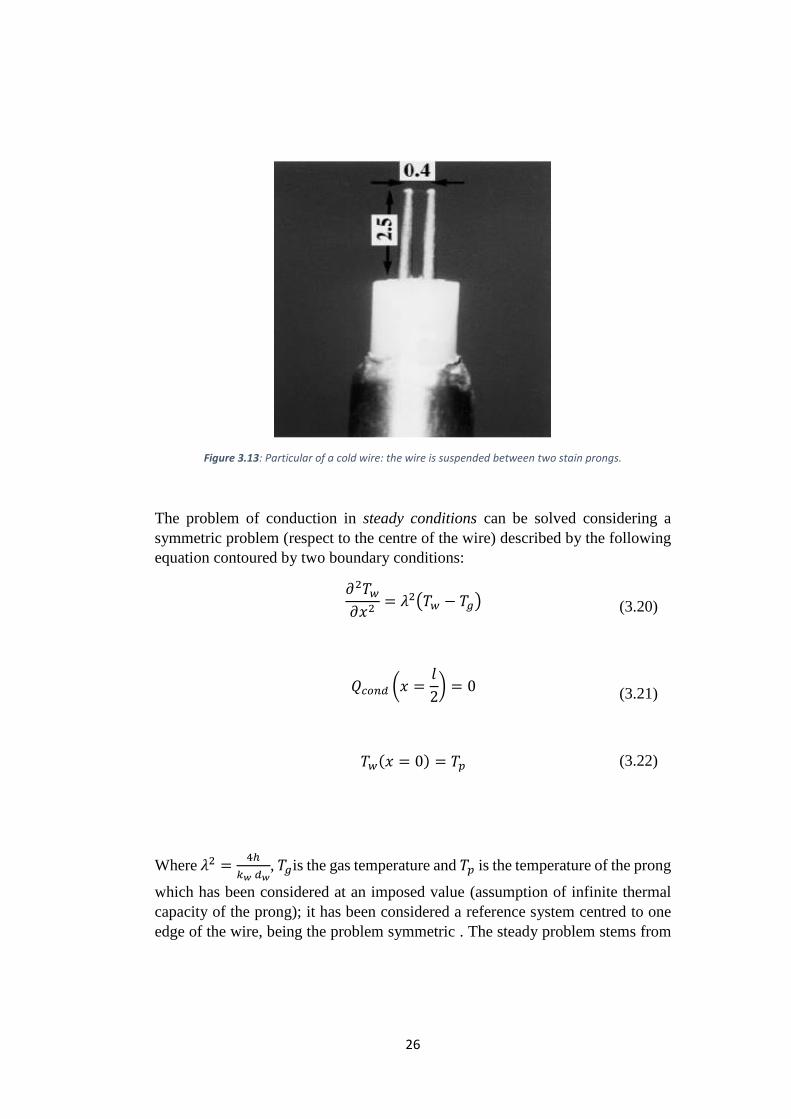
Figure 3.13: Particular of a cold wire: the wire is suspended between two stain prongs.

The problem of conduction in steady conditions can be solved considering a

symmetric problem (respect to the centre of the wire) described by the following

equation contoured by two boundary conditions:

𝜕2𝑇𝑤

𝜕𝑥2= 𝜆2(𝑇𝑤 − 𝑇𝑔)

(3.20)

𝑄𝑐𝑜𝑛𝑑 (𝑥 =

𝑙

2) = 0

(3.21)

𝑇𝑤(𝑥 = 0) = 𝑇𝑝

(3.22)

Where 𝜆2 =4ℎ

𝑘𝑤 𝑑𝑤, 𝑇𝑔is the gas temperature and 𝑇𝑝 is the temperature of the prong

which has been considered at an imposed value (assumption of infinite thermal

capacity of the prong); it has been considered a reference system centred to one

edge of the wire, being the problem symmetric . The steady problem stems from

27

a heat balance between conductive and convective fluxes (unsteady phenomena

and Joule effects have been neglected). The results of this equation computed by

Dénos are reported in Fig. 3.14. It has been defined the ratio 𝑇𝑤−𝑇𝑝

𝑇𝑎−𝑇𝑝 , being 𝑇𝑎the

temperature of the gas and 𝑇𝑝the temperature of the prong: this is an index of the

disturbance of conduction phenomena between wire and prong. When this ratio

is equal to 1 there is no interference between wire and prong and the wire has (at

least theoretically) the same temperature of the gas. The parameter 𝑙 𝑑⁄ , length

over diameter of the wire, is a non-dimensional number describing its geometry.

A high 𝑙 𝑑⁄ value refers to a thin wire developing in length.

Figure 3.14: The effect of conduction of the prongs: the temperature of the wire is closer to the temperature of the gas in the centre of the wire (less conduction effect); the conduction error decreases considering wire with a high l/d ratio. Velocity has an important dependence on the mean wire temperature: higher velocity are associated to higher convection and a reduced conduction error.

It can be noticed that conduction effects are smaller when we refer to the

temperature at the centre of the wire (𝑥 𝑙 = 0.5)⁄ . When l/d rises, the conduction

errors affect only the edges of the wire. The figure on the right (always referring

to Fig 3.14) shows the favourable effects of a higher gas velocity: higher

convection (h, coming from a higher gas velocity) reduces the conduction effects

between wire and prongs and the mean temperature of the wire approaches the

temperature of the gas.

The description of unsteady conduction between wire and prongs requires a more

complicated physical description. Referring always to [4] only a short resume will

28

be given. The unsteady conduction phenomena is described by the following

differential equation contoured by boundary conditions (temperature of the

prongs) and initial conditions:

𝜕𝑇𝑤

𝜕𝑡= 𝛼

𝜕2𝑇𝑤

𝜕𝑥2−

1

𝜏(𝑇𝑤 − 𝑇𝑔)

(3.23)

Where =𝑘𝑤

𝜌𝑤𝑐𝑤 , 𝜏 =

𝑑𝑤𝜌𝑤𝑐𝑤

4ℎ . This equation can be solved using as numerical

solution the implicit Crank-Nicholson scheme. The equation have been

discretized in the time and space domain obtaining the following equation:

𝑇𝑖𝑛+1−𝑇𝑖

𝑛

𝛥𝑇=

𝛼[𝜂(𝑇𝑖+1

𝑛+1−2𝑇𝑖𝑛+1+𝑇𝑖−1

𝑛+1)+(1−𝜂)(𝑇𝑖+1𝑛−2𝑇𝑖

𝑛+𝑇𝑖−1𝑛)]

𝛥𝑥2 −1

𝜏[(𝜂𝑇𝑖

𝑛+1 + (1 − 𝜂)𝑇𝑖𝑛) − 𝑇𝑔

𝑛]

(3.23.1)

The numerical system has been tested with an input signal. A sine wave signal of

gas temperature has been used as input for a prong-wire system in order to test its

response. This sine signal has been tested at different frequencies (100Hz,

1000Hz) and several values of gain have been obtained. These results are shown

in Fig 3.15. It can be noticed that, at low frequency, both prong and wire follow

the sine input because the gain is 0 dB; at higher frequencies the prong is not able

to follow the input signal. In the picture representing the transfer function we can

observe a plateau region. At further higher frequencies neither the tungsten wire

can reproduce the gas temperature signal: the gain decreases abruptly. Other

results relative to the influence of the prong time constant on the frequency

response can be found in the paper written by Dénos [4].

29

Figure 3.15: (left) Transfer function of the wire-prong system: it is possible to see the effects of velocity. (right): The numerical system represented in equation 3.23.1 has been tested with a sinusoidal input for different frequencies. The prong is not able to follow the input at high frequency.

Another resolution for the unsteady conduction problem can be found considering

the first order system as a discrete system described by the following equation:

𝑇𝑤𝑛+1 − 𝑇𝑤

𝑛

𝛥𝑡= −

1

𝜏(𝑇𝑤

𝑛 − 𝑇𝑔𝑛)

(3.24)

Better results can be achieved considering combinations of discrete first order

systems. The probe output (T) can be written as a linear combination of the

responses of wire and prongs: this will discussed in detail in chapter 4 and chapter

5.

3.2.1 Cold wire static calibration (oven)

The cold wires have been calibrated with static tests: they have been tested in

steady conditions, i.e. neglecting dynamic effects, using the oven and the heated

jet.

The static calibration in the oven and heated jet has been done for two cold wires:

DAO121A (identified with letter B) and DAO123A (identified with letter A). The

two probes are represented in Fig 3.16.

Each probe has two transducers: the first one placed in the middle and indicated

with number 2; the second one placed at the edge and indicated with number 1.

30

The wire is made of tungsten and has a length (lw) of 1 mm and a diameter (dw) of

2.5µm; it is held by two prongs 2 mm long.

Figure 3.16: Cold wires DAO121A, DAO123A

3.2.1.1 Calibration Process

The calibration in still air has been done in steady conditions: the cold wire and a

thermocouple have been placed inside a metallic box which, in turn, have been

put inside an oven (Fig. 3.17(a), Fig.17(b)). The electric cables of the probes come

out of the oven through a hole which have been closed with red plasticine in order

not to have heat dispersion (see Fig. 3.17(c) ).

DAO121A has been tested with 4R thermocouple; DAO123A has been tested

with 2R thermocouple. The thermocouples have been linked to an amplifier in

order to obtain significant values as output (in detail: thermocouple 4R was linked

with TC amplifier TU4, thermocouple 2R was linked with TC amplifier TU7).

For the calibration of these probes two cold wire boxes have been used: the black

one (TUCW3) and the white one (TUCW2). These boxes basically consist in a

Wheatstone bridge in which one of the four resistances is the cold wire, linked to

the box by its input entries (Fig. 3.18).

31

Figure 3.17: Setup for the static calibration in the oven

32

Figure 3.18: (a) Schematic representation of the wiring of a cold wire; (b) power supplier.

The cold wire box is linked to a power supply (Fig. 3.18 (b)) which produces the

desired value of voltage: for this test it has been set a value of ± 15V in order

obtain a current inside the wire of around 0.2 mA. It’s important to have an electric

current of small intensity in order to have a negligible Joule Effect. Through some

BNC cables it was possible to read the output of the box (voltage of the bridge

and current inside the wire) displayed in a multimeter.

For the calibration of the cold wire it has been chosen to set the range of

temperatures between 20 and 90 °C with a ΔT of 10°C between two points. Before

starting the test, the stability of the electronic setup has been tested monitoring

the values of the cold wire and current outputs in function of time at ambient

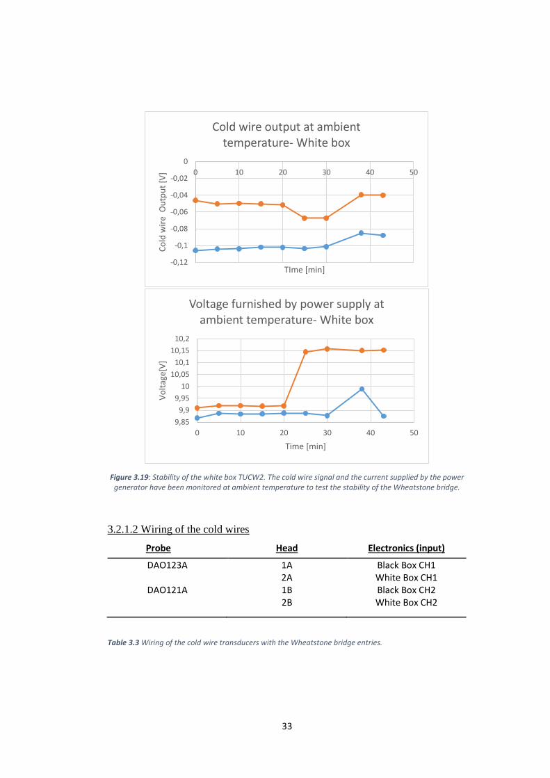
temperature. This is shown in Fig. 3.19: these data are relative to the white box

TUCW2 and it can be noticed that they drift a bit.

Once the data relative to the current, cold wire and thermocouples outputs have

been taken at ambient temperature, the oven is heated up to the prefixed target

temperature. To obtain a stable value it took 1h40 minutes. The data have been

registered up to 90°C degrees and the calibration was brought to an end in two

days. As done for the calibration of thermocouples, also for the cold wires these

data have been related with a linear trendline: using Excel it was possible to obtain

the slope, the intercept and the R2 of the curve.

33

Figure 3.19: Stability of the white box TUCW2. The cold wire signal and the current supplied by the power generator have been monitored at ambient temperature to test the stability of the Wheatstone bridge.

3.2.1.2 Wiring of the cold wires

Probe Head Electronics (input)

DAO123A 1A Black Box CH1 2A White Box CH1

DAO121A 1B Black Box CH2 2B White Box CH2

Table 3.3 Wiring of the cold wire transducers with the Wheatstone bridge entries.

-0,12

-0,1

-0,08

-0,06

-0,04

-0,02

0

0 10 20 30 40 50

Co

ld w

ire

Ou

tpu

t [V

]

TIme [min]

Cold wire output at ambient temperature- White box

9,85

9,9

9,95

10

10,05

10,1

10,15

10,2

0 10 20 30 40 50

Vo

ltag

e[V

]

Time [min]

Voltage furnished by power supply at ambient temperature- White box

34

3.2.1.3 Results

The following graphics (Fig. 3.20) are the calibration curves for the two probes.

Figure 3.20: Results of the static calibration in the oven of the two cold wires DAO121A , DAO123A

y = -0,05593x + 0,94313R² = 0,99931

y = -0,09847884x + 1,87795631R² = 0,99997421

-8

-7

-6

-5

-4

-3

-2

-1

0

0 20 40 60 80 100

Co

ld w

ire

ou

tpu

t [V

}

Temperature [°C]

TUCW2 (White Box) , 20-90 °C 2A 2B

y = 0,03341x - 0,71082R² = 0,99923

y = 0,0308x - 0,7998R² = 0,9996

-0,5

0

0,5

1

1,5

2

2,5

0 20 40 60 80 100

Co

ld w

ire

ou

tpu

t [V

]

Temperature [°C]

TUCW3 (Black Box), 20-90 °C 1A 1B

35

3.2.2 Cold wire static calibration (heated jet)

The calibration in heated jet has been done using a more complicated setup. The

cold wire has been tested always in static conditions registering its outputs at

different Mach and temperature of an air jet.

For these tests the cold wire has been mounted on variable height support in order

to put manually the probe inside and outside the heated jet setting the height of

the support (Fig. 3.21). This support has been placed near a facility that blows the

jet of air through a nozzle: changing the height of the support the head of the

transducer was submerged into the flow. The facility for the heated jet was linked

with a pipe to a heating system that, in turn, was linked to the air pressurised

reservoir of the Von Karman Institute. The head of the probe was tested only for

few seconds into the flow to preserve the wire which is extremely fragile: after

having taken the data the support was moved manually to remove the probe from

the jet.

The test consisted in measuring the output of the cold wire when inserted into a

flow with known temperature and Mach conditions. At the same time pressure

and temperature variations were registered with other probes. Before starting the

test, the pressurized air reservoir was opened to reach a sufficient ΔP to get the

desired Mach number.

Figure 3.21: Experimental setup for the static calibration of the cold wire in the jet; it is visible the metallic support used to set the position of the cold wire.

36

3.2.2.1 Experimental Setup

The cold wires have been linked to the Wheatstone bridge as done in the

calibration in the oven: the tested transducer has been linked to the input of the

box used as Wheatstone bridge (Fig. 3.22); this box, in turn, has been connected

to a power supply and to a multimeter in order to read the output of the probe.

The pressurized air has been blown through a nozzle. Inside the nozzle it has been

placed a differential pressure transducer (SENSYM) and a thermocouple (2R):

the latter has been linked to an amplifier in order to obtain significant values.

Outside the nozzle, through some rigid supports it has been installed the second

thermocouple (4R, connected to an amplifier) while the cold wire has been

mounted on a variable height support, as mentioned before.

The connections of the heads of the probes with the Wheatstone bridge

(black/white boxes) are the same used for the calibration in the oven.

Figure 3.22: The cold wire boxes (Wheatstone bridge)

37

3.2.2.2 Pressure Readings

A differential pressure transducer (SENSYM, R4S4) has been inserted inside the

nozzle in a way to get differential pressure readings. Before using the probe in the

static test the transducer has been calibrated: one head of the probe has been

connected inside the sealed case of the pressure calibrator through a thin plastic

pipe while the other was kept to ambient pressure (Fig. 3.23). The transducer has

been linked with a power supply through a connector: through a multimeter it was

possible to read the electrical output of the probe.

Figure 3.23: Setup for the calibration of the SENSYM (differential pressure transducer)

The pressure calibrator output was set initially to zero. Once the sealed chamber

was closed it was possible to add or subtract pressure to one side of the transducer

(the other side being at constant ambient pressure) with the handles of the

instrument. As done for the calibration of thermocouples also in this case several

points of pressure-voltage have been taken and have been inserted in Excel in

order to get a linear trend with values of slope and intercept. As can be seen in the

following graphic this instrument has a high R2 (>0.99999).

38

Figure 3.24: Calibration curve of the SENSYM R4S4

3.2.2.3 Temperature Readings

Two temperature probes have been installed in the facility to get more details on

the evolution of temperature. The 2R thermocouple was mounted inside the

nozzle and linked to the TC amplifier TU7; the 4R thermocouple was mounted

with a rigid support right at the exit of the nozzle and linked to the TC amplifier

TU4. In Fig. 3.25 we can see that the head of the thermocouple 4R is closely

placed near one of the two heads of the cold wire.

Other two thermocouples have been installed inside the heating system (Fig.

3.26).

Figure 3.25: Thermocouple 4R (up) and cold wire (put horizontally).

y = 3,34675550x - 0,37742555R² = 0,99999870

0,0000

1,0000

2,0000

3,0000

4,0000

5,0000

0,8000 0,9000 1,0000 1,1000 1,2000 1,3000

Vo

ltag

e [

V]

P [bar]

Calibration of the SENSYM

39

Figure 3.26: The heating system for the air pressurized reservoir. It is provided with two thermocouples to monitor the temperature before the air reach the nozzle.

3.2.2.4 Setting Mach number

The tests in the heated jet have been done using several Mach numbers. The

desired value has been reached using air pressurized into a reservoir.

The data of ambient pressure came from the server of Von Karman Institute.

Knowing the value of Mach number required for the test and the ambient pressure

it was possible to obtain the required total pressure using equation (3.25)

𝑃𝑡𝑜𝑡

𝑃𝑠= [1 + (

𝛾 − 1

2) 𝑀2]

𝛾𝛾−1

(3.25)

Being 𝑃𝑠 the ambient pressure and 𝑘 the specific heat ratio of air. The air has been

considered a perfect gas, having 𝛾 = 1.4, specific heat at constant pressure 𝐶𝑝 =

1.005𝐾𝐽

𝐾𝑔 𝐾 and specific constant 𝑅 = 287.05

𝐽 𝐾𝑔

𝐾 .

The dynamic pressure dP stems from the difference from the total and static

pressure (𝑃𝑎𝑚𝑏) :

𝑑𝑃 = 𝑃𝑡𝑜𝑡 − 𝑃𝑎𝑚𝑏

(3.26)

40

The related value expressed in Volts in the multimeter is obtained using the values

obtained with the calibration of the SENSYM (see Pressure Readings).

3.2.2.5 Setting temperature of the air

As mentioned before, the air coming from the pressurized reservoir has been

heated up to a desired temperature. To obtain the required value air passed into

the heat exchanger shown in Fig. 3.26. The temperature has been chosen using a

handle while the rate of heating has been changed increasing the current inside

the resistances in the heat exchanger thus increasing Joule effect.

3.2.2.6 Calibration Process

The two probes DAO121A and DAO123A have been calibrated in the heated jet:

in each experiment the head of the transducer was tested at different Mach

numbers and different temperatures. The values of Mach have been chosen at

0.05, 0.2 and 0.3; for each velocity (Mach number) the probe was tested at 10

different temperatures (from 20°C to 65-70°C).

The electronics of the bridge have been set up in order to get small current in the

wire (values lower than 2mA); as done for the calibration in the oven the power

supply was arranged to give 15V of voltage.

The first point of calibration curve has been taken at ambient temperature at Mach

0. After having opened the valve of the air pressurized reservoir and having

chosen the correct value of total pressure to apply it was possible to start the

calibration.

The first test has been done at Mach 0.05 and ambient temperature (~17°C). For

each point the data of the two thermocouples, the cold wire and the pressure

transducer have been monitored. The cold wire has been exposed to the air flux

for few seconds in order to preserve it. After having taken the data, the

temperature was raised to the target temperature using the handle of the heat

exchanger.

The same procedure has been followed raising the Mach number to 0.2 and 0.3:

before starting the calibration to a new Mach number starting from ambient

temperature we had to wait for a while since the heat exchanger was still hot.

41

3.2.2.7 Results

During the investigations the head 2A (DAO123A) got broken when tested at

Mach 0.3: the wire was repaired and tested again. The results obtained with the

two wires (of head 2A) have been compared and discussed at the end of the

paragraph. In the following graphs it have been shown the results of the output of

the cold wire in function of the temperature inside the nozzle (temperature

registered by the thermocouple 2R) and temperature in the jet (temperature

registered by the thermocouple 4R). The subscript 1 refers to the CW-TC Jet

Temp; the subscript 2 refers to the CW-Nozzle temp.

DAO123A- Head 1A

In this graphic are visible the effects of Reynolds causing the curve to change

slope and intercept with the Mach number. The results relative to the calibration

coefficients are reported in table 3.4. The electric output of the cold wire has

been associated to the value of temperature registered by the thermocouple

placed near the cold wire in the jet.

42

DAO123A- Head 2A

The probe got broken testing it at 70°C. It has been repaired and tested again

.

Mach 0.3 (second calibration, after reparation)

After the reparation the calibration curve of head 2A has changed: there’s a

small change in the slope of the curves (before and after reparation) of 3.34%

but a significant change of the intercept that can be due to the variation of the

overall resistances. The two curves are shown in the following picture. The

head 1A which has been tested twice even if it hasn’t been repaired keeps the

same values of intercept and slope with insignificant variations.

y2 = -0,039324x + 0,951801R² = 0,999685

y1 = -0,043300x + 0,997025R² = 0,999394

-2

-1,5

-1

-0,5

0

0,5

0,0 10,0 20,0 30,0 40,0 50,0 60,0 70,0

Vo

ltag

e [

V]

Temperature [°C]

CW - Nozzle Temp CW - TC Jet Temp

Lineare (CW - Nozzle Temp) Lineare (CW - TC Jet Temp)

43

Figure 3.27: Comparison of head 2A before and after reparation. There is significant variation in the intercept due to the change of the overall resistance of the cold wire.

3.2.2.7.3 DAO123A- Head 1B

Mach 0.3

y2 = -0,039324x + 0,951801R² = 0,999685

y1 = -0,040683x + 0,572120R² = 0,999967

-3

-2

-1

0

1

0,0 10,0 20,0 30,0 40,0 50,0 60,0 70,0

Vo

ltag

e [

V]

Temperature [°C]

Head 2A (repaired) Head 2A

Lineare (Head 2A (repaired)) Lineare (Head 2A)

y2 = 0,020896x - 0,666775R² = 0,999929

y1 = 0,021459x - 0,669667R² = 0,999873

-0,2

0

0,2

0,4

0,6

0,8

1

0,0 10,0 20,0 30,0 40,0 50,0 60,0 70,0 80,0

Vo

ltag

e [

V]

Temperature [°C]

CW - Nozzle Temp CW - TC Jet Temp

Lineare (CW - Nozzle Temp) Lineare (CW - TC Jet Temp)

44

3.2.2.7.4 DAO123A- Head 2B

Mach 0.3

The probe DAO123A Head-2A has been tested at different Mach numbers: the

slope changes without following a precise relation with the velocity. Changes of

the slope are in the order of 5% and can be related to Reynolds effects.

Probe Head Mach Reynolds

TTOT= 323 K

a b R2

T = a*V + b (with T in °C)

DAO123A 1A 0 - 29,92972 21,2746 0,999232

0.05 2.49 43,16862 25,0399 0,999810

0.2 10.04 41,66523 26,8696 0,999227

0.3 15.25 43,58036 19,1749 0,999737

2A 0 - -17,8797 16,8628 0,999312

0.3 15.25 -25,4295 24,2039 0,999685

DAO121A 1B 0 - 32,44697 25,95118 0,99955

0.3 15.25 47,85493 31,90849 0,99993

2B 0 - -10,15446 19,06964 0,99997

0.3 15.25 -14,25648 17,56851 0,99957

Table 3.4: Results of the static calibration of cold wire

y2 = -0,070144x + 1,232318R² = 0,999565

y1 = -0,070734x + 1,186807R² = 0,996459

-4,0

-3,0

-2,0

-1,0

0,0

0,0 10,0 20,0 30,0 40,0 50,0 60,0 70,0 80,0

CW - Nozzle Temp CW - TC Jet Temp

Lineare (CW - Nozzle Temp) Lineare (CW - TC Jet Temp)

45

Chapter 4

Numerical Filtering and Signal

Compensation

The calibration process has been done in order to obtain a relation between the

electrical output of the probes and the desired physical characteristic (i.e.

temperature, pressure). The modern transducers have a high sensitivity to physical

variations and it is possible to display these changes in digital multimeteres

obtaining high accuracy measurements.

The main problem of electrical instruments is that they produce an internal noise

associated with an unsteady distribution of electrical charge inside the instrument

itself. This is known as thermal noise: the microscopic variations inside a

conductive material turn into macroscopic variations (fluctuations) of the output

(Voltage). This kind of fluctuations, described with probabilistic tools, depends

on the material properties and is not possible to eliminate them: they superimpose

on the original signal causing an alteration or distortion of the signal itself.

For this reason it becomes important to adopt some tools in order to obtain

experimental results that can be easily interpreted: the signal is filtered and

cleaned from unnecessary noise and disturbances. In this chapter will be

described the numerical analysis done in order to obtain the amplitude and phase

curves of analogue filters used for experiments in CT3.

On the other hand, this chapter deals with the problem of the theory on numerical

compensation of signals. Transducer have physical limits that do not allow to get

accurate results when the registered phenomena are extremely fast. The

compensation allows reconstructing the real signal starting from the original one

through the probe transfer function. It is possible to obtain it through experimental

tests and compensate the signal through the inverse of the transfer function. This

problem will be described in detail in the second part of this chapter; the

experimental activity is presented in the last chapter.

46

4.1 Numerical filtering

In this paragraph it is shown the description of the experimental tests done in order

to characterize the filter boxes and a quick description of the code developed on

Matlab to process the obtained data.

4.1.1 Experimental Setup

4.1.1.1 Filter boxes

The filter boxes utilised for the experiments are those ones shown in Fig. 4.1. The

one on the left, the bigger one, has 4 boards that, in turn, have 4 channels each. In

every channel there are 4 entries relative to the Input, Raw Output, Low Pass

Output, High Pass Output. Each channel is done in such a way that the Raw

Output reproduces exactly the input signal while the Low Pass Output filters the

input frequencies higher than 100 Hz and the High Pass Output filters those ones

lower than 750 Hz. Before starting the data acquisition the electronic cards that

powered the filter box have been set up as shown in Fig. 4.2.

Figure 4.1: Filter boxes: each channel has a certain behaviour in the frequency domain. The aim of testing these boxes is getting the Bode diagrams of every channel.

The filter box shown in Fig. 4.1 on the right has 2 boards with 4 channel each,

which, in turn have the same four entries: Input, Raw Output, Low Pass Output,

High Pass Output (same Low Pass, High pass frequencies as the first filter box).

Channel 1 and channel 3 of the second board are not working.

47

Figure 4.2: Electronic cards. The filter boxes are supplied by electronic cards.

4.1.1.2 Frequency generator

The signal to be tested in the filter boxes has been generated by the frequency

generator depicted in Fig. 4.3. With this instrument it is possible to generate

electric input signals at the desired frequency and shape (triangular, sinusoidal,

step-shaped). The frequency generator has been linked with a cable to the input

entry of the chosen board-channel of the filter box. It has been decided to analyse

a sinusoidal input signal of 0.7 0-to-peak amplitude (1.4 peak-to-peak amplitude)

in a particular range of frequencies (0-200000 Hz, more detail later in the

paragraph 4.1.1.4).

48

Figure 4.3: The frequency generator is used to produce signal of known shape and frequency

4.1.1.3 Data acquisition system

The three output entries (Raw, Low-Pass, High-Pass) have been linked to

GENESIS, a data acquisition system (DAS). This machine is used to acquire

electric data at a high sampling rate from a continuous input signal. The three

outputs of the filter have been linked to 3 of the 8 channels of a port (GENESIS

has 8 ports). In Fig. 4.4 a representation of GENESIS. For the tests it has been

chosen a sampling frequency of 1MHz. A computer interacts with the DAS

through Perception, a software that allows to set some configurations of the data

acquisition system and register easily the data in different formats. Having chosen

the amplitude of the input signal equal to 0.7V, it has been set to 5V the span

range for the Input, Raw Output, Low Pass Output and to 20V for the High Pass

Output.

In the end of the paragraph it’s sketched the whole setup used for this test (Fig.

4.5).

49

Figure 4.4: GENESIS data acquisition system. It has 8 ports, each provided with 8 channels

4.1.1.4 Analysed frequencies

According to Nyquist theorem, the sampling frequency must be higher than twice

the maximum frequency of the analysed signal. Having set the sampling

frequency to 1MHz the range of the possible frequencies analysable is 0-

500000Hz. For these test was sufficient to test the filter box in a range 5-

200000Hz, along 20 points. The frequencies range to be analysed was chosen to

be equi-spaced in the logarithmic scale. Being L=5 the lowest frequency,

U=200000 the highest one and n = 20 the number of frequencies, it was found the

factor k used to find all the equi-spaced frequencies in the logarithmic scale:

𝑘 = (𝑈

𝐿)

11−𝑛

(4.1)

𝑓(𝑛) = 𝑓(𝑛 − 1) ∗ 𝑘

(4.2)

In this list of frequencies were added also values at 100 Hz, 600Hz, 900 (the cut-

off frequencies of the filters) and the value at 0 Hz (actually in the test it has been

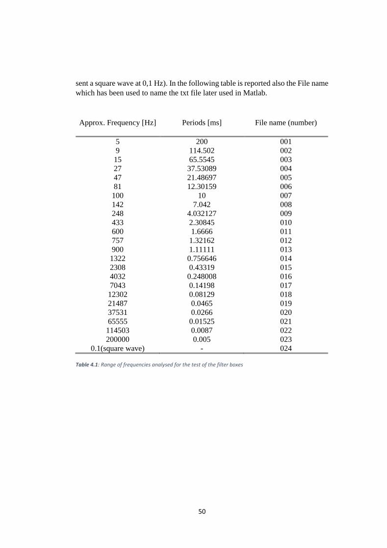
50

sent a square wave at 0,1 Hz). In the following table is reported also the File name

which has been used to name the txt file later used in Matlab.

Approx. Frequency [Hz] Periods [ms] File name (number)

5 200 001

9 114.502 002

15 65.5545 003

27 37.53089 004

47 21.48697 005

81 12.30159 006

100 10 007

142 7.042 008

248 4.032127 009

433 2.30845 010

600 1.6666 011

757 1.32162 012

900 1.11111 013

1322 0.756646 014

2308 0.43319 015

4032 0.248008 016

7043 0.14198 017

12302 0.08129 018

21487 0.0465 019

37531 0.0266 020

65555 0.01525 021

114503 0.0087 022

200000 0.005 023

0.1(square wave) - 024 Table 4.1: Range of frequencies analysed for the test of the filter boxes

51

Figure 4.5: Experimental setup for filter boxes tests.

4.1.2 Experimental Procedure to test Filter Box

Once the experimental setup was settled it was possible to test the known input

signals in the filter box. The frequency generator was set to the desired

shape/frequency; the input and outputs responses of the filter box were displayed

in Perception. Using a trigger it was possible to acquire data with the required

options chosen in the software.

The data have been registered as .txt files like the one showed in the following

image (Fig 4.6). The first column shows the vector of times; the other columns

show respectively the values of the Input, Raw, Low-Pass and High-Pass outputs

in each sampling instant. Each columns has one million points.

52

Figure 4.6: The output of the acquisition obtained with Perception. The first columns is the sampling time; the other 4 columns are referred to the channels of the filter box

Each channel was tested for all the 24 frequencies (see Table 4.1); the same work

was done for all the channels of both filter boxes. Each .txt file was named in the

formula B(number)CH(number) number (example B1CH1001) in order to be read

by the automatized Matlab code.

4.1.3 Post-processing of data

The aim of this test was to understand the behaviour of the analogue filters using

some known inputs. Basically, for each frequency, the input signal was compared

to the output and it was defined the Gain and the Phase at that frequency. The

Gain is defined as the ratio of the amplitude of the output over the amplitude of

the input 𝐴𝑜𝑢𝑡 𝐴𝑖𝑛⁄ ; it’s quite common to express the Gain in dB and then plot the

results on a logarithmic scale using this formula:

𝐺(𝑑𝐵) = 20𝑙𝑜𝑔 (

𝐴𝑜𝑢𝑡

𝐴𝑖𝑛)

(4.3)

The phase shift is defined as the delay of the output signal respect to the input

one. It is usually expressed in seconds [s] or radians. It is possible to convert the

unit using the following formula:

53

1 [rad] =

𝑇

2𝜋[s]

(4.4)

Being T the period of the signal. It is not complicated to find the gain and the

phase shift of an analogue signal (for example a sinus): facing this problem with

digital signals, as in our case, is much more complicate especially if this process

has to be done in an automatized routine for generic input signals. In Fig. 4.7 is

possible to see a digitalised sinusoidal signal. It is a vector of 1 million points: it

looks like a normal analogue signal at first sight; but it’s a signal affected by a

certain level of noise as can be seen zooming on the image.

Figure 4.7: The acquired sinusoidal signal is affected by noise that has to be dealt correctle.

For this reason it’s necessary to write a code which is able to detect the absolute

peaks in the signal or find the zero values in the time vector. In the next paragraphs

are quickly shown two processes used to compute frequency, gain and phase shift

of the signals.

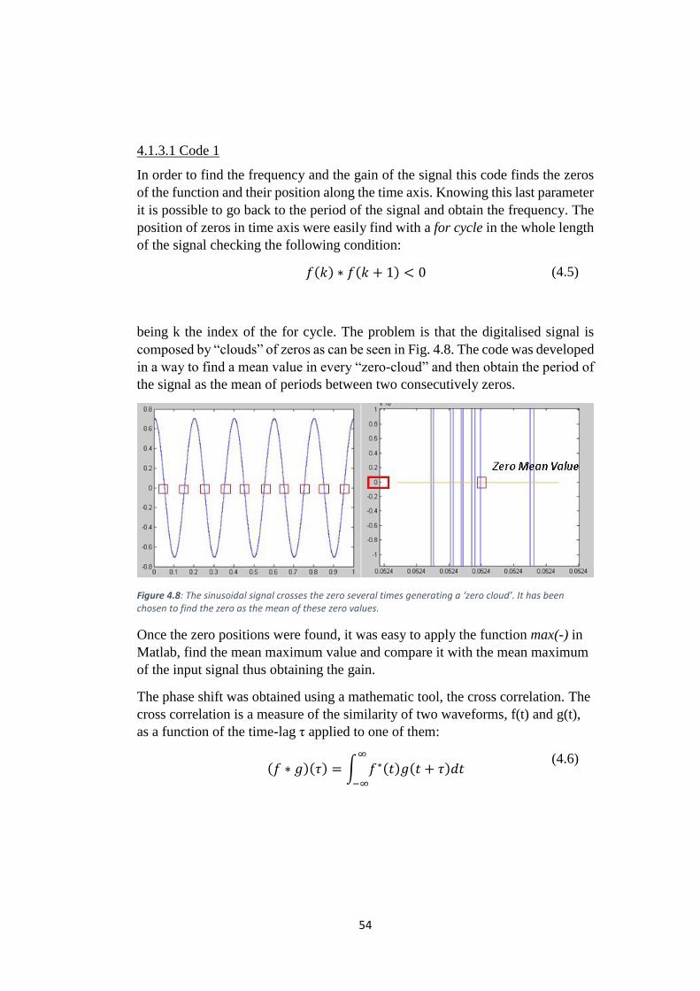
54

4.1.3.1 Code 1

In order to find the frequency and the gain of the signal this code finds the zeros

of the function and their position along the time axis. Knowing this last parameter

it is possible to go back to the period of the signal and obtain the frequency. The

position of zeros in time axis were easily find with a for cycle in the whole length

of the signal checking the following condition:

𝑓(𝑘) ∗ 𝑓(𝑘 + 1) < 0

(4.5)

being k the index of the for cycle. The problem is that the digitalised signal is

composed by “clouds” of zeros as can be seen in Fig. 4.8. The code was developed

in a way to find a mean value in every “zero-cloud” and then obtain the period of

the signal as the mean of periods between two consecutively zeros.

Figure 4.8: The sinusoidal signal crosses the zero several times generating a ‘zero cloud’. It has been chosen to find the zero as the mean of these zero values.

Once the zero positions were found, it was easy to apply the function max(-) in

Matlab, find the mean maximum value and compare it with the mean maximum

of the input signal thus obtaining the gain.

The phase shift was obtained using a mathematic tool, the cross correlation. The

cross correlation is a measure of the similarity of two waveforms, f(t) and g(t),

as a function of the time-lag τ applied to one of them:

(𝑓 ∗ 𝑔)(𝜏) = ∫ 𝑓∗(𝑡)𝑔(𝑡 + 𝜏)𝑑𝑡

∞

−∞

(4.6)

55

where f* denotes the complex conjugate of f. In the code they were used the

input and output vectors of the signal.

[r,lags] = xcorr(Input_s,Output_s);

(4.7)

The bigger is the value (𝑓 ∗ 𝑔)(𝜏), r in the code, the more similar are the two

functions. The biggest value of (𝑓 ∗ 𝑔)(𝜏), r(k), it’s obtained when the two

signals overlap. The phase shift between the two signal is obtained in this

condition: this is equal to τ (or lags(k)in Matlab ). In Fig. 4.9 an example of

the cross-correlation between two signals.

Figure 4.9: An example of cross-correlation

The code was working correctly for frequencies up to 65000 Hz. It was not

possible to obtain frequency, gain and phase shift for the last two frequencies

114000 and 200000Hz because of the high computational cost.

56

4.1.3.2 Code 2

To get the results for all the frequencies the code was re-written using some other

tools to simplify the computations. Before starting any computation the signal was

filtered from the noise using the function ‘smooth’ in Matlab. The following

picture shows how the signal appears after this filtering:

Figure 4.10: The signal before and after having used the ‘smooth’ function in Matlab

The frequency was computed easily using the Fourier Fast Transform on the

signal: the frequency was founds as the maximum of the modulus of this vector.

The results of an FFT is shown in Fig. 4.11.

The Gain was easily computed using a function in Matlab called ‘peakdet’: it is

possible to obtain the maxima and their positions in the input vector simply setting

the input vector and a threshold value between two peaks as input of the function.

Once obtained the value of the peaks, it was done the mean among them and this

value was divided by the mean value of the peaks of the input signal.

Figure 4.11: The Fast Fourier Transfrom of a signal allows to find the frequency content of a signal.

57

The phase shift was computed “manually” subtracting the position values of

maxima for the output and input signals and then taking a mean value. This

second code was preferred to the other, having a lower computational cost and

thus allowing to test the filter box at high frequencies ( >100000Hz). In the next

paragraph it will be shown the results obtained testing the two filter boxes with

this code.

4.1.4 Results

Each channel was tested using this code and it took 15 minutes to compute gain,

frequency and phase shift for all the selected range of frequencies (0-200000Hz).

This code was preferred respect to the first one because faster and it allowed to

compute the behaviour of the box also at high frequencies. The results have been

grouped in different graphics: in the following pictures the channels will be

indicated by the abbreviation F-B-C which stands for filter, board, channel

followed by the number.

58

GAIN: High-Pass channel

Figure 4.12

Figure 4.13

59

GAIN: Low-Pass channel

Figure 4.14

Figure 4.15

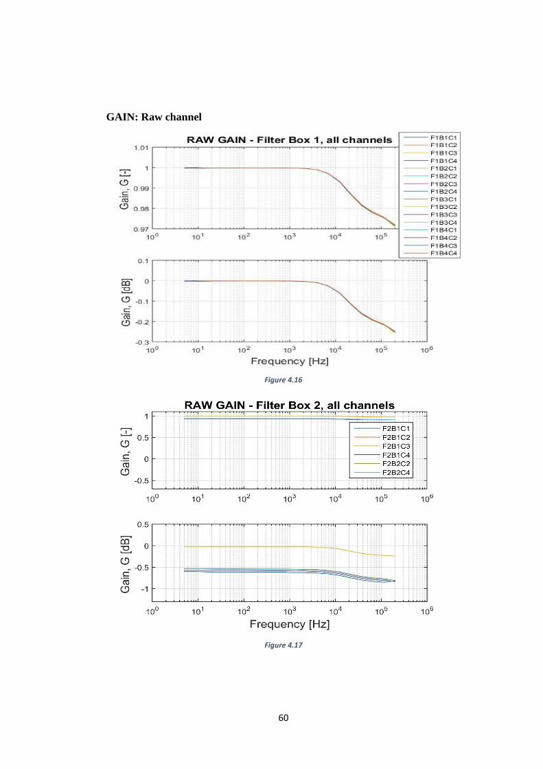
60

GAIN: Raw channel

Figure 4.16

Figure 4.17

61

In these graphics is represented the gain (absolute and expressed in decibel) of all

the channels belonging to the filter box 1 and filter box 2. It can be noticed that,

as expected, the high-pass filter (shown in figures 4.12 and 4.13) has a cut-off

frequency of 100 Hz as indicated in the box. The gain in the band-pass region is

20dB as was set in the electronic card: the signal is amplified by a factor 10 for

frequencies between 100Hz and 12000Hz. Starting from 10000Hz the signal

amplitude is attenuated since the filter box is equipped by an internal anti-aliasing

filter. Looking the graphics in the bottom, those whose gain is expressed in

decibel we can observe that the filter box behaves like a second-order filter: the

gain increases by 40 decibel each decade.

The Low-Pass gain is shown in figures 4.14 and figure 4.15. The two filter boxes

behaves correctly showing a 0 gain in the band-pass region and a cut-off

frequency near 750 Hz as expected. The shape of the gain is different at higher

frequencies (>10000 Hz): the gain of the second filter box shows an oscillating

tendency while the gain of the first box increase monotonically after 10000Hz.

The Low-Pass channels behave like a second-order filter too: the gain decreases

by 40 dB each decade.

The Raw channel is the output channel that theoretically should reproduce the

input signal with no phase shift and gain equal to one. As mentioned before we

can observe clearly in these graphics that exists an internal low-pass anti-aliasing

filter for frequencies higher than 10000Hz (the gain starts decreasing slightly

before that value). The cutting frequency and the decreasing slope of the filter is

visible in the graphics of the gain expressed in decibels (figures 4.16 and 4.17).

Channel three in board three in the first filter box is broken as can be seen in the

related graphic: the gain curve is flat for all the frequencies.

62

Phase: High-Pass channel

Figure 4.18

Figure 4.19

63

Phase: Low-Pass channel

Figure 4.20

Figure 4.21

64

PHASE: Raw channel

Figure 4.22

Figure 4.23

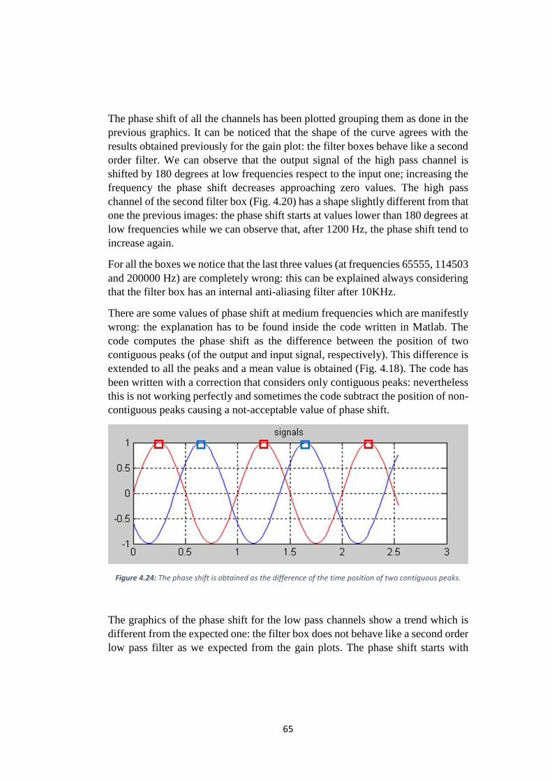
65

The phase shift of all the channels has been plotted grouping them as done in the

previous graphics. It can be noticed that the shape of the curve agrees with the

results obtained previously for the gain plot: the filter boxes behave like a second

order filter. We can observe that the output signal of the high pass channel is

shifted by 180 degrees at low frequencies respect to the input one; increasing the

frequency the phase shift decreases approaching zero values. The high pass

channel of the second filter box (Fig. 4.20) has a shape slightly different from that

one the previous images: the phase shift starts at values lower than 180 degrees at

low frequencies while we can observe that, after 1200 Hz, the phase shift tend to

increase again.

For all the boxes we notice that the last three values (at frequencies 65555, 114503

and 200000 Hz) are completely wrong: this can be explained always considering

that the filter box has an internal anti-aliasing filter after 10KHz.

There are some values of phase shift at medium frequencies which are manifestly

wrong: the explanation has to be found inside the code written in Matlab. The

code computes the phase shift as the difference between the position of two

contiguous peaks (of the output and input signal, respectively). This difference is

extended to all the peaks and a mean value is obtained (Fig. 4.18). The code has

been written with a correction that considers only contiguous peaks: nevertheless

this is not working perfectly and sometimes the code subtract the position of non-

contiguous peaks causing a not-acceptable value of phase shift.

Figure 4.24: The phase shift is obtained as the difference of the time position of two contiguous peaks.

The graphics of the phase shift for the low pass channels show a trend which is

different from the expected one: the filter box does not behave like a second order

low pass filter as we expected from the gain plots. The phase shift starts with

66

values near 0° and decreases up to -300°/-310° rising the frequencies. The last

three values of phase shift for all the boards show a manifestly wrong trend due

to the internal anti-aliasing filter of the box. The results of certain channels

relative to the second filter box are quite rather inaccurate for frequencies higher

than 4032 Hz. In any case it is possible to extrapolate the shape of the filter

obtaining reasonable values of phase shift.

The phase shift in the raw channel should be equal to zero for all the frequencies:

nevertheless, as we can see, this value slightly increases (values lower than 1°) at

higher frequencies. The results related to the second box show some mild

differences among the six channels.

4.1.5 Conclusions

The tests with known input signals have shown some important results useful to

understand the behaviour of filter boxes. It has been verified the type of filter

used, its cut-off frequency and its band-pass. These data processing have led to

some important conclusions on the nature of the filter:

The filter boxes have an internal anti-aliasing filter, with a cut-off

frequency positioned at 10kHZ.

The High-Pass channels are second order high-pass filters: the signal is

attenuated by 40 decibels each decade for frequencies below the cut-off

frequency (100Hz); the phase starts at 180° and decreases to 0° at high

frequencies.

The Low-Pass channels are filters whose cut-off frequency is at 750Hz:

for values higher than fcut-off the signal is attenuated by 40 decibel each

decade. The phase starts at 0° and decreases up to -310°/-320° for

frequencies higher than 10KHz.

The Raw channels behaves correctly reproducing almost perfectly the

input signal: a slight change of phase is evidenced for high frequencies.

67

4.2 Signal compensation

The experiments carried out in the CT3 facility have a short duration (~0.5s). The

compressed air flows through the turbine which rotates at a fixed velocity: the

phenomena analysed in the turbine are unsteady since the flow is extremely fast

and complicated aerodynamic and thermodynamic mechanisms intervene in a

reduced fraction of time. An acceptable experimental analysis can be obtained

only with instrumentations able to sense high frequency fluctuations.

Restarting from the theory described in chapter 3, it has been done a study on the

dynamic behaviour of the cold wire. The calibration conducted in the oven and

inside the heated jet (see Chapter 3) has brought to a relation of the electrical

output of the probe and the stationary physical input (temperature in this case).

The results are valid only for a steady analysis since the output has been taken in

steady conditions.

The dynamic analysis is much more complicated and has to be done using a

physical model which describes the mechanisms occurring close to the wire.

Later, this mathematical approach has to be confirmed by experimental tests to

prove the validity of the model.

In this paragraph it will be explained in detail how it has been possible to

compensate the signal of the cold wire through its transfer function. The

compensation has been done following the works done by Dénos [4] and Arwatz

[5].

4.2.1 Mathematical description of the problem

High speed flow is characterized by high frequency phenomena: the temperature

fluctuation are extremely fast and even the more reliable instruments are not able

to follow these variations. The necessity of the numerical compensation stems

from the knowledge of the physical limits of a probe to sense high frequency

fluctuations. Knowing the characteristics of the probe it is possible to obtain, with

certain approximations, a transfer function that mathematically describes the

dynamic behaviour of the probe. The raw signal sensed by the probe is “filtered”

by the inverse of the transfer function and the compensation is obtained. An

example of the compensated signal is shown in Fig. 4.31. The image comes from

a step test done by Dénos: it can be noticed the recorded signal (raw signal), the

theoretical jet temperature step and the compensated signal.

68

Figure 4.25: Example of a cold wire step signal: through its transfer function it has been compensated and the result is not so different from the ‘real’ jet temperature profile.

4.2.1.1 First order transfer function

The probe has been described mathematically with a first order transfer function.

This result stems from an approximation of the heat exchange mechanisms

occurring near the wire: temperature variations of the probe during the time

depends only on the convective fluxes between air and wire. As a first

approximation it has been neglected the heating caused by the Joule effect and the

conduction phenomena originated by the prongs that hold the wire. These are

some supports usually made of steel whose diameter is several order of magnitude

bigger than that one of the wire. A typical configuration (Fig 4.32) of the cold

wire considers also some smaller stubs between the wire and the prongs in such a

way to reduce conduction phenomena.

Figure 4.26: Configuration of a cold wire: the wire filament is hold by stubs which are connected to some stain prongs.

69

Getting back to the mathematical description of the cold wire done in chapter 3,

the energy balance can be written as follow:

𝑉𝑤𝜌𝑤𝑐𝑤

𝜕𝑇𝑤

𝜕𝑡= −ℎ𝑆𝑤(𝑇𝑤 − 𝑇𝑔)

(4.8)

𝜏

𝜕𝑇𝑤

𝜕𝑡+ 𝑇𝑤 = 𝑓(𝑡) = 𝑇𝑔

(4.9)

𝜏 =𝑉𝑤𝜌𝑤𝑐𝑤

ℎ𝑆𝑤=

𝑑𝑤𝜌𝑤𝑐𝑤

4ℎ being the time constant of the prong, 𝑇𝑔 the gas

temperature, 𝑇𝑤 the wire temperature. It’s first order differential equation that

can be described easily in the frequency domain by its transfer function

𝐻(𝜔) =

1

1 + ϳ𝜔𝜏

(4.10)

Each transfer function can be described by its gain|𝐻(𝜔)| and its phase 𝐻 ̂(𝜔).

An important parameter of a transfer function is the cut-off frequency defined as

the frequency for which |𝐻(𝜔)| = 0.707. It can be easily computed as follow:

𝑓𝑐𝑢𝑡 =

1

2𝜋𝜏

(4.11)

The time constant has been computed in chapter 3. It depends on several

parameter as can be seen in Eq. (4.12): the Nusselt number (expressed as a

function of the Reynolds number) stems from experimental activities that allow

to obtain its constants A, B, n.

𝜏 =

𝑑𝑤2𝜌𝑤

2 𝑐𝑤

4𝑘𝑔 [𝐴 + 𝐵 (𝜌𝑔𝑣𝑔𝑑𝑤

µ𝑔)

𝑛

]

(4.12)

The first order transfer function has been implemented in Matlab considering the

input parameter furnished by Dénos in [4]. In detail, it has been considered a

70

heated jet with velocity 𝑣𝑔 = 25𝑚/𝑠 and total temperature 𝑇𝑔 = 340𝐾: the

experiment has been done at atmospheric pressure. The density of air has been

computed from perfect gas equation, the air being assumed as a perfect gas with

R = 287 J/(kg K) and γ=1.4 ; the viscosity µ𝑔 and conductivity 𝑘𝑔 of air stem from

experimental relations function of the temperature. The data of the wire relative

to density and specific heat ratio come from experimental tables relative to

tungsten. The constant A,B and n are defined with an experimental correlation

that takes into account density and velocity variations. The diameter of the wire

is 2.5 µm. All the data are reported in the following table.

Physical quantity Description/unit Value

𝑣𝑔 [m/s] 25

𝑇𝑡𝑜𝑡 [K] 340

µ𝑔 [kg/(m s)] 0,0000217

𝑘𝑔 [W/(m K)] 0.03

𝑇𝑠 [K]

𝑇𝑠 = 𝑇𝑡𝑜𝑡 − 𝑣𝑔2 2𝐶𝑝⁄

339.8

𝜌𝑔 [kg/𝑚3]

𝜌𝑔 = 𝑃 𝑅 𝑇⁄ 1.0253

𝑑𝑤 [m] 0.0000025

𝜌𝑤 [kg/𝑚3] 20000

𝑐𝑤 [J/(kg K)] 134

A Intercept of experimental

relation Nu(Re) 0.458

B Slope of experimental relation

Nu(Re) 0.345

n Exponent in experimental

relation Nu(Re) 0.45

τ [s] 0.0001369

Table 4.2: Data to compute the first order transfer function

In order to compute the one first order transfer function the only data that have

not been provided were the density of air and the static temperature. As mentioned

before, density has been computed with perfect gas equation while the static

temperature comes from the steady flow energy equation.

The following figures refer to the gain of the transfer function: the first one has

been provided by Dénos in his work while the second one on the right is the

transfer function computed with these data in Matlab.

71

Figure 4.27: Comparison of the computed first order transfer function with the one found by Dénos

The two transfer functions looks like each other: the cut-off frequency found in

Matlab, 𝑓𝑐 = 1162𝐻𝑧 is not so different from that one found by Dénos (𝑓𝑐 =

996𝐻𝑧). This small difference might be due to some differences in the

computation of density or static temperature. The image on the left shows that the

transfer function computed by Dénos perfectly fits with experimental data found

for a 2.5 µm cold wire tested at 25 m/s. For this test Dénos used a frequency

generator in order to test the dynamic response of the wire with a known input (in

this case an input AC current was superimposed to a 10mA DC current). The

experimental part to determine the dynamic behaviour of the wire has not been

done due to a lack of time and to the risk to break the wire.

4.2.1.2 Two first order transfer function

The main source of inaccuracy of the model previously described is that it does

not take into account the conduction phenomena between wire and prongs. Dénos

provides a mathematical description of this mechanism dealing with the steady

and unsteady case. In the steady condition he considers the prongs with an infinite

thermal capacity (the prongs stay at an imposed temperature) while he neglects

the Joule effect. The phenomenon is described by the following equation and its

boundary conditions:

𝜕2𝑇𝑤

𝜕𝑥2= 𝜆2(𝑇𝑤 − 𝑇𝑔)

(4.13)

72

𝑄𝑐𝑜𝑛𝑑 (𝑥 =

𝑙

2) = 0

(4.14)

𝑇𝑤(𝑥 = 0) = 𝑇𝑝

(4.15)

where 𝜆2 =4ℎ

𝑘𝑤 𝑑𝑤, 𝑇𝑔is the gas temperature and 𝑇𝑝 is the temperature of the prong;

x = 0 states one extremity of the wire. This equation has an analytical solution

that allows to compute an important parameter used to define the two first order

transfer function: this parameter is g, defined as 𝑇𝑤(𝑚𝑒𝑎𝑛)−𝑇𝑝

𝑇𝑔−𝑇𝑝. This value is an

index of the heat transferred by convection respect to the whole heat transferred.

Once defined g it is possible to implement the transfer function: this is realized as

the weighted sum of two first order transfer functions. The first transfer

function 𝐻(𝑠) is related to the wire and weighted with parameter g (associated

with convective phenomena); the other transfer function 𝐻𝑝(𝑠) describes the

behaviour of the prong and is weighted with (1-g):

𝐺(𝑠) = 𝑔𝐻(𝑠) + (1 − 𝑔)𝐻𝑝(𝑠)

(4.16)

As a consequence also the probe temperature results in a linear combination of

the wire and prong temperatures.

The wire first order transfer function has been computed using as input parameters

𝑣𝑔 = 100𝑚/𝑠, 𝑇𝑡𝑜𝑡 = 340,15𝐾 and 𝑑𝑤 = 0,0000025𝑚. The time constant 𝜏𝑤

associated to its transfer function is equal to 0,00009227 s.

The prong first order transfer function has been computed using other

experimental values. The prong time constant 𝜏𝑝 is defined as follow:

𝜏𝑝 =

𝑑𝑝2𝜌𝑝𝑐𝑝

4𝑘𝑔 [𝐴𝑝 + 𝐵𝑝 (𝜌𝑔𝑣𝑔𝐿𝑝

µ𝑔)

𝑛𝑝

]

(4.17)

73

It’s possible to notice that the Reynolds number has been defined respect to 𝐿𝑝,

the length of the prong. Moreover, the time constant of the prong has been

computed using a different Nusselt number: the correlation used is the one used

by Paniagua [3] to describe the Nusselt number of air flowing parallel to a wire.

In this case the prong has been assumed as a thicker wire with 𝐿𝑝 as length. All

the data have been reported in the following table:

Physical quantity Description/unit Value

𝑣𝑔 [m/s] 100

𝑇𝑡𝑜𝑡 [K] 340

µ𝑔 [kg/(m s)] 0,0000217

𝑘𝑔 [W/(m K)] 0.03

𝑇𝑠 [K]

𝑇𝑠 = 𝑇𝑡𝑜𝑡 − 𝑣𝑔2 2𝐶𝑝⁄

335

𝜌𝑔 [kg/𝑚3]

𝜌𝑔 = 𝑃 𝑅 𝑇⁄ 1.04

𝑑𝑝 [m] 0.0004

𝜌𝑝 [kg/𝑚3] 7750

𝑐𝑝 [J/(kg K)] 452

𝐴𝑝 Intercept of experimental

relation Nu(Re) 0.085

𝐵𝑝 Slope of experimental relation

Nu(Re) 0.009

𝑛𝑝 Exponent in experimental

relation Nu(Re) 0.674

𝜏𝑝 [s] 1.0547

Figure 4.3: Data used to compute the second order transfer function

The transfer function obtained with the weighted sum of two first order transfer

function is a strictly proper transfer function with degree of denominator higher

than that one of numerator (d=2 > n=1). The value of g used to compute this

transfer function is obtained from an empirical correlation (that will be

mentioned later) and it’s equal to 0.7522. In Fig. 4.34 it’s shown the computed

transfer function and the one provided by Dénos computed using three different

prong time constants. They differ a little especially for the length of the plateau

region (the flat part between the two cut-off frequencies): this might be

explained for the different value of g used in the formula. Dénos does not

provide the value used to compute its transfer function.

74

Figure 4.28: Comparison between the computed second order transfer function with the one found by Dénos

4.2.1.3 Five first order transfer function

The accuracy of the physical model can be improved increasing the number of

first order transfer functions used to obtain the final one. Following the example

of Dénos it has been implemented the code to obtain a five first order transfer

function: the first one is referred to the wire while the remaining ones describe the

behaviour of the prongs.

The transfer function of the probe obtained by Dénos has been experimentally

found with step tests. The time constants and the contributions of each (computed)

first order system to the overall signal are adapted so that the system response to

the reconstructed step fits the experimental response. Knowing the time constants

of the five transfer functions and all the data relative to density, viscosity,

conductivity and velocity of air it is possible to obtain the equivalent diameters.

These data are reported in table 4.4 also with the values of (𝑔𝑖) found

experimentally.

In the Matlab code it has been chosen always the same wire made of tungsten

keeping the characteristics used in the other cases; the heated jet has a total

temperature of 340 K and a velocity of 200 m/s. The density of the gas was found

with the perfect gas equation considering ambient pressure. The time constant of

the wire has been obtained with the same experimental values (A, B, n) used in

the previous cases for the wire transfer function: its value at 200 m/s is equal to

0.00007237 s.

75

The other four transfer functions have been written using the data furnished by

Dénos (see table 4.5): the Reynolds number have been evaluated respect to the

equivalent diameters while the Nusselt number have been defined with a new

correlation:

𝑅𝑒𝑖 =

𝜌𝑔𝑣𝑔 𝑑𝑝𝑖

µ𝑎

(4.18)

𝑁𝑢𝑖 = −6,4511 + 0,438𝑅𝑒𝑖0,45

(4.19)

𝜏𝑝𝑖 =

𝑑𝑝𝑖2𝜌𝑝𝑐𝑝

4𝑘𝑔𝑁𝑢𝑖

(4.20)

Equivalent diameter [mm] Percentage of contribution to (𝟏 − 𝐠)𝒊

0.157 43

0.597 20

0.983 33

2.49 4

Table 4.4: The values of (1-g) have been found experimentally after having obtained the real transfer function. The equivalent diameters are obtained analitically.

Knowing the values of the time constants 𝜏𝑝𝑖 and 𝜏𝑤 it is possible to write the first

order transfer functions in the generic formula and combine them knowing the

values of g and (𝟏 − 𝐠)𝐢 :

𝐻𝑝(𝑠)𝑖 =

1

1 + 𝑠𝜏𝑝𝑖

(4.21)

𝐻(𝑠) =

1

1 + 𝜏𝑤𝑠

(4.22)

𝐺(𝑠) = 𝑔𝐻(𝑠) + ∑(1 − 𝑔)𝑖𝐻𝑝(𝑠)𝑖

4

1

(4.23)

76

The computed transfer function 𝐺(𝑠)is represented in figure with the one by

Dénos. Nevertheless he does not provides the data of the time constants and the

associated cut-off frequencies: it is possible to make only a qualitatively

comparison between them.

The value of g stems from an analytical formula provided by Dénos:

𝑔 = 0.0596𝑅𝑒0.45 + 0.570 (4.23.1)

Physical quantity Description/unit

Value

𝑣𝑔 [m/s] 200

𝑇𝑡𝑜𝑡 [K] 340

µ𝑔 [kg/(m s)] 0,0000217

𝑘𝑔 [W/(m K)] 0.03

𝑇𝑠 [K]

𝑇𝑠 = 𝑇𝑡𝑜𝑡 − 𝑣𝑔2 2𝐶𝑝⁄

320

𝜌𝑔 [kg/𝑚3]

𝜌𝑔 = 𝑃 𝑅 𝑇⁄ 1.088

𝑑𝑝1 [m] 0.000157

𝑑𝑝2 [m] 0.000597

𝑑𝑝3 [m] 0.000983

𝑑𝑝4 [m] 0.00249

𝜌𝑝 [kg/𝑚3] 7750

𝑐𝑝 [J/(kg K)] 452

𝐴 Intercept of experimental

relation Nu(Re) -6,4511

𝐵 Slope of experimental relation

Nu(Re) 0,438

𝑛 Exponent in experimental

relation Nu(Re) 0.45

𝜏𝑤 [s] 0.00007237

𝜏𝑝1 [s] 0.0453

𝜏𝑝2 [s] 0.6555

𝜏𝑝3 [s] 1.7771

𝜏𝑝4 [s] 11.403

Table 4.5: Data used to compute the five first order transfer function.

77

Figure 4.29: Comparison between the computed five first order transfer function and the one obtained by Dénos

As can be seen the computed transfer function looks like to the one referred to

cold wire type A in Fig. 4.35. The value of cut-off frequency associated to the

wire (𝜏𝑤) seems correct being for both the graphic around 1500Hz.

This computational part has been done in order to reproduce the work done by

Dénos and having some ideas of the order of magnitude of the parameters

involved in the dynamic calibration. Next chapter describes the experimental

setup used to realize the dynamic calibration and shows the obtained results.

78

79

Chapter 5

Experimental activity

The experimental activity was firstly focused in finding the real dynamic model

of the cold wire. After having found the transfer functions of the cold wire for

different Mach number the cold wire has been tested inside the CT3 with the

turbine stage working in transient vacuum-ambient pressure conditions.

5.1 Dynamic calibration of the cold wire

The cold wire has been first calibrated in static conditions as described in chapter

3: it has been tested in natural-convection conditions inside the oven and in

forced-convection conditions in a heated jet. As a result we dispose of different

calibration coefficients referred to the cold wire at different Mach numbers ( table

3.4).

The problem of the instruments working in short duration experiments is that they

have to senses physical variations in a small fraction of time. The analysed

phenomena are extremely unstable and the static calibration shows its limits. It is

necessary to develop a real dynamic model that describes the behaviour of the

probe in unsteady conditions and that takes into account all the effects of

conduction of prongs. The theoretical work has been described in the second part

of chapter 4: according to the description provided by Dénos, we developed three

different models for the cold wire using 1,2 and 5 first order transfer functions. It

was possible to make qualitatively conclusions but there was no experimental data

referred to the cold wire.

For this reasons different tests have been done in order to characterize the probe

in unsteady conditions: the cold wire has been tested with step tests realized at

different Mach number and different test durations; the data obtained have been

processed and it was possible to extract the transfer function of the instrument.

The following paragraphs illustrate the experimental procedure used to get these

results and the code realized in order to analyse the data.

80

5.1.1 Experimental setup

For the dynamic calibration it has been chosen the cold wire DAO123A which

has two transducers 1A and 2A placed at the extremity and at the centre of the

probe, respectively. The tests have been done for both the heads but the transfer

function has been computed referring to the results relative to head 1A because

they were more accurate. The probe is shown in Fig. 5.1 and the physical

characteristics and the coefficients of calibration at different Mach number are

reported in Table 5.1.

Probe Head Electronics Mach T = a*V + b

a b R² (0 = oven)

DAO123A 1A Black Box -

CH1

0 29,9297205 21,2746 0,99923

0,05 43,1686293 25,0399 0,99981

0,2 41,6652308 26,8696 0,99922

0,3 43,5803606 19,1749 0,99973

2A White Box -

CH1

0 17,8797016 16,862 0,9993

0,3 25,4295907 24,203 0,9996

Table 5.1: Calibration coefficients of the cold wire at different Mach numbers.

As mentioned before, the tests realized to evaluate the transfer function of the

probe consisted in step tests in which the transducer experienced an abruptly

change of temperature due to the passage of a hot jet. In order to realize these

tests, in addition to the cold wire, two thermocouples and a differential pressure

probe were used. The two thermocouples, 2R and 4R, are the same used in the

static experiment described in chapter 3; the pressure transducer is the 12V8 that

has been calibrated before the test. The coefficients of the calibration are reported

in table 5.2.

81

Figure 5.1: Cold wire DAO123A.

Calibration (P = a*V+b) 12V8 (relative pressure sensor)

a 0.298707271

b 0.125502363

𝑅2 0.999999619

Table 5.2: Calibration coefficients of the pressure transducer 12V8.

As done for the static jet in the heated jet, also in this case it has been used almost

the same experimental setup. The air jet is blown by a nozzle mounted on a

support and linked by pipes to a heat exchanger and to the air reservoir. It was

possible to increase or decrease the temperature of the air using a handle that

changes the current flowing into the resistances of the heat exchanger. The

pressure and total temperature were monitored by the 12V8 Sensym transducer

82

and 4R thermocouple placed inside the nozzle. The thermocouple 2R and the cold

wires were mounted close each other using mechanical supports and placed just

behind the nozzle exit. In order to realize the temperature steps the two probes

(2R and DAO123A) were shielded by a rectangular piece of wood that separated

the nozzle from the transducers. In this case the piece of wood was mounted on a

support that could run along a guide up and down thus exposing the probes to the

hot flow. It was possible to control the moving support through a pneumatic

system that made the wooden shield move only pressing a bottom. The nominal

velocity of the moving support is 0.5 m/s.

Also for this experiment the two thermocouples have been linked to the amplifiers

(2R TC to TU07; 4R TC to TU04); the pressure transducer is the 12V8, powered

by a 15V power supply; the cold wire is linked to a Wheatstone bridge which, in

turn is linked to a power supply. The head 1A, the one on the bottom, is linked to

the black box TUCW3; the head 2A, the one on the middle, is linked to the white

box TUCW2.

These four transducers have been connected to a data acquisition system and to a

computer in order to use a software and set the acquisition parameters. Before

setting the parameters for the acquisition, it has been done a preliminary

computation for the expected maximum and minimum values in the experiment.

In particular, in order to give an adequate sampling rate it has been easily

quantified the test step. Since the nominal velocity of the support is 0.5 m/s and

the diameter of the hole of the nozzle is 12 mm, the expected time necessary to

characterize the step is 24 ms, which is associated to 41.67Hz. In order to respect

the Nyquist criterion, the minimum sampling frequency has to be the double, 83.3

Hz. The modern calculators allow to sample at a far higher frequency rate: the

limit to sample with a high rate is that there is less memory to record data and the

observation time is reduced.

5.1.2 Step tests

The step tests have been realised at different Mach number setting a temperature

difference of 40°C at least. The nominal Mach number decided for the tests are

0.05, 0.1, 0.2 and 0.3. In order to achieve the correct Mach number it must be set

the total pressure value in the air reservoir which is computed with the following

formula:

𝑃𝑡𝑜𝑡 = 𝑃𝑠 [1 + (𝛾 − 1

2) 𝑀2]

𝛾𝛾−1

(5.1)

83

Being 𝑃𝑠 the ambient static pressure and 𝛾 = 1.4. The value was displayed in volt

in a multimeter linked to the pressure transducer 12V8 and the related value in

bar was obtained using the calibration coefficients. Once the temperature of the

air inside the nozzle reached the desired value, it was possible to start the

experiments. The experiments should have been realized at constant ΔT in the

four different tests at different Mach numbers: nevertheless the heating system is

rather simple and it was not possible to set the temperature with accuracy.

In Fig. 5.2 it is possible to see the results from a step test at Mach number 0.05and

jet-total temperature of about 60°C when the head 1A is tested. In the figure the

signals are displayed in Celsius degrees since the calibration coefficients have

been applied. In this case we used the coefficients obtained in static conditions in

the oven test for the 2R (grees), 4R (red) and cold wire (blue) outputs. The 2R

thermocouple and the cold wire show the same temperature in the initial phase

before the step.

Figure 5.2: Step test: the electrical outputs of the 4R (red), 2R (green) and 1A (blues) have been converted into degrees using the calibration coefficients obtained in the still air test (Mach = 0).

84

The test has been done at Mach 0.05 and the calibration coefficients of the cold

wire at that velocity are rather different from those obtained in the oven at Mach

0 (see table. 5.1). The electrical signal of the cold wire has been converted in

degrees with the coefficients obtained in the calibration at Mach 0.05 keeping the

same coefficients for the signals of 2R and 4R thermocouples (coming from a

static calibration in natural convective conditions, i.e. Mach 0). The resulting

temperature curves are displayed in Fig 5.3. In this case, in the initial phase at

constant temperature, the 2R and cold wire transducers show a different

temperature: this difference is due to the use of calibration coefficients coming

from two different type of conditions (natural and forced convections)

Figure 5.3: Step test: the electrical outputs of the 4R (red), 2R (green) have been converted into degrees using the calibration coefficients obtained in the still air test (Mach = 0); the cold wire output (blue) has been converted with calibration coefficients obtained in a test at Mach = 0.05.

Nevertheless it has been decided to use these last coefficients (referring to the

forced convection) subtracting the temperature shift existing between the two

curves and obtaining the results depicted in the following figure.

85

Figure 5.4: For all the step tests it has been decided to use the static calibration coefficients at Mach=0 for the 2R and 4R thermocouples. The cold wire output has been modified with coefficients of calibration relative to the correct Mach number subtracting a shift of temperature.

The signal, especially the one of the cold wire, is extremely noisy: before doing

any qualitative analysis it has been cleaned using a digital low pass filter. The

high peaks observed at around 0 seconds are due to the drop of electric current

occurring when the bottom controlling the shield movement is pressed.

5.1.2.1 First step test

A first step test has been done using a sampling frequency of 8000Hz and an

observation time of 8 seconds. In the following pictures it has been plotted the

cold wire signal relative to head 1A (filtered and cleaned from the spurious peaks),

the 2R and 4R signals in function of time for different Mach numbers. As

mentioned before, due to the inaccuracy of the heating system it was not possible

to set easily the step temperature to a fixed value in the four tests. The cold wire

signal has been filtered with a Butterworth filter of the fourth order and a cut-off

frequency of 10Hz.

86

Figure 5.5: Step test 1 at Mach 0.05

Figure 5.6: Step test 1 at Mach 0.1

87

Figure 5.7: Step test 1 at Mach 0.2

Figure 5.8: Step test 1 at Mach 0.3

88

The reactivity of head 1A of the cold wire is much higher than the one of the

thermocouple 2R in the initial phase of the step. However the thermocouple seems

reaching a stable final value while the cold wire curve has a final positive slope.

It needs some more time to reach a stable final value. A second step test has been

done increasing the observation time and modifying slightly the position of the

probes.

5.1.2.2 Second step test

In this test it has been decided to place the 2R thermocouple and the cold wire

head 1A as close as possible each-others in such a way that they could sense the

same temperature variations. Moreover, the two transducers have been placed

closer to the exit of the nozzle in such a way to reduce the heat losses. A picture

of the “modified” setup is shown in Fig. 5.9. For this experiment we changed the

sampling frequency reducing it from 8000 to 4000Hz in order to increase the

observation time: finally the step test was analysed for about 16 seconds without

affecting significantly the accuracy of the sampling.

Figure 5.9: The setup used to realize the step tests. The two probes are shielded by a rectangular piece of wood that closes the flow blown by the nozzle.

89

Figure 5.10: Step test 2 at Mach 0.05

Figure 5.11: Step test 1 at Mach 0.1

90

Figure 5.12: Step test 2 at Mach 0.2

Figure 5.13: Step test 2 at Mach 0.3

91

The first thing that can be observed is that doubling the observation time allows

to get curves with a final stable value. Nevertheless the curves of head 1A of the

cold wire at low Mach numbers (0.05, 0.1) show always a slight positive final

slope, which means that the velocity of the flow interferes on the reactivity of the

probe. In any way, the new setup and a longer observation time brought to better

results: the final temperature registered by the cold wire and 2R thermocouple are

closer respect to the first case. The difference of temperature existing between the

two probes and the “nominal” total temperature sensed inside the nozzle can be

explained with the velocity error described in chapter 3. While the 4R

thermocouple placed inside the nozzle senses the total temperature of the flux at

extremely low velocity, the two probes placed outside are submerged into a flow

of a certain velocity. The flow around the probes is not brought to rest

isentropically but, due to the viscous stresses and heat losses, the conversion of

kinetic energy into thermal enthalpy is incomplete and the total temperature

registered by the probes immersed in the flow is lower than the nominal stagnation

temperature.

Since the second step test give better results, the research of the experimental

transfer function will be lead using these last data referred to the head 1A of the

cold wire.

5.2 Compensation of the signal

The necessity to compensate the signal has been explained in the previous chapter

where it has been illustrated the concept of transfer function of a probe. In

particular, it has been described how to compute transfer functions of different

orders.

The compensation of the signal is a technique used to overcome the physical

limits of a transducer to react to external unsteady excitations. In effect, each

transducer is characterized by a static behaviour, related to the ability to reproduce

the response of a stationary input and a dynamic behaviour which allows to get

the response of the probe to unsteady inputs. Once the dynamic behaviour of the

probe is known, knowing its transfer function, the compensation is obtained

simply applying the inverse of its transfer function to the signal.

The aim of this experimental work is to obtain the experimental transfer function

of head 1A of the cold wire DAO123A starting from the outputs sampled in the

second step tests previously described. Three approaches will be described in

92

order to compute the transfer function and it will be chosen the one that gives the

more reliable results.

5.2.1 FFT ratio approach

The most known technique used to compute an experimental transfer function

consists in doing the ratio between the Fast Fourier Transform (FFT) of the output

signal and the FFT of the input signal:

𝐻(𝜔) =

𝑌(𝜔)

𝑋(𝜔)

(5.2)

In our experiment, the output 𝑌(𝜔) is the Fourier transform of the recorded cold

wire signal while the input 𝑋(𝜔) is the Fourier transform of the theoretical step.

The cold wire signal, tested in this case at Mach 0.05 for 14 seconds, has been

filtered with a Butterworth low-pass filter of the fourth order with a cut-off

frequency of 10 Hz and has been adimensionalized in this manner:

𝑇𝑎𝑑 =

𝑇𝑐𝑤 − min (𝑇𝑐𝑤)

max(𝑇𝑐𝑤) − 𝑚𝑖𝑛(𝑇𝑐𝑤)

(5.3)

The two signals (output and input) are depicted in Fig. 5.14. The problem of this

technique is that it can be used when the input signal has a Fast Fourier Transform

whose values are above a certain minimum value. In this case the input signal is

a step and the Fourier transform of a step has values close to zero as the frequency

increases (see Fig 5.15). For this reasons when dividing the two vectors 𝑌(𝜔) and

𝑋(𝜔) the resulting transfer function shows meaningless peaks that makes the

results unusable (see Fig. 5.16).

93

Figure 5.14: Comparison between the cold wire step signal and the theoretical Heaviside step.

Figure 5.15: Fast Fourier Transform of the cold wire signal (blue) and of the Heaviside signal (red).

94

The resulting transfer function is shown in the following picture.

Figure 5.16: The ratio of the FFT of the cold wire signal and the FFT of the Heaviside input signal gives the experimental transfer function

5.2.2 Differentiation approach

The step tests are generally easy to realize in the practice: the problem is that their

results cannot be used directly to obtain the transfer function of the transducer.

Another alternative to obtain an experimental transfer function is to “redefine”

the step-time signal: this is differentiated, subtracting two consecutively values of

the step signal and dividing each by the delta time between them. What we obtain

is, as expected, an impulse signal because the impulse is the derivative of the step.

The resulting signal is shown in the following picture.

95

Figure 5.17: The impulse signal has been obtained subtracting two consecutively values of the original step signal and dividing this value by the delta time between them.

The advantage of using this technique is that when we want to apply the Fourier

Fast transform to the theoretical impulse signal we obtain one, from the theory. In

this case, being the FFT of the input 𝑋(𝜔) = 1, the experimental transfer function

coincides with the FFT of the output 𝑌(𝜔).

𝐻(𝜔) = 𝑌(𝜔) (5.4)

The FFT of the differentiated signal produce this transfer function:

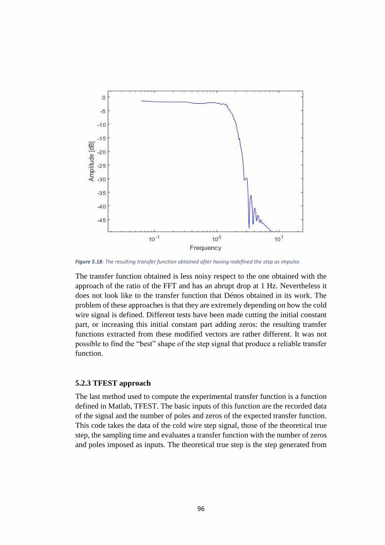
96

Figure 5.18: The resulting transfer function obtained after having redefined the step as impulse.

The transfer function obtained is less noisy respect to the one obtained with the

approach of the ratio of the FFT and has an abrupt drop at 1 Hz. Nevertheless it

does not look like to the transfer function that Dénos obtained in its work. The

problem of these approaches is that they are extremely depending on how the cold

wire signal is defined. Different tests have been made cutting the initial constant

part, or increasing this initial constant part adding zeros: the resulting transfer

functions extracted from these modified vectors are rather different. It was not

possible to find the “best” shape of the step signal that produce a reliable transfer

function.

5.2.3 TFEST approach

The last method used to compute the experimental transfer function is a function

defined in Matlab, TFEST. The basic inputs of this function are the recorded data

of the signal and the number of poles and zeros of the expected transfer function.

This code takes the data of the cold wire step signal, those of the theoretical true

step, the sampling time and evaluates a transfer function with the number of zeros

and poles imposed as inputs. The theoretical true step is the step generated from

97

the movement of finite velocity of the wooden shield (0.5 m/s in this case). In Fig.

5.19 it is shown the theoretical true step and theoretical step (Heaviside).

Figure 5.19: The theoretical true step is the step generated by the movement of the shield. Since the nozzle has a diameter of 12 mm and the support moves the shield at a finite velocity, 0.5 m/s, the step lasts 0.024 seconds.

The details of the code are not available: it tries to compute an analytical transfer

function that best matches the transfer function that it finds experimentally with

the data. The output it’s a transfer function characterized by a “Fit to estimation

data” value: it is a percentage that shows how much the computed transfer

function reproduces the behaviour of the experimental one.

It has been written a code that loads the experimental results of the step test of the

cold wire. The signal has been cleaned from the spurious peaks, low-pass filtered

and adimensionalized as described before: it is shown in the following picture.

98

Figure 5.20: The signal of the cold wire has been cleaned from spurious peaks, low-pass filtered and adimnesionalized.

The modified data have been used to compute the transfer function with ‘tfest’.

According with the work done by Dénos, the transfer functions used to describe

the probe are of the first, second and fifth order. For this work it has been chosen

to test the data imposing a second, third, fourth and fifth order transfer functions

(selecting two, three, four, five poles respectively in the options of ‘tfest’). The

transfer functions obtained at Mach 0.05 are depicted in figure.

Figure 5.21: The experimental transfer functions found with ‘tfest’ with a different number of poles with tests at Mach number 0.05

99

Among the four transfer functions, the one that gives the higher ‘Fit to estimation

data’ value is the 3rd order transfer function with 96.45%. The experimental

transfer functions seem describing correctly the behaviour at low frequency: the

effect of the conduction of the prongs is visible in the magnitude bode diagram

with the small steps and with a reduction of the amplitude of the output. The

abruptly drop of magnitude at around 10 Hz is due to the finite probe injection

speed (0.5 m/s) and to the existence of a shear layer on both sides of the jet: these

combined effects allow to analyse only phenomena in a restricted field of

frequencies. This result is not sufficient to obtain a realistic dynamic description

of the cold wire. The main element of the probe, the tungsten wire, is not taken

into account in this analysis.

The wire, as widely descripted in chapter three, behaves as a first order system

and it is possible to evaluate its transfer function with a formula that includes

experimental data of Reynolds number, Nusselt number, physical and geometrical

data of the wire (density, diameter). It is the main element of the probe that permits

to sense high frequency fluctuations: its contribute in the experimental transfer

function is not visible since the step experiments allow to analyse only the low

frequencies phenomena.

In order to obtain a realistic description of the dynamic phenomena we decided to

combine the results of the experimental transfer function (related to low

frequencies phenomena, i.e. conductions of prongs) and those obtained

analytically (with the first order transfer function). In the following picture it’s

depicted the experimental transfer function obtained with ‘tfest’ imposing two

poles and one zeros (TF), the first order transfer function obtained analytically

(TF_1ORDER) and the transfer function that combines both (TF_mod).

100

Figure 5.22: The modified transfer function (TF_mod) combines the low frequency behaviour of the experimental transfer function found with ‘tfest’ and the high frequency behaviour which stems from the dynamic behaviour of the tungsten wire (described with a first order transfer function).

The blue transfer function (TF in the picture) has been modified artificially

substituting the pole at 1Hz with the one found in the first order transfer function

with cut-off frequency of about 1000Hz. The resulting transfer function is the red

one (TF_mod).

One source of inaccuracy of the obtained transfer function has to be found in the

value of the cut-off frequency of the tungsten wire: this has not experimentally

computed. Not disposing of the experimental setup we found this value

analytically with formula provided by Dénos and described previously in chapter

4.

The transfer functions used in this test at Mach 0.3 are here reported:

𝐺1(𝑠) =

11472.79

𝑠 + 11472.79

(5.5)

101

𝐺2(𝑠) =

𝑠 + 0.6675

(𝑠 + 92.914)(𝑠 + 0.52833)

(5.6)

𝐺2𝑚𝑜𝑑(𝑠) =

(𝑠 + 0.6675)(𝑠 + 1000000)

(𝑠 + 11472.79)(𝑠 + 0.52833)

(5.7)

In the modified transfer function 𝐺2𝑚𝑜𝑑(𝑠) we added a high frequency zero at

1MHz in order to obtain a proper transfer function that can be reversed without

modify its shape before that value of frequency.

The main limit of this method is that it does not take into account what happens

in the plateau region. Realizing step tests with a higher injection velocity of the

shield (in this case it was 0.5 m/s) it is possible to analyse the dynamic behaviour

in a wider range of frequencies.

The transfer functions found at Mach 0.3 have been modified adding the cut-off

frequency of the tungsten wire (equal to 1

2𝜋𝜏). The results are depicted in Fig. 5.23.

Figure 5.23: The transfer functions found with ‘tfest’ imposing different numbers of poles in step tests at Mach number 0.3.

102

The 3rd order transfer function is the one that gives the higher ‘Fit to estimation

data value’. The analytical expression (which stems from a step test at Mach =

0.3) is here reported:

𝐺(𝑠) =

0.007686𝑠3 + 7686𝑠2 + 59280𝑠 + 28000

𝑠3 + 11480𝑠2 + 72280𝑠 + 28000

(5.9)

This transfer function has been inverted and used to compensate the cold wire

signal in order to reproduce the theoretical step; in Fig. 5.24 is shown the original

signal of the cold wire, the reconstructed step and the theoretical step. The figure

on the bottom (Fig. 5.25) shows the computed transfer function in blue and the

inverse transfer function in red. The reconstructed signal was obtained doing the

FFT of the cold wire signal and multiplying this outcome with the vector resulting

from the ‘freqresp’ function. This function has as inputs the inverse of the transfer

function and the frequency range expressed in radians.

Figure 5.24: The cold wire signal has been compensated using the inverse of the transfer function. The reconstructed step fits well the theoretical true step.

103

Figure 5.25: The transfer function (blue) and it inverse (red) used for the compensation.

5.2.4 Conclusions

The step tests realized with the moving support allowed to get the experimental

transfer function of head 1A of the cold wire DAO123A.

The transfer function is defined in three parts: the low frequency part described

with the transfer function obtained with ‘tfest’; the medium frequency part which

is approximate with a flat region; the high frequency part defined starting from

the cut-off frequency found with a first order transfer function.

As mentioned before, the main limit of this approach is the undefined medium

region which has been approximate as flat. A higher injection velocity of the

support would allow to find the real behaviour in this medium frequency region.

The cut-off frequency of the tungsten wire stems from an analytical formula but

no experimental tests have been realised to confirm this trend.

The other two methods used to compute the transfer function gave erroneous

results. They are extremely dependant on how the step vector has been defined.

104

The obtained 3rd order TF has been used to compensate the cold wire step signal.

The results are good: the compensated signal well fits the theoretical one. For the

test in turbine will be generated four transfer functions of the 3rd order at different

Mach number (0.05, 0.1, 0.2, 0.3) in such a way to see the differences of the

compensated signal in the four cases.

5.3 Cold wire test in CT3

The CT3 is a facility in Von Karman Institute used to test turbine stages in

similarity conditions with aero-engines. It has been done an experiment to

understand the effect of energy dissipation due to the injection of air at ambient

pressure in the settling chamber. The rotor is brought to a stable rotating velocity

in a vacuum ambient and it is analysed how the injection of air affects the working

conditions when it rotates only for inertia.

5.3.1 Description of the test

It has been analysed the transient phenomena occurring when the turbine, initially

rotating in vacuum ambient at constant speed, encounters flow at ambient

pressure.

The turbine test section has been equipped by several instruments to sense

pressure and temperature variations. First of all the turbine test section has been

brought to vacuum (under 30mbar absolute pressure). The rotor of the turbine is

spun up to the desired speed by an auxiliary power turbine, for this test at about

2200 rpm. As a stable value of rotating speed is reached, the power turbine is

turned off: the rotor keeps rotating for inertia always in vacuum conditions.

Several valves are opened: air at ambient temperature and pressure enters in the

turbine test section and the aero-brakes are activated. Due to the increase of

pressure and density inside the chamber the rotors experiences drag and the aero-

brakes produce an opposite momentum respect to the direction of rotation. After

few minutes the rotor is brought to rest; rpm, temperature and pressure conditions

are monitored during all the test.

The aim of the test is to use the cold wire which has been calibrated for static and

dynamic conditions and understand which mechanisms intervene during the

transient replenishment phase.

105

5.3.2 Experimental setup

The main facility for this test is the CT3 test rig. The complete description is

provided in chapter two: it’s a facility used to test turbine stages in aero-engines

working conditions. A light piston of 1.6 m of diameter can course inside a 8

meters long cylinder: from the back of the piston some pressurized air is provided

thus generating a pressure difference in the two chambers separated by the piston

itself. An isentropic compression is realised: as the air inside the second chamber

of the piston reaches the desired temperature and pressure a valve is opened and

the compressed air is blown in the test chamber. The turbine to be tested is rotating

at a certain speed and for a short time the flow passes through it. During the test

several instruments are used to register some parameters. In our experiment the

CT3 has been used to bring the turbine to a desired velocity (2200 rpm) in vacuum

conditions. A vacuum pump has been used to reach a total pressure under 30 mbar.

In order to understand the mechanisms occurring during the open-valves-phase it

has been used the cold wire DAO123A, described in the previous chapters and 3

differential pressure probes. All the four transducers have been placed inside the

CT3, behind the rotor.

The electronic used for the cold wire DAO123A is always the same used during

the calibration: head 1A has been linked to the black box TUCW3, head 2A has

been linked to the white box TUCW2. The cold wire outputs have been connected

to the Wheatstone bridge through a longer cable: it has been registered a higher

value of resistance respect the one obtained registered during the calibration of

cold wire. This will results in a shift of the electrical output. This effect has to be

taken into account in order to get a correct conversion voltage-temperature.

The DAO123A is a cold wire which has been calibrated in static and dynamic

conditions. It has two heads, one placed in the middle and the other at the

extremity of the probe (respectively head 2A and head 1A). The CT3 facility is

designed in order to easily insert transducers: in effect there are some holes

realised for this purpose. The DAO123A can be mounted into the facility through

a metallic support which is depicted in Fig. 5.26. The metallic piece, named 3904-

46, is pierced with 5 holes with 8 millimeters of diameter and the probe can be

easily inserted having a slightly smaller diameter. The assembly of the probe can

be quite complicated due to the extreme fragility of the wire: for this purpose it

has been used the tool descripted in chapter 2.

106

Figure 5.26: The probes are inserted in these metallic supports which, in turn, are inserted in the CT3 facility.

The objective is to fix the probe at the correct height and angle in the turbine

channel trying to move as less as possible the transducer. The metallic support is

mounted on the tool and the variable-height instrument is placed under the tool as

depicted in Fig. 5.27. With the Excel program descripted in chapter two it is

possible to set the correct eight of the variable-height instrument in such a way to

obtain the correct value of deep of the probe inside the turbine channel. The probe

courses inside the metallic support till it touches the surface of the variable-height-

tool. For this experiment head 1A, the one placed at the extremity of the probe

DAO123A, has been inserted at 75% of the total length of the turbine channel

with a 0° angle (computed respect to the axis of the turbine).

Figure 5.27: The setup used to set the depth and the angle of the probe in the turbine channel.

107

The pressure transducers used in this experiment are always differential pressure

transducers, as the other used in other tests. In this case the SENSYMs are the

SENSA1, SENSA2 and SENSA3. These probes have been calibrated with the

process descripted in chapter 3 and the following tables are referred to the values

of slope and intercept obtained after the calibration.

Calibration (P = a*V+b) SENSA1 (relative pressure sensor)

A -540.22

b 1621.844

𝑅2 0.999976

Calibration (P = a*V+b) SENSA2 (relative pressure sensor)

A -551.788

b 1661.067

𝑅2 0.999992412

Calibration (P = a*V+b) SENSA3 (relative pressure sensor)

A -543.423

b 1634.398

𝑅2 0.99998555

Table 5.3: Calibration coefficients of the differential pressure probes SENSA1, SENSA2 and SENSA3.

Another transducer has been used to compute the round per minutes of the turbine

in order to have a graphic of the velocity of rotor during the test.

The 5 probes have been linked to GENESIS the data acquisition system used also

for the analogue filter tests, described in the first part of chapter four. In this test

we acquired the signals for 192 seconds with a sampling frequency of 5000 Hz.

A low pass filter with a cut-off frequency of 500 Hz has been used. The head 1A

of cold wire DAO123A has been sampled at 5000 Hz (for the whole duration, 192

seconds) and also at 200000 Hz (for a shorter duration). For the higher sampling

frequency case we used a low-pass filter with a cut-off frequency of 50000Hz.

The aim of this double sampling was to get the differences of the cold wire signal

during the unsteady phase (at the opening of the valves). Due to a setting error the

108

higher sampling signal has been recorded in the wrong period and we recorded a

stable (high sampled) signal.

5.3.3 Test and results

The test has a length of almost 5 minutes since the rotor needs to be spun up to

2200 rpm. When the desired rotating speed is reached the data acquisition system

starts acquiring data for a total length of 3 minutes. The test ends when the turbine

is brought to zero velocity due to the intervention of the aero-brakes after the

injection of air. The results of the experiment are reported in the following graphs.

The first images analysed are those referred to the velocity of rotor and to the

trend of pressure inside the test chamber.

Figure 5.28: The RPM during the test in the turbine rig.

109

Figure 5.29: The pressure sensed by the differential pressure transducers during the test in the turbine rig.

It can be noticed that in the first 40 seconds the measured quantities are constant:

the RPM sensor displays 2200 revolutions per minute and the three differential

pressure probes have a low constant value. The sensor SENSA2 shows a slight

shift of almost 2000 Pascal respect to the other probes: this can be due to

electronics. At 40 seconds the valves are opened and the pressure inside the test

chamber increases linearly during 50 seconds while the rotor, which is rotating

only for inertia, starts decelerating. The turbine stops rotating and the pressure is

monitored one minute more: after having reached a stable value for few seconds,

pressure slowly decreases to the final ambient pressure (94495 Pa).

The results of the cold wire are shown in the following pictures. One is referred

to head 1A, placed more deeply in the turbine channel (75% of the total length of

the channel); the second one, head 2A, is placed at 25% of the total length of the

channel. As mentioned before, the probe has been linked to the Wheatstone bridge

through a cable which has a higher electrical resistance respect to the one used

during the calibrations: this results in a shift of the temperature. Knowing the

ambient temperature by a thermometer and the initial temperature registered by

110

the cold wire (in the first 40 seconds) it is possible to find the shift. The corrected

results are plotted here below.

Figure 5.30: Comparison of the signals of the two heads of cold wire DAO123A

The initial temperature is almost the same for both the transducers (there is a

difference of less than 1 degree). The physical phenomenon of kinetic energy

dissipation (observed previously with the RPM graphic) can be interpreted in

another way with the graphics of the cold wire. We observe that, as the valves are

opened at 40 seconds, the temperature registered by the cold wire rises abruptly:

the air enters in the chamber and is accelerated by the movement of the rotor. In

this phase there is a conversion of kinetic energy of the turbine into thermal energy

of air. During this phase the kinetic energy of the turbine decreases due to the

effect of aero-brakes which generates an opposite momentum respect to the

rotation. As the RPM decreases also the conversion of kinetic energy decreases:

after the abrupt peak, the temperature decreases. We can observe that the

temperature sensed by the two sensors is different during the open-valve-phase:

head 1A, which is the transducer placed at the extremity (i.e. at a lower radial

distance from the axe of the turbine), senses a lower temperature respect to the

111

other head. This result can be related to a difference of kinetic energy: the

tangential velocity of air increases with the radius from the axis of the turbine.

Since head 2A has a radial distance greater respect to the one of head 1A, the air

impacting on this first probe will have a higher kinetic energy, which will result

in a higher total temperature. In both graphics, that have been plotted together in

figure, we observe a similar phenomenon between 115 and 135 seconds. In this

phase the turbine decelerate from 35 RPM to 0 and temperature registered from

both the transducers increases slightly. In the last minute of recording, when the

RPM is 0, temperature slowly increases from 16°C to 17°C while the pressure

stabilises to the final ambient pressure value.

5.3.4 Compensation of the cold wire

Once obtained the results of cold wire DAO123A we tried to compensate the

signal registered from head 1A using the transfer functions obtained with the step

tests. The abrupt open of the valves is associated with the peak of temperature

which occurs in a small fraction of time (~0.05s). In order to compensate the

signal we used the transfer functions of 3rd order (those one that gave the highest

‘Fit to estimation data’ value) obtained at different Mach number (0.05, 0.1, 0.2,

0.3): the transfer functions are shown in the following figure.

112

Figure 5.31: The transfer function of 3rd obtained with the step tests for different Mach numbers. It is possible to see the effect of velocity on the shape of the transfer function.

It can be noticed that the four transfer functions have a similar shape with a cut-

off frequency of the wire at around 1000Hz. The increase of Mach number causes

a higher convection which results in a faster response of the probe. The transfer

function has been inverted and, through the use of the ‘lsim’ function in Matlab,

it was possible to obtain the compensation of the signal of head 1A of the probe.

The results of the raw signal and the compensated one are shown in Fig. 5.32.

Later, the signal has been filtered with a fourth order low-pass Butterworth filter

with a cut-off frequency of 5 Hz. The compensation has been applied to this

filtered signal with the four inverse transfer functions and the results are depicted

in figures 5.33, 5.34, 5.35, 5.36.

113

Figure 5.32: Comparison of the raw signal of the cold wire and the compensated raw signal of the cold wire (head 1A with a transfer function obtained in a step test at Mach = 0.05).

The transfer functions that have been applied to compensate the signal stem from

step tests realized at different Mach numbers. All the step tests have been realised

with a known time constant equal to 0.024 seconds. This time constant is obtained

as the ratio of the diameter of the nozzle injecting air and the velocity of the

variable height support. The time constant of the experiment in the CT3 is about

0.05 seconds (this value has been checked manually in the four tests and it is

referred to the time required to reach the peak of temperature). The two

experiments (step test and test in CT3) have a time constants of the same order: it

is interesting to see how the Mach number influences the compensation. As

observed in Fig. 5.31, the transfer functions differ among them and the effect of

velocity (i.e. convection) interferes on the shape of the transfer function. This

means that it does not exist a unique transfer function that can describe a dynamic

phenomenon in all the frequencies: there is a certain dependence on the velocity

of the flow. The question is which transfer function is more adapted to compensate

the cold wire tested in the CT3.

114

Figure 5.33: Compensation with the transfer function obtained at Mach= 0.05.

Figure 5.34: Compensation with the transfer function obtained at Mach= 0.1.

115

Figure 5.35: Compensation with the transfer function obtained at Mach= 0.2.

Figure 5.36: Compensation with the transfer function obtained at Mach= 0.3.

116

The test in CT3 has been done to test the cold wire in transient conditions when

air at ambient pressure is injected in the test chamber and the turbine is rotating

in vacuum conditions. The cold wire has to sense temperature variations in a

different condition respect to the test done for the calibration. In effect the step

test it’s easy to be described: the air has a certain temperature, Mach number and

impacts the cold wire perpendicularly as a narrow heated jet. The fluid dynamic

inside the CT3 during this test is much more complicated and would deserve

another study since we deal with a transient phenomenon from vacuum to ambient

pressure conditions. The air enters in the chamber and two main events occur

simultaneously: the ‘chaotic’ expansion inside the test chamber and the

interaction of the flow with the rotating turbine. The flow impacting on the cold

wire is not a jet with a known direction and velocity. A correct analysis should

take into account the velocity and direction of the flow hitting the probe but no

other transducers have been used in this test. For this reason the description of the

results will be qualitative.

They are visible four different phases of this test: the first part at vacuum

conditions; the second one when air is injected and impact the aero-brakes causing

the rotor to decelerate; the third one when the rotor is brought to rest; the fourth

one when air expands uniformly in the chamber without the interference of the

rotor. The final temperature is lower respect the ambient temperature but we can

see that it’s not the final stable value (it’s required a longer acquisition). There are

some differences in the four compensated signals: the one with the highest peak

at 40 seconds is the signal compensated with the transfer function obtained in the

step test at Mach 0.05; as the Mach number increases the same peak is less

compensated (has a smaller amplitude) and the compensated signal approaches

the raw one. Aside from this peak, there are no significant differences in the

compensation among the cases at different Mach number: the cold wire responds

rather accurately also without compensation. We can conclude that for these tests

the use of a transfer function respect to another is rather indifferent since the Mach

number does not play an important influence. The cold wire is enough fast to

reproduce the temperature in this kind of test. It would be interesting to see how

behaves the cold wire in experiments with a smaller time constant using the same

transfer functions used in this test (which has a time constant of 0.024 seconds).

117

5.3.5 Conclusions

The test in the CT3 has highlighted the effects of heating caused by the interaction

of air with the rotor. After the abrupt peak caused by the contact of the turbine

with air, the total temperature sensed by the cold wire decreases with the velocity

of the rotor: the test chamber is slowly filled by air at ambient pressure which

causes the rotor to decelerate.

The effect of compensation in this test are not particularly visible: the fast peak

of temperature experienced at the opening of valves is compensated using four

different transfer functions (obtained in step tests at 4 different Mach number and

same time constant). The difference of temperature of the compensated signal

respect to the raw signal is of about 1-2 degrees which means that the cold wire

is enough fast for this test. The differences in the four compensations are not so

clear: the more suitable transfer function should be the one that has been obtained

in conditions similar to those experienced during the test in CT3. This comparison

is not possible not disposing of enough accurate information of the flow around

the cold wire.

A better characterization of the dynamic behaviour of the cold wire would be

obtained realizing step tests with a lower step time constant (i.e higher injection

velocity). It would be interesting to test these transfer functions for faster

phenomena, for example increasing the velocity of the rotor and generating a

higher and a faster temperature peak.

118

119

Bibliography

[1] IATA Economic Briefing. Airline Fuel and Labour cost share. February 2010

[2] J. Anthoine, T. Arts, H.L. Boerrigter, J.-M. Buchlin, M. Carbonaro, G. Degrez,

R. Denos, D. Fletcher, D. Olivari, M.L. Riethmuller, R.A. Van den

Braembussche, Measurement techniques in fluid dynamics, An introduction

[3] G. Paniagua, R. Dénos, M. Oropesa, Thermocouple probes for accurate

temperature measurements in short duration facilities, April 2002

[4] R. Dénos, Sieverding CH (1997) Assessment of the cold wire resistance

thermometer for high speed turbomachinery applications. Transactions of ASME:

J. Turbomach 119: 1140-148

[5] Gilad Arwatz, Carla Bahri, Alexander J Smits and Marcus Hultmark, 28

August 2013. Dynamic calibration and modelling of a cold wire for temperature

measurements. Mechanical and Aerospace Engineering. Princeton University,

USA.

[6] D. Sergio Lavagnoli, DR. D. José Marìa Desantes, DR. D. Guillermo

Paniagua, On the Aerothermal Flow Field in a Transonic HP Turbine Stage with

a Multi-Profile LP Stator Vane.

120

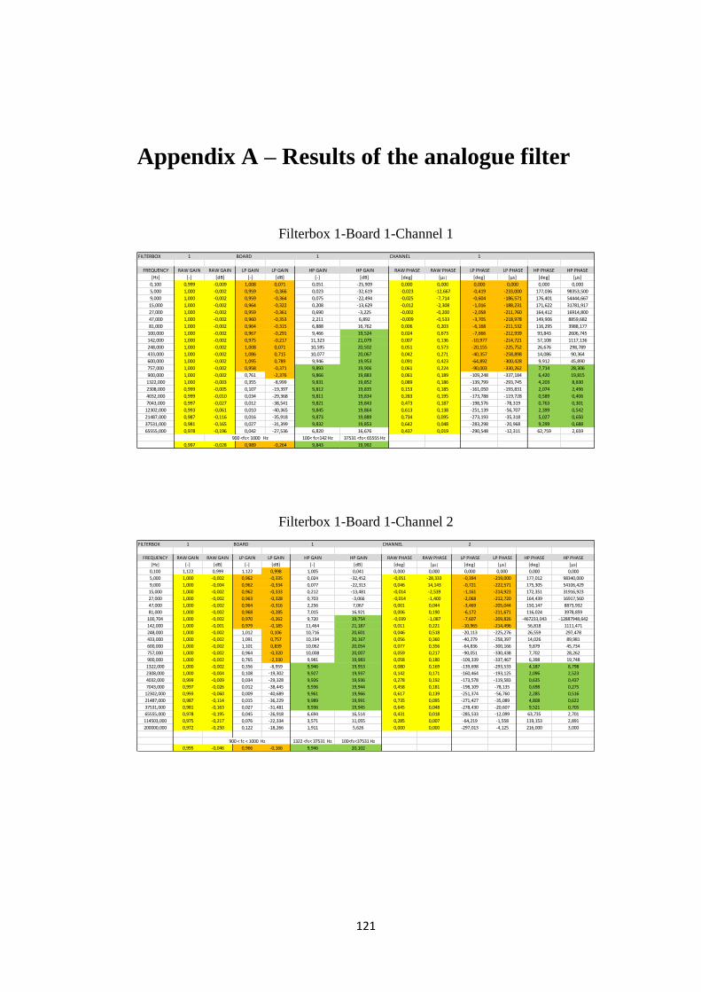
121

Appendix A – Results of the analogue filter

Filterbox 1-Board 1-Channel 1

Filterbox 1-Board 1-Channel 2

FILTERBOX 1 BOARD 1 CHANNEL 1

FREQUENCY RAW GAIN RAW GAIN LP GAIN LP GAIN HP GAIN HP GAIN RAW PHASE RAW PHASE LP PHASE LP PHASE HP PHASE HP PHASE

[Hz] [-] [dB] [-] [dB] [-] [dB] [deg] [µs ] [deg] [µs] [deg] [µs]

0,100 0,999 -0,009 1,008 0,071 0,051 -25,909 0,000 0,000 0,000 0,000 0,000 0,000

5,000 1,000 -0,002 0,959 -0,366 0,023 -32,619 -0,023 -12,667 -0,419 -233,000 177,036 98353,500

9,000 1,000 -0,002 0,959 -0,364 0,075 -22,494 -0,025 -7,714 -0,604 -186,571 176,401 54444,667

15,000 1,000 -0,002 0,964 -0,322 0,208 -13,629 -0,012 -2,308 -1,016 -188,231 171,622 31781,917

27,000 1,000 -0,002 0,959 -0,361 0,690 -3,225 -0,002 -0,200 -2,058 -211,760 164,412 16914,800

47,000 1,000 -0,002 0,960 -0,353 2,211 6,892 -0,009 -0,533 -3,705 -218,978 149,906 8859,682

81,000 1,000 -0,002 0,964 -0,315 6,888 16,762 0,006 0,203 -6,168 -211,532 116,295 3988,177

100,000 1,000 -0,002 0,967 -0,291 9,466 19,524 0,024 0,673 -7,666 -212,939 93,843 2606,745

142,000 1,000 -0,002 0,975 -0,217 11,323 21,079 0,007 0,136 -10,977 -214,721 57,108 1117,136

248,000 1,000 -0,002 1,008 0,071 10,595 20,502 0,051 0,573 -20,155 -225,752 26,676 298,789

433,000 1,000 -0,002 1,086 0,715 10,077 20,067 0,042 0,271 -40,357 -258,898 14,086 90,364

600,000 1,000 -0,002 1,095 0,789 9,946 19,953 0,091 0,423 -64,892 -300,428 9,912 45,890

757,000 1,000 -0,002 0,958 -0,371 9,893 19,906 0,061 0,224 -90,003 -330,262 7,714 28,306

900,000 1,000 -0,002 0,761 -2,376 9,866 19,883 0,061 0,189 -109,248 -337,184 6,420 19,815

1322,000 1,000 -0,003 0,355 -8,999 9,831 19,852 0,089 0,186 -139,799 -293,745 4,203 8,830

2308,000 0,999 -0,005 0,107 -19,397 9,812 19,835 0,153 0,185 -161,050 -193,831 2,074 2,496

4032,000 0,999 -0,010 0,034 -29,368 9,811 19,834 0,283 0,195 -173,788 -119,728 0,589 0,406

7043,000 0,997 -0,027 0,012 -38,541 9,821 19,843 0,473 0,187 -198,576 -78,319 0,763 0,301

12302,000 0,993 -0,061 0,010 -40,365 9,845 19,864 0,613 0,138 -251,139 -56,707 2,399 0,542

21487,000 0,987 -0,116 0,016 -35,918 9,873 19,889 0,734 0,095 -273,193 -35,318 5,027 0,650

37531,000 0,981 -0,165 0,027 -31,399 9,832 19,853 0,642 0,048 -283,298 -20,968 9,299 0,688

65555,000 0,978 -0,196 0,042 -27,536 6,820 16,676 0,437 0,019 -290,548 -12,311 62,759 2,659

900 <fc< 1000 Hz 100< fc<142 Hz 37531 <fc< 65555 Hz

0,997 -0,028 0,989 -0,264 9,843 19,992

FILTERBOX 1 BOARD 1 CHANNEL 2

FREQUENCY RAW GAIN RAW GAIN LP GAIN LP GAIN HP GAIN HP GAIN RAW PHASE RAW PHASE LP PHASE LP PHASE HP PHASE HP PHASE

[Hz] [-] [dB] [-] [dB] [-] [dB] [deg] [µs ] [deg] [µs] [deg] [µs]

0,100 1,122 0,999 1,122 0,998 1,005 0,041 0,000 0,000 0,000 0,000 0,000 0,000

5,000 1,000 -0,002 0,962 -0,335 0,024 -32,452 -0,051 -28,333 -0,394 -219,000 177,012 98340,000

9,000 1,000 -0,004 0,962 -0,334 0,077 -22,313 0,046 14,143 -0,721 -222,571 175,305 54106,429

15,000 1,000 -0,002 0,962 -0,333 0,212 -13,481 -0,014 -2,539 -1,161 -214,923 172,351 31916,923

27,000 1,000 -0,002 0,963 -0,328 0,703 -3,066 -0,014 -1,400 -2,068 -212,720 164,439 16917,560

47,000 1,000 -0,002 0,964 -0,316 2,256 7,067 0,001 0,044 -3,469 -205,044 150,147 8873,932

81,000 1,000 -0,002 0,968 -0,285 7,015 16,921 0,006 0,190 -6,172 -211,671 116,024 3978,859

100,704 1,000 -0,002 0,970 -0,262 9,720 19,754 -0,039 -1,087 -7,607 -209,826 -467233,043 -12887948,642

142,000 1,000 -0,001 0,979 -0,185 11,464 21,187 0,011 0,221 -10,965 -214,496 56,818 1111,471

248,000 1,000 -0,002 1,012 0,106 10,716 20,601 0,046 0,518 -20,113 -225,276 26,559 297,478

433,000 1,000 -0,002 1,091 0,757 10,194 20,167 0,056 0,360 -40,279 -258,397 14,026 89,981

600,000 1,000 -0,002 1,101 0,839 10,062 20,054 0,077 0,356 -64,836 -300,166 9,879 45,734

757,000 1,000 -0,002 0,964 -0,320 10,008 20,007 0,059 0,217 -90,051 -330,438 7,702 28,262

900,000 1,000 -0,002 0,765 -2,330 9,981 19,983 0,058 0,180 -109,339 -337,467 6,398 19,748

1322,000 1,000 -0,002 0,356 -8,959 9,946 19,953 0,080 0,169 -139,698 -293,533 4,187 8,798

2308,000 1,000 -0,004 0,108 -19,302 9,927 19,937 0,142 0,171 -160,464 -193,125 2,096 2,523

4032,000 0,999 -0,009 0,034 -29,328 9,926 19,936 0,278 0,192 -173,578 -119,583 0,635 0,437

7043,000 0,997 -0,026 0,012 -38,445 9,936 19,944 0,458 0,181 -198,109 -78,135 0,698 0,275

12302,000 0,993 -0,060 0,009 -40,689 9,961 19,966 0,617 0,139 -251,374 -56,760 2,285 0,516

21487,000 0,987 -0,114 0,015 -36,229 9,989 19,991 0,735 0,095 -271,427 -35,089 4,808 0,622

37531,000 0,981 -0,163 0,027 -31,481 9,936 19,945 0,645 0,048 -278,430 -20,607 9,521 0,705

65555,000 0,978 -0,195 0,045 -26,918 6,694 16,514 0,431 0,018 -285,533 -12,099 63,735 2,701

114503,000 0,975 -0,217 0,076 -22,334 3,571 11,055 0,285 0,007 -64,219 -1,558 119,153 2,891

200000,000 0,972 -0,250 0,122 -18,266 1,911 5,626 0,000 0,000 -297,013 -4,125 216,000 3,000

900 < fc < 1000 Hz 1322 <fc< 37531 Hz 100<fc<37531 Hz

0,995 -0,046 0,966 -0,166 9,946 20,102

122

Filterbox 1-Board 1-Channel 3

Filterbox 1-Board 1-Channel 4

FILTERBOX 1 BOARD 1 CHANNEL 3

FREQUENCY RAW GAIN RAW GAIN LP GAIN LP GAIN HP GAIN HP GAIN RAW PHASE RAW PHASE LP PHASE LP PHASE HP PHASE HP PHASE

[Hz] [-] [dB] [-] [dB] [-] [dB] [deg] [µs ] [deg] [µs] [deg] [µs]

0,100 1,000 0,000 0,951 -0,435 0,041 -27,727 0,000 0,000 0,000 0,000 0,000 0,000

5,000 1,000 -0,001 0,913 -0,787 0,022 -32,988 0,021 11,667 -0,403 -223,667 178,291 99050,667

9,000 1,000 -0,002 0,914 -0,784 0,072 -22,858 -0,022 -6,714 -0,690 -213,000 174,316 53801,167

15,000 1,000 -0,002 0,914 -0,785 0,200 -13,980 -0,006 -1,154 -1,149 -212,692 173,379 32107,167

27,000 1,000 -0,001 0,914 -0,780 0,663 -3,564 0,015 1,560 -2,079 -213,840 164,191 16892,083

47,000 1,000 -0,002 0,915 -0,769 2,124 6,542 0,000 -0,022 -3,257 -192,511 150,096 8870,909

81,000 1,000 -0,002 0,919 -0,736 6,589 16,377 0,010 0,354 -6,154 -211,051 115,854 3973,051

100,000 1,000 -0,002 0,921 -0,711 9,024 19,108 0,021 0,571 -7,656 -212,653 93,434 2595,398

142,000 1,000 -0,002 0,929 -0,637 10,781 20,653 0,008 0,150 -11,016 -215,493 57,033 1115,679

248,000 1,000 -0,002 0,960 -0,350 10,118 20,102 0,048 0,541 -20,140 -225,577 26,737 299,472

433,000 1,000 -0,002 1,034 0,289 9,634 19,676 0,055 0,353 -40,389 -259,102 14,130 90,647

600,000 1,000 -0,002 1,043 0,362 9,512 19,565 0,086 0,396 -64,859 -300,273 9,952 46,074

757,000 1,000 -0,002 0,913 -0,793 9,461 19,519 0,049 0,180 -89,985 -330,195 7,762 28,483

900,000 1,000 -0,002 0,725 -2,790 9,436 19,496 0,051 0,157 -109,078 -336,661 6,439 19,872

1322,000 1,000 -0,002 0,339 -9,396 9,404 19,466 0,087 0,183 -139,513 -293,143 4,222 8,871

2308,000 1,000 -0,004 0,103 -19,724 9,386 19,450 0,158 0,190 -160,459 -193,119 2,089 2,515

4032,000 0,999 -0,010 0,033 -29,731 9,385 19,449 0,286 0,197 -172,951 -119,152 0,607 0,418

7043,000 0,997 -0,026 0,011 -38,991 9,395 19,458 0,445 0,175 -196,256 -77,404 0,725 0,286

12302,000 0,993 -0,061 0,008 -42,103 9,419 19,480 0,614 0,139 -249,711 -56,384 2,368 0,535

21487,000 0,987 -0,115 0,013 -37,728 9,447 19,506 0,744 0,096 -273,811 -35,397 4,967 0,642

37531,000 0,981 -0,164 0,023 -32,881 9,425 19,485 0,640 0,047 -284,201 -21,035 8,997 0,666

65555,000 0,978 -0,195 0,039 -28,231 6,767 16,607 0,441 0,019 -290,115 -12,293 60,552 2,566

900 < fc <1000 Hz 900<fc<37531 Hz 100<fc< 37531 Hz

0,997 -0,027 0,925 -0,693 9,412 19,601

FILTERBOX 1 BOARD 1 CHANNEL 4

FREQUENCY RAW GAIN RAW GAIN LP GAIN LP GAIN HP GAIN HP GAIN RAW PHASE RAW PHASE LP PHASE LP PHASE HP PHASE HP PHASE

[Hz] [-] [dB] [-] [dB] [-] [dB] [deg] [µs ] [deg] [µs] [deg] [µs]

0,100 1,122 0,998 1,118 0,967 1,005 0,040 0,000 0,000 0,000 0,000 0,000 0,000

5,000 1,000 -0,002 0,929 -0,643 0,022 -32,963 -0,042 -23,500 -0,455 -252,750 180,050 100027,500

9,000 1,000 -0,002 0,929 -0,642 0,073 -22,689 0,008 2,429 -0,680 -209,857 174,814 53955,000

15,000 1,000 -0,002 0,929 -0,640 0,202 -13,900 0,016 2,923 -1,154 -213,769 171,756 31806,692

27,000 1,000 -0,002 0,929 -0,637 0,671 -3,462 0,011 1,120 -2,059 -211,880 164,263 16899,500

47,000 1,000 -0,001 0,931 -0,621 2,155 6,669 0,012 0,733 -3,422 -202,267 150,277 8881,622

81,000 1,000 -0,002 0,934 -0,592 6,688 16,506 0,013 0,456 -6,149 -210,861 115,571 3963,329

100,000 1,000 -0,002 0,937 -0,568 9,143 19,222 0,018 0,490 -7,635 -212,092 92,958 2582,153

142,000 1,000 -0,002 0,945 -0,494 10,854 20,712 0,017 0,332 -10,940 -214,007 56,514 1105,514

248,000 1,000 -0,002 0,977 -0,204 10,149 20,129 0,047 0,524 -20,032 -224,378 26,457 296,341

433,000 1,000 -0,002 1,053 0,446 9,660 19,700 0,053 0,343 -40,173 -257,717 13,991 89,758

600,000 1,000 -0,002 1,063 0,534 9,536 19,588 0,079 0,366 -64,671 -299,401 9,853 45,614

757,000 1,000 -0,002 0,932 -0,613 9,486 19,541 0,074 0,273 -89,884 -329,825 7,668 28,139

900,000 1,000 -0,002 0,740 -2,613 9,460 19,518 0,059 0,183 -109,107 -336,749 6,369 19,658

1322,000 1,000 -0,002 0,345 -9,242 9,428 19,488 0,087 0,183 -139,677 -293,489 4,168 8,757

2308,000 1,000 -0,004 0,105 -19,607 9,410 19,472 0,151 0,182 -161,092 -193,882 2,063 2,483

4032,000 0,999 -0,010 0,033 -29,650 9,409 19,471 0,287 0,198 -177,156 -122,049 0,595 0,410

7043,000 0,997 -0,026 0,013 -37,716 9,418 19,479 0,464 0,183 -213,998 -84,402 0,747 0,295

12302,000 0,993 -0,060 0,015 -36,427 9,443 19,502 0,610 0,138 -261,856 -59,127 2,354 0,532

21487,000 0,987 -0,114 0,026 -31,602 9,471 19,528 0,739 0,096 -276,739 -35,776 4,946 0,639

37531,000 0,981 -0,163 0,044 -27,130 9,444 19,503 0,640 0,047 -285,844 -21,156 9,243 0,684

65555,000 0,978 -0,195 0,067 -23,526 6,522 16,288 0,441 0,019 -293,089 -12,419 62,951 2,667

114502,000 0,975 -0,217 0,079 -22,007 3,472 10,811 0,286 0,007 -36,522 -0,886 239,707 5,815

200000,000 0,971 -0,253 0,108 -19,361 1,990 5,978 0,287 0,004 -6,357 -0,088 190,411 2,645

900 < fc <1000 900 < fc < 37531 Hz 100 <fc < 37531

1,000 -0,004 0,938 -0,452 9,435 19,632

123

Filterbox 1-Board 2-Channel 1

Filterbox 1-Board 2-Channel 2

FILTERBOX 1,000 BOARD 2,000 CHANNEL 1,000

FREQUENCY RAW GAIN RAW GAIN LP GAIN LP GAIN HP GAIN HP GAIN RAW PHASE RAW PHASE LP PHASE LP PHASE HP PHASE HP PHASE

[Hz] [-] [dB] [-] [dB] [-] [dB] [deg] [µs ] [deg] [µs] [deg] [µs]

0,100 1,122 1,000 1,125 1,022 1,003 0,030 0,000 0,000 0,000

5,000 1,000 -0,001 0,989 -0,099 0,023 -32,907 -0,002 -1,333 -0,336 -186,667 174,248 96804,500

9,000 1,000 -0,002 0,988 -0,101 0,074 -22,627 0,002 0,714 -0,725 -223,857 175,866 54279,714

15,000 1,000 -0,001 0,989 -0,098 0,205 -13,785 0,013 2,385 -1,198 -221,923 171,782 31811,461

27,000 1,000 -0,002 0,989 -0,095 0,679 -3,357 -0,002 -0,160 -2,036 -209,440 164,126 16885,440

47,000 1,000 -0,002 0,990 -0,086 2,178 6,761 -0,009 -0,556 -3,704 -218,933 149,787 8852,644

81,000 1,000 -0,002 0,994 -0,051 6,770 16,612 -0,001 -0,037 -6,185 -212,089 116,193 3984,679

100,000 1,000 -0,002 0,997 -0,025 9,294 19,364 -0,006 -0,163 -7,692 -213,673 93,762 2604,490

142,000 1,000 -0,001 1,006 0,049 11,120 20,922 0,012 0,229 -11,046 -216,086 57,136 1117,686

248,000 1,000 -0,002 1,039 0,336 10,421 20,358 0,045 0,502 -20,298 -227,358 26,729 299,380

433,000 1,000 -0,002 1,119 0,974 9,916 19,927 0,061 0,390 -40,605 -260,490 14,112 90,529

600,000 1,000 -0,002 1,126 1,030 9,788 19,814 0,081 0,375 -65,235 -302,015 9,943 46,033

757,000 1,000 -0,002 0,982 -0,155 9,736 19,768 0,062 0,226 -90,324 -331,442 7,751 28,442

900,000 1,000 -0,002 0,779 -2,175 9,710 19,744 0,065 0,200 -109,481 -337,904 6,425 19,831

1322,000 1,000 -0,002 0,363 -8,795 9,676 19,714 0,090 0,189 -139,699 -293,535 4,212 8,850

2308,000 1,000 -0,004 0,111 -19,130 9,657 19,697 0,134 0,161 -160,547 -193,226 2,090 2,515

4032,000 0,999 -0,010 0,035 -29,168 9,656 19,696 0,281 0,194 -173,646 -119,630 0,609 0,420

7043,000 0,997 -0,026 0,012 -38,410 9,665 19,704 0,458 0,181 -200,421 -79,047 0,725 0,286

12302,000 0,993 -0,060 0,010 -40,159 9,691 19,727 0,606 0,137 -252,180 -56,942 357,660 80,759

21487,000 0,987 -0,114 0,017 -35,619 9,718 19,752 0,741 0,096 -274,458 -35,481 4,909 0,635

37531,000 0,981 -0,163 0,028 -30,921 9,684 19,721 0,624 0,046 -283,258 -20,965 8,910 0,659

65555,000 0,978 -0,194 0,045 -26,908 6,833 16,692 0,441 0,019 -289,965 -12,287 61,361 2,600

114503,000 0,975 -0,217 0,067 -23,493 3,632 11,202 0,289 0,007 -311,106 -7,547 117,264 2,845

200000,000 0,971 -0,253 0,095 -20,414 2,055 6,255 0,264 0,004 -338,010 -4,695 192,621 2,675

900<fc<1000 Hz 81< fc < 100 Hz 37531<fc<65555 Hz

0,995 -0,046 0,998 0,038 9,682 19,851

FILTERBOX 1,000 BOARD 2,000 CHANNEL 2,000

FREQUENCY RAW GAIN RAW GAIN LP GAIN LP GAIN HP GAIN HP GAIN RAW PHASE RAW PHASE LP PHASE LP PHASE HP PHASE HP PHASE

[Hz] [-] [dB] [-] [dB] [-] [dB] [deg] [µs ] [deg] [µs] [deg] [µs]

0,100 1,122 1,001 1,121 0,994 1,004 0,032 0,000 0,000 0,000

5,000 1,000 -0,002 0,969 -0,269 0,021 -33,541 0,018 9,750 -0,369 -204,750 180,587 100326,333

9,000 1,000 -0,003 0,969 -0,269 0,068 -23,301 -0,007 -2,286 -0,604 -186,571 174,908 53983,833

15,000 1,000 -0,003 0,969 -0,269 0,190 -14,429 -0,001 -0,154 -1,131 -209,385 172,099 31870,231

27,000 1,000 -0,002 0,970 -0,264 0,630 -4,012 -0,007 -0,760 -2,061 -212,080 164,392 16912,760

47,000 1,000 -0,002 0,972 -0,251 2,025 6,127 -0,028 -1,644 -3,653 -215,889 150,332 8884,864

81,000 1,000 -0,002 0,975 -0,221 6,334 16,033 0,007 0,253 -6,200 -212,620 116,410 3992,115

100,000 1,000 -0,002 0,978 -0,196 8,711 18,801 0,010 0,265 -7,704 -214,010 93,723 2603,408

142,000 1,000 -0,001 0,986 -0,124 10,377 20,321 0,012 0,243 -11,080 -216,750 56,757 1110,279

248,000 1,000 -0,002 1,018 0,157 9,663 19,702 0,045 0,504 -20,289 -227,256 26,421 295,931

433,000 1,000 -0,002 1,093 0,776 9,179 19,256 0,039 0,253 -40,567 -260,244 13,960 89,555

600,000 1,000 -0,002 1,099 0,819 9,058 19,140 0,082 0,380 -65,021 -301,022 9,825 45,485

757,000 1,000 -0,002 0,960 -0,353 9,008 19,093 0,058 0,212 -89,934 -330,008 7,660 28,107

900,000 1,000 -0,002 0,763 -2,345 8,983 19,069 0,060 0,186 -108,989 -336,386 6,347 19,589

1322,000 1,000 -0,002 0,358 -8,922 8,951 19,038 0,089 0,187 -139,290 -292,675 4,165 8,752

2308,000 1,000 -0,004 0,109 -19,233 8,934 19,021 0,146 0,175 -160,200 -192,808 2,088 2,513

4032,000 0,999 -0,009 0,034 -29,257 8,933 19,020 0,285 0,196 -173,343 -119,422 0,632 0,435

7043,000 0,997 -0,026 0,012 -38,373 8,942 19,029 0,466 0,184 -197,620 -77,942 0,672 0,265

12302,000 0,993 -0,060 0,010 -40,325 8,967 19,053 0,614 0,139 -249,430 -56,321 2,215 0,500

21487,000 0,987 -0,114 0,016 -35,945 8,995 19,080 0,734 0,095 -269,817 -34,881 4,713 0,609

37531,000 0,982 -0,162 0,027 -31,226 8,988 19,073 0,630 0,047 -276,342 -20,453 8,870 0,657

65555,000 0,978 -0,194 0,047 -26,566 6,885 16,759 0,438 0,019 -282,809 -11,984 55,087 2,334

114503,000 0,975 -0,216 0,077 -22,275 3,639 11,221 0,292 0,007 -65,161 -1,581 110,772 2,687

200000,000 0,971 -0,256 0,136 -17,347 1,987 5,966 0,267 0,004 -330,755 -4,594 174,168 2,419

900 < fc < 1000 81<fc<100 Hz 37531<fc<65555 Hz

0,995 -0,046 0,979 -0,130 8,962 19,193

124

Filterbox 1-Board 2-Channel 3

Filterbox 1-Board 2-Channel 4

FILTERBOX 1 BOARD 2 CHANNEL 3

FREQUENCY RAW GAIN RAW GAIN LP GAIN LP GAIN HP GAIN HP GAIN RAW PHASE RAW PHASE LP PHASE LP PHASE HP PHASE HP PHASE

[Hz] [-] [dB] [-] [dB] [-] [dB] [deg] [µs ] [deg] [µs] [deg] [µs]

0,100 1,122 1,001 1,122 1,003 1,004 0,032 0,000 0,000 0,000 0,000

5,000 1,000 -0,002 0,969 -0,277 0,023 -32,655 -0,010 -5,667 -0,436 -242,333 177,179 98432,500

9,000 1,000 -0,003 0,969 -0,277 0,076 -22,435 -0,022 -6,714 -0,711 -219,571 174,874 53973,429

15,000 1,000 -0,002 0,969 -0,275 0,210 -13,574 0,023 4,308 -1,174 -217,461 171,235 31710,167

27,000 1,000 -0,001 0,969 -0,272 0,696 -3,153 0,019 1,960 -2,082 -214,160 164,318 16905,167

47,000 1,000 -0,001 0,971 -0,254 2,230 6,965 -0,007 -0,422 -3,445 -203,600 150,675 8905,136

81,000 1,000 -0,001 0,974 -0,228 6,934 16,820 0,004 0,139 -6,222 -213,380 116,478 3994,430

100,000 1,000 -0,001 0,977 -0,202 9,538 19,589 0,012 0,347 -7,734 -214,845 94,102 2613,939

142,000 1,000 -0,001 0,985 -0,130 11,452 21,177 0,009 0,186 -11,091 -216,964 57,406 1122,957

248,000 1,000 -0,001 1,018 0,155 10,739 20,620 0,041 0,455 -20,332 -227,728 26,850 300,736

433,000 1,000 -0,002 1,094 0,782 10,217 20,187 0,040 0,258 -40,648 -260,765 14,164 90,868

600,000 1,000 -0,002 1,100 0,828 10,085 20,073 0,079 0,366 -65,198 -301,844 9,981 46,209

757,000 1,000 -0,002 0,960 -0,356 10,030 20,026 0,058 0,213 -90,237 -331,119 7,778 28,540

900,000 1,000 -0,002 0,762 -2,365 10,003 20,003 0,065 0,202 -109,350 -337,499 6,454 19,921

1322,000 1,000 -0,002 0,356 -8,962 9,968 19,972 0,088 0,184 -139,572 -293,268 4,228 8,885

2308,000 1,000 -0,004 0,109 -19,277 9,950 19,956 0,147 0,176 -160,316 -192,947 2,098 2,525

4032,000 0,999 -0,009 0,034 -29,292 9,948 19,955 0,282 0,195 -173,207 -119,328 0,622 0,428

7043,000 0,997 -0,026 0,012 -38,593 9,958 19,964 0,452 0,178 -196,939 -77,673 0,731 0,288

12302,000 0,993 -0,059 0,008 -41,456 9,985 19,987 0,615 0,139 -248,837 -56,187 2,367 0,535

21487,000 0,987 -0,113 0,014 -37,157 10,012 20,011 0,737 0,095 -273,419 -35,347 4,968 0,642

37531,000 0,982 -0,162 0,024 -32,276 9,973 19,977 0,631 0,047 -283,600 -20,990 349,812 25,891

65555,000 0,978 -0,193 0,042 -27,536 6,663 16,473 0,432 0,018 -286,870 -12,156 295,051 12,502

114503,000 0,975 -0,216 0,078 -22,181 3,548 11,001 0,285 0,007 -305,921 -7,421 121,519 2,948

200000,000 0,972 -0,251 0,101 -19,956 1,850 5,342 0,000 0,000 -10,866 -0,151 154,374 2,144

900<fc<1000 81<fc<100 Hz 37531<fc<65555 Hz

0,995 -0,046 0,978 -0,133 9,969 20,107

FILTERBOX 1 BOARD 2 CHANNEL 4

FREQUENCY RAW GAIN RAW GAIN LP GAIN LP GAIN HP GAIN HP GAIN RAW PHASE RAW PHASE LP PHASE LP PHASE HP PHASE HP PHASE

[Hz] [-] [dB] [-] [dB] [-] [dB] [deg] [µs ] [deg] [µs] [deg] [µs]

0,100 1,122 1,001 1,119 0,977 1,003 0,028 0,000 0,000 0,000 0,000

5,000 1,000 -0,002 0,945 -0,493 0,023 -32,782 0,023 13,000 -0,561 -311,667 175,978 97765,667

9,000 1,000 -0,002 0,945 -0,493 0,073 -22,699 -0,013 -4,000 -0,691 -213,286 176,559 54493,667

15,000 1,000 -0,001 0,945 -0,493 0,204 -13,824 0,011 2,077 -1,124 -208,231 171,888 31831,167

27,000 1,000 -0,002 0,945 -0,489 0,675 -3,412 -0,007 -0,720 -2,035 -209,400 164,237 16896,800

47,000 1,000 -0,002 0,946 -0,478 2,167 6,718 -0,001 -0,044 -3,679 -217,444 149,830 8855,222

81,000 1,000 -0,001 0,950 -0,444 6,731 16,561 0,010 0,329 -6,153 -211,025 116,154 3983,342

100,000 1,000 -0,002 0,953 -0,420 9,239 19,312 0,014 0,378 -7,622 -211,714 93,722 2603,402

142,000 1,000 -0,001 0,961 -0,344 11,049 20,866 0,004 0,071 -10,947 -214,143 57,105 1117,079

248,000 1,000 -0,002 0,994 -0,051 10,351 20,300 0,053 0,589 -20,076 -224,870 26,709 299,159

433,000 1,000 -0,002 1,072 0,606 9,849 19,868 0,051 0,329 -40,297 -258,513 14,102 90,469

600,000 1,000 -0,002 1,083 0,693 9,723 19,756 0,077 0,355 -64,901 -300,470 9,937 46,005

757,000 1,000 -0,002 0,947 -0,473 9,670 19,709 0,062 0,229 -90,225 -331,075 7,750 28,440

900,000 1,000 -0,002 0,750 -2,493 9,644 19,686 0,064 0,197 -109,505 -337,978 6,432 19,853

1322,000 1,000 -0,002 0,349 -9,147 9,611 19,655 0,092 0,192 -139,940 -294,042 4,210 8,847

2308,000 1,000 -0,004 0,106 -19,522 9,593 19,639 0,144 0,173 -161,313 -194,147 2,079 2,503

4032,000 0,999 -0,009 0,033 -29,571 9,592 19,638 0,282 0,194 -177,542 -122,315 0,608 0,419

7043,000 0,997 -0,026 0,013 -37,565 9,601 19,647 0,448 0,177 -216,356 -85,331 0,713 0,281

12302,000 0,993 -0,059 0,016 -35,988 9,627 19,670 0,608 0,137 -262,911 -59,365 2,360 0,533

21487,000 0,987 -0,113 0,028 -31,102 9,655 19,695 0,742 0,096 -276,562 -35,753 4,960 0,641

37531,000 0,982 -0,162 0,047 -26,610 9,623 19,666 0,636 0,047 -284,840 -21,082 9,506 0,704

65555,000 0,978 -0,193 0,071 -22,937 6,573 16,356 0,435 0,018 -292,890 -12,411 63,555 2,693

114503,000 0,975 -0,216 0,085 -21,372 3,500 10,882 0,294 0,007 -41,577 -1,009 120,556 2,925

200000,000 0,971 -0,252 0,113 -18,939 1,992 5,986 0,261 0,004 -3,846 -0,053 192,018 2,667

900< fc <1322 81<fc<100 Hz 37531<fc<65555 Hz

0,995 -0,046 0,954 -0,314 9,618 19,793

125

Filterbox 1-Board 3-Channel 1

Filterbox 1-Board 3-Channel 2

FILTERBOX 1 BOARD 3 CHANNEL 1

FREQUENCY RAW GAIN RAW GAIN LP GAIN LP GAIN HP GAIN HP GAIN RAW PHASE RAW PHASE LP PHASE LP PHASE HP PHASE HP PHASE

[Hz] [-] [dB] [-] [dB] [-] [dB] [deg] [µs ] [deg] [µs] [deg] [µs]

0,100 1,122 1,001 1,121 0,991 1,003 0,029 0,000 0,000 0,000 0,000 0,000 0,000

5,000 1,000 -0,003 0,954 -0,412 0,023 -32,818 -0,004 -2,333 -0,505 -280,667 177,518 98621,000

9,000 1,000 -0,001 0,954 -0,409 0,073 -22,699 -0,020 -6,286 -0,624 -192,571 176,850 54583,429

15,000 1,000 -0,001 0,954 -0,409 0,203 -13,837 0,005 1,000 -1,294 -239,539 173,554 32139,692

27,000 1,000 -0,002 0,955 -0,404 0,674 -3,426 0,017 1,800 -2,077 -213,640 164,443 16918,040

47,000 1,000 -0,002 0,955 -0,396 2,163 6,702 0,001 0,044 -3,452 -204,000 150,440 8891,273

81,000 1,000 -0,002 0,959 -0,363 6,772 16,614 -0,008 -0,291 -6,185 -212,089 116,700 4002,063

100,000 1,000 -0,001 0,962 -0,337 9,333 19,401 0,017 0,469 -7,617 -211,582 94,110 2614,163

142,000 1,000 -0,001 0,970 -0,264 11,168 20,960 0,001 0,014 -10,979 -214,763 57,109 1117,164

248,000 1,000 -0,001 1,002 0,019 10,417 20,355 0,030 0,341 -20,116 -225,313 26,586 297,785

433,000 1,000 -0,001 1,078 0,650 9,896 19,909 0,053 0,339 -40,215 -257,984 14,026 89,981

600,000 1,000 -0,002 1,087 0,725 9,765 19,793 0,074 0,341 -64,563 -298,903 9,876 45,722

757,000 1,000 -0,002 0,954 -0,414 9,711 19,745 0,051 0,187 -89,518 -328,483 7,700 28,254

900,000 1,000 -0,002 0,759 -2,393 9,684 19,721 0,064 0,196 -108,749 -335,645 6,381 19,695

1322,000 1,000 -0,002 0,356 -8,978 9,649 19,690 0,093 0,196 -139,266 -292,624 4,182 8,786

2308,000 1,000 -0,004 0,108 -19,312 9,631 19,673 0,147 0,176 -160,421 -193,074 2,071 2,493

4032,000 0,999 -0,009 0,034 -29,354 9,629 19,672 0,292 0,201 -173,629 -119,619 0,605 0,417

7043,000 0,997 -0,026 0,012 -38,489 9,639 19,680 0,447 0,176 -200,204 -78,961 0,701 0,276

12302,000 0,993 -0,059 0,010 -40,366 9,664 19,703 0,603 0,136 -254,410 -57,445 2,319 0,524

21487,000 0,987 -0,113 0,016 -35,731 9,692 19,728 0,733 0,095 -274,466 -35,482 4,866 0,629

37531,000 0,982 -0,161 0,028 -30,977 9,671 19,709 0,635 0,047 -284,002 -21,020 8,895 0,658

65555,000 0,978 -0,193 0,045 -27,026 7,074 16,994 0,437 0,019 -288,923 -12,243 59,017 2,501

114503,000 0,975 -0,215 0,065 -23,692 3,759 11,501 0,295 0,007 -48,489 -1,176 114,463 2,777

200000,000 0,971 -0,251 0,090 -20,877 1,952 5,810 0,000 0,000 -12,884 -0,179 208,328 2,893

900 < fc < 1000 81< fc < 100 Hz 37531 < fc < 65555 Hz

0,995 -0,046 0,963 -0,244 9,649 19,839

FILTERBOX 1 BOARD 3 CHANNEL 2

FREQUENCY RAW GAIN RAW GAIN LP GAIN LP GAIN HP GAIN HP GAIN RAW PHASE RAW PHASE LP PHASE LP PHASE HP PHASE HP PHASE

[Hz] [-] [dB] [-] [dB] [-] [dB] [deg] [µs ] [deg] [µs] [deg] [µs]

0,100 1,122 1,000 1,124 1,013 1,004 0,034 0,000 0,000 0,000 0,000 0,000 0,000

5,000 1,000 0,000 0,974 -0,226 0,023 -32,655 -0,011 -6,000 -0,484 -269,000 174,899 97166,333

9,000 1,000 -0,001 0,975 -0,224 0,075 -22,466 -0,014 -4,429 -0,600 -185,143 174,635 53899,714

15,000 1,000 -0,002 0,975 -0,223 0,209 -13,615 -0,001 -0,154 -1,096 -203,000 170,303 31537,667

27,000 1,000 -0,001 0,975 -0,219 0,691 -3,210 -0,009 -0,880 -2,027 -208,520 164,110 16883,792

47,000 1,000 -0,001 0,976 -0,208 2,213 6,900 -0,012 -0,689 -3,492 -206,400 150,019 8866,400

81,000 1,000 -0,001 0,980 -0,175 6,854 16,719 0,016 0,544 -6,107 -209,418 115,771 3970,190

100,000 1,000 -0,001 0,983 -0,150 9,381 19,445 0,000 0,010 -7,579 -210,520 93,380 2593,898

142,000 1,000 -0,001 0,991 -0,076 11,205 20,988 0,008 0,150 -10,928 -213,771 57,036 1115,721

248,000 1,000 -0,002 1,025 0,212 10,523 20,443 0,033 0,374 -20,007 -224,089 26,769 299,829

433,000 1,000 -0,001 1,104 0,862 10,023 20,020 0,060 0,385 -40,076 -257,098 14,139 90,703

600,000 1,000 -0,002 1,116 0,957 9,896 19,909 0,066 0,308 -64,487 -298,551 9,966 46,139

757,000 1,000 -0,002 0,980 -0,175 9,844 19,863 0,048 0,176 -89,594 -328,760 7,779 28,543

900,000 1,000 -0,002 0,779 -2,165 9,818 19,840 0,051 0,157 -108,954 -336,279 6,469 19,967

1322,000 1,000 -0,002 0,364 -8,779 9,784 19,810 0,087 0,183 -139,498 -293,111 4,235 8,899

2308,000 1,000 -0,004 0,111 -19,127 9,766 19,794 0,153 0,184 -160,467 -193,129 2,101 2,528

4032,000 0,999 -0,009 0,035 -29,165 9,765 19,794 0,288 0,198 -173,633 -119,621 0,630 0,434

7043,000 0,997 -0,026 0,012 -38,285 9,776 19,803 0,446 0,176 -198,848 -78,426 0,689 0,272

12302,000 0,993 -0,059 0,010 -40,336 9,802 19,826 0,608 0,137 -251,714 -56,837 2,301 0,520

21487,000 0,987 -0,113 0,016 -35,837 9,831 19,852 0,726 0,094 -271,539 -35,104 4,856 0,628

37531,000 0,982 -0,161 0,028 -31,057 9,805 19,829 0,635 0,047 -278,553 -20,616 9,173 0,679

65555,000 0,978 -0,192 0,047 -26,485 6,742 16,575 0,425 0,018 -285,319 -12,090 63,096 2,674

114503,000 0,976 -0,215 0,079 -22,013 3,589 11,099 0,294 0,007 -64,023 -1,553 119,328 2,895

200000,000 0,971 -0,256 0,132 -17,584 1,916 5,647 0,249 0,003 -331,117 -4,599 178,893 2,485

900 < fc < 1000 Hz 81< fc < 100 Hz 37531 < fc < 65555 Hz

0,995 -0,046 0,984 -0,057 9,793 19,944

126

Filterbox 1-Board 3-Channel 3

Filterbox 1-Board 3-Channel 4

FILTERBOX 1 BOARD 3 CHANNEL 3

FREQUENCY RAW GAIN RAW GAIN LP GAIN LP GAIN HP GAIN HP GAIN RAW PHASE RAW PHASE LP PHASE LP PHASE HP PHASE HP PHASE

[Hz] [-] [dB] [-] [dB] [-] [dB] [deg] [µs ] [deg] [µs] [deg] [µs]

0,100 1,122 1,000 1,000 0,000 1,003 0,026 0,000 0,000 0,000 0,000 0,000 0,000

5,000 1,000 -0,003 0,000 #NUM! 0,023 -32,600 -0,019 -10,500 0,000 0,000 177,204 98446,500

9,000 1,000 -0,001 0,000 #NUM! 0,076 -22,433 0,021 6,429 0,000 0,000 176,030 54330,167

15,000 1,000 -0,002 0,000 #NUM! 0,209 -13,611 0,025 4,714 0,000 0,000 172,209 31890,583

27,000 1,000 -0,002 0,000 #NUM! 0,694 -3,176 -0,003 -0,280 0,000 0,000 164,058 16878,440

47,000 1,000 -0,002 0,000 #NUM! 2,229 6,961 0,003 0,200 0,000 0,000 150,055 8868,511

81,000 1,000 -0,001 0,000 #NUM! 6,915 16,796 0,028 0,975 0,000 0,000 115,533 3962,051

100,000 1,000 -0,001 0,000 #NUM! 9,450 19,508 0,015 0,404 0,000 0,000 92,879 2579,959

142,000 1,000 -0,001 0,000 #NUM! 11,206 20,989 0,014 0,279 0,000 0,000 56,439 1104,057

248,000 1,000 -0,001 0,000 #NUM! 10,473 20,401 0,042 0,476 0,000 0,000 26,423 295,959

433,000 1,000 -0,002 0,000 #NUM! 9,967 19,971 0,041 0,260 0,000 0,000 13,979 89,680

600,000 1,000 -0,002 0,000 #NUM! 9,839 19,859 0,072 0,333 0,000 0,000 9,855 45,625

757,000 1,000 -0,002 0,000 #NUM! 9,786 19,813 0,056 0,207 0,000 0,000 7,664 28,125

900,000 1,000 -0,002 0,000 #NUM! 9,760 19,789 0,064 0,198 0,000 0,000 6,357 19,620

1322,000 1,000 -0,002 0,000 #NUM! 9,727 19,759 0,081 0,170 0,000 0,000 4,166 8,755

2308,000 1,000 -0,004 0,000 #NUM! 9,709 19,743 0,152 0,183 0,000 0,000 2,071 2,493

4032,000 0,999 -0,009 0,000 #NUM! 9,708 19,742 0,279 0,192 0,000 0,000 0,615 0,424

7043,000 0,997 -0,026 0,000 #NUM! 9,718 19,751 0,446 0,176 0,000 0,000 0,714 0,282

12302,000 0,993 -0,059 0,000 #NUM! 9,744 19,775 0,596 0,135 0,000 0,000 2,330 0,526

21487,000 0,987 -0,112 0,000 #NUM! 9,772 19,800 0,729 0,094 0,000 0,000 4,887 0,632

37531,000 0,982 -0,160 0,000 #NUM! 9,749 19,779 0,633 0,047 0,000 0,000 8,914 0,660

65555,000 0,978 -0,191 0,000 #NUM! 6,861 16,727 0,432 0,018 0,000 0,000 61,593 2,610

114503,000 0,976 -0,214 0,000 #NUM! 3,644 11,232 0,297 0,007 0,000 0,000 117,789 2,857

200000,000 0,972 -0,250 0,000 #NUM! 2,060 6,279 0,253 0,004 0,000 0,000 165,365 2,297

81 < fc < 100 Hz 37531 < fc < 65555 Hz

0,995 -0,046 broken channel 9,728 19,906 broken channel

FILTERBOX 1 BOARD 3 CHANNEL 4

FREQUENCY RAW GAIN RAW GAIN LP GAIN LP GAIN HP GAIN HP GAIN RAW PHASE RAW PHASE LP PHASE LP PHASE HP PHASE HP PHASE

[Hz] [-] [dB] [-] [dB] [-] [dB] [deg] [µs ] [deg] [µs] [deg] [µs]

0,100 1,122 0,999 1,123 1,004 1,004 0,035 0,000 0,000 0,000 0,000 0,000 0,000

5,000 1,000 -0,002 0,974 -0,233 0,024 -32,576 0,024 13,333 -0,530 -294,667 179,087 99492,500

9,000 1,000 -0,003 0,973 -0,234 0,075 -22,551 -0,002 -0,571 -0,682 -210,571 175,801 54259,500

15,000 1,000 -0,001 0,974 -0,232 0,206 -13,706 0,021 3,846 -1,285 -237,923 174,669 32346,083

27,000 1,000 -0,001 0,974 -0,229 0,687 -3,264 0,012 1,231 -2,047 -210,577 164,309 16904,167

47,000 1,000 -0,001 0,975 -0,217 2,205 6,867 0,002 0,089 -3,589 -212,111 150,262 8880,756

81,000 1,000 -0,002 0,979 -0,185 6,859 16,725 0,016 0,544 -6,203 -212,709 116,251 3986,654

100,000 1,000 -0,002 0,982 -0,160 9,423 19,483 0,002 0,061 -7,664 -212,878 93,785 2605,143

142,000 1,000 -0,001 0,990 -0,086 11,263 21,033 0,012 0,229 -10,985 -214,893 57,060 1116,194

248,000 1,000 -0,001 1,024 0,204 10,538 20,455 0,024 0,268 -20,135 -225,522 26,680 298,833

433,000 1,000 -0,001 1,103 0,852 10,023 20,020 0,052 0,332 -40,362 -258,928 14,074 90,285

600,000 1,000 -0,002 1,112 0,925 9,893 19,906 0,081 0,377 -64,981 -300,839 9,910 45,880

757,000 1,000 -0,002 0,972 -0,245 9,839 19,859 0,059 0,216 -90,191 -330,951 7,739 28,399

900,000 1,000 -0,002 0,771 -2,261 9,813 19,836 0,063 0,194 -109,474 -337,883 6,424 19,827

1322,000 1,000 -0,002 0,359 -8,897 9,778 19,805 0,091 0,191 -139,826 -293,802 4,209 8,844

2308,000 1,000 -0,004 0,109 -19,260 9,760 19,789 0,143 0,172 -161,181 -193,989 2,097 2,523

4032,000 0,999 -0,009 0,034 -29,303 9,759 19,788 0,276 0,190 -177,411 -122,224 0,629 0,433

7043,000 0,997 -0,026 0,014 -37,356 9,768 19,797 0,443 0,175 -216,032 -85,203 0,676 0,267

12302,000 0,993 -0,059 0,016 -35,811 9,794 19,819 0,599 0,135 -262,743 -59,327 2,269 0,512

21487,000 0,987 -0,112 0,028 -30,937 9,822 19,844 0,724 0,094 -276,199 -35,706 4,800 0,620

37531,000 0,982 -0,160 0,048 -26,431 9,763 19,792 0,630 0,047 -284,388 -21,048 9,087 0,673

65555,000 0,978 -0,191 0,073 -22,769 6,685 16,502 0,436 0,018 -292,697 -12,403 62,657 2,655

114503,000 0,976 -0,214 0,086 -21,267 3,559 11,026 0,287 0,007 -42,562 -1,033 118,810 2,882

200000,000 0,972 -0,251 0,114 -18,855 2,009 6,058 0,264 0,004 -9,066 -0,126 186,589 2,592

900 < fc < 1000 Hz 81 < fc < 100 Hz 37531 < fc < 65555 Hz

0,995 -0,046 0,983 -0,078 9,782 19,945

127

Filterbox 1-Board 4 -Channel 1

Filterbox 1-Board 4 -Channel 2

FILTERBOX 1 BOARD 4 CHANNEL 1

FREQUENCY RAW GAIN RAW GAIN LP GAIN LP GAIN HP GAIN HP GAIN RAW PHASE RAW PHASE LP PHASE LP PHASE HP PHASE HP PHASE

[Hz] [-] [dB] [-] [dB] [-] [dB] [deg] [µs ] [deg] [µs] [deg] [µs]

0,100 1,122 1,001 1,123 1,004 1,004 0,031 0,000 0,000 0,000 0,000 0,000 0,000

5,000 1,000 -0,002 0,972 -0,244 0,024 -32,540 -0,002 -1,333 -0,397 -220,667 177,995 98886,000

9,000 1,000 -0,002 0,972 -0,244 0,075 -22,463 0,011 3,250 -0,657 -202,875 175,890 54287,167

15,000 1,000 -0,001 0,973 -0,242 0,207 -13,668 -0,013 -2,461 -1,120 -207,461 173,631 32153,846

27,000 1,000 -0,001 0,973 -0,239 0,689 -3,236 0,012 1,280 -2,043 -210,160 164,298 16903,125

47,000 1,000 -0,002 0,974 -0,228 2,211 6,892 -0,002 -0,111 -3,648 -215,622 150,224 8878,467

81,000 1,000 -0,002 0,978 -0,195 6,898 16,774 0,020 0,684 -6,202 -212,684 116,687 4001,603

100,000 1,000 -0,001 0,981 -0,169 9,506 19,560 0,010 0,286 -7,693 -213,684 94,231 2617,541

142,000 1,000 -0,001 0,989 -0,096 11,406 21,142 0,007 0,143 -11,002 -215,214 57,333 1121,536

248,000 1,000 -0,002 1,022 0,192 10,666 20,560 0,028 0,313 -20,156 -225,756 26,744 299,553

433,000 1,000 -0,001 1,101 0,835 10,138 20,119 0,060 0,383 -40,374 -259,007 14,096 90,429

600,000 1,000 -0,002 1,110 0,906 10,005 20,004 0,075 0,346 -64,900 -300,462 9,926 45,953

757,000 1,000 -0,002 0,971 -0,258 9,950 19,956 0,051 0,187 -90,055 -330,454 7,725 28,347

900,000 1,000 -0,002 0,770 -2,265 9,923 19,933 0,057 0,177 -109,296 -337,334 6,411 19,786

1322,000 1,000 -0,002 0,360 -8,883 9,887 19,901 0,080 0,167 -139,635 -293,400 4,206 8,837

2308,000 1,000 -0,004 0,109 -19,225 9,868 19,885 0,136 0,164 -160,575 -193,258 2,072 2,494

4032,000 0,999 -0,009 0,034 -29,265 9,867 19,884 0,282 0,194 -173,868 -119,784 0,569 0,392

7043,000 0,997 -0,025 0,012 -38,411 9,877 19,892 0,453 0,179 -200,160 -78,944 0,790 0,312

12302,000 0,993 -0,059 0,010 -39,897 9,903 19,915 0,605 0,137 -252,468 -57,007 2,472 0,558

21487,000 0,987 -0,112 0,017 -35,434 9,932 19,941 0,729 0,094 -273,828 -35,400 5,156 0,667

37531,000 0,982 -0,160 0,029 -30,751 9,899 19,912 0,636 0,047 -282,946 -20,942 9,650 0,714

65555,000 0,978 -0,191 0,046 -26,718 6,828 16,686 0,435 0,018 -291,037 -12,332 63,597 2,695

114503,000 0,976 -0,214 0,068 -23,310 3,633 11,206 0,290 0,007 -48,663 -1,181 120,170 2,915

200000,000 0,972 -0,249 0,094 -20,564 1,858 5,383 0,000 0,000 -11,948 -0,166 158,436 2,201

900 < fc < 1000 Hz 81<fc<100 Hz 37531 < fc <65555Hz

0,995 -0,046 0,993 -0,089 9,880 20,043

FILTERBOX 1 BOARD 4 CHANNEL 2

FREQUENCY RAW GAIN RAW GAIN LP GAIN LP GAIN HP GAIN HP GAIN RAW PHASE RAW PHASE LP PHASE LP PHASE HP PHASE HP PHASE

[Hz] [-] [dB] [-] [dB] [-] [dB] [deg] [µs ] [deg] [µs] [deg] [µs]

0,100 1,122 1,000 1,122 1,000 1,003 0,029 0,000 0,000 0,000 0,000 0,000 0,000

5,000 1,000 -0,003 0,967 -0,289 0,023 -32,737 0,025 13,667 -0,068 -38,000 176,315 97952,500

9,000 1,000 -0,002 0,967 -0,288 0,074 -22,561 0,006 1,714 -0,695 -214,571 175,739 54240,286

15,000 1,000 -0,002 0,968 -0,286 0,206 -13,712 -0,014 -2,615 -1,041 -192,692 169,166 31327,077

27,000 1,000 -0,001 0,968 -0,283 0,685 -3,288 -0,002 -0,231 -2,052 -211,115 164,312 16904,542

47,000 1,000 -0,001 0,969 -0,275 2,194 6,824 -0,002 -0,089 -3,613 -213,511 150,122 8872,444

81,000 1,000 -0,001 0,973 -0,239 6,820 16,676 -0,010 -0,354 -6,185 -212,089 116,628 3999,582

100,000 1,000 -0,001 0,976 -0,215 9,392 19,455 0,012 0,327 -7,704 -214,000 94,341 2620,577

142,000 1,000 -0,001 0,984 -0,141 11,310 21,069 0,010 0,200 -11,048 -216,129 57,634 1127,429

248,000 1,000 -0,001 1,017 0,143 10,622 20,524 0,035 0,394 -20,243 -226,732 26,979 302,179

433,000 1,000 -0,001 1,093 0,775 10,107 20,093 0,057 0,364 -40,504 -259,840 14,245 91,383

600,000 1,000 -0,001 1,100 0,831 9,976 19,979 0,078 0,360 -64,982 -300,841 10,019 46,385

757,000 1,000 -0,002 0,962 -0,339 9,922 19,932 0,062 0,229 -90,027 -330,349 7,808 28,650

900,000 1,000 -0,002 0,764 -2,341 9,896 19,909 0,053 0,164 -109,180 -336,975 6,503 20,071

1322,000 1,000 -0,002 0,357 -8,940 9,861 19,879 0,078 0,164 -139,494 -293,103 4,268 8,967

2308,000 1,000 -0,004 0,109 -19,268 9,843 19,862 0,144 0,173 -160,423 -193,076 2,125 2,557

4032,000 0,999 -0,009 0,034 -29,295 9,842 19,861 0,282 0,195 -173,866 -119,782 0,647 0,446

7043,000 0,997 -0,026 0,012 -38,424 9,852 19,870 0,456 0,180 -201,057 -79,297 0,671 0,265

12302,000 0,993 -0,059 0,010 -39,951 9,877 19,893 0,594 0,134 -250,382 -56,536 2,256 0,510

21487,000 0,987 -0,112 0,017 -35,421 9,908 19,919 0,725 0,094 -271,621 -35,114 4,801 0,621

37531,000 0,982 -0,160 0,029 -30,644 9,895 19,908 0,638 0,047 -278,050 -20,579 9,037 0,669

65555,000 0,978 -0,191 0,049 -26,157 6,843 16,704 0,435 0,018 -285,897 -12,114 62,508 2,649

114503,000 0,976 -0,214 0,078 -22,108 3,645 11,234 0,292 0,007 -63,736 -1,546 242,542 5,884

200000,000 0,972 -0,249 0,137 -17,275 2,077 6,350 0,271 0,004 -308,567 -4,286 164,567 2,286

900 < fc < 1000 Hz 81<fc<100 Hz 37531 < fc <65555Hz

0,995 -0,046 0,976 -0,139 9,868 20,011

128

Filterbox 1-Board 4 -Channel 3

Filterbox 1-Board 4 -Channel 4

FILTERBOX 1 BOARD 4 CHANNEL 3

FREQUENCY RAW GAIN RAW GAIN LP GAIN LP GAIN HP GAIN HP GAIN RAW PHASE RAW PHASE LP PHASE LP PHASE HP PHASE HP PHASE

[Hz] [-] [dB] [-] [dB] [-] [dB] [deg] [µs ] [deg] [µs] [deg] [µs]

0,100 1,001 0,011 0,999 -0,007 0,034 -29,457 0,000 0,000 0,000 0,000 0,000 0,000

5,000 1,000 -0,001 0,964 -0,320 0,023 -32,698 -0,008 -4,333 -0,632 -351,000 176,221 97900,667

9,000 1,000 0,000 0,964 -0,320 0,075 -22,498 0,044 13,714 -0,656 -202,429 175,632 54207,333

15,000 1,000 -0,002 0,964 -0,319 0,208 -13,649 -0,001 -0,154 -1,284 -237,692 173,801 32185,461

27,000 1,000 -0,001 0,964 -0,315 0,690 -3,220 -0,010 -1,080 -2,009 -206,640 164,364 16909,920

47,000 1,000 -0,002 0,965 -0,307 2,215 6,906 0,007 0,422 -3,630 -214,511 150,479 8893,556

81,000 1,000 -0,002 0,969 -0,271 6,916 16,797 0,016 0,557 -6,175 -211,759 116,568 3997,544

142,000 1,000 -0,001 0,980 -0,175 11,404 21,141 0,003 0,050 -10,954 -214,271 57,177 1118,479

248,000 1,000 -0,001 1,013 0,108 10,654 20,550 0,031 0,350 -20,073 -224,837 26,662 298,638

433,000 1,000 -0,001 1,089 0,741 10,126 20,109 0,068 0,436 -40,131 -257,450 14,054 90,160

600,000 1,000 -0,002 1,099 0,821 9,992 19,993 0,082 0,378 -64,378 -298,047 9,900 45,834

757,000 1,000 -0,002 0,965 -0,306 9,938 19,946 0,051 0,187 -89,375 -327,958 7,714 28,307

900,000 1,000 -0,002 0,769 -2,276 9,910 19,922 0,059 0,183 -108,599 -335,182 6,407 19,776

1322,000 1,000 -0,002 0,361 -8,852 9,875 19,891 0,091 0,192 -139,210 -292,508 4,201 8,828

2308,000 1,000 -0,004 0,110 -19,180 9,857 19,875 0,148 0,178 -160,245 -192,862 2,081 2,505

4032,000 0,999 -0,009 0,035 -29,210 9,855 19,873 0,286 0,197 -172,847 -119,080 0,600 0,413

7043,000 0,997 -0,026 0,012 -38,579 9,865 19,882 0,447 0,176 -163,512 -64,489 0,730 0,288

12302,000 0,993 -0,059 0,008 -41,573 9,891 19,905 0,601 0,136 -248,111 -56,023 2,351 0,531

21487,000 0,987 -0,112 0,014 -37,280 9,918 19,929 0,731 0,094 -273,335 -35,336 4,946 0,639

37531,000 0,982 -0,160 0,024 -32,387 9,849 19,868 0,646 0,048 -283,451 -20,979 9,160 0,678

65555,000 0,978 -0,191 0,041 -27,696 6,810 16,663 0,436 0,018 -287,780 -12,194 62,233 2,637

114503,000 0,976 -0,214 0,075 -22,557 3,622 11,179 0,293 0,007 -305,172 -7,403 117,860 2,859

200000,000 0,972 -0,248 0,098 -20,151 2,043 6,206 0,270 0,004 -17,109 -0,238 203,275 2,823

900 < fc < 1000 Hz 81 < fc < 142 Hz 37531 < fc <65555Hz

0,995 -0,045 0,976 -0,227 9,882 20,068

FILTERBOX 1 BOARD 4 CHANNEL 4

FREQUENCY RAW GAIN RAW GAIN LP GAIN LP GAIN HP GAIN HP GAIN RAW PHASE RAW PHASE LP PHASE LP PHASE HP PHASE HP PHASE

[Hz] [-] [dB] [-] [dB] [-] [dB] [deg] [µs ] [deg] [µs] [deg] [µs]

5,000 1,000 -0,001 0,966 -0,305 0,023 -32,598 0,011 6,333 -0,051 -28,333 177,838 98798,667

9,000 1,000 -0,003 0,965 -0,306 0,075 -22,464 -0,006 -2,000 -0,673 -207,571 175,832 54269,000

15,000 1,000 -0,002 0,966 -0,303 0,209 -13,618 -0,007 -1,231 -0,897 -166,154 170,185 31515,750

27,000 1,000 -0,002 0,966 -0,299 0,691 -3,214 0,009 0,960 -1,993 -205,080 164,290 16902,240

47,000 1,000 -0,001 0,967 -0,289 2,214 6,904 -0,002 -0,089 -3,352 -198,111 150,380 8887,711

81,000 1,000 -0,001 0,971 -0,254 6,890 16,765 -0,003 -0,089 -6,067 -208,051 116,141 3982,872

100,000 1,000 -0,001 0,974 -0,229 9,457 19,515 0,012 0,347 -7,542 -209,510 93,669 2601,908

142,000 1,000 -0,001 0,982 -0,153 11,299 21,061 0,001 0,021 -10,837 -212,000 57,030 1115,614

248,000 1,000 -0,001 1,016 0,142 10,578 20,488 0,044 0,488 -19,870 -222,553 26,665 298,663

433,000 1,000 -0,001 1,098 0,815 10,064 20,055 0,053 0,341 -39,899 -255,958 14,085 90,357

600,000 1,000 -0,002 1,114 0,935 9,933 19,941 0,073 0,338 -64,427 -298,274 9,919 45,923

757,000 1,000 -0,002 0,978 -0,196 9,880 19,895 0,049 0,181 -89,785 -329,461 7,732 28,371

900,000 1,000 -0,002 0,776 -2,204 9,853 19,871 0,060 0,186 -109,250 -337,193 6,425 19,830

1322,000 1,000 -0,002 0,360 -8,867 9,818 19,841 0,083 0,174 -139,948 -294,057 4,204 8,834

2308,000 1,000 -0,004 0,109 -19,257 9,800 19,824 0,146 0,175 -161,177 -193,984 2,082 2,506

4032,000 0,999 -0,009 0,034 -29,310 9,799 19,823 0,280 0,193 -177,161 -122,052 0,607 0,418

7043,000 0,997 -0,025 0,013 -37,475 9,809 19,832 0,449 0,177 -214,554 -84,621 0,723 0,285

12302,000 0,993 -0,058 0,016 -36,193 9,834 19,855 0,605 0,137 -262,351 -59,239 2,357 0,532

21487,000 0,987 -0,112 0,027 -31,318 9,863 19,880 0,727 0,094 -276,318 -35,722 4,946 0,639

37531,000 0,982 -0,160 0,046 -26,814 9,827 19,848 0,641 0,047 -284,761 -21,076 9,469 0,701

65555,000 0,978 -0,191 0,070 -23,120 6,729 16,559 0,443 0,019 -292,804 -12,407 63,312 2,683

114503,000 0,976 -0,214 0,084 -21,517 3,577 11,070 0,308 0,007 -41,457 -1,006 119,857 2,908

200000,000 0,972 -0,249 0,111 -19,102 2,027 6,136 0,307 0,004 -3,877 -0,054 161,210 2,239

900 < fc < 1000 Hz 81<fc<100 Hz 37531 < fc <65555Hz

0,995 -0,045 0,975 -0,204 9,819 19,981

129

Filterbox 2 -Board 1 -Channel 1

Filterbox 2 -Board 1 -Channel 2

FILTERBOX 2 BOARD 1 CHANNEL 1

FREQUENCY RAW GAIN RAW GAIN LP GAIN LP GAIN HP GAIN HP GAIN RAW PHASE RAW PHASE LP PHASE LP PHASE HP PHASE HP PHASE

[Hz] [-] [dB] [-] [dB] [-] [dB] [deg] [µs ] [deg] [µs] [deg] [µs]

0,100 1,116 0,956 1,109 0,901 0,962 -0,334 0,000 0,000 0,000 0,000 0,000 0,000

5,000 0,933 -0,603 0,961 -0,346 0,045 -27,023 -0,001 -0,333 -0,002 -1,333 161,286 89603,500

9,000 0,933 -0,604 0,964 -0,314 0,092 -20,756 0,004 1,143 -0,367 -113,286 168,494 52004,429

15,000 0,933 -0,606 0,967 -0,294 0,228 -12,859 0,000 0,000 -0,842 -155,846 169,054 31306,385

27,000 0,932 -0,608 0,969 -0,277 0,732 -2,710 0,009 0,885 -1,924 -197,962 163,342 16804,750

47,000 0,932 -0,608 0,970 -0,261 2,339 7,379 0,006 0,378 -3,469 -205,023 149,246 8820,689

81,000 0,932 -0,610 0,974 -0,228 7,186 17,129 0,046 1,582 -6,244 -214,114 114,256 3918,228

100,000 0,932 -0,611 0,977 -0,202 9,743 19,774 0,055 1,531 -7,679 -213,296 91,646 2545,735

142,000 0,932 -0,612 0,986 -0,126 11,477 21,196 0,065 1,271 -11,022 -215,614 55,676 1089,114

248,000 0,932 -0,613 1,019 0,166 10,760 20,636 0,063 0,707 -20,221 -226,492 25,890 289,992

433,000 0,932 -0,615 1,100 0,827 10,260 20,223 0,061 0,394 -40,513 -259,896 13,151 84,367

600,000 0,931 -0,616 1,114 0,938 10,132 20,114 0,072 0,331 -65,186 -301,789 8,714 40,341

757,000 0,931 -0,618 0,979 -0,184 10,079 20,068 0,053 0,193 -90,634 -332,577 6,254 22,948

900,000 0,931 -0,620 0,779 -2,173 10,051 20,045 0,049 0,151 -110,147 -339,959 4,699 14,504

1322,000 0,931 -0,623 0,363 -8,803 10,012 20,010 0,126 0,265 -141,681 -297,700 1,680 3,530

2308,000 0,930 -0,627 0,110 -19,159 9,973 19,977 0,215 0,259 -164,724 -198,252 2,280 2,745

4032,000 0,930 -0,635 0,035 -29,186 9,911 19,923 0,367 0,253 -174,928 -120,513 6,970 4,802

7043,000 0,928 -0,653 0,014 -37,011 9,745 19,776 0,459 0,181 -232,495 -91,697 13,739 5,419

12302,000 0,924 -0,690 0,018 -35,081 9,289 19,359 0,703 0,159 -291,705 -65,867 24,265 5,479

21487,000 0,918 -0,746 0,026 -31,572 8,201 18,278 0,875 0,113 -325,336 -42,058 39,983 5,169

37531,000 0,912 -0,796 0,030 -30,581 5,901 15,418 0,790 0,058 -9,234 -0,683 63,584 4,706

65555,000 0,909 -0,828 0,013 -37,870 2,323 7,322 0,746 0,032 -78,689 -3,334 122,856 5,206

114503,000 0,907 -0,849 0,002 -53,837 0,809 -1,845 0,831 0,020 -4023203,067 -97600,622 169,281 4,107

200000,000 0,910 -0,815 0,006 -43,746 0,294 -10,629 2,496 0,035 -290,818 -4,039 141,504 1,965

900 < f c < 1000 Hz 100<fc < 142 Hz 21487< fc < 37531 Hz

0,927 -0,661 0,990 -0,113 9,987 19,967

FILTERBOX 2 BOARD 1 CHANNEL 2

FREQUENCY RAW GAIN RAW GAIN LP GAIN LP GAIN HP GAIN HP GAIN RAW PHASE RAW PHASE LP PHASE LP PHASE HP PHASE HP PHASE

[Hz] [-] [dB] [-] [dB] [-] [dB] [deg] [µs ] [deg] [µs] [deg] [µs]

0,100 1,120 0,982 1,111 0,916 0,959 -0,364 0,000 0,000 0,000 0,000 0,000 0,000

5,000 0,940 -0,540 0,961 -0,345 0,048 -26,289 0,028 15,500 -0,110 -61,000 163,094 90608,000

9,000 0,940 -0,540 0,965 -0,311 0,106 -19,518 -0,022 -6,714 -0,475 -146,714 169,793 52405,143

15,000 0,939 -0,542 0,967 -0,291 0,269 -11,404 0,015 2,769 -0,868 -160,769 169,722 31430,000

27,000 0,939 -0,544 0,969 -0,276 0,879 -1,116 0,015 1,560 -1,981 -203,800 164,285 16901,750

47,000 0,939 -0,545 0,971 -0,260 2,890 9,217 0,020 1,178 -3,496 -206,644 148,401 8770,750

81,000 0,939 -0,546 0,974 -0,227 9,072 19,154 0,042 1,443 -5,966 -204,608 107,485 3686,051

100,000 0,939 -0,547 0,977 -0,201 11,622 21,306 0,050 1,398 -7,726 -214,622 81,438 2262,153

142,000 0,939 -0,547 0,986 -0,126 12,147 21,690 0,047 0,914 -11,103 -217,193 46,437 908,400

248,000 0,939 -0,549 1,019 0,161 10,854 20,712 0,066 0,736 -20,288 -227,244 21,358 239,224

433,000 0,939 -0,550 1,097 0,803 10,303 20,260 0,098 0,626 -40,622 -260,596 10,763 69,046

600,000 0,938 -0,552 1,109 0,897 10,171 20,148 0,100 0,462 -65,095 -301,368 7,030 32,545

757,000 0,938 -0,553 0,975 -0,223 10,117 20,101 0,061 0,224 -90,417 -331,780 4,940 18,128

900,000 0,938 -0,554 0,777 -2,195 10,089 20,077 0,060 0,185 -109,755 -338,751 3,589 11,077

1322,000 0,938 -0,556 0,364 -8,784 10,050 20,043 0,117 0,245 -141,137 -296,556 0,928 1,951

2308,000 0,938 -0,560 0,111 -19,101 10,011 20,010 0,185 0,222 -163,710 -197,032 2,707 3,258

4032,000 0,937 -0,567 0,035 -29,073 9,950 19,956 0,346 0,239 -181,177 -124,819 7,196 4,958

7043,000 0,935 -0,586 0,013 -37,908 9,785 19,811 0,542 0,214 -218,851 -86,315 13,860 5,466

12302,000 0,931 -0,623 0,012 -38,098 9,331 19,399 0,699 0,158 -76,231 -17,213 24,329 5,493

21487,000 0,925 -0,678 0,019 -34,591 8,247 18,326 0,866 0,112 -39,301 -5,081 40,040 5,176

37531,000 0,920 -0,727 0,021 -33,582 5,963 15,509 0,806 0,060 -4,482 -0,332 63,791 4,721

65555,000 0,916 -0,759 0,008 -42,179 2,353 7,434 0,730 0,031 -64,646 -2,739 236,875 10,037

114503,000 0,914 -0,780 0,003 -49,878 0,817 -1,751 0,765 0,019 -1872972,204 -45437,242 168,397 4,085

200000,000 0,908 -0,837 0,008 -42,029 0,297 -10,535 2,102 0,029 -338,362 -4,699 93,638 1,301

900 < f c < 1000 Hz 47<fc <81 Hz 21487< fc < 37531 Hz

0,933 -0,599 0,976 -0,120 10,025 20,071

130

Filterbox 2 -Board 1 -Channel 3

Filterbox 2 -Board 1 -Channel 4

FILTERBOX 2 BOARD 1 CHANNEL 3

FREQUENCY RAW GAIN RAW GAIN LP GAIN LP GAIN HP GAIN HP GAIN RAW PHASE RAW PHASE LP PHASE LP PHASE HP PHASE HP PHASE

[Hz] [-] [dB] [-] [dB] [-] [dB] [deg] [µs ] [deg] [µs] [deg] [µs]

0,100 1,128 1,045 1,113 0,929 0,968 -0,286 0,000 0,000 0,000 0,000 0,000 0,000

5,000 0,997 -0,028 0,967 -0,292 0,024 -32,267 0,025 14,000 -0,378 -210,000 174,918 97176,500

9,000 0,997 -0,028 0,967 -0,294 0,077 -22,224 -0,013 -4,143 -0,718 -221,571 174,656 53906,167

15,000 0,997 -0,027 0,967 -0,292 0,216 -13,293 0,013 2,385 -1,167 -216,077 171,623 31782,000

27,000 0,997 -0,026 0,967 -0,288 0,718 -2,875 -0,010 -1,080 -2,070 -212,920 164,313 16904,640

47,000 0,997 -0,026 0,969 -0,278 2,310 7,271 -0,005 -0,311 -3,592 -212,267 149,902 8859,444

81,000 0,997 -0,026 0,972 -0,246 7,184 17,127 0,017 0,570 -6,265 -214,835 115,124 3948,000

100,000 0,997 -0,026 0,975 -0,221 9,801 19,825 0,014 0,378 -7,784 -216,214 92,259 2562,755

142,000 0,997 -0,026 0,983 -0,148 11,554 21,255 0,007 0,142 -11,133 -217,787 55,702 1089,626

248,000 0,997 -0,026 1,016 0,134 10,762 20,638 0,054 0,606 -20,338 -227,801 25,691 287,752

433,000 0,997 -0,025 1,092 0,765 10,237 20,203 0,044 0,285 -40,614 -260,548 13,006 83,435

600,000 0,997 -0,026 1,102 0,846 10,104 20,090 0,078 0,360 -65,007 -300,960 8,604 39,833

757,000 0,997 -0,025 0,969 -0,275 10,049 20,042 0,064 0,236 -90,250 -331,170 6,167 22,628

900,000 0,997 -0,025 0,773 -2,241 10,021 20,018 0,066 0,205 -109,516 -338,012 4,607 14,220

1322,000 0,997 -0,026 0,362 -8,831 9,980 19,983 0,085 0,179 -140,925 -296,110 1,631 3,427

2308,000 0,997 -0,027 0,109 -19,218 9,941 19,948 0,139 0,168 -163,758 -197,090 2,343 2,820

4032,000 0,996 -0,031 0,034 -29,409 9,879 19,894 0,214 0,147 -176,962 -121,915 7,019 4,835

7043,000 0,995 -0,045 0,013 -37,846 9,713 19,747 0,385 0,152 -229,893 -90,670 13,799 5,443

12302,000 0,991 -0,078 0,016 -35,919 9,258 19,331 0,633 0,143 -290,217 -65,531 24,376 5,504

21487,000 0,985 -0,131 0,025 -32,020 8,173 18,248 0,736 0,095 -38,276 -4,948 40,139 5,189

37531,000 0,980 -0,179 0,029 -30,749 5,870 15,372 0,620 0,046 -2,213 -0,164 63,818 4,723

65555,000 0,976 -0,209 0,011 -38,825 2,309 7,267 0,612 0,026 -49,907 -2,115 236,761 10,032

114503,000 0,974 -0,229 0,006 -44,921 0,802 -1,919 0,480 0,012 -40,631 -0,986 168,858 4,096

200000,000 0,973 -0,239 0,011 -38,918 0,277 -11,144 0,891 0,012 -331,666 -4,606 135,653 1,884

900 < f c < 1000 Hz 47<fc <81 Hz 37351 < fc < 65555 Hz

0,992 -0,067 0,990 -0,136 9,955 19,448

FILTERBOX 2 BOARD 1 CHANNEL 4

FREQUENCY RAW GAIN RAW GAIN LP GAIN LP GAIN HP GAIN HP GAIN RAW PHASE RAW PHASE LP PHASE LP PHASE HP PHASE HP PHASE

[Hz] [-] [dB] [-] [dB] [-] [dB] [deg] [µs ] [deg] [µs] [deg] [µs]

0,100 1,115 0,945 1,109 0,902 0,961 -0,342 0,000 0,000 0,000 0,000 0,000 0,000

5,000 0,936 -0,573 0,960 -0,359 0,043 -27,357 0,014 7,667 -0,047 -26,333 162,080 90044,667

9,000 0,936 -0,573 0,963 -0,329 0,090 -20,931 0,018 5,571 -0,424 -131,000 167,559 51715,667

15,000 0,936 -0,573 0,965 -0,308 0,226 -12,919 -0,007 -1,308 -0,859 -159,000 169,523 31393,077

27,000 0,936 -0,574 0,967 -0,293 0,731 -2,723 0,024 2,440 -1,885 -193,960 163,965 16868,792

47,000 0,936 -0,576 0,968 -0,278 2,341 7,388 0,008 0,444 -3,479 -205,622 149,868 8857,422

81,000 0,936 -0,577 0,973 -0,241 7,282 17,245 0,057 1,949 -6,157 -211,152 115,079 3946,468

100,000 0,936 -0,577 0,975 -0,219 9,931 19,940 0,062 1,735 -7,663 -212,867 92,177 2560,469

142,000 0,936 -0,578 0,984 -0,144 11,685 21,353 0,054 1,050 -11,024 -215,650 55,552 1086,707

248,000 0,936 -0,579 1,017 0,144 10,868 20,723 0,074 0,833 -20,193 -226,171 25,617 286,931

433,000 0,935 -0,581 1,096 0,794 10,334 20,286 0,098 0,627 -40,422 -259,313 12,948 83,065

600,000 0,935 -0,582 1,110 0,903 10,200 20,172 0,093 0,431 -64,924 -300,572 8,579 39,716

757,000 0,935 -0,583 0,977 -0,203 10,144 20,124 0,098 0,360 -90,242 -331,138 6,118 22,449

900,000 0,935 -0,584 0,779 -2,173 10,115 20,099 0,095 0,292 -109,747 -338,725 4,568 14,098

1322,000 0,935 -0,586 0,364 -8,781 10,074 20,064 0,127 0,267 -141,324 -296,950 1,581 3,321

2308,000 0,934 -0,590 0,110 -19,149 10,034 20,030 0,180 0,217 -164,425 -197,893 2,367 2,849

4032,000 0,934 -0,597 0,035 -29,201 9,972 19,975 0,335 0,231 -184,524 -127,125 7,073 4,873

7043,000 0,932 -0,615 0,014 -37,143 9,804 19,828 0,466 0,184 -232,142 -91,558 13,930 5,494

12302,000 0,928 -0,651 0,017 -35,182 9,345 19,411 0,723 0,163 -291,030 -65,714 24,581 5,550

21487,000 0,922 -0,707 0,026 -31,624 8,249 18,328 0,790 0,102 -36,528 -4,722 40,512 5,237

37531,000 0,917 -0,756 0,029 -30,825 5,885 15,395 0,784 0,058 -6,916 -0,512 65,343 4,836

65555,000 0,913 -0,786 0,011 -39,336 2,294 7,213 0,730 0,031 -56,695 -2,402 234,297 9,928

114503,000 0,911 -0,808 0,005 -46,022 0,798 -1,960 0,825 0,020 -1785,167 -43,307 164,894 4,000

200000,000 0,910 -0,820 0,009 -40,746 0,281 -11,036 1,943 0,027 -1,182 -0,016 123,234 1,712

900 < f c < 1000 Hz 47<fc <81 Hz 37351 < fc < 65555 Hz

0,930 -0,627 0,975 -0,129 10,027 19,531

131

Filterbox 2 -Board 2 -Channel 2

Filterbox 2 -Board 2 -Channel 4

FILTERBOX 2 BOARD 2 CHANNEL 2

FREQUENCY RAW GAIN RAW GAIN LP GAIN LP GAIN HP GAIN HP GAIN RAW PHASE RAW PHASE LP PHASE LP PHASE HP PHASE HP PHASE

[Hz] [-] [dB] [-] [dB] [-] [dB] [deg] [µs ] [deg] [µs] [deg] [µs]

0,100 1,119 0,973 1,110 0,906 0,959 -0,367 0,000 0,000 0,000 0,000 0,000 0,000

5,000 0,941 -0,532 0,957 -0,385 0,043 -27,329 -0,007 -3,667 -0,007 -3,667 160,777 89320,333

9,000 0,941 -0,532 0,960 -0,354 0,090 -20,926 -0,020 -6,286 -0,370 -114,286 168,002 51852,429

15,000 0,940 -0,533 0,962 -0,332 0,226 -12,933 0,023 4,308 -0,912 -168,846 168,982 31292,917

27,000 0,940 -0,534 0,964 -0,318 0,728 -2,757 0,031 3,160 -1,897 -195,160 163,711 16842,720

47,000 0,940 -0,535 0,966 -0,303 2,328 7,339 0,003 0,200 -3,493 -206,467 149,758 8850,933

81,000 0,940 -0,536 0,969 -0,269 7,214 17,164 0,041 1,418 -6,205 -212,785 115,178 3949,848

100,000 0,940 -0,536 0,972 -0,244 9,842 19,861 0,054 1,490 -7,718 -214,388 92,427 2567,408

142,000 0,940 -0,537 0,981 -0,169 11,635 21,315 0,054 1,057 -11,124 -217,600 55,946 1094,407

248,000 0,940 -0,538 1,014 0,119 10,865 20,720 0,059 0,663 -20,363 -228,081 25,864 289,699

433,000 0,940 -0,540 1,092 0,764 10,340 20,290 0,071 0,452 -40,766 -261,522 13,106 84,079

600,000 0,940 -0,541 1,103 0,848 10,207 20,178 0,058 0,269 -65,417 -302,856 8,690 40,231

757,000 0,940 -0,542 0,967 -0,291 10,152 20,131 0,037 0,136 -90,716 -332,878 6,237 22,887

900,000 0,939 -0,543 0,769 -2,279 10,123 20,107 0,045 0,140 -110,097 -339,805 4,669 14,412

1322,000 0,939 -0,545 0,360 -8,879 10,083 20,072 0,145 0,305 -141,371 -297,049 1,640 3,446

2308,000 0,939 -0,549 0,110 -19,192 10,043 20,038 0,214 0,258 -163,838 -197,186 2,303 2,772

4032,000 0,938 -0,556 0,035 -29,121 9,982 19,984 0,354 0,244 -179,194 -123,453 6,975 4,805

7043,000 0,936 -0,574 0,013 -37,998 9,816 19,838 0,502 0,198 -217,403 -85,744 13,755 5,425

12302,000 0,932 -0,610 0,012 -38,394 9,360 19,426 0,691 0,156 -77,414 -17,480 24,281 5,483

21487,000 0,926 -0,665 0,018 -34,884 8,271 18,352 0,836 0,108 -39,651 -5,126 40,046 5,177

37531,000 0,921 -0,714 0,020 -33,949 5,951 15,492 0,816 0,060 -4,039 -0,299 63,994 4,736

65555,000 0,918 -0,746 0,007 -42,850 2,337 7,373 0,744 0,032 -62,204 -2,636 123,563 5,236

114503,000 0,915 -0,767 0,003 -49,234 0,810 -1,836 0,769 0,019 -7942,943 -192,691 167,755 4,070

200000,000 0,911 -0,807 0,007 -43,205 0,249 -12,069 0,000 0,000 -15,144 -0,210 105,689 1,468

900 < f c < 1000 Hz 47<fc <81 Hz 37351 < fc < 65555 Hz

0,935 -0,587 0,972 -0,165 10,058 19,531

FILTERBOX 2 BOARD 2 CHANNEL 4

FREQUENCY RAW GAIN RAW GAIN LP GAIN LP GAIN HP GAIN HP GAIN RAW PHASE RAW PHASE LP PHASE LP PHASE HP PHASE HP PHASE

[Hz] [-] [dB] [-] [dB] [-] [dB] [deg] [µs ] [deg] [µs] [deg] [µs]

0,100 1,120 0,981 1,113 0,929 0,969 -0,276 0,000 0,000 0,000 0,000 0,000 0,000

5,000 0,940 -0,538 0,963 -0,331 0,043 -27,368 0,004 2,333 -0,029 -5760,000 159,347 88526,000

9,000 0,940 -0,539 0,966 -0,300 0,089 -20,965 -0,007 -2,143 -0,344 -38211,444 169,004 52161,714

15,000 0,940 -0,540 0,968 -0,280 0,224 -12,983 0,034 6,308 -0,947 -63138,467 169,238 31340,417

27,000 0,940 -0,542 0,970 -0,265 0,722 -2,828 0,043 4,400 -1,954 -72360,000 163,556 16826,708

47,000 0,939 -0,544 0,972 -0,250 2,304 7,250 0,024 1,400 -3,586 -76296,000 149,542 8838,182

81,000 0,939 -0,545 0,975 -0,218 7,105 17,031 0,033 1,137 -6,298 -77755,506 115,095 3947,013

100,000 0,939 -0,545 0,978 -0,193 9,685 19,722 0,048 1,347 -7,838 -78377,140 92,567 2571,309

142,000 0,939 -0,546 0,986 -0,122 11,504 21,217 0,046 0,900 -11,265 -79331,141 56,349 1102,293

248,000 0,939 -0,547 1,018 0,151 10,798 20,667 0,076 0,850 -20,643 -83236,097 26,140 292,785

433,000 0,939 -0,549 1,090 0,746 10,290 20,249 0,089 0,573 -41,170 -95080,092 13,246 84,974

600,000 0,939 -0,550 1,093 0,775 10,161 20,138 0,088 0,410 -65,531 -109219,063 8,784 40,666

757,000 0,939 -0,551 0,957 -0,378 10,107 20,092 0,059 0,216 -90,479 -119522,865 6,309 23,152

900,000 0,938 -0,552 0,764 -2,338 10,079 20,068 0,066 0,205 -109,522 -121691,626 4,716 14,555

1322,000 0,938 -0,554 0,360 -8,864 10,039 20,034 0,109 0,229 -140,755 -106471,570 1,682 3,535

2308,000 0,938 -0,558 0,110 -19,172 9,999 20,000 0,197 0,238 -163,956 -71038,074 2,301 2,769

4032,000 0,937 -0,565 0,035 -29,230 9,937 19,945 0,339 0,234 -175,847 -43612,883 7,026 4,840

7043,000 0,935 -0,583 0,014 -36,987 9,769 19,797 0,540 0,213 -230,270 -32694,852 13,843 5,460

12302,000 0,931 -0,619 0,018 -35,032 9,311 19,380 0,682 0,154 -69,925 -5684,020 24,447 5,520

21487,000 0,925 -0,674 0,027 -31,485 8,218 18,296 0,863 0,112 -37,217 -1732,055 40,286 5,208

37531,000 0,920 -0,723 0,030 -30,538 5,891 15,404 0,810 0,060 -5,831 -155,352 64,479 4,772

65555,000 0,917 -0,754 0,011 -39,072 2,310 7,271 0,762 0,032 -58,822 -897,291 124,208 5,263

114503,000 0,915 -0,776 0,005 -46,616 0,803 -1,906 0,781 0,019 -18,931 -165,334 167,664 4,067

200000,000 0,908 -0,841 0,009 -41,035 0,253 -11,941 0,000 0,000 -0,190 -0,950 92,019 1,278

0,934 -0,597 0,989 -0,148 10,032 19,469

132

133

Appendix B – Setup for probes setting The probes have to be mounted in the turbine test rig with a correct value of

angle and depth in the turbine channel. In order to set the correct depth and

angle it has been designed the tool depicted in figure 2.5. The explanation is in

the same paragraph. Moreover, an Excel file has been written in order to set the

correct position and angle of the probe knowing the geometry of the transducer

and of the metallic tool. The following image is referred to a schematic

representation of this setup: the acronyms used to states some geometric element

are here reported.

Figure 5.37: Setup for probes setting

It is possible to set the correct values of these parameters and reconstruct the

geometry of a probe and obtain the correct setup.

Formula

ℎ = 𝐻𝑡𝑜𝑡 − 𝐻𝑡𝑜𝑜𝑙 − 𝑌𝑡𝑖𝑝

𝑈 = 𝑙 𝑐𝑜𝑠(𝛽) − 𝑌𝑡𝑖𝑝 − 𝐻𝑡𝑜𝑜𝑙 − 𝐹𝐿