politecnico di milano scuola di ingegneria dei sistemi ... · scuola di ingegneria dei sistemi...
TRANSCRIPT

POLITECNICO DI MILANO
Scuola di Ingegneria dei Sistemi
Corso di Studi in Ingegneria Matematica
Dynamical low rank approximation of time dependent
PDEs with random parameters
Relatore: Prof. Fabio Nobile
Correlatore: Dott. Tao Zhou
Laureanda: Eleonora Musharbash
766995
Anno Accademico 2011-2012

Contents
1 Problem Background 3
1.1 Notation . . . . . . . . . . . . . . . . . . . . . . . . . . . . . . . . . . . . . 31.2 Spectral Representation . . . . . . . . . . . . . . . . . . . . . . . . . . . . 5
1.2.1 The Karhunen Loève Expansion . . . . . . . . . . . . . . . . . . . 51.2.2 Generalized Polynomial Chaos Expansion . . . . . . . . . . . . . . 8
1.3 Methods for forward uncertanty propagation . . . . . . . . . . . . . . . . . 101.3.1 Proper Orthogonal Decomposition . . . . . . . . . . . . . . . . . . 101.3.2 gPC based Stochastic Galerkin . . . . . . . . . . . . . . . . . . . . 111.3.3 Stochastic Collocation . . . . . . . . . . . . . . . . . . . . . . . . . 11
1.4 Conclusion . . . . . . . . . . . . . . . . . . . . . . . . . . . . . . . . . . . . 13
2 Dynamically Orthogonal Field method 14
2.1 Dynamically Orthogonal Field approach . . . . . . . . . . . . . . . . . . . 142.2 Dynamically Orthogonal Field equations . . . . . . . . . . . . . . . . . . . 162.3 Dynamically Double Orthogonal decomposition . . . . . . . . . . . . . . . 172.4 An equivalent Variational Formulation . . . . . . . . . . . . . . . . . . . . 192.5 Approximation Proprieties . . . . . . . . . . . . . . . . . . . . . . . . . . . 202.6 Over-approximation and Ill-conditioned problems . . . . . . . . . . . . . . 21
2.6.1 An illustrative example . . . . . . . . . . . . . . . . . . . . . . . . 23
3 Stochastic Linear Parabolic Equation 25
3.1 Problem Setting . . . . . . . . . . . . . . . . . . . . . . . . . . . . . . . . . 253.2 Diusion equation with stochastic initial condition . . . . . . . . . . . . . 26
3.2.1 Approximate solution and truncation error . . . . . . . . . . . . . . 303.2.2 Weak formulation and Numerical approximation . . . . . . . . . . 343.2.3 Spatial Discretization . . . . . . . . . . . . . . . . . . . . . . . . . 353.2.4 Algebraic Formulation . . . . . . . . . . . . . . . . . . . . . . . . . 383.2.5 Numerical Examples . . . . . . . . . . . . . . . . . . . . . . . . . . 40
3.3 Stochastic Diusion Coecient . . . . . . . . . . . . . . . . . . . . . . . . 463.3.1 Numerical Tests . . . . . . . . . . . . . . . . . . . . . . . . . . . . 49
CONTENTS 2
4 Stochastic Reaction-Diusion Equations: application to the electrocar-
diology 58
4.1 Cardiac Electrical Activity and Mathematical Models . . . . . . . . . . . . 584.2 Traveling waves . . . . . . . . . . . . . . . . . . . . . . . . . . . . . . . . . 59
4.2.1 Travelling fronts: Bistable equation . . . . . . . . . . . . . . . . . . 594.3 Bistable Equation: DO approach . . . . . . . . . . . . . . . . . . . . . . . 61
4.3.1 DO formulation . . . . . . . . . . . . . . . . . . . . . . . . . . . . . 614.3.2 Numerical Approximation . . . . . . . . . . . . . . . . . . . . . . . 634.3.3 Implementation details . . . . . . . . . . . . . . . . . . . . . . . . . 65
4.4 Bistable equation with stochastic threshold potential . . . . . . . . . . . . 654.4.1 Modeling problem . . . . . . . . . . . . . . . . . . . . . . . . . . . 664.4.2 Numerical Results . . . . . . . . . . . . . . . . . . . . . . . . . . . 67
4.5 Stochastic initial condition . . . . . . . . . . . . . . . . . . . . . . . . . . . 764.5.1 Comparison with the Stochastic Collocation method . . . . . . . . 78
4.6 Adaptive Dimensionality . . . . . . . . . . . . . . . . . . . . . . . . . . . . 804.6.1 Decreasing the dimensionality . . . . . . . . . . . . . . . . . . . . . 814.6.2 Increasing the dimensionality . . . . . . . . . . . . . . . . . . . . . 814.6.3 An heuristic approach . . . . . . . . . . . . . . . . . . . . . . . . . 834.6.4 Numerical approach . . . . . . . . . . . . . . . . . . . . . . . . . . 834.6.5 Illustrative example . . . . . . . . . . . . . . . . . . . . . . . . . . 84
5 Conclusion 86
Bibliography 88

List of Figures
3.1 On the left: Evolution of the total variance Var(t) of the KL and DOapproximate solution with N = 1 as well as the exact solution. On theright: Time evolution of the mean square error ε(t) of the DO methodwith N = 1 and the best approximation. . . . . . . . . . . . . . . . . . . . 34
3.2 On the left: The modes at time T = 2 with N = 4, ∆t = 10−2, spatialdiscretization h = 0.1, Ny = 9. On the right: Time evolution of thevariance of the stochastic process Y1. . . . . . . . . . . . . . . . . . . . . . 41
3.3 On the left: The hierarchical bases with N = 6. On the right: The errorε w.r.t. the time step. . . . . . . . . . . . . . . . . . . . . . . . . . . . . . 43
3.4 Norm γ at time t = 10 and ∆t = 10−3 (on the left), ∆t = 10−2 (on theright) and dierent number of modes. . . . . . . . . . . . . . . . . . . . . 44
3.5 On the left: Evolution of the modes with N = 3, ∆t = 10−2, spatialdiscretization h = 0.1, Ny = 9. On the right: Time evolution of thevariance. . . . . . . . . . . . . . . . . . . . . . . . . . . . . . . . . . . . . . 45
3.6 On the left: Modes at time t = 0 (blu) and time t = 0.7 (green), with N =4 ∆t = 10−2, spatial discretization h = 0.1, Ny = 7 collocation points. Onthe right: Mean square error of the DO solution with N = 2, 4, 10 w.r.t.the time step. . . . . . . . . . . . . . . . . . . . . . . . . . . . . . . . . . . 47
3.7 On the left: Numerical test 3.3.1 special initial condition: Time evolu-tion of the variance of the stochastic coecients with N = 4 ∆t = 10−2,spatial discretization h = 0.1, Ny = 9 collocation points. On the right:Numerical test 3.3.1 general initial condition: Time evolution of therank of the covariance matrix associated to the DO solution with N =2, 4, 8, Ny = 9 collocation points. . . . . . . . . . . . . . . . . . . . . . . . 49
3.8 On the left: The mean square error of the DO approximate solution with∆t = 10−1 (red), ∆t = 10−2 (blu), ∆t = 10−3 (green) Ny = 7 collocationpoints. On the right: Mean square error of the DO approximate solutionw.r.t. to the time step, Ny = 7, N = 1. . . . . . . . . . . . . . . . . . . . . 50
3.9 On the left: Time evolution of the rank of the covariance matrix withN = 4, ∆t = 10−2, spatial discretization h = 0.05, Ny = 5 collocationpoints. On the right: Time evolution of the variance of the stochasticcoecient of the DO approximate solution withN = 4, ∆t = 10−2, Ny = 5collocation points (log. scale). . . . . . . . . . . . . . . . . . . . . . . . . . 52

LIST OF FIGURES 4
3.10 On the left: Error of the DO approximate solution w.r.t the time stepand with number of collocation points Ny = 2(green), Ny = 3 (red),Ny = 5(green). On the right: Error of the DO approximate solutionwith number of collocation points Ny = 3 (red), Ny = 5(green) and with∆t = 10−1, ∆t = 10−2, ∆t = 10−3.(log-log scale) . . . . . . . . . . . . . . 53
3.11 On the left: Approximation error ε(t) of the DO solution with Ny = 9compared to the solution of the Stochastic Collocation method with Ny =20, w.r.t. N, at t = 0.7. ∆t = 10−2, spatial discretization h = 0.1. On theright: Error of the DO solution in mean square sense, w.r.t the time stepand with N = 1, 3, 5, Ny = 9 and spatial discretization h = 0.1. (log.scale) 54
3.12 On the left: Time evolution of the total variance of the exact solution. Onthe right: Time evolution of the variance of the stochastic coecients inthe DO expansion for the approximate solution with N = 4. . . . . . . . . 55
3.13 On the left: Time evolution of the rank of the DO approximate solutionwith N = 4, 6, 8, 10 and number of collocation points Ny = 52 (blu) andNy = 32 (green). On the right: Error of the DO approximate solutioncomputed with a number of collocation points Ny = 52 (blu) and Ny = 32
(green), compared to the solution of the Stochastic Collocation methodwith Ny = 152 in mean square sense. . . . . . . . . . . . . . . . . . . . . . 56
3.14 On the left: Time evolution of the rank of the DO approximate solutionwith N = 4, 8, 12, ∆t = 10−3, number of collocation points Ny = 15 .On the right: Error of the DO approximate solution in mean square sense,w.r.t the time step and with N = 4, 5, number of collocation points Ny = 52 57
4.1 The mean eld at t = 0.05 (left) and the standard deviation at time att = 0.05 (middle) and at t = 0.5 (right) of the solution computed with theStochastic Collocation method with highly accurate sparse grid. . . . . . . 69
4.2 Mean function of the DO approximate solution at t = 0 (left), t = 0.05(middle) and t = 0.5 (right), with N = 6, Ny = 7, ∆t = 0.001 . . . . . . . 70
4.3 First mode of the DO approximate solution at t = 0 (left), t = 0.05(middle) and t = 0.5 (right), with N = 6, Ny = 7, ∆t = 0.001 . . . . . . . 71
4.4 Second mode of the DO approximate solution at t = 0 (left) t = 0.05(middle) and t = 0.5 (right), with N = 6, Ny = 7, ∆t = 0.001, . . . . . . . 71
4.5 On the left: The rank evolution withN = 10, 20, 30, 40 and correspondingnumber of collocation points Ny = N . Excitation rate A = 100. Onthe right: Time evolution of the eigenvalues, in logarithmic scale withN = 30,A = 10. . . . . . . . . . . . . . . . . . . . . . . . . . . . . . . . . . 72
4.6 On the left: The rank evolution withN = 10, 20, 30, 40 and correspondingnumber of collocation points Ny = N . Excitation rateA = 10. On theright: Time evolution of the eigenvalues, in logarithmic scale with N = 30.Excitation rate A = 10. . . . . . . . . . . . . . . . . . . . . . . . . . . . . 73

LIST OF FIGURES 5
4.7 On the left: Error for the mean function of the DO approximate solutionw.r.t. the exact solution in norm L2(D) with dierent numbers of colloca-tion points and modes. On the right: Error for the mean function of theDO approximate solution w.r.t. the solution of the Stochastic collocationmethod with highly sparse grid. In dotted line (red) Ny = N . In dottedline (blu) the error of the Stochastic Collocation method with the samenumber of collocation points. . . . . . . . . . . . . . . . . . . . . . . . . . 74
4.8 Error w.r.t. the total variance (in log scale) of the DO approximate solu-tion (red) and the best N -rank approximation (blu), with respect to N atxed time. Excitation rate A = 100 on the left, A = 10 on the right. . . . 76
4.9 On the Left: Evolution of the total variance of the solution. On the Right:The mean square error (in log scale) of the DO approximate solution (red)compared to the best N -rank approximation (blu), with respect to N atxed time. Excitation rate A = 100 . . . . . . . . . . . . . . . . . . . . . 77
4.10 On the left: The rank evolution with N = 10, 20, 30 and correspondingnumber of collocation points Ny = N + 1. Excitation rate A = 100. Onthe right: Time evolution of the eigenvalues, in logarithmic scale withN = 30. Excitation rate A = 100. . . . . . . . . . . . . . . . . . . . . . . . 79
4.11 On the left: the error of the DO method compared to the StochasticCollocation method, with the same number of collocation points Ny = 21,with respect to N (log scale). On the right: The error of the DO solutionwith Ny = 11 (green) and Ny = 21(blu) compared to a reference solution,with respect to N . . . . . . . . . . . . . . . . . . . . . . . . . . . . . . . . 80
4.12 The evolution of the rank of the DO approximate solution (blu) withN = 40, of the adaptive DO solution (red) with approach in 4.6.4, adaptiveDO solution with the heuristic approach (green) in 4.6.3 . . . . . . . . . . 84

Sommario
Questo lavoro si pone, nell'ambito dell' Uncertainty Quantication, lo studio diEDP tempo dipendenti caratterizzate da parametrico condizioni iniziali stochastiche,con il particolare ne di sviluppare soluzioni approssimanti con dimensionalità ridotta.L' approaccio adottato, che prende il nome di Dynamically Orthogonal Field (DO),consiste nell'assumere la soluzione approssimante espansa in termini di serie, con basideterministiche e coecienti stocastici, entrambi tempo dipendenti in modo tale da evol-vere in accordo con la soluzione. L'obiettivo è quello di riuscire ad utilizzare una espan-sione con pochi termini che descrivano globalmente la struttura della soluzione ad ogniistante temporale. Questo concetto si traduce nel nostro caso in un sistema accoppiatodi equazioni di evoluzione, stocastiche quelle per i coecienti e deterministiche per lebasi e la media della funzione approssimante. Tale sistema può essere ricavato diretta-mente dalla EDP stocastica che governa il problema, tramite un opportuno approccioalla Galerkin. Mostreremo inoltre che tale approccio corrisponde dal punto di vista nu-merico con la `Dynamically Double Orthogonal (DDO), in quanto entrabi forniscono lastessa soluzione se si adotta una formulazione alla Galerkin. Tale fatto risulta rilevantein quanto sono presenti in letterature stime di quasi ottimalità per l'approssimazioneDDO in dimensione nita, ovvero errore limitato da quello di migliore approssimazionesotto opportune ipotesi e con le opportune norme. Alla luce di questo abbiamo indagatola relazione tra soluzione approssimate (DO) a rango N e la migliore approssimazionea rango N tramite test numerici e considerazioni teoriche per il caso semplice di EDPparaboliche con diusione lineare. Tale modello di equazioni sarà inoltre utilizzato pertestare il reale funzionamento del metodo e l'inuenza dai vari parametri di discretiz-zazione. Concludiamo il lavoro applicando l'approccio DO a PDE tempo dipendenti contermine di reazione non lineare, specicatamente ispirate ai modelli di attività biolet-trica per le cellule cardiache, distinguendo nei test numerici il caso di condizione inizialeo parametri stocastici.

Abstract
In this thesis we focus on parabolic PDEs in which some of the parameters or theinitial data are not exactly quantied a priori. In this framework the problem is de-scribed in terms of random variables in the probability space; in particular, the solutionsare assumed to be spatial and time dependent random elds.When the number of stochastic variables is large, an important issue consists in reducingthe dimensionality of the problem for the approximation of the solution. This representsa challenging task when the probability structure of the solution evolves in time. Inview of that we consider the Dynamically Orthogonal Field (DO) approach accordingto which the approximate solution is described in terms of deterministic basis functionsand stochastic coecients, both of them evolving in time. In particular they adapt tothe solution in a way that reduces the dimension of the approximation. The key pointconsists in not building an approximation through xed bases either in the determinis-tic or physical space but in looking directly for an approximate rank N solution that isachieved by a Galerkin projecting of the governing equation. The method results in asystem of evolution equations that denes the solution at any time instant in order tomaintain the eectiveness of the approximation also for long time integration. One cannd in literature equivalent formulation in a nite element setting for which convergenceanalysis and error estimates are provided. In particular, we show that the DO approach isstrongly related to the Dynamically Double Orthogonal decomposition (DDO) since bothmethods provide the same numerical solution when the Galerkin approach is adopted.The rest of the thesis is divided in two parts. In the rst one we focus on paraboliclinear diusion equations for which we give theoretical results on the convergence rateand numerical examples to test the accuracy of the method. In the second one we con-sider parabolic equations with non linear reaction term, particularly inspired by electricalmodels of biological tissues.

Introduction
In the last decades many engineering and physical problems have been described bymathematical models and reproduced in numerical simulation. This approach basicallyconsists in investigating the phenomena to nd all the relevant variables, formulatingmathematical equations to describe the principles that link these variables each otherand then discretizing and solving the problem via numerical methods. However each ofthese steps is pron to many sources of error and uncertainty. In particular in severalsituations the analysis of the problem is compromised by incomplete knowledge or it ischaracterized by intrinsic variability. Exact experimental measurement are indeed notalways available or they might not characterize completely the system. One can thinkfor instance to geological problems, where the study of the mechanical proprieties of thesoil can not be supported by complete data. The measurement of the physical quantitieslike viscosity, permeability or density are often not precise or not available point-wise. Inother cases the uncertainty is instead intrinsic in the phenomena as some quantities cannot be predicted. This occurs for example in the weather forecasting framework wherethe initial conditions are never exactly known a priori. In addition there are other situa-tions in which the model is required to preserve the variability of the phenomena. This isthe case of models for the electrical signals in biological tissues, in which the parametersdepend on each individual and can change in time, based on the age and the occurrenceof many situation among which diseases, stress and changes of the life-style. The limi-tations of the deterministic approach can be overcame by characterizing and quantifyingthe impact of the uncertainties on the mathematical modeling and consequently on thenumerical predictions. By following this approach the problem is reformulated underprobability structures in order to predict and quantify both the expected outcome andits variability. The resulting mathematical model is often described by partial dieren-tial equations where the data and the parameters are modeled as random variables orrandom elds that may have spatial or temporal structures. Specically in this thesis wefocus on dynamical systems governed by stochastic partial dierential equations wherethe randomness is generated by the initial condition or it arises from the parameters inthe dierential operator. Since in this framework the dimension of the stochastic space isoften large or innite, a challenging task consists in developing numerical methods thateciently describe the evolution of the stochastic system at an aordable computationalcost.In this thesis we focus on numerical methods that aim at nding an approximate solution

LIST OF FIGURES 2
in a low dimensional manifold that evolve in time. Specically we analyze the Dynami-cally Orthogonal Filed approach (DO), proposed in [16] [17] and also in [12], [10] with aslightly dierent formulation in nite dimensional setting. The Dynamically Orthogonaleld approach consists basically in a low rank approximation method according to whichthe numerical solution is built as a linear combination of few basis functions that tryto catch the principal features of the stochastic eld. Contrary to most of the methodsproposed in literature this approach provides an approximate representation of the so-lution where both the stochastic and deterministic components changes in time in orderto adapt to the process evolution. This feature makes the model eective also for longtime integration.In the light of the strong relation between the Dynamically Orthogonal Filed approachand the dynamical Singular Value Decomposition (SVD), we propose an analysis and im-plementation of the method specically for stochastic parabolic equations with diusion-reaction term. In particular the thesis is organized as follows:
• Chapter 1 we review the spectral approach in the uncertainty quantication frame-work with a brief description of the main methods proposed in the literature forthe forward uncertainty quantication,
• Chapter 2 we illustrate the DO approach and show the equivalence with theDouble Dynamically Orthogonal decomposition. In the light of that we report someresults on the convergence analysis of the approximation in the nite dimensionalsetting, obtained in [12],
• Chapter 3We apply the DO method to a linear parabolic PDE with either stochas-tic initial datum or stochastic diusion coecient. In particular we analyze therelation between the DO expansion and the expansion of the solution on the eigen-function of the dierential operator. We detail then the discretization of the DOsystem by Finite Element in space and Finite Dierence in time and present samenumerical tests that conrm the theoretical ndings. We discus the computationalaspects of the method, that has been implemented in Matlab.
• Chapter 4 we apply the DO method to stochastic parabolic equations with nonlinear reaction term describing the electric signal in biological tissues. By distin-guishing the case in which the initial datum or the parameters of the operatorare stochastic, we compare the DO approximate solution with the best rank Napproximation.
• Conclusion we discuss the results achieved in this work, the key points of the DOapproach and the suitable further developments.

Chapter 1
Problem Background
In this chapter we introduce the necessary background concerning the problem dis-cussed in the thesis. We give a brief overview of some of the stochastic modeling methodsrecently developed in the literature for the uncertainty quantication and, in particular,the Stochastic Collocation method that will be used hereafter.
1.1 Notation
Let (Ω,F ,P) be a complete probability space where Ω is the set of outcomes, F ⊂ 2Ω
the σ-algebra of events and P : F → [0, 1] the associated probability measure. A real-valued random variable on (Ω,F ,P) is a function ξ = ξ(ω) : Ω → R that associates onenumerical value to each realization ω ∈ Ω. We indicate with E[ξ] the mean, or expectedvalue, of ξ and generally with E[ξk] the k-th moment:
E[ξk] =
∫Ωξk(ω) dP(ω) (1.1)
The space of all the stochastic variables with nite second moment, denoted by L2P(Ω):
L2P(Ω) =
ξ : Ω→ R : E[ξ2] < ∞
(1.2)
is an Hilbert space with associated inner product given by:
< ξ1, ξ2 >L2P(Ω) = E[ξ1ξ2] =
∫Ωξ1(ω), ξ2(ω) dP(ω) (1.3)
Given two jointly distributed random variable ξ1, ξ2 ∈ L2P(Ω) we dene the covariance
and the variance respectively as:
C(ξ1, ξ2) = E[(ξ1 − E[ξ1])(ξ2 − E[ξ2])],Var(ξ1) = E[(ξ1 − E[ξ1])2],
(1.4)

CHAPTER 1. PROBLEM BACKGROUND 4
and we remind that E[(ξ1 − E[ξ1])2] = E[ξ21 ]− E[ξ1]2.
Furthermore, given a spatial domain D ⊂ Rn (with n = 1, 2, 3) we call deterministicfunction any function dened in D with value in R. The innite set of all the squareintegrable functions in D, L2(D), form a Hilbert space with inner product denoted by< ·, · >. Specically:
L2(D) =u : D→ R :
∫Du2(x) dx <∞
(1.5)
Moreover we dene H1(D) the Hilbert space of all square integrable functions in D withsquare integrable distributional derivatives.
H1(D) =u : D→ R :
∫D
(u(x)
)2+ |∇u|2(x) dx <∞
(1.6)
and H10(D) ⊂ H1(D) the subspace of the functions with zero trace on the boundary.
Given the deterministic and the stochastic space, a random led is dened as a realvalued function on the product space:
u(x, ω) : D× Ω→ R (1.7)
where x denotes the space coordinate. For any xed x ∈ D, u(x, ·) is a random variableand conversely, xed the event ω ∈ Ω, u(·, ω) is called realization of the stochastic led.Similarly to what seen before, we can dene the expected value and the covarianceoperator that in this case become functions of the deterministic variable x:
u(x) = E[u(x; ·)] x ∈ D
Cuv(x, y) = E[(u(x; ·)− u(x)
)(v(y; ·)− v(y)
)]x, y ∈ D
(1.8)
The set of all square integrable random elds form a Hilbert space, denoted by H i.e.:
H =
u : D× Ω→ R :
∫Ω
∫D
(u(x; ξ)
)2dx dP(ω) <∞
(1.9)
with associated inner product < u, v >H= E[< u, v >].All the previous denitions can be generalized to time dependent stochastic elds:
u(x, t, ω) : D× [0, T]× Ω→ R (1.10)
where t is the temporal variable and [0, T] ⊂ R is the time interval. We introduce alsothe Banach spaces L∞([0,T],H) and L2([0,T],H) dened as:
L∞([0,T], H) =
u : D× [0, T]× Ω→ R : E
[ ∫D u
2(x, t; ·) dx]<∞ ∀t ∈ [0, T]
L2([0,T], H) =
u : D× [0, T]× Ω→ R :
∫[0,T] E
[ ∫D u
2(x, ·; ·) dx]dt <∞
(1.11)

CHAPTER 1. PROBLEM BACKGROUND 5
Under the nite dimensional noise assumption the stochastic space is parametrizedby a random vector ~ξ = [ξ1, ..., ξs] and it assumed to have nite dimension s. Let Γibe the support of ξi and Γ = Γ1 × ... × Γs ⊂ Rs the support of ~ξ, then the abstractprobability space (Ω,F ,P) can be replaced by (Γ,B(Γ), f(~ξ)d~ξ) where B(Γ) denoted theBorel σ−algebra and f(~ξ) is the joint probability density function of ~ξ. The Hilbertspace L2
P (Ω) becomes L2f (Γ) dened as:
L2f (Γ) =
y : Γ→ R :
∫Γy2(~ξ)f(~ξ) d~ξ <∞
(1.12)
Any stochastic eld in u ∈ H can be also re-dened and expressed in terms of ~ξ,u(x, ~ξ(ω)), with u(x, ·) ∈ L2
f (Γ).
1.2 Spectral Representation
The spectral approach aims to describe the uncertainty from a functional point ofview. Contrarily to the Monte Carlo Methods that obtains locally informations by sam-pling, the spectral approach aims to determine the functional dependence that generatesthe uncertainty. The unknown random variables are generally represented in form ofseries, and the basis functions are dened in the stochastic space.We introduce two classical spectral representation approaches for square integrable ran-dom elds u(x, ω): the Karhunen Loève expansion based on the spectral decomposition ofthe autocorrelation function and the generalized Polynomial Chaos Expansion which pro-vides the decomposition in terms of orthogonal polynomials in the stochastic space. Thusthe approaches will be then generalized for time dependent stochastic elds u(x, t, ω).
1.2.1 The Karhunen Loève Expansion
Any square integrable random eld u(x, t) with continuous covariance function can berepresented as an innite sum of uncorrelated random variables. The Karhunen-Loèveexpansion, see [2], [23], is one of the most common decompositions of a random eldand is the analogous of the Principal Component Decomposition (see e.g. [1]) in innitedimensional setting. It consists of decomposing the random eld in terms of uncorrelatedrandom variables, i.e. random variable orthogonal in L2
P (Ω), and L2(D)-orthonormaldeterministic basis functions, i.e.:
u(x; ω) = u(x) +
∞∑i=1
yi(ω)ui(x) (1.13)
with
• < ui(x), uj(x) >= δij ,
• E[yi] = 0
CHAPTER 1. PROBLEM BACKGROUND 6
• E[yiyj ] = λiδij
for all i, j ∈ N+ and where δij is the Kronecker's symbol, δij = 1 if i = j and zerootherwise. We detail the KL expansion in the case of time dependent random elds.
Proposition 1.2.1.
Let u ∈ L∞([0, T], H) be a random eld with continuous covariance function Cu(t)u(t)(x,x′)
for any t ∈ [0, T]. Let Γu(t) be the linear, symmetric and compact operator dened forany t ∈ [0, T] as:
v ∈ L2(D)→ Γu(t)u(t)(v) =
∫DCu(t)u(t)(x, x′)v(x′) dx′ (1.14)
Hence, it admits a decreasing and non-negative sequence of eigenvalues λi(t)i∈N withcorresponding eigenfunctions ui(x, t)i∈N that form an orthonormal basis in L2(D) atany t. Moreover it holds:
u(x, t; ω) = u(x, t) +∞∑i=1
yi(t; ω)ui(x, t) (1.15)
where u(x, t) = E[u(x, t; ω)] and yi(t; ω) are uncorrelated stochastic processes with zeromean and variance Var[yi(t; ω)] = λi(t), dened as:
yi(t; ω) =
∫D
[u(x, t; ω)− u(x, t)]ui(x, t) dx (1.16)
Furthermore the total variance of u is given by:∫DVar[u(x, t; ·)] dx =
∞∑i=1
λi(t) (1.17)
The expansion (1.13) is an exact representation of the stochastic eld u that is de-composed at any time instant in a innite number of deterministic elds multiplied byscalar stochastic coecients. The deterministic elds carry all the spatial informationwhile the stochastic coecients describe the whole stochastic response.In order to get a computable decomposition, the series (1.15) is truncated and only anite set of N terms is taken into account. The number of terms N has to be largeenough to deliver a good approximation of u, i.e. it has to be chosen in order to includea sucient percentage of the total variance (1.17). The set of N terms that maximizesthe total variance of the approximation is given by the rst N elements of the seriesassuming that the eigenvalues λi(t)i∈N in the spectral decomposition of the covarianceoperator have been sorted in decreasing order with respect to the variance. Then thetruncated Karhunen Loève expansion reads:
uN (x, t; ω) = u(x, t) +
N∑i=1
yi(t; ω)ui(x, t) (1.18)

CHAPTER 1. PROBLEM BACKGROUND 7
Observe that the truncated KL expansion is an optimal approximation in the sense thatit is the best approximation that can be achieved by N terms in the mean square senseat any time instant.The approximation uN converges in mean square sense to u as provided by the Mercer'sTheorem and the rate of convergence depends on the decay of the eigenvalues, [4]. Inparticular it holds:
E[ ∫
D|u(x, t, ·)− uN (x, t, ·)|2 dx
]=
∞∑i=N+1
λi(t) → 0 when N → ∞ (1.19)
for any t ∈ [0, T]. Moreover the decay of λi is related to the spatial regularity of thecovariance function: the smoother the covariance is, the faster the eigenvalues λi(t) de-cay. Specically an analytic covariance function has exponential decay of λi, while niteSobolev regularity leads only to an algebraic decay.
An alternative to the Karhunen Loève expansion is given by the Fourier-based decompo-sition [23], according to which the stochastic eld is expanded in terms of trigonometricpolynomials.Consider a stochastic led u ∈ H. We say that u is stationary if the covariance func-tion Cuu(x,x′) depends only on the distance ‖x − x′‖, i.e. Cuu(x,x′) = Cuu(‖x − x′‖).Assume that u : [0, L]2 × Ω → R is stationarity and isotropic. For the hypothesis ofstationarity the variance of u is assumed to be point-wise equal to σ2. Moreover let thecovariance function Cuu(x,x′) be Lipschitz continuous, it can be expressed in cosinusterms by the Fourier series:
Cuu(‖x− x′‖) = σ2∑i∈N2
+
ck cos(ωk1(x1 − x′1)) cos(ωk2(x2 − x′2)) (1.20)
with normalized coecient ck so that∑
i∈N2+ck = 1.
Then u admits the following representation:
u(x; ω) = u(x) + σ∑
i∈N2+ck
[y1i (ω) cos(ωk1x1) cos(ωk2x2)+
y2i (ω) sin(ωk1x1) sin(ωk2x2)+y3i (ω) cos(ωk1x1) sin(ωk2x2)+y4i (ω) sin(ωk1x1) cos(ωk2x2)
] (1.21)
where ωki = kiπL and the stochastic variables , yji , j=1,...,4, are uncorrelated, with zero
mean and unit variance . Thanks to the trigonometric polynomials this approach high-lights the contribution of each frequency to the total eld.Once more the series needs to be truncated in order to get a computationally suitablerepresentation. Compared to the KL expansion, similar convergence proprieties holds.
In general if u admits a continuous version and is periodic, it can be expanded inFourier series, or in other words it can be represented by deterministic cosine and sine

CHAPTER 1. PROBLEM BACKGROUND 8
terms with stochastic coecients. Otherwise if u is not periodic, it can be made periodicin a bigger physical domain, e.g if we assume u(·, ω) dened in [0, L] it have to be madeperiodic with period at least equal to L (or bigger). This technique provides a periodicfunction that can be expanded in Fourier series but on the other hand this might introducediscontinuities on the boundary of the original domain leading to a degraded convergencerate. It is then worth making the function periodic on a larger domain [−δ, L+ δ] withδ equal to twice or three times the correlation length to minimize this degradation.
1.2.2 Generalized Polynomial Chaos Expansion
The Generalized Polynomial Chaos (gPC) expansion, [23], [1], [2], [26] consists indecomposing the stochastic variables in terms of uncorrelated polynomial functions.Namely the stochastic variable is linearly expanded into a series of xed stochastic func-tions multiplied by deterministic coecients.Historically in 1938 Wiener rst formulated the polynomial chaos expansion, [25], in termof the Hermite polynomials to modelize near-gaussian stochastic processes.Under the nite dimensional noise assumption the probabilistic space is parametrizedby a nite number S of random variables ~ξ = (ξ1, ..., ξS) : Ω → ΓS , where ΓS is thesupport of ~ξ. Assume that ~ξ is a vector of S centered, normalized, mutually orthogonalNormal random variables and let ψii∈N be a sequence of uncorrelated polynomials, i.e.:E[ψiψj ] = δij where δij is equal to 1 for i = j and 0 otherwise. The uncorrelated relationis transfered in L2(Γ,B(Γ), f(~ξ)d~ξ) and leads to:
E[ψiψj ] =
∫Γψi(~ξ)ψj(~ξ)f(~ξ) d~ξ = δij (1.22)
Here f is the joint density function of ~ξ, B(Γ) denoted the Borel σ−algebra and thatψii∈N form a complete basis in L2(Γ,B, f(~ξ)d~ξ).Now let u be a square integrable random eld. It can be expressed in terms of the randomvector ~ξ as u(x, ~ξ(ω)) and in particular we have u(x, ·) ∈ L2(Γ). Then, according to thePolynomial Chaos approach, u can be represented as:
u(x, ~ξ(ω)) =∞∑i=0
ui(~x)ψi(~ξ(ω)) (1.23)
where ψi(~ξ)i∈N correspond to the Hermite polynomials. One can verify that they areorthogonal with respect to the Gaussian measure and moreover that E[ψi] = 0 for alli > 1.In order to get a computationally feasible representation, the series (1.23) is truncatedand the stochastic eld is approximated by the rst N + 1 terms:
uN (x, ~ξ(ω)) =N∑i=0
ui(x)ψi(~ξ(ω)) (1.24)

CHAPTER 1. PROBLEM BACKGROUND 9
One can choose to approximate the expansion by using all the polynomials up to a xedtotal degree p that leads to take into account a number of terms:
N + 1 =(S + p)!
S!p!(1.25)
An alternative approach consists on the tensor product expansion according to whichone considers all the combinations of the one-dimensional polynomials with degree loweror equal to a xed order p. The number of terms included grows exponentially withthe dimension of the stochastic space and because of that the method suers of the socalled curse of dimensionality . Alternative approaches to overcame this problems areintroduced in [21].The approximation (1.24) introduces a truncation error that depends on p. However thegeneralization of Cameron and Martin theorem [30] provides that the truncated expansionconverges to u in mean square sense when p, and consequently N , goes to innity, i.e.:
limN→∞
E[ ∫
D|uN (x, ·)− u(x, ·)|2dx
]→ 0 (1.26)
The polynomials ψi(~ξ)0=1,..∞ form indeed a complete basis in L2(Ω). Moreover, byassuming that u is a nearly Gaussian random eld, the Hermite polynomials providesthat the truncation error is minimized with respect to N , the number of terms in theexpansion. In this sense we refer to optimal set of polynomial. Observe indeed thatany Gaussian random variable can be exactly represented with p = 1.In 2002, Xiu and Karniadakis [26] generalized this idea and applied the concept of or-thogonal polynomials to some of the most common probability distributions. Observethat the probability density function plays the role of a weight function in the orthogo-nality relation (1.22). In the light of the correspondence between the probability densityfunctions and weighting functions, the stochastic polynomials are constructed by usingthe measure corresponding to the probability law of the random eld that one wants torepresent. Specically, once the probability space has been parametrized by ~ξ accord-ing to the probability structure of the problem, any square integrable stochastic eldu(x, ~ξ(ω)) is represented by using orthogonal polynomials with respect the probabilitylaw of ~ξ(ω). The Askey scheme [2] provides the correspondence between the commondistributions and the associated orthogonal family of polynomials, e.g. Legendre poly-nomials correspond to uniform distribution. For many more general distributions theset of orthogonal polynomials can be found by the Gram-Schmidt orthogonalization pro-cess [27]. However, observe that this approach implicitly requires a priori knowledges onthe probability structure of the sources of uncertainty.The gPC method can be also used to represent time-dependent elds and the decompo-sition reads:
u(x, t, ~ξ(ω)) =
∞∑i=0
ui(x, t)ψi(~ξ(ω)) (1.27)
where ψi(~ξ)i∈N are the orthogonal polynomials with respect to ~ξ. Observe that thepolynomials are time independent. In other words the stochastic structure remains xedin time and the deterministic coecients evolve according to the process evolution.

CHAPTER 1. PROBLEM BACKGROUND 10
1.3 Methods for forward uncertanty propagation
In this thesis we deal with time-dependent stochastic problems of the form:∂u(x, t, ω)
∂t= L(u(x, t, ω);ω) x ∈ D, t ∈ [0,T], ω ∈ Ω
u(x, 0, ω) = u0(x, ω) x ∈ D, ω ∈ Ω
u(σ, t; ω) = h(σ, t; ω) σ ∈ ∂D, t ∈ [0,T], ω ∈ Ω
(1.28)
where L is a general dierential operator.There exist several approaches according to witch the solution u(x, t, ω) can be discretizedin order to get a numerical approximation. One of them, the Proper Orthogonal Decom-position, consists of evolving an approximate solution given a set of xed deterministicbasis functions chosen a priori. On the contrary the generalized polynomial Chaos Ex-pansion approach provides a decomposition of the stochastic eld by using xed basisfunctions in the random space.
1.3.1 Proper Orthogonal Decomposition
The Proper Orthogonal Decomposition method [2], [1] adopts the idea of the KLexpansion and attempts to approximate the solution along the principal components ofthe stochastic eld u. The method results in an approximation of the form:
uN (x, t, ω) = u(x, t) +
N∑i=1
yi(t; ω)ui(x) (1.29)
where yi(t; ω)i=1,...N are stochastic processes and ui(x)i=1,...N time-independent or-thonormal elds. Following the statistical approach, the sample covariance matrix iscomputed from experimental data or from direct numerical simulations and the eigen-vectors of the correlation matrix are supposed to correspond to the spatial functionalbasis functions. In other words the technique consists in pre-computing a number ofsnapshot at dierent time instant and for several parameter values. The snapshots arethen used to estimate the sample correlation matrix and the bases are computed by theSVD decomposition. Alternatively the initial datum is expanded according to the KLdecomposition and the rst N principal components are used as the time constant phys-ical basis functions.The solution is approximated in the low dimensional subspace identied by the basis func-tions u1(x), ...uN (x). Specically by the Galerkin projection of the original governingequations onto the subspace spanned by the basis functions, one recovers the evolutionequations for the unknown stochastic coecients:
∂yi(t, ω)
∂t=< L(u(·, t, ω), ω), ui > ∀i = 1, ...N (1.30)
The advantage of the POD consists on reducing the dimension of the problem but onthe other hand the lack of time dependence on the deterministic basis functions reducesthe representation capabilities of the method that might not be eective for non-lineardynamical problems.

CHAPTER 1. PROBLEM BACKGROUND 11
1.3.2 gPC based Stochastic Galerkin
The Stochastic Galerkin, [2], [9], [32], [31] is an intrusive method that consists informulating the governing equations for the deterministic coecients in the gPC.According to the gPC approach, the probabilistic space is parametrized by ~ξ and thestochastic led u is expanded onto the orthonormal polynomials ψii∈N. The series isthen truncated to N terms:
uN (x, t, ~ξ(ω)) =N∑i=0
ui(x, t)ψi(~ξ(ω)) (1.31)
and it is introduced into the governing equation (1.28). A Galerkin projection into thesubspace VN = span < ψ0, ..., ψN > yields to a set of N + 1 deterministic equations.
∂ui(x, t)
∂t=
1
αiE[L( ∞∑k=0
uk(x, t)ψk)ψi] (1.32)
for all i = 0, ...N , where αi = E[ψiψi]. The Galerkin projection above ensures that theresidual is orthogonal toWN at any time instant. The system (1.32) is deterministic andcan be solved by any common discretization techniques, e.g. by the nite element method.In this case the solution is approximated in the nite dimensional space Vh,p = Wh⊗VNwhere Wh is a nite element space of continuous piecewise polynomials dened on atriangulation Th of D, being h the mesh spacing parameter.On the other hand the equations are often coupled, with dimension equal to N + 1 timesthe dimension of the deterministic system, and they require ad hoc strategies for theresolution, besides a big eort for what concerns the memory storage.Moreover we remark that the method might suers for long time integration. The gPCapproach indeed assumes a xed parametrization of the probability space according tothe random inputs. As shown in [8], [14] in some cases, e.g. quadratic non-linearity inthe stochastic space, the solution deviates from the distribution of the inputs for latertimes. It follows that more and more terms in (1.31) are required to well describe thesolution in time. In rough words the problem concerns with the fact that the solution isapproximated by polynomials xed in time which do not adapt to the evolution of theprobabilistic structure.A possible solution has been proposed in [13], [14] and it consists in using time depen-dent polynomials ψi(~ξ, t)i=0,...N that adapt to the changes of the probability densityfunction.
1.3.3 Stochastic Collocation
The Stochastic Collocation, SC, is in a interpolation method based on Lagrangepolynomials, [22], [21], [24], [33].Given a stochastic dierential problem as (1.28), this is evaluated in a set of Ny pointsξi ∈ Γ. That means that for all ξi ∈ Γ one computes the corresponding deterministic

CHAPTER 1. PROBLEM BACKGROUND 12
solution u(., t, ξi) and builds the global polynomial approximation upon those evaluations,i.e.:
u(x, t; ~ξ(ω)) =
Ny∑i=1
u(x, t)Li(~ξ(ω)) (1.33)
where Li(~ξ(ω))Ny
i=1 are the multivariate Lagrange polynomials. There are several pos-sibilities to choose the collocation points:
• Clenshaw-Curtis points: i.e. the roots of Chebyshev polynomials, Tk(x) = cos(k arccos(x)).By doubling the number of points each time, this choice produces a nested sets ofpoints with Nk
y = 2k−1 + 1 and N1y = 1.
• Gauss points: the zeros of the orthogonal polynomials in the probability space, i.e.the orthogonal polynomials with respect to the probability density function f(ξ).The result is a grid of non nested points.
• Kronrod-Patterson: the nested sequence of points that maximizes the exactness ofthe quadrature formula with respect to the weight f(ξ). It gives a set of nestednearly Gauss points.
This technique can be based on either full or sparse tensor product approximation space.In oder to detail the method we focus on the former case.Let Γ be the S-dimensional interval [−1, 1]S ∈ RS where S is the dimension of thestochastic space. First of all we consider the case with S = 1.We introduce the set of the collocation points on the mono-dimensional interval Γ1 =[−1, 1] such that ξ1, ...ξNy ⊂ [−1, 1]. Let W be the Banach space where u(ξ, ·) takesvalues so that we dene the one-dimensional Lagrange interpolation operators as:
UNy(u)(ξ(ω)) =
Ny∑j=1
u(ξj)Lj(ξ(ω)) (1.34)
for all u ∈ C0(Γ1, W), where Lj are the Lagrange polynomials of degree Ny − 1:
Lj(ξ) =
Ny∏k=1, k 6=j
(y − yk)(yj − yk)
(1.35)
Observe that the interpolation (1.35) is exact for all the polynomials of degree less thanNy.Now in the multidimensional case S > 1, we introduce a multi-index i = (i1, ..., iS) ∈NS+. For each u ∈ C0(Γ, W) and multi-index i the function is approximated using thefull tensor product interpolation:
uiNy
(~ξ) =(U i1 ⊗ ...⊗ U iS
)(u)(~ξ)
=∑i1
j1=1 ...∑iS
jS=1 u(yj1 , ..., yjS
)(Li1j1(ξ1)⊗ ...⊗ LiSjS
(ξS))
(1.36)

CHAPTER 1. PROBLEM BACKGROUND 13
where Ny is the total number of collocation points i.e. Ny =∏Sk=1 ik.
The great advantage of the SC with respect to the stochastic Galerkin consists on de-coupling the problem. In other words, given a stochastic partial dierential equation theSC method consists on an approximation by solving Ny decoupled deterministic partialdierential equations.On the other hand the method is aected by what is known as curse of dimensionality .The number of collocation points grows exponentially with the dimension of the stochas-tic space and for large S the tensor product interpolation becomes impracticable. Toovercame, at least in part, to this problem sparse grid can be used. For details concern-ing the sparse grid approximation see [18], [15], [24].Note that, once the Stochastic Collocation approximation is computed, the evaluationof the moments of u can be simply obtained by applying the quadrature roles to theequation (1.36). In particular the mean function and the total variance can be computedrespectively as:
• E[uNy(x, t; ·)] ∼=∑Ny
k=1 uk(x, t; ξk)wk
• Var[uNy(x, t; ·)] ∼=∑Ny
k=1 u2k(x, t; ξk)wk − E[uNy(x, t; ·)]2
where w1, ...wNy are the weights associated to each point of the stochastic grid, i.e.:
wk =
∫ΓLk(~ξ(ω))f(~ξ(ω))d~ξ(ω) ∀k = 1, ...Ny (1.37)
1.4 Conclusion
To conclude this brief overview we stress that for time dependent problems the PODmethod, as well as the gPC and the SC are not always able to well describe the solutionwhile the time evolves. This is due to the use of a xed approximation bases in therandom or in the physical space that could require more and more approximation termsor can lead to unacceptable error levels.Moreover from the computational point of view the gPC method requires to solve a setof deterministic equations that are often coupled and eventually needs ad hoc ecientand robust solvers. On the other hand the SC is a non intrusive method and leads tosolve uncoupled deterministic problems with the possibility to use pre-existing codes ina black box way. Unfortunately the number of collocation points grows exponentiallywith the dimension of the stochastic space if full tensor grids are used and the methodcan result in a large number of equations to solve.In the next chapters we describe an alternative method based on the Dynamical Orthog-onal eld approach. We will see how it answers to these problems and limitations andwhat are its advantages and limitations.

Chapter 2
Dynamically Orthogonal Field
method
2.1 Dynamically Orthogonal Field approach
In this chapter we illustrate the Dynamically Orthogonal Filed approach that providesan alternative method to eectively describe the solution u(x, t; ω) of time dependentstochastic PDE, at any time instant. The DO eld methodology was introduced in[16], [19], [17] to deal with ocean ow with random initial data and it was presented asa generalization of the approaches that we have described in the previous chapter, inparticular the POD and the gPC ones. Specically the DO approach aims to evolve alow rank approximation by providing few terms that globally describe the solution u.Contrary to what assumed for the gPC or POD method, the stochastic led u(x, t; ω) isexpanded in time dependent terms on both the physical and the stochastic space. Fixingthe expansion to N terms, the approximate solution uN looks as:
uN (x, t; ω) = u(x, t) +N∑i=1
yi(t; ω)ui(x, t) (2.1)
where:
• u(x, t) ∼= E[u(x, t; ω)],
• ui(x, t)i∈N is a deterministic orthonormal basis in L2(D),
• yi(t; ω)i∈N is a set of zero mean stochastic processes in L2P (Ω).
It easy to verify that such decomposition is not unique. Given any orthonormal matrixv(t) ∈ RN×N , we can dene new deterministic basis function and stochastic coecientsas
• wj(x, t) =∑N
i=1 ui(x, t)vi j(t)
• zj(t; ω) =∑N
i=1 yi(t; ω)vj i(t)

CHAPTER 2. DYNAMICALLY ORTHOGONAL FIELD METHOD 15
by obtaining an equivalent representation of uN where the new deterministic basis func-tions are still orthonormal in L2(D). The redundancy of the representation is overcomeby imposing the so called Dynamically Orthogonal condition:
<∂ui(·, t)∂t
, uj(·, t) >= 0 ∀i, j = 1, ...N ∀t ∈ [0, T] (2.2)
In particular the Dynamically Orthonormal condition preserves the orthonormality ofthe bases:
∂
∂t< ui(·, t), uj(·, t) >=<
∂ui(·, t)∂t
, uj(·, t) > + <∂uj(·, t)∂t
, ui(·, t) >= 0 (2.3)
∀i, j = 1, ...N ∀t ∈ T.Roughly speaking, if we denote by WN (t) the subspace spanned by the deterministicbasis u1(x, t), ..., uN (x, t), the DO condition is a restriction imposed on the subspacewhere the solution is approximated:
dWN (t)
dt⊥ WN (t) ⇐⇒ <
∂ui(·, t)∂t
, uj(·, t) >= 0 ∀i, j = 1, ..., N ∀t ∈ [0, T]
(2.4)It forces the evolution of the modes to be normal to WN (t) since the dynamics of thestochasticity withinWN (t) can be already described by the random coecients y1, ..., yN .In practice, to build an approximate solution of the form (2.1) we can use a Galerkinmethod where the residual of the equation is projected onto the subspace WN .The approach concerns dynamical systems governed by a stochastic PDE as
∂u(x, t, ω)
∂t= L(u(x, t, ω);ω) x ∈ D, t ∈ [0,T], ω ∈ Ω
u(x, 0, ω) = u0(x, ω) x ∈ D, ω ∈ Ω
u(σ, t; ω) = h(σ, t; ω) σ ∈ ∂D, t ∈ [0,T], ω ∈ Ω
(2.5)
where L is a general dierential operator and the randomness can arise from the initialor boundary conditions as well as from the parameters appearing in the dierentialoperator. By assuming that the approximate solution expanded as in (2.1) satises theDO condition (2.2), a Galerkin projection provides a system of evolution equations forall the components of the expansion (2.1). In view of that, from the original SPDE onederives a set of N + 1 deterministic PDEs coupled to N stochastic ordinary dierentialequations. The rst set of equations describes the evolution of the mean and of thedeterministic basis functions while the other set governs the dynamic of the stochasticcoecients. Therefore the DO approach automatically evolves a low rank approximationwith a number of terms xed in time, all of them uniquely determined at any time instantand evolving according to the structure of the solution. This makes the approximatesolution in (2.1) aective also for long time intervals, as long as the low rank approachis suitable for the problem analyzed.
CHAPTER 2. DYNAMICALLY ORTHOGONAL FIELD METHOD 16
2.2 Dynamically Orthogonal Field equations
Given a time dependent problem governed by a stochastic PDE as in (2.5), wederive now the evolution equations for all the terms in the expansion (2.1). Recall thatthe deterministic basis ui(x, t)Ni=1 has to satisfy the Dynamically Orthogonal conditionat each time t ∈ [0, T].
DO Equations.
Under the assumption of the DO representation (2.1), (2.2) by performing a Galerkinprojection of the equations (2.5) one obtains:
∂u(x, t)
∂t= E[L(u(·, t; ω); ω)]
∑Ni=1
∂ui(x, t)
∂tCyi,yj (t) =
∏WN (t)⊥ E[L(u(·, t; ω); ω)yj(t; ω)] ∀j = 1, ...N
∂yi(t; ω)
∂t=< L(u(·, t; ω); ω) − E[L(u(·, t; ω); ω)], ui(·, t) > ∀i = 1, ...N
(2.6)
where WN (t) = span < u1(x, t), ..., uN (x, t) > and∏WN (t)⊥ is the projection operator
onto WN (t)⊥ dened as:∏WN (t)⊥
[F(x)
]= F(x) −
∑Nk=1 < F(·), uk(·, t) > uk(x, t).
The associated boundary conditions have the form:
u(σ, t) = E[g(σ, t; ω)]∑Ni=1 ui(σ, t)Cyi,yj (t) = E[g(σ, t; ω)yj(t; ω)] ∀j = 1, ...N
(2.7)
and initial conditions are given by:
u(x, t0) = u0(x) = E[u0(x; ω)]ui(x, t0) = ui0(x) ∀i = 1, ...Nyi(t0, ω) =< u0(·; ω)− u0(.), ui0(·) > ∀i = 1, ...N
(2.8)
where ui0(x)i=1,...N are the eigenfunctions of the covariance operator Γu0u0.
The DO equations can be derived by repleacing the DO expansion in the governigSPDE and performing a Galerkin projection in the tensor space WN (t) ⊗ VN (t) whereVN (t) = span < y1(t, ω), ..., yN (t, ω). In what follows we describe it in details.First of all we substitute the expansion (2.1) in the SPDE (2.5) and we obtain:
∂u(x, t)
∂t+
N∑i=1
∂ui(x, t)
∂tyi(t; ω) +
N∑i=1
∂yi(t; ω)
∂tui(x, t) = L(u(x, t; ω); ω) (2.9)
Since the random coecients are zero mean stochastic processes, by integrating in Ω, i.e.applying the mean operator, we get the rst equation in (2.6).

CHAPTER 2. DYNAMICALLY ORTHOGONAL FIELD METHOD 17
Considering again the equation (2.9) we calculate the spatial inner product with uj(x, t):
<∂u(x, t)
∂t, uj(x, t) > +
∑Ni=1 <
∂ui(x, t)
∂tyi(t; ω), uj(x, t) >
+∑N
i=1 <∂yi(t; ω)
∂tui(x, t), uj(x, t) >=< L(u(x, t; ω); ω), uj(x, t) >
(2.10)Since ui(x, t)i=1,...N form an orthonormal bases of WN (t) ⊂ L2(D), i.e.< ui(x, t), uj(x, t) >= δi j , the third term on the left side vanishes for i 6= j.Thanks to the DO condition the second term on the left side is always equal to zero.Therefore we get:
<∂u(x, t)
∂t, uj(x, t) > +
∂yj(t; ω)
∂t=< L(u(x, t; ω); ω), uj(x, t) > (2.11)
Observe that by using the rst equation in (2.6) we can replace the rst term on the leftside with E[< L(u(·, t; ω), uj(·, t) >] and get the third set of equations in (2.6).Starting again from equation (2.9) this time we consider the inner product with thestochastic variables yi. Then it holds:
E[∂u(x, t)
∂tyj(t, ω)] +
∑Ni=1
∂ui(x, t)
∂tCyi,yj (t)
+∑N
i=1 ui(x, t)C∂tyi,yj (t) = E[L(u(x, t; ω); ω), yj(t; ω)](2.12)
where Cyi,yj (t) = E[yi(t; ω)yj(t; ω)] and C∂tyi,yj (t) = E[∂yi(t; ω)
∂tyj(t; ω)].
Note that, since the yi(t; ω)i=1,...N are zero mean stochastic processes the rst term onthe left side is equal to zero. Then we calculate the spatial inner product with uk(x, t).The second term in (2.12) vanishes because of the orthogonal condition, hence it remains:
C∂tyk,yj (t) =< E[L(u(·, t; ω); ω)yj(t; ω)], uk(·, t) > (2.13)
By using this result in (2.12) we obtain the second set of equations in (2.6).
2.3 Dynamically Double Orthogonal decomposition
According to the DO approach the approximate solution is expanded as in (2.1)where the deterministic basis functions are supposed be orthonormal in L2(D) whilethe stochastic coecients are possibly correlated. The Double Dynamically Orthogonalapproach, DDO [11], adopts intead a slightly dierent decomposition according to whichthe stochastic coecients are required do be orthonormal in L2
P (Ω). Specically, givenu ∈ H solution of (2.5), the DDO decomposition of the approximate solution reads:
uN (x, t; ω) = ˜u(x, t) +
N∑j, i=1
ai j(t)ui(x, t)yj(t; ω) (2.14)
where:

CHAPTER 2. DYNAMICALLY ORTHOGONAL FIELD METHOD 18
• < ui(x, t), uj(x, t) >= δij ,
• < ∂ui(x, t)
∂t, uj(x, t) >= 0,
• E[yi(t, ω)] = 0
• E[yi(t, ω)yj(t, ω)] = δij
• E[∂yi(t, ω)
∂tyj(t, ω)] = 0
• a(t) ∈ RN×N invertible
for all i, j = 1, ...N , at any t ∈ [0,T].The DDO decomposition has been proposed in nite dimensional setting by Lubich et al .in [11], [12] to develop dynamically low rank approximations of time dependent matrixequations. By following the same idea of the dynamical SVD decomposition, under theassumption that uN is expanded as in (2.14), one can recover evolution equations for allthe terms in the DDO decomposition. In particular, by applyng a Galerkin projection,the problem (2.5) is reformulated as:
∂u(x, t)
∂t= E[L(u(·, t; ω); ω)] x ∈ D, t ∈ [0, T], ω ∈ Ω
dai j(t)
dt= E
[< L(u(·, t; ω); ω)− E[L(u(·, t; ω); ω)], ui(x, t) > yj(t; ω)
]∀i, j = 1, ...N∑N
k=1
∂uk(x, t)
∂tak i(t) =
∏W⊥N
E[(L(u(·, t; ω); ω)− E[L(u(·, t; ω); ω)]
)yi(t; ω)
]∀i = 1, ...N∑N
k=1 ai k(t)∂yk(t; ω)
∂t=∏V⊥N
[< L(u(·, t; ω); ω) − E[L(u(·, t; ω); ω)], ui(·, t) >
]∀i = 1, ...N
(2.15)plus the relative boundary and initial conditions there VN (t) = span < y1(t, ω), .., yN (t, ω) >and WN (t) = span < u1(x, t), .., yN (x, t) >.By solving the system we recover all the terms of the expansion at any time instant andwe construct by this way a rank N approximate solution.Even if the DDO decomposition does not correspond to the DO expansion in (2.1), thetwo approaches have strong relation. Specically by adopting the Galerkin method, theyprovide the same numerical solution,
Proposition 2.3.1. Through a Galerkin projection, the DO approach coincides with theDDO one, therefore the two methods provide the same numerical solution.
Proof. Given the DDO solution uN (x, t; ω) = ˜u(x, t) +∑N
i=1 ai j(t)ui(x, t)yj(t; ω) wedene yi(t; ω) =
∑Ni=1 ai j(t)yj(t; ω).

CHAPTER 2. DYNAMICALLY ORTHOGONAL FIELD METHOD 19
We want to verify that uN (x, t; ω) = ˜u(x, t) +∑N
i=1 ui(x, t)yi(t; ω) corresponds to theDO solution uN . First of all uN satises the DO condition. Then it is sucient to showthat uN is solution of the DO system.Observe that the equation for the mean function in (2.6) coincides with the one in (2.15).For convenience we denote L∗(u(·, t; ω); ω) = L(u(·, t; ω); ω)−E[L(u(·, t; ω); ω)]. More-over we remind that for any stochastic function f ∈ L2
P (Ω) it holds:
∏V⊥N
[f(ω)] = f(ω)−
N∑i=1
E[f(ω)yi(ω)]yi(ω) (2.16)
By substitution we obtain:
∂yi(t;ω)
∂t=∑N
j=1
dai j(t)
dtyj(t; ω) +
∑Nj=1 ai j(t)
∂yj(t;ω)
∂t
=∑N
j=1 E[< L∗(u(·, t; ω); ω), ui(x, t) > yj(t; ω)
]yj(t; ω)
+∏V⊥N
[< L∗(u(·, t; ω); ω), ui(·, t) >
]=∑N
j=1 E[< L∗(u(·, t; ω); ω), ui(x, t) > yj(t; ω)
]yj(t; ω)
+ < L∗(u(·, t; ω); ω), ui(·, t) > −∑N
k=1 E[< L∗(u(·, t; ω); ω), ui(·, t) > yk(t; ω)]yk(t; ω)
=< L∗(u(·, t; ω); ω), ui(·, t) >(2.17)
The equations for the stochastic coecients correspond to the equations in (2.6). Fur-thermore by dening the covariance matrix as Ci j(t) =
∑Nk=1 ai k(t)ak j(t) the system of
equations for the deterministic elds uii=1,...N is recovered. In conclusion the DDOsolution satises the DO system. Analogously one can easy verify that the DO solutionsatises the DDO system in (2.15), say a(t) = C
1/2yiyj (t). We conclude that the DDO and
DO approach arrive at the same numerical solution.
2.4 An equivalent Variational Formulation
LetMN be the manifold of all the functions that admit a rank N representation asin (2.1), i.e.:
MN =v(x, t; ω) ∈ L∞([0, T],H)] : v(x, t; ω) = v(x, t) +
∑Ni=1 zi(t;ω)vi(x, t),
< vi(x, t), vj(x, t) >= δi j , E[zi(ω, t)] = 0(2.18)
and let TuMN (t) be the tangent space toMN at uN (t). Then the DO approach corre-sponds to a Galerkin formulation according to which the residual of the equation (2.5) isprojected onto the tangent space TuMN at each time instant. Specically the formulationreads:

CHAPTER 2. DYNAMICALLY ORTHOGONAL FIELD METHOD 20
. At each t ∈ [0, T], nd the approximate solution uN (·, t, ·) ∈ MN with∂uN (·, t, ·)
∂t∈
TuMN (t) such that:
E[<∂uN (·, t, ω)
∂t− L(uN (·, t, ω); ω), v(·, ω) >
]= 0 ∀v ∈ TuMN (t) (2.19)
This projection is equivalent to require that the components in the expansion (2.1)are the solution of the DO system in (2.6). Then DO approximate solution minimize theresidual of (2.5) at any time inant. However this does not coincide necessarily with thebest rank N approximation vN , that instead satises:
• vN ∈MN ,
• E[‖u(·, t; ω) − vN (·, t; ω)‖L2(D)
]is minimized
at any t ∈ [0, T]. Observe that here the solution u is projected on the manifold MN ,instead of the residual in the tangent manifold TuMN . Moreover it is equivalent tominimizing the error with respect to the total variance. Consequently the truncated KLexpansion corresponds to the best rank N approximation in an L2 sense.On the other hand the DO approach takes inspiration from the KL expansion. It evolvesthe low rank solution and adapts at each time instant the spatial basis as well the stochas-tic variables to what best describes the structure of the solution without computing theKL decomposition at each time step. This makes the method numerically accessible andeective in terms of approximation error at any time instant for long time integration.
2.5 Approximation Proprieties
The DO method provides an approximate solution that is not necessary equal to thetruncated Karhunen-Loève expansion but aims to be close to it. In order to investigatethe relation between the error of the DO solution and the error of the best N rankapproximation, we exploit the equivalence between the DO the DDO formulations andrecall the convergence estimates provided by Lubich et al in [12], [11] for nite dimen-sional problems. In particular we report here one of the main results provided by theauthors that suggest the possibility to bound the error of the DO method in terms ofbest approximation error under proper conditions.By transferring the problem in nite dimensional setting, The DDO formulation is ap-plied to an evolution matrix equations i.e. A = L(A) with A ∈ Rn×m. The error analysisis provided by comparing the solution Y (t), achieved by the dynamical low rank method,with the best N rank approximation, in the Frobenius norm. In particular if the prob-lem A = L(A) has a continuously dierentiable N -rank best approximation X(t) thenthe error for the dynamical low rank method can be bounded in terms of the best ap-proximation error. This shows that the dynamical low rank method provides a locallyquasi-optimal low rank approximation, under proper conditions.

CHAPTER 2. DYNAMICALLY ORTHOGONAL FIELD METHOD 21
Theorem 2.5.1. [12] Suppose that a continuously dierentiable best approaximationX(t) ∈ MN to A(t) exists for t ∈ [0, T]. Let the N − th singular value of X(t) hasthe lower bound σN (X(t)) ≥ ρ > 0, and assume that the best-approximation error of the
DDO method is bounded by ‖X(t)−A(t)‖ ≤ 1
16ρ for t ∈ [0, T]. Then the approximation
error with initial value U(0) = X(0) is bounded in Frobenius norm by:
‖U(t)−X(t)‖ ≤ 2βeβt∫ t
0‖X(s)−A(s)‖ ds withβ = 8µρ−1 (2.20)
for t ∈ [0, T] and as long as the right-hand side is bounded by 18ρ.
The method have been generalized in [10] for higher order tensors, approximated inlow rank Tucker or hierarchical Tucker format.
2.6 Over-approximation and Ill-conditioned problems
We dene a N rank function any stochastic eld uN ∈MN where N is the dimensionof the manifold. Moreover we say that uN ∈ MN has eective rank equal to N if thecovariance matrix associated to the stochastic coecients in the decomposition (2.1) hasrank equal to N . Specically the eective rank of uN corresponds to the rank of thecovariance matrix or equivalently to the rank of the matrix Si j = ai j in (2.14) in theDDO approach. Since the covariance matrix evolves, it follows that also the eectiverank might change in time. The theoretical results illustrated in the previous section aswell as the system of equations (2.6) or equivalently (2.15) concern the case in which therank of the approximate solution is equal to N and the rank of the exact solution is largeror equal to N . We analyze now what happens when the solution is over-approximated,i.e. the exact solution has eective rank smaller than N although it is approximated byN rank functions.Consider the DO system; the equations for the modes are coupled by the covariancematrix. When the rank of the approximate solution uN is N , the problem is well posed,the covariance matrix can be inverted and the solution is obtained generally. Otherwisethe system is overdetermined and we say that the solution is over-approximated. Un-der generally, we refer to ill-conditioned problems when the covariance matrix has zeroeigenvalues or when the ratio between the largest and the smallest singular value is large.An obvious example of over-approximation arises when we handle stochastic dynamicalsystems with deterministic initial condition. In this case we aim to evolve a N rank solu-tion even if the initial datum, which does not have any stochastic features, has eectiverank zero. On the other hand that case highlights the necessity of dealing with this typeof situations.For nite dimensional problems, in [12] it is proved that, under specic assumption onthe singular values of S and proper conditions of regularity for the best N -rank solu-tion, the error of the dynamically low rank approximation is bounded also in the case

CHAPTER 2. DYNAMICALLY ORTHOGONAL FIELD METHOD 22
of ill-conditioning. In particular the authors proved that when there is a gap in thedistribution of the singular values of S, the low rank approximation is not subjected toinstability. Specically, it concerns that case in which the singular values can be dividedin two ranges ~λ1 = (λ1, ..., λs) and ~λ2 = (λs+1, ..., λn) with min(~λ1) >> max(~λ2) andthe N -rank approximate solution is expanded as
Zn = U
(S1 00 S2
)V > = U1S1V 1> + U2S2V 2>
where, according to the DDO formulation U ∈ Rq×N , V ∈ Rp×N , U = (U1, U2), V =(V 1, V 2), have orthonormal columns and ~λi = ρ(Ai) with i = 1, 2. The theoreticalresults show that the set of the smallest singular values ~λ2 does not give any remarkablecontribution no matter what the derivatives of V 2, U2 are, and the N-rank solutioncorresponds to the s-rank one, up to small perturbations, as the matrix S2 remainssmall. In line with this observation we adopt an analogous approach to deal with over-approximated problems in the DO framework. First of all we observe that any functionuN ∈MN can be written as:
uN (x, t; ω) = u(x, t) +N∑i=1
zi(t; ω)wi(x, t) (2.21)
where, given v1(t), ..., vN (t) eigenvectors of the covariance matrix Cyy(t), we have:
• wj(x, t) =∑N
i=1 ui(x, t)vji(t)
• zj(t; ω) =∑N
i=1 yi(t; ω)vij(t)
Note that the stochastic coecients zi are orthogonal in L2P (Ω) and the transformation
preserves the orthonormality of the deterministic elds.
Proposition 2.6.1. Let uN (x, t; ω) ∈ MN expanded as in (2.21). Moreover assumethat:
uN (x, t; ω) = u(x, t) +
N1(t)∑i=1
zi(t; ω)wi(x, t) +N∑
i=N1(t)+1
z∗i (t; ω)wi(x, t) (2.22)

CHAPTER 2. DYNAMICALLY ORTHOGONAL FIELD METHOD 23
where E[z∗k(t, ω)z∗k(t, ω)] = 0 for all k = N1(t)+1, ..., N then the system in (2.6) becomes:
∂u(x, t)
∂t= E[L(u(·, t; ω); ω)]
∂wi(x, t)
∂tλi(t) =
∏WN (t)⊥ E[L(u(·, t; ω); ω)zi(t; ω)] ∀i = 1, ..., N1(t)
∏WN (t)⊥ E[L(u(·, t; ω); ω)zi(t; ω)] = 0 ∀i = N1(t) + 1, ..., N
∂zi(t; ω)
∂t=< L(u(·, t; ω); ω) − E[L(u(·, t; ω); ω)], wi(·, t) > ∀i = 1, ..., N1(t)
∂z∗i (t; ω)
∂t=< L(u(·, t; ω); ω) − E[L(u(·, t; ω); ω)], wi(·, t) > ∀i = N1(t) + 1, ..., N
(2.23)where λi(t) = E[zi(t, ω)zi(t, ω)]
In practice we assume that, given a bi-orthogonal representation as in (2.21), the basisfunctions associated to zero singular values do not evolve as the singular values remainequal to zero. The advantage of this approach consists in considering in the expansion(2.1) also the latent variables, i.e. the zero variance stochastic variables, in a way that,even if at time t they do not give any contribution, they are however allowed to evolveat t > t. This means that the DO approach develops an approximate solution uN ∈MN
with eective rank that is bounded by N but which evolves according to the eectiverank of the exact solution.
2.6.1 An illustrative example
Let us introduce an example to clarify the concept. Consider the following stochasticproblem with initial deterministic condition:
∂u(x, t; ω)
∂t− δ(ω)∆u(x, t; ω) = 0 x ∈ (0, L), t ∈ [0, T], ω ∈ Ω
u(0, t; ω) = 0 t ∈ [0, T], ω ∈ Ω
u(L, t; ω) = 0 t ∈ [0, T], ω ∈ Ω
u(x, 0; ω) =∑N
i=1 sin(
2iπxL
)x ∈ [0, L], ω ∈ Ω
(2.24)The initial condition is a deterministic nite linear combination of the rst N eigenfunc-tions of the Laplace operator. This implies that the solution evolves in the stochasticsubspace spanned by the N eigenfunctions and develops a manifold of dimension N . Thesolution u, that at t = 0 doesn't have any random feature but is aected by the stochas-ticity of the system as soon as it evolves and its rank increases in time. On the otherhand, the system is dissipative and the solution tends asymptotically to the deterministiczero solution. Therefore, the rank will tend asymptotically to zero as t → ∞. To limit

CHAPTER 2. DYNAMICALLY ORTHOGONAL FIELD METHOD 24
the truncation error at later time, N modes are needed in the representation (2.1) sincethe beginning although all the coecients have to be initialized to zero. Hence the ini-tial covariance matrix is singular and with zero rank. Furthermore we deal with nearlysingular matrices also when the random coecients go back to zero as t → ∞. Theneed of using a larger number of modes with respect to what the initial datum requiresis emphasized if the dierential operator has strong reaction terms. However, even ifthe initial datum involves a full rank covariance matrix, nevertheless this may becomessingular or nearly singular as time evolves, namely when one or more random coecientsbecome zero or they have very small variance compared to the others. The proposition(2.6.1) concerns these situations.

Chapter 3
Stochastic Linear Parabolic
Equation
In this chapter we analyze problems governed by linear parabolic diusion equationsin order to see how the DO approach works. In this framework we investigate the relationbetween the eigenvalue problem associated to the Laplace operator and the correlationoperator, by following what discussed in [34]. In particular we illustrate a spacial casein which the DO approach degenerates to the POD method using as deterministic basisfunctions the eigenfunctions of the Laplace operator. After discussing the implementationaspects, some simple numerical examples will be introduced to verify the consistency ofthe method with the analytic solutions.
3.1 Problem Setting
Consider the following stochastic linear parabolic problem:∂u(x, t, ω)
∂t− ∇ · (a(x, ω)∇u(x, t, ω)) = f(x, t, ω) x ∈ D, t ∈ [0,T], ω ∈ Ω
u(σ, t, ω) = 0 σ ∈ ∂D, t ∈ [0,T], ω ∈ Ω
u(x, 0, ω) = u0(x, ω)) x ∈ D, ω ∈ Ω
(3.1)where ∇ denotes the dierential operator in the physical space. The diusion coecienta : D× Ω→ R and the forcing term f : D× [0, T]× Ω→ R are random functions withcontinuous and bounded covariance function. In order to guarantee the existence of thesolution, we assume that a(·, ω) is strictly positive and bounded over D for each randomevent ω ∈ Ω i.e.:
∃amax, amin ∈ R+ : P(ω ∈ Ω : a(x, ω) ∈ [amin, amax], ∀x ∈ D
)= 1, (3.2)
which implies that a is uniformly coercive. Moreover let f be a square integrable randomfunction for any t ∈ [0,T], i.e.: f ∈ L∞([0,T], H). In [3] it has been shown, by meansof energy estimates, that the weak formulation of (3.1) admits a unique solution in the

CHAPTER 3. STOCHASTIC LINEAR PARABOLIC EQUATION 26
tensor space u ∈ L∞([0,T],H10(D))⊗ L2
P (Ω).In accordance with the DO approach we seek the approximation of u in the manifoldMN that minimizes the residual of (3.1) in the tangent space TuMN at any time instant.This results in looking for a N rank function uN ∈ L∞([0,T]; H1
0(D))⊗L2P (Ω) expanded
as in (2.1) in which all the terms satisfy the DO system (2.6). Specically we assumethat the approximate solution is expressed in terms of y1, ..., yN ∈ L∞([0,T], L2
P (Ω)) andu, u1, ...uN ∈ L∞([0,T],H1
0(D)) which satisfy the DO formulation of the problem (3.1)in a weak sense.We distinguish two types of problems: one in which all the stochasticity arises form theinitial condition, being the diusion coecient and the forcing term deterministic, andthe other in which the diusion coecient and/or the forcing term are random.
3.2 Diusion equation with stochastic initial condition
In this section we consider problem (3.1) where we assume that all the stochasticityis generated by the initial datum, being the diusion coecient and the forcing termdeterministic. For simplicity we also assume that the diusion coecient is constant intime. In this case the DO system yields:
∂u(x, t)
∂t− a∆u(x, t) = f(x, t) x ∈ D, t ∈ [0,T], ω ∈ Ω
∑Ni=1
∂ui(x, t)
∂tCyiyj (t) =
∏WN (t)⊥ E[a∆u(·, t, ·)yj(t, ·)] ∀j = 1, ...N
∂yi(t; ω)
∂t=< a∆u(·, t), ui(·, t) > ∀i = 1, ...N
(3.3)with initial conditions given by:
u(x, 0) = E[u0(x, ω)]ui(x, 0) = ui0(x) ∀i = 1, ..., Nyi(0, ω) =< u0(·, ω)− u0, ui0 > ∀i = 1, ..., N
(3.4)
where ui0(x)i=1,...N are the eigenfunctions of the correlation operator Γu(0)u(0). Theboundary conditions are given by:
u(σ, t) = 0 σ ∈ ∂Dui(σ, t) = 0 ∀i = 1, ..., N
(3.5)
By denition the projection operator∏WN (t)⊥ E[∆u(·, t, ·)yj(t, ·)] leads to:
N∑k=1
∆uk(x, t)Cykyj (t) −N∑r=1
N∑k=1
< ∆uk(·, t), ur(·, t) > ur(x, t)Cykyj (t) (3.6)

CHAPTER 3. STOCHASTIC LINEAR PARABOLIC EQUATION 27
where we use that yiNi=1 are zero mean stochastic processes.We are going analyze the relation between the eigenvalue problem associated to theLaplace operator and the correlation operator. W assume the diusive coecient equalto one and zero external force. This does not lead to any loss of generality because de-terministic forcing terms inuence only the mean function whose equation is decoupledfrom the others.The operator −∆ is positive, self-adjoint and its inverse is compact in the Hilbert spaceL2(D). The spectral theory of compact operators [5] allow us to say that there exists amonotonically increasing sequence of strictly positive eigenvalues λii∈N and the corre-sponding sequence of eigenvectors φii∈N from an orthonormal basis in L2(D). Precisely:
−∆φi = λiφi< φi, φj >= δij ∀i, j ∈ N (3.7)
and any v ∈ L2(D) can be expressed as:
v(x) =∞∑i=1
< v, φi > φi(x) (3.8)
Consider now the problem (3.3). We assume that the approximate solution uN is ex-panded as in (2.1) where u1(·, t), ..., uN (·, t) are deterministic functions, orthonormal inL2(D) at any t ∈ [0, T]. Since the eigenfunctions φii∈N of the Laplace operator form acomplete basis in L2(D) the deterministic modes can be written in terms of φii∈N, i.e.:
ui(x, t) =∞∑j=1
τj i(t)φj(x) ∀i = 1, ...N (3.9)
where τj i(t) =< ui(·, t), φj >. Moreover, assumed ui(·, t) ∈ H10 for almost every t ∈
[0, T], it holds:
∆ui(x, t) = −∞∑j=1
λjτj i(t)φj(x) ∀i = 1, ...N (3.10)
For convenience, we dene the vectors of functions U = (u1, ..., uN )>, Y = (y1, ..., yN )>,Φ = (φ1, ..., φ∞)> and the transformation matrix Υ(t) ∈ RN×∞ i.e. Υ(t)ij =< ui(·, t), φj >,so U(t) = Υ(t)Φ. Furthermore let Λ be the diagonal matrix of the eigenvalues of theoperator −∆ and C(t) ∈ RN×N the covariance matrice of Y at time t, i.e. C(t)ij =E[yi(·, t)yj(·, t)].The DO system can be re-written as:
∂u(x, t)
∂t= ∆u(x, t) x ∈ D, t ∈ [0,T], ω ∈ Ω
C(t)∂U(x, t)
∂t= C(t)
[∆U(x, t)− < ∆U(·, t), U>(·, t) > U(x, t)
]∂Y(t, ω)
∂t=< ∆U(·, t), U>(·, t) > Y(t, ω)
(3.11)

CHAPTER 3. STOCHASTIC LINEAR PARABOLIC EQUATION 28
and by using (3.10) it yields:
∂u(x, t)
∂t= ∆u(x, t) x ∈ D, t ∈ [0,T], ω ∈ Ω
C(t)dΥ(t)
dt= C(t)
[Υ(t)Λ Υ(t)>Υ(t) − Υ(t)Λ
]∂Y(t, ω)
∂t= −Υ(t)ΛΥ(t)>Y(t, ω)
(3.12)
where specically < ∆U(·, t), U>(·, t) >= −Υ(t)Λ < Φ, Φ> > Υ(t)> = −Υ(t)ΛΥ(t)>
because the eigenvectors are orthonormal in L2(D).
Special case: the DO approach degenerates to the POD method
We consider now a particular case in which the deterministic basis functions (u1, ..., uN )are assumed to be linear combinations of N eigenfunctions of the Laplace operator andthe transformation matrix Υ(t) is then a square in RN×N . We show that in this casethe DO reduces to the PDO method.Let the initial condition u0 be in the manifold MN . We assume that the mean func-tion is equal to zero, however the same conclusion can be achieved in the general case.According to the KL decomposition, it can be expanded in series as:
u0(x, ω) =N∑i=1
yi(0, ω)ui(x, 0) (3.13)
where (u1, ..., uN ) are the principal components of u0. Now we assume that (u1, ..., uN )are in the span of N eigenvalues of the Laplace operator, i.e.:
ui(x, 0) =
N∑k=1
< ui(·, 0), φk > φk(x) i = 1, ..., N (3.14)
This implies that Υ(0) ∈ RN×N , being < ui(·, t), φk >= 0 for all k > N .Since Υ(t) is the transformation matrix between two orthonormal bases of the samesubspace one can easy verify that it is orthogonal at any t ∈ [0, T]:
δij =< ui(x, t), uj(x, t) >=N∑m=1
N∑k=1
Υik(t) < φk, φm > Υjm(t) =N∑k=1
Υik(t)Υjk(t)
(3.15)Furthermore in the case we are analyzing, being Υ square, it holds that Υ(t)>Υ(t) = I.Now we are going to verify that
U(x, t) = U(x, 0)Y(t, ω) = Υ(0)e−ΛtΥ(0)>Y(0, ω)
(3.16)

CHAPTER 3. STOCHASTIC LINEAR PARABOLIC EQUATION 29
is solution of (3.11). First of all we observe that the condition U(x, t) = U(x, 0) isequivalent to require that Υ(t) = Υ(0) for any t ∈ [0, T], since U(x, t) = Υ(t)Φ. Thenwe calculate the covariance of this solution, that is:
C(t) = Υ(0)e−ΛtΥ(0)>E[Y(0)Y(0)>]Υ(0)e−ΛtΥ(0)>
= Υ(0)e−ΛtΥ(0)>C(0)Υ(0)e−ΛtΥ(0)>(3.17)
We observe that, since C(0) is assumed to be a full rank matrix and being Υ(0)e−ΛΥ(0)>
strictly positive denite, the covariance matrix is strictly positive denite and then in-vertible at any t ∈ [0, T]. Therefore, we can simplify C(t) in (3.11) and equivalently in(3.12) and then we obtain:
dΥ(0)
dt=[Υ(0)Λ Υ(0)>Υ(0) − Υ(0)Λ
]∂Y(0, ω)
∂t= −Υ(0)ΛΥ(0)>Y(0, ω)
(3.18)
We use that Υ is square:
Υ(t)Λ Υ(t)>Υ(t) − Υ(t)Λ = Υ(t)Λ − Υ(t)Λ = 0
and then the rst equation in (3.18) is automatically satised. Now we pass to verifythe equation for Y. Since the transformation matrix is square and constant in time, thesecond equation in (3.18) can be rewritten in terms of Υ(t)Y(t, ω) as:
∂(Υ(t)>Y(t, ω)
)∂t
= −ΛΥ(t)>Y(t, ω) (3.19)
with initial condition Υ(0)>Y(0, ω). The solution is given by:
Υ(t)>Y(t, ω) = e−ΛtΥ(0)>Y(0, ω)
that implies Y(t, ω) = Υ(t)e−ΛtΥ(0)>Y(0, ω) = Υ(0)e−ΛtΥ(0)>Y(0, ω).We conclude that U(x, t) = U(x, 0) and Y(t, ω) = Υ(0)e−ΛtΥ(0)>Y(0, ω) is the uniquesolution of (3.11). This implies that the transformation matrix and consequently thedeterministic modes do not evolve in time and the DO approach degenerates to thePOD method according to which the solution is totally described by the evolution ofthe stochastic coecients. Specically the approximate solution uN has the followinganalytic formulation:
uN (x, t, ω) = U(x, 0)>Υ(0)e−ΛtΥ(0)>Y(0, ω)= Φ(x)>e−ΛtΥ(0)>Y(0, ω)
(3.20)
We remark that this analysis doesn't concern the mean function and it holds also whenthe initial condition has mean dierent than zero since the equation for the mean, in theproblem (3.3), is decoupled from the others.

CHAPTER 3. STOCHASTIC LINEAR PARABOLIC EQUATION 30
3.2.1 Approximate solution and truncation error
In this section we aim to analyze the accuracy of the DO approximation, compared tothe best N rank approximation, when the initial condition u0 /∈MN . It implies that theinitial datum is truncated and only the rst N principal components of u0, correspondingto those with largest variance, are considered. We will see how the truncation errorinuences the the approximate solution. In particular we start by showing a special casein which, under strong assumptions, the DO approximate solution coincide exactly withthe KL expansion.Consider an initial stochastic condition u0 that is not in a nite dimensional linearmanifold, u0 /∈ MN . For simplicity we assume that u0(x) = E[u(x, 0, ω)] = 0 thatimplies u(x, t) = 0 for any t ∈ [0,T]. By following the KL approach, the initial functioncan be expanded as:
u0(x, ω) =∞∑i=1
y0i(ω)u0i(x) (3.21)
where u0ii∈N are the principal components associated to the correlation operatorΓu(0)u(0) and y0i(ω) =< u0(·, ω), u0i > for all i ∈ N. We rst assume that the prin-cipal components of the initial datum correspond exactly to the eigenfunctions of theLaplace operator, i.e. :
φi(x) = u0i(x) ∀i ∈ N
The exact solution can be calculated analytically and it is given by:
u(x, t, ω) =
∞∑i=1
y0i(ω)e−λitui0(x) (3.22)
where λii∈N are the eigenvalues of the Laplace operator.The expression (3.22) corresponds to the KL expansion of u(x, t, ·) at any t ∈ [0, T], bytaking yi(t, ω) = y0i(ω)e−λit and ui(x, t) = ui0(x), for all i ∈ N. In fact the covarianceoperator of u reads:
v ∈ L2(D)→ Γu(t)u(t)(v) =∫
DCu(t)u(t)(x, x′)v(x′) dx′
=∫
D E[∑∞
i=1 y0ie−λitui0(x)
∑∞k=1 y0ke
−λktuk0(x′)]v(x′) dx′
=∫
D
∑∞i=1 e
−2λitE[yi(t, ·)yi(t, ·)]ui0(x)ui0(x′)v(x′) dx′
(3.23)where Λ is the diagonal matrix of the eigenvalues of the Laplace operator. We used thefact that, according to the KL decomposition, the initial stochastic coecients y0ii∈Nare uncorrelated. It follows that the principal components of u coincide with u0ii∈N atany time instant and the associated stochastic coecients in the KL expansion are givenby:
yi(t, ω) =< u(·, t, ω), u0i >= y0i(ω)e−λit i ∈ N (3.24)

CHAPTER 3. STOCHASTIC LINEAR PARABOLIC EQUATION 31
thanks to the L2(D)-orthonormality of u0ii∈N.We calculate now the DO approximate solution inMN . First of all the initial datum istruncated:
u0N (x, ω) =
N∑i=1
y0i(ω)u0i(x) = U0(x)Y0(ω). (3.25)
Then by recalling our assumption that the deterministic basis corresponds to a set of Neigenfunctions of the Laplace operator, we are back to the case previously analyzed. Themethod indeed doesn't see the initial approximation, it degenerates to the POD methodand develops, analogously to what seen before, an approximate solution uN given by:
uN (x, t, ω) =N∑i=1
y0i(ω)e−λitu0i(x) (3.26)
By comparing the DO solution with the analytic solution we see that the method at thislevel doesn't introduce any other source of error except the initial truncation error. Bydenoting with ε(t) the error in norm L2(D)⊗ L2
P (Ω) at time t, this can be estimated as:
ε(t) = E[‖u(·, t, ·)− uN (·, t, ·)‖2L2(D)
]=
∞∑i=N+1
E[y20i]e−2λit (3.27)
This shows that the error is bounded by the initial truncation error and it goes to zerowhen N goes to innity. Namely the DO solution converges to the exact solution when Ngoes to innity with rate of convergence driven by the rate of decay of the eigenvalues ofthe covariance operator. We can conclude that, under the assumption that the principalcomponents of the initial datum correspond to the eigenfunctions of the Laplace operator,the DO solution corresponds to the best N -rank approximation i.e. the N truncated KLexpansion at any time instant.However the assumption that we have done is very strong. We replace it by assumingthe rst N initial principal components to be linear combinations of N eigenfunctionsof the Laplace operator. Specically let u0(x, ω) be the initial condition expanded as in(3.21) with:
u0i ∈ span < φ1, ..., φN > i = 1, ..., Nu0i ∈ L2(D) i = N + 1, ...,∞ (3.28)
that implies U(0) = Υ(0)Φ where Υ(0)ij = 0 for i ≤ N ∧ j > N . Equivalently it holds:
u0i =∑N
j=1 Υ(0)ijφj i = 1, ..., N
u0i =∑∞
j=1 Υ(0)ijφj i = N + 1, ...,∞ (3.29)
The initial function u0 is truncated as in (3.25). Next we denote with ΥN (t) the trans-formation matrix of dimension N ×N such that ΥN (t)ij = Υ(t)ij for all i, j = 1, ..., N
and with UN (0), YN (0), ΦN the vectors of functions (u01, ..., u0N )>, (y01, ..., y0N )> and(φ1, .., .φN )> respectively, so that, under the assumption (3.28) the approximated initial

CHAPTER 3. STOCHASTIC LINEAR PARABOLIC EQUATION 32
datum can be rewritten as uN = UN>YN (0) = (ΥN (0)ΦN )>YN (0).Moreover we denote with Υ∗(t) the transformation matrix such that for all i, j = 1, ...,∞Υ∗(t)ij = Υ(t)N+i,j and with U∗(0), Y∗(0) the vectors functions (u0,N+1, ..., u0,∞)> and(y0,N+1, ..., φ0,∞)>.Then the exact initial condition can be rewritten as:
u0(x, ω) = (ΥN (0)ΦN )>YN (0) + (Υ∗(0)Φ)>Y∗(0) (3.30)
We recall that, if the initial datum is a linear combination of N eigenfunctions of theLaplace operator, then the DO method degenerates to the POD one and the rank Napproximate solution corresponds to the exact solution. Moreover we observe that theLaplace operator is linear so that the problem (3.1) with initial condition u0 (3.30) can bereformulated as the sum of 2 analogous problems with initial data (ΥN (0)ΦN )>YN (0)and (Υ∗(0)Φ)>Y∗(0) respectively. The solution of the rst problem corresponds to theDO approximate solution of (3.1) while the second problem concerns the time evolutionof the truncation error. Namely if we dene the function e = u− uN , this is solution ofthe problem:
∂e(x, t; ω)
∂t− ∆e(x, t; ω) = 0 x ∈ D, t ∈ [0,T], ω ∈ Ω
e(σ, t; ω) = 0 σ ∈ ∂D
e(x, 0; ω) = (Υ∗(0)Φ)>(x)Y∗(0, ω)
(3.31)The solution of (3.31) can be calculated analytically and leads to:
e(x, t; ω) = Φ>(x)Υ∗>(0)Υ(0)e−ΛtΥ∗>(0)Y∗(0, ω) (3.32)
where Λ is the matrix of eigenvalues of the Laplace operator. By denoting with ε(t)the square error in norm L2(D) ⊗ L2
P (Ω) at time t, it corresponds to the total varianceof e(t), i.e. ε(t) = E[‖u(·, t, ·) − uN (·, t, ·)‖2L2(D)] = E[‖e(·, t, ·)‖2L2(D)] and the followingbound holds:
ε(t) = E[‖e(·, t, ·)‖2L2(D) ≤ ε(0)e−2λ1t (3.33)
where λ1 > 0 is the smallest eigenvalues of the Laplace operator.
An Illustrative Example
We illustrate a trivial example that emphasizes the analytical results:∂u(x, t; ω)
∂t− ∂2u(x, t; ω)
∂x2= 0 x ∈ (0, 2π), t ∈ [0,T], ω ∈ Ω
u(0, t; ω) = u(2π, t; ω) = 0 t ∈ [0,T], ω ∈ Ω
u(x, 0; ω) = z1(ω)1√π
sin(x) + z2(ω)1√π
sin(2x) x ∈ (0, 2π), ω ∈ Ω
(3.34)

CHAPTER 3. STOCHASTIC LINEAR PARABOLIC EQUATION 33
where z1, z2 are independent uniform random variables with zero mean and varianceE[z2
1 ] = 1, E[z22 ] = 2. The exact solution can be calculated analytically and it reads:
u(x, t, ω) = z1(ω)e−t1√π
sin(x)+z2(ω)e−4t 1√π
sin(2x) x ∈ [0, 2π], t ∈ [0,T], ω ∈ Ω
(3.35)and the total variance is given by Var[u(x, t; ·)] = E[z2
1 ]e−2t + E[z22 ]e−8t.
The initial condition is a rank 2 function with the principal components that correspondto the rst two eigenfunctions of the Laplace operator. It follows that the expansion ofthe initial datum (3.34) corresponds to the KL expansion and the exact solution evolvesin the manifold M2 at any time instant. By applying the DO method with N = 2, notruncation error is introduced at the rst step and the DO method degenerates to thePOD method. At the continuous level both the DO and the KL approach provide theexact solution.Consider now that the solution is approximated inM1. The initial function is approx-
imated according to the KL decomposition by u1(x, ω) = z2(ω)1√π
sin(2x), which is
the term with largest variance, and the DO method develops the following approximatesolution
uDO1 (x, t, ω) = z2(ω)e−4t 1√π
sin(2x) x ∈ [0, 2π], t ∈ [0,T], ω ∈ Ω (3.36)
while the KL approximate solution is:
uKL1 (x, t, ω) =
z2(ω)e−4t 1√
πsin(2x) for t ∈ [0, T] : E[z2
1 ]e−2t ≤ E[z22 ]e−8t
z1(ω)e−t1√π
sin(x) for t ∈ [0, T] : E[z21 ]e−2t > E[z2
2 ]e−8t
(3.37)
Figure 3.1 shows the evolution of the exact and approximate total variance (left) andthe mean square error of the DO method compared to the best 1-rank approximation,i.e. the 1-truncated KL expansion (right).This example highlights the meaning of the estimate (3.33). The error of the DO methodis bounded by the truncation error and goes to zero with rate of decay that depends onthe smallest eigenvalue of the Laplace operator:
ε(t)DO ∼ E[z21 ]e−2t
while the error of the best approximation is:
ε(t)KL ∼ min(E[z2
1 ]e−2t, E[z22 ]e−8t
)which is proportional to E[z2
2 ]e−8t for t >> 0.We underline that this example concerns a very particular case, since the eigenfunctionsof the Laplace operator correspond to the principal components of the initial condition,but it aims to emphasize the relation between the best N rank approximation and theDO approximate solution with respect to the truncation error.

CHAPTER 3. STOCHASTIC LINEAR PARABOLIC EQUATION 34
0 0.1 0.2 0.3 0.4 0.5 0.6 0.7 0.80
0.5
1
1.5
2
2.5
3
time
Total V
aria
nce
VKL
VDO
Vex
0 0.1 0.2 0.3 0.4 0.5 0.6 0.7 0.80
0.1
0.2
0.3
0.4
0.5
0.6
0.7
0.8
0.9
1
time
me
an
sq
ua
re
e
rro
r
Figure 3.1: On the left: Evolution of the total variance Var(t) of the KL and DO approximatesolution with N = 1 as well as the exact solution. On the right: Time evolution of the meansquare error ε(t) of the DO method with N = 1 and the best approximation.
3.2.2 Weak formulation and Numerical approximation
The DO approach consists in seeking the approximate solution uN ∈ MN of u thatminimizes at any time instant the residual of the equation (3.1) in Tu(t)MN , i.e. thetangent space toMN in u(t). This is equivalent to looking for a function uN of the formuN (x, t, ω) = u(x, t) +
∑Ni=1 ui(x, t)yi(t, ω) where the terms of the expansion satisfy the
DO system:
∂u(x, t)
∂t− ∆u(x, t) = 0 x ∈ D, t ∈ [0,T], ω ∈ Ω
∑Ni=1
∂ui(x, t)
∂tCyi, yj (t) =
∏WN (t)⊥ E[∆u(x, t, ·)yj(t, ·)] ∀j = 1, ..., N
∂yi(t, ω)
∂t=< ∆u(·, t, ω) − E[∆u(·, t, ω)], ui(·, t) > ∀i = 1, ..., N
(3.38)with the following boundary conditions:
u(σ, t) = 0 σ ∈ ∂D, t ∈ [0,T]
ui(σ, t) = 0 ∀i = 1, ..., N
and with initial conditions given by:
u0(x) = E[u0(x, ω)] for all x ∈ D,
u0i(x)i=1,...N the rst N eigenfunctions of the correlation operator Γu(0)u(0),
yi0(ω) =< u0(·, ω), u0i > with ω ∈ Ω and for any i = 1, ..., N .

CHAPTER 3. STOCHASTIC LINEAR PARABOLIC EQUATION 35
We remind that WN (t) is the subspace spanned by the deterministic basis u1, ..., uNat time t and the projection operator onto the orthogonal to WN (t) in (3.38) reads:
ΠW⊥N∆ui(x, t) = ∆ui(x, t)−
N∑k=1
< ∆ui(·, t), uk(·, t) > uk(x, t) i = 1, ..., N (3.39)
We denote with u and y the vectors of functions such that u(x, t) =(u1(x, t), ..., uN (x, t)
)and y(ω, t) =
(y1(ω, t), ..., yN (ω, t)
). Dene the vectorial projection operator as Π : v→
(Π(v1), ...,Π(vN )) for any v in [L2(D)]N as:
ΠW⊥N∆u(x, t) = ∆u(x, t)− u(x, t) < ∆u(·, t)>, u(·, t) > (3.40)
Finally the weak DO formulation for the problem (3.1) reads:
. for any t ∈ [0, T], nd u(·, t) ∈ H10(D), u(·, t) ∈ [H1
0(D)]N and y(t, ·) ∈ [L2(Ω)]N suchthat:
<∂u(·, t)∂t
, ψi > + < ∇u(·, t), ∇ψi >= 0
<∂u(·, t)∂t
, ψk > C (t) + p(u(·, t),u(·, t), ψk)C (t) = 0
∂y(t, ω)
∂t+ y(t, ω) < ∇u>(·, t), ∇u(·, t) >= 0
(3.41)
for all ψi, ψj ∈ H10(D) and for a.e. ω ∈ Ω,
where p(·, ·, ·) is dened as:
p : (u,v, w)→ − < Π<W>N>
∆v, w >
=< ∇v, ∇w > − < w, u >< ∇v,∇u >
(3.42)
where u, v, w ∈ [H10(Ω)]N and < ui, uj >= δij . We remark that according to the DO
representation the stochastic components are separated from the functions dened in thephysical space. Specically in the DO system (3.41) the rst two sets of equations dependon the the deterministic variable x while the last one is dened in the probability space.Thanks to this, deterministic and stochastic functions can be discretized independentlyand with dierent strategies. However, the system (3.41) remains coupled at any timeinstant. In particular we choose the Finite Element method to discretize the deterministicfunctions and the Stochastic Collocation to solve the equations in ω.
3.2.3 Spatial Discretization
The physical space is discretized by using the linear Finite Element method. Let Thbe the triangulation dened in the spatial domain D being h the mesh spacing parameter

CHAPTER 3. STOCHASTIC LINEAR PARABOLIC EQUATION 36
and Nh the number of degrees of freedom that, by using linear elements, corresponds tothe vertice in the triangulation. We dene Vh ⊂ H1
0(D) the nite element space ofthe continuous piecewise linear functions dened in Th. Any function u(x) ∈ H1
0(D) isapproximated in Vh as follows:
u(x) ≈ uh(x) =
Nh∑j=1
ujρj(x) (3.43)
where uj = uh(xj), for j = 1, ..., Nh are the nodal values of uh and ρ1(x), ..., ρNh(x)are the Lagrange basis functions of Vh dened on the vertices of the triangulation.Any time dependent function u ∈ L∞([0, T], H1
0) is approximated with a formulationanalogous to (3.43), where the the nodal values are replaced by time dependent functionsuj = uh(xj , t).The semi-discrete formulation for the deterministic part of (3.41) reads: for any t ∈ [0, T],nd uh(·, t) ∈ Vh, uh(·, t) ∈ [Vh]N such that:
<∂uh(·, t)
∂t, ρk > + < ∇uh(·, t), ∇ρk >= 0 k = 1, ..., Nh
<∂uh(·, t)
∂t, ρk > C (t) + p(uh(·, t),uh(·, t), ρk)C (t) = 0 k = 1, ..., Nh
(3.44)Thanks to the linearity of the Laplace operator, in the case of deterministic diusionterm, the equation for the mean is decoupled from the other N equations.The time derivative is discretized by using the semi-implicit Euler method with time step∆t. Denote with un the solution at time t = n∆t. The fully discretized formulation is:for n = 0, 1, ..., NT with NT = bT/∆tc nd un+1
h ∈ Vh, un+1h ∈ [Vh]N such that:
< un+1h , ρk > + ∆t < ∇un+1
h , ∇ρk >=< un+1h , ρk >
< un+1h , ρk > C n + ∆tp(unh(·, t),un+1
h (·, t), ρk)C n =< unh, ρk > C n(3.45)
for n = 1, ...NT . Both the covariance matrix and the projection operator are treated ex-plicitly in order to decouple the deterministic set of equations from the stochastic system.Even if the subspace WN , generated by the deterministic basis, is time dependent wechose to consider it freezed at the previous time step in the resolution of (3.44) in order toreduce the computational eort and decouple the deterministic equations. Dealing witha totally coupled system as in (3.45) may indeed require an excessive computational costespecially with large physical domains and multidimensional stochastic space.
Stochastic Discretization
We chose to solve the stochastic equations by using the Stochastic Collocation method.Assume that the probability space is parametrized by a vector ~ξ of S stochastic variables

CHAPTER 3. STOCHASTIC LINEAR PARABOLIC EQUATION 37
~ξ = (ξ1, ..., ξS), let f(~ξ) be the joint probability density function and let Γ be the supportof ~ξ. According to the distribution of ~ξ we select a set of collocation points ~ξi ∈ Γ.The stochastic equations are collocated in each collocation point and the approximatesolution yn(~ξ) is computed by a suitable interpolation of the results.Suppose that the probability space is mono-dimensional, S = 1, then the stochasticprocesses y1, ..., yN ∈ L∞([0, T], L2
P (Ω)) are approximated by:
yi(t, ξ(ω)) ≈ yiw(t, ξ(ω)) =
Ny∑k=1
yi(t, ξk)Lk(ω) (3.46)
where Ny is the number of collocation points and LkNyk=1 is the sequence of Lagrange
polynomials of degree Ny − 1 associated to the collocation points.In the problem (3.41) we deal with a system of N stochastic ordinary dierential equa-tions where the time derivative is discretized by the implicit Euler method. At any timestep tn = n∆t with tn ∈ [0, T] the discretized system is collocated in each collocationpoint ~ξk ∈ Γ, k = 1, ..., Ny of the stochastic grid in order to recover all the coecients
y1(tn+1, ξk), ..., yN (tn+1, ξk)Nyk=1. If the dierential operator L is linear and determinis-
tic, this leads to Ny decoupled systems of dimension N ×N :
yn+1(ξk) + ∆t < ∇un+1, ∇un+1 > yn+1(ξk) = yn(ξk) (3.47)
for any k = 1, ..., Ny and at any time step tn = n∆t with tn ∈ [0, T]. The spatial innerproduct represents the projection of the stochastic response in the subspace WN . Sincewe solve at each time step rst for the deterministic modes and then for the stochasticvariables (Gauss-Seidel-type approach), this projection can already be done on the up-dated deterministic modes at tn+1.The covariance matrix, which needs to be computed at each time step in order to solvethe deterministic equations in (3.45), is estimated through the quadrature formula cor-responding to the collocation points, i.e.:
Cn = E[yn>yn] ∼=Ny∑k=1
y>n(ξk)yn(ξk)wk (3.48)
where w1, ...,wNy are the weights associated to each point of the stochastic grid. Weremind that y are supposed to be zero mean stochastic process.The method can be generalized to multidimensional stochastic spaces. In the case of fulltensor stochastic grid the formulation is exactly the same, where the stochastic variablesare assumed to be real valued functions of the vector ~ξ. The equations are collocated ineach point of the full tensor grid and once the coecients y1(tn+1, ξk), ..., yN (tn+1, ξk)
Nyk=1
are recovered at each time step, y is interpolated by using the tensor product of theone dimensional Lagrange polynomials. Remarkable computational advantages can beachieved by using sparse grids. See [7], [18], [21] for details. However we underline thatthe sparse grid approximation is interpolatory only if the collocation points are nested.

CHAPTER 3. STOCHASTIC LINEAR PARABOLIC EQUATION 38
3.2.4 Algebraic Formulation
First of all we dene the following matrices:
• Uj = unh ∈ RNh ,
• Un = uni h ∈ RNh×N ,
• Y n = yni h ∈ RN×Ny ,
• Cn ∈ RN×N ,
• M, K, I the mass, the stiness and the identity matrix respectively.
then the algebraic formulation of the discretized DO system in (3.38) reads:Un+1 + ∆tKUn+1 = Un
Un+1Cn + ∆t(I−MUnUn>)KUn+1Cn = UnCn
Y n+1 + ∆tUn+1>KUn+1Y n+1 = Y n
(3.49)
Say R(x) the vector of the basis functions of the Finite Element space, R(x) = (φ1(x),..., φNh(x)), and L(~ξ) the vector of the Lagrange polynomials into the collocation points,L(~ξ) = (L1(~ξ), ..., LNy(
~ξ)), then the discretized approximate solution uN can be formu-
lated as uN (x, tn, ξ) = R(x)Un + R(x)UnY nL>(~ξ). Observe that we never store norrequire the explicit full tensor uN (xi, t
n, ξj) i = 1, ..., Nh j = 1, ..., Ny and the evolutionof the approximate solution is totally described by the N terms of the DO expansion.
Orthogonalization in the probability space
We consider here the second set of equations in (3.45). If consists in a system of Ndeterministic equations that are coupled because of the covariance matrix that multiplyu on the right side. A trivial option to decouple the equations consists in multiplyingboth sides by the inverse of the covariance matrix. Unfortunately nothing ensures thatthis is possible. The covariance matrix indeed evolves in time and it can become singular(or nearly singular). We have seen that deterministic initial conditions provide singularcovariance matrices but also dissipative processes develop nearly singular matrices whenthe process tends to the deterministic steady state. Another possibility consists in usingthe pseudo-inverse. This choice provides stability to the system but on the other handprevents the rank from increasing. The eigenelds associated to zero eigenvalues areindeed set to zero and the associated stochastic elds are not allowed to increase anymore.The strategy we adopted is based on re-orthogonalizing the random coecients at eachtime step. We remark indeed that the system does not preserve the un-correlation of thestochastic coecients in general, being a condition not required in the DO approach.The covariance matrix is by denition symmetric and positive semi-denite. It followsthat at any time instant there exists a set of N eigenvalues λk(t)Nk=1 and N eigenvectorsvk(t)Nk=1 orthogonal with respect to the euclidean norm. Therefore at any time instant

CHAPTER 3. STOCHASTIC LINEAR PARABOLIC EQUATION 39
there exists a transformation according to which the stochastic eld uN ∈ MN can bewritten as:
uN (x, t; ω) = u(x, t) +
N∑i=1
zi(t; ω)wi(x, t) (3.50)
where:
• wj(x, t) =∑N
i=1 ui(x, t)vi j(t) ∀j = 1, ..., N
• zj(t; ω) =∑N
i=1 yi(t; ω)vj i(t)∀j = 1, ..., N
In particular the stochastic coecients ziNi=1 are orthogonal in L2P (Ω), i.e. E[zi(t)zj(t)] =
λi(t)δij . Moreover the transformation preserves the orthonormality of the deterministicelds since the matrix vij is orthogonal. Specically the covariance matrix of the uncor-related stochastic variables ziNi=1 corresponds to the diagonal matrix of the eigenvaluesof C(t). We use this observation to decouple the deterministic system in (3.45).At the discrete level the covariance matrix, that is treated explicitly and freezed at theprevious time step for the resolution of the deterministic system, is diagonalized and thesystem is solved with respect to the functions wiNi=1. Let Vn be the matrix of theeigenvectors of Cn, in algebraic form the system can be reformulated as follows:
Wn+1Dn + ∆t(I−MUnUn>)KWn+1Dn = WnDn (3.51)
where Wn = UnVn, Wn+1 = Un+1Vn and D is diagonal. This strategy decouples thesystem and in addition it permits to deal with singular covariance matrices. In viewof the observation (2.23) the deterministic elds associated to zero variance stochasticcoecients are unchanged. According to the representation (3.50) we denote with Wi
and Yi the ith mode and stochastic coecient respectively, associated to the eigenvalueλi, for i = 1, ..., N . Finally the DO system in algebraic form reads:
Un+1 + ∆tKUn+1 = Un
Wn+1i + ∆t(I −MUnUn>)KWn+1
i = Wni λni > 0
Wn+1i = Wn
i λni ≤ 0
Y n+1 + ∆tUn+1>KUn+1Y n+1 = Y n
(3.52)
Implementation Details
The computational code used for the numerical tests shown in sections 3.2.5, 3.3.1,4.4.2,4.5 is realized in Matlab and implemented for one and two dimensional physical domains.In the second case the spatial grid, the mass and stiness matrices are generated usingthe code FreeFem++ (see www.freefem.org) and imported in Matlab. Approximation inthe stochastic variables have been obtained by tensorial stochastic grids on Gauss points.The linear systems in (3.52) are solve with the Matlab command back − slash or withgmres in case of 2 dimensional spatial domains. The covariance matrix is diagonalizedwith the command eig . As described in the previous section, we assume that only the

CHAPTER 3. STOCHASTIC LINEAR PARABOLIC EQUATION 40
modes associated to eigenvalues strictly larger than zero evolve. For computational rea-sons we need to set a threshold with respect to which the eigenvalues are considered nonzero. In order to guarantee more stability to the problem the threshold is weighted withrespect to the largest eigenvalue:
λni > ε ·maxj=1,...,N (λnj ) =⇒Wni evolves
λni < ε ·maxj=1,...,N (λnj ) =⇒Wni left unchanged
(3.53)
In the numerical examples that follow the threshold set has been ε = 10−15.In conclusion the DO method consists, at any time iteration, in N + 1 equations ofdimension Nh×Nh plus Ny equations of dimension N×N , where Nh, Ny are the numberof the physical degrees of freedom and of stochastic collocation points, respectively. Weunderline that the computational cost is reduced by the diagonalization of the covariancematrix that leads to actually solve only a number of deterministic systems correspondingto the rank of uN intead of N .
3.2.5 Numerical Examples
Test Case 1: sinusoidal basis functions
Consider the following mono-dimensional problem:
∂u(x, t; ω)
∂t−∆u(x, t; ω) = 0 x ∈ (0, 10), t ∈ T, ω ∈ Ω
u(0, t; ω) = 0 t ∈ T, ω ∈ Ω
u(10, t; ω) = 0 t ∈ T, ω ∈ Ω
u(x, 0; ω) = z(ω)√
15 sin
(πx5
)x ∈ (0, 10), ω ∈ Ω
(3.54)Here z(ω) is a uniform random variable with zero mean and variance 1/3 so that the initialdatum is a zero mean stochastic eld, while the dierential operator is deterministic.According to the DO approach we seek an approximate solution uN ∈MN , that satisesthe DO system associated to the problem (3.54). We aim to verify if and how uN changeswith respect to the dimension of the manifoldMN where the solution is approximated.For this purpose, in what follows, the number of modes N is considered between 1 and10.According to the Dirichlet boundary conditions, we choose to initialize the modes toorthonormal sinusoidal functions in L2(D) where D is the interval [0, 10]:
ui(x, 0) =
√1
5sin( iπx
5
)i = 1, ..., N (3.55)
Then the initial condition can be rewritten as:
u(x, 0; ω) =N∑i=1
yi(0, ω)ui(x, 0) (3.56)
where the stochastic coecients are initialized as follows:

CHAPTER 3. STOCHASTIC LINEAR PARABOLIC EQUATION 41
• y1(0, ω) = z(ω),
• yi(0, ω) = 0, ∀i = 2, ..., N.
In particular the covariance matrix at t = 0 is singular for any N > 1 since only onerandom variable has variance larger than zero. Observe that the example we are in-vestigating corresponds to the case analyzed in the section 3.2 where we supposed theprincipal components of the initial datum equal to the eigenfunctions of the Laplace op-erator. The numerical tests conrm the analytical results; the DO method degeneratesto the POD method. One can indeed verify that the exact solution, that is given by:
uex(x, t; ω) = z(ω)e−π2t25
√1
5sin( iπx
5
)= z(ω)e
−π2t25 u1(x, 0) (3.57)
lives in a manifold of dimension 1 and its total variance is given by:
0 2 4 6 8 10−0.5
0
0.5
U1
0 2 4 6 8 10−0.5
0
0.5
U2
0 2 4 6 8 10−0.5
0
0.5
U3
0 2 4 6 8 10−0.5
0
0.5
spatial doman
U4
0 100 200 300 400 5000
0.1
0.2
0.33
time
C1
,1
Figure 3.2: On the left: The modes at time T = 2 with N = 4, ∆t = 10−2, spatial discretizationh = 0.1, Ny = 9. On the right: Time evolution of the variance of the stochastic process Y1.
Var(t) = E[z(ω)2]e−2π2t
25 (3.58)
For anyN analyzed the modes do not evolve in time , see Figure (3.2) (left). Furthermore,since the method in this specic case does not introduce any truncation error with respectto the initial datum, the DO solution corresponds to the KL expansion at any timestep. In particular the process is totally described by the evolution of the rst stochasticcoecient, see Figure (3.2) (right). For N > 1 any yi with i = 2, ..., N remains identicallyequal to zero. The total variance of the solution is then identied by the variance of y1
that decays to zero with constant rate proportional to the rst eigenvalue of the Laplaceoperator. Consequently the rank of the covariance matrix is constantly equal to one
CHAPTER 3. STOCHASTIC LINEAR PARABOLIC EQUATION 42
until all the stochasticity of the solution is dissipated, and than goes to zero (which willhappen however only for t→∞). Moreover this example allows us to verify the behaviorof the method in the case of over-approximation, (i.e. a number N of modes larger thenthe eective rank of the solution). Specically for this example this occurs for N > 1.For any N the method provides a numerical solution, that potentially belongs to MN
but that has eective rank 1, consistently with the exact solution. For what concerns thesystem of deterministic PDEs in (3.41), being the covariance matrix already diagonal ateach time step, the algorithm solves only the linear system associated to the rst mode.
Test Case 2: hierarchical basis functions
In this section we want to investigate a more general case in which the deterministicbasis functions do not correspond to the eigenfunctions of the Laplace operator and theinitial datum is not in a nite dimensional space spanned by N eigenfunctions. Weconsider a problem analogous to (3.54) but with initial condition given by:
∂u(x, t; ω)
∂t−∆u(x, t; ω) = 0 x ∈ (0, 8), t ∈ T, ω ∈ Ω
u(0, t; ω) = 0 t ∈ T, ω ∈ Ω
u(8, t; ω) = 0 t ∈ T, ω ∈ Ω
u(x, 0; ω) = u0(x; ω) x ∈ (0, 8), ω ∈ Ω
(3.59)Here the initial condition u0 is a linear function of z(ω), that is a uniformly distributedrandom variable with zero mean and variance 1/3. We initialized the deterministic basisfunctions to a sequence of hierarchical functions, see Figure 3.3, and assume that theinitial condition is expanded as:
u(x, 0; ω) =
N∑i=1
yi(0, ω)ui(x, 0) (3.60)
where the random coecients are:
• y1(0, ω) = z(ω),
• yi(0, ω) = 0, ∀i = 2, ..., N.
Here N , that is the number of modes, is between 1 and 15. We remark that in order toapply the DO method the modes have to be orthonormal in L2(D), and consequently thehierarchical basis functions (Figure 3.3) need to be re-orthonormalized. From a compu-tational point of view the orthogonalization is achieved by using the QR decompositionthat consists in factorizing a generic matrix A ∈ Rm×n, with m ≥ n, in a orthogonalmatrix Q of dimension m×m times an upper triangular matrix R ∈ Rm×n. Specicallythe initial datum needs to be reformulated as follows:
u(x, 0; ω) =N∑i=1
yi(0, ω)ui(x, 0) (3.61)

CHAPTER 3. STOCHASTIC LINEAR PARABOLIC EQUATION 43
0 1 2 3 4 5 6 7 80
1
U1
0 1 2 3 4 5 6 7 80
1
U2
0 1 2 3 4 5 6 7 80
1
U3
0 1 2 3 4 5 6 7 80
1
U4
0 1 2 3 4 5 6 7 80
1
U5
0 1 2 3 4 5 6 7 80
1
U6
0 1 2 3 4 5 6 7 80
1
physical domain [0,8]
U7
3 4 5 6
−8
−7
−6
−5
log10
(time step)
log
10(e
rro
r)
U1
U3
U7
U15
Figure 3.3: On the left: The hierarchical bases with N = 6. On the right: The error ε w.r.t. thetime step.
where the basis functions are orthonormal in L2(D), i.e. < ui(·, 0), uj(·, 0) >= δi j . Sincethe QR decomposition results in an orthogonal matrix Q with respect to the euclideannorm, the factorization is applied to the matrix M1/2U where we remind that M is themass matrix of the Finite Element space and U ∈ RNh×N is dened as Uij = uj(xi), andthe orthonormal set of basis functions is identied by U = M−1/2Q. The orthonormalityis easy to verify:
U>MU = Q>M−1/2MM−1/2Q = I. (3.62)
In order to recover a decomposition equivalent to (3.60) also the stochastic coecientsneed to be updated. To summarize:
• [Q, R] = qr(M1/2U),
• U = M−1/2Q,
• Y = RY .
Observe that the nite dimensional space spanned by the new basis functions is exactlythe same as the one described by the hierarchical basis in Figure 3.3 (left). We applythe DO method to problem (3.59) starting from an initial datum expanded according to(3.61).Thanks to the linearity of the Laplace operator and the structure of the initial condition,that is a 1-rank function, the exact solution evolves in a manifold of dimension 1 at anytime instant, however with a deterministic subspace that changes in time. Consequently,according to the DO approach, the approximate solution is expected to be described bymodes that evolve in time. Moreover, contrary to the example 1 the method is expectedto introduce truncation error that depends on the number of the modes and that is

CHAPTER 3. STOCHASTIC LINEAR PARABOLIC EQUATION 44
0 1 2 3 4 5 6 7 8 9 10 11 12 13 14 1510
−9
10−8
10−7
10−6
10−5
10−4
10−3
10−2
10−1
index of mode
L2
−e
rro
r
N=15N=7N=3
1 2 3 4 5 6 710
−5
10−4
10−3
10−2
10−1
index of the mode
L2
−d
iffe
ren
ce
N=7N=3
Figure 3.4: Norm γ at time t = 10 and ∆t = 10−3 (on the left), ∆t = 10−2 (on the right) anddierent number of modes.
inuenced by the time step, since the system of PDEs in (3.41) is solved by freezing thecovariance matrix in order to decouple the deterministic equation from the stochasticones. The numerical tests conrm the previous observations. The deterministic basisfunctions change in time and we quantied the evolution by computing the followingdierence in L2(D)-norm:
γi(t) =‖ ui(·, 0)− ui(·, t) ‖2L (D) i = 1, ...N (3.63)
The results are displayed in Figure 3.4 where to dierent colors correspond to dierentvalues of N . We observe that the the process is mainly described by the evolution ofthe rst stochastic coecient but, contrary to example 1, the other random variablesdo not remain identically equal to zero. Specically, their variance increases as thevariance of the rst random variable decreases, Figure 3.5 (Left). However we remarkthat, consistently to the theoretical observations, the numerical solution lives in amanifolds of dimension 1 provided by the rank of the covariance matrix that is constantlyequal to one. We quantied the error of the approximate solution in norm L2(D)⊗L2
P (Ω)at xed time:
ε =
(E[‖uex(x, T, ω)− uDO(x, T, ω)2
L2 ]
) 12
(3.64)
where uex(x, t, ω) is the reference solution, computed with the Stochastic Collocationmethod by using a highly accurate sparse grid in order to guarantee a numerical solutionvery close to the exact one. As shown in Figure 3.3 (right) the error is proportional tothe time step with order 1 and goes to zero when ∆t tends to zero. This shows that thetruncation error introduced in the stochastic space is negligible compared to the timediscretization error.

CHAPTER 3. STOCHASTIC LINEAR PARABOLIC EQUATION 45
0 1 2 3 4 5 6 7 8
−0.6
−0.4
−0.2
0
0.2
U1
0 1 2 3 4 5 6 7 8−1
−0.5
0
0.5
U2
0 1 2 3 4 5 6 7 8
−0.5
0
0.5
x (physical space)
U3
UT
U0
0 20 40 60 80 100
0.7
0.8
0.9
1
C1
,1
0 20 40 60 80 1000
1
2x 10
−3
C2
,2
0 20 40 60 80 1000
2
4x 10
−3
t (time)
C3
,3Figure 3.5: On the left: Evolution of the modes with N = 3, ∆t = 10−2, spatial discretizationh = 0.1, Ny = 9. On the right: Time evolution of the variance.
Test Case 3: non linear reaction term
We compare now the results obtained in Test cases 1 and 2 in which the problem isgoverned by a parabolic PDE with non linear reacton term. Specically in this examplewe consider
∂u(x, t; ω)
∂t−∆u(x, t; ω) = F (u(x, t;ω)) x ∈ [0, 10], t ∈ T, ω ∈ Ω
∂u
∂x(0, t; ω) = 0 t ∈ T, ω ∈ Ω
∂u
∂x(10, t; ω) = 0 t ∈ T, ω ∈ Ω
u(x, 0; ω) =2
5+ z(ω)
√15 cos
(πx5
)x ∈ [0, 10], ω ∈ Ω
(3.65)where F (u) = βu(u − 1)(α − u) with α ∈ (0, 1), β > 0, and z(ω) is a uniform randomvariable with zero mean and variance σ2 = 4/15. Details on the numerical approximationof (3.65) will be given in the next chapter, section 4.3.2. The initial condition is arank 1 stochastic eld and the exact solution u is in a one-dimensional manifold, sincethe stochastic space has dimension 1 (only one random variable is involved in (3.65)).However this manifold is not linear. It follows that the DO approximate solution, that issought is a linear manifold of dimension N , might require N > 1 modes to well describethe exact solution. In order to investigate the accuracy of the approximation based onthe dimension of the linear manifold, we numerically solved the problem for dierentvalues of N. The initial condition can be expanded in series in accordance with the KL

CHAPTER 3. STOCHASTIC LINEAR PARABOLIC EQUATION 46
decomposition as:
u(x, t0, ω) = u(x, t0) +N∑k=1
uk(x, t0)yk(t0, ω)
where
• u(x, t0) =2
5,
• uk(x, t0) =
√1
5cos((k − 1)π
x
5
), for all k = 1, ..., N
• y2(t0, ω) = z(ω),
• yk(t0, ω) = 0 ∀k = 1, k = 3, ..., N
where the deterministic basis functions associated to zero variance stochastic variables arearbitrarily initialized to cosinus functions. The rank of the covariance matrix is initiallyequal to one, since only one coecient has variance dierent than zero. Numerical testsshow that the rank increases in time, meaning that the solution is approximated in alinear manifold of dimension N > 1. On the other hand, as shown in Figure 3.8(left)the basis functions evolve in time, in order to adapt to the solution. The non linearreaction term makes the solution to evolve in strongly non linear manifold. Moreoverthis manifold evolves in time that implies that more and more directions are needed intime to describe it. On one side the DO approximation requires N > 1 modes to spanlinearly the solution, but on the other hand adapts the linear directions in time, inorder not to continue to add modes as the manifold of the solution evolves. Moreoverwe analyzed the error of the DO approximate solution based on the number of modesand the discretization time step. The error is computed in norm L2(D) ⊗ L2
P (D) withrespect to a numerical solution computed with the Stochastic Collocation method witha highly accurate sparse grid. Figure 3.8(right) shows that the error decreases by addingmodes, and for N > 1 it decreasing by reducing the time discretization step size ∆t.This means that the error in the stochastic space becomes negligible with respect to thetime discretization error by incrementing the dimension of the linear manifold where thesolution is approximated, where it seems to dominate the time-discretization error forN ≤ 4.
3.3 Stochastic Diusion Coecient
We consider now the parabolic equation in (3.1) with stochastic diusion coecienta ∈ L∞P (Ω) and deterministic forcing term. We assume satised the conditions thatprovide the existence of a unique solution u in L∞([0,T]; H1
0(D))⊗ L2P (Ω). In particular
let a(ω) be a stochastic eld in L∞P (Ω) uniformly distributed with mean µ > 0 andvariance σ2, with µ > σ. We write a(ω) as:
a(ω) = µ+ σz(ω) z(ω) ∼ U(−1, 1) (3.66)
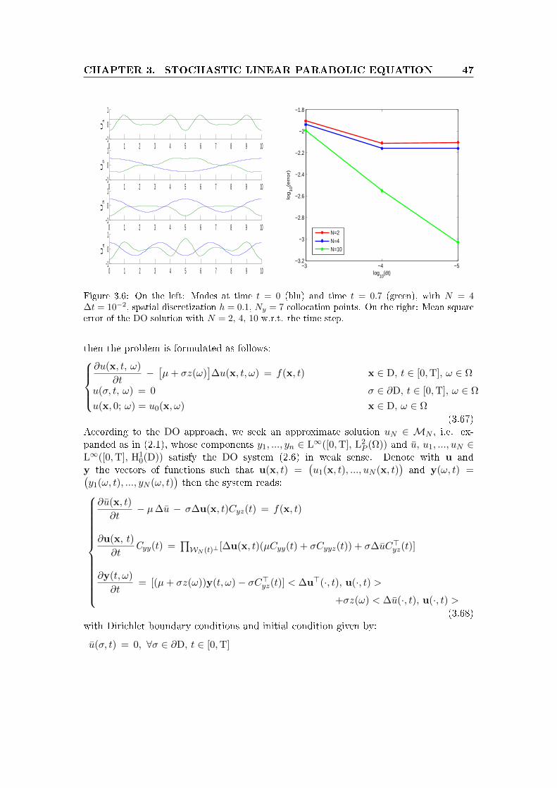
CHAPTER 3. STOCHASTIC LINEAR PARABOLIC EQUATION 47
0 1 2 3 4 5 6 7 8 9 10−1
0
1U
1
0 1 2 3 4 5 6 7 8 9 10−1
0
1
U2
0 1 2 3 4 5 6 7 8 9 10−1
0
1
U3
0 1 2 3 4 5 6 7 8 9 10−1
0
1
U4
−3 −4 −5−3.2
−3
−2.8
−2.6
−2.4
−2.2
−2
−1.8
log10
(dt)
log
10(e
rro
r)
N=2N=4N=10
Figure 3.6: On the left: Modes at time t = 0 (blu) and time t = 0.7 (green), with N = 4∆t = 10−2, spatial discretization h = 0.1, Ny = 7 collocation points. On the right: Mean squareerror of the DO solution with N = 2, 4, 10 w.r.t. the time step.
then the problem is formulated as follows:∂u(x, t, ω)
∂t−[µ+ σz(ω)
]∆u(x, t, ω) = f(x, t) x ∈ D, t ∈ [0,T], ω ∈ Ω
u(σ, t, ω) = 0 σ ∈ ∂D, t ∈ [0,T], ω ∈ Ω
u(x, 0; ω) = u0(x, ω) x ∈ D, ω ∈ Ω
(3.67)According to the DO approach, we seek an approximate solution uN ∈ MN , i.e. ex-panded as in (2.1), whose components y1, ..., yn ∈ L∞([0,T], L2
P (Ω)) and u, u1, ..., uN ∈L∞([0,T], H1
0(D)) satisfy the DO system (2.6) in weak sense. Denote with u andy the vectors of functions such that u(x, t) =
(u1(x, t), ..., uN (x, t)
)and y(ω, t) =(
y1(ω, t), ..., yN (ω, t))then the system reads:
∂u(x, t)
∂t− µ∆u − σ∆u(x, t)Cyz(t) = f(x, t)
∂u(x, t)
∂tCyy(t) =
∏WN (t)⊥ [∆u(x, t)(µCyy(t) + σCyyz(t)) + σ∆uC>yz(t)]
∂y(t, ω)
∂t= [(µ+ σz(ω))y(t, ω)− σC>yz(t)] < ∆u>(·, t), u(·, t) >
+σz(ω) < ∆u(·, t), u(·, t) >(3.68)
with Dirichlet boundary conditions and initial condition given by:
u(σ, t) = 0, ∀σ ∈ ∂D, t ∈ [0,T]

CHAPTER 3. STOCHASTIC LINEAR PARABOLIC EQUATION 48
u(σ, t) = 0 ∀σ ∈ ∂D, t ∈ [0,T]
u0(x) = E[u0(x, ω)] for all x ∈ D,
u0(x) given by the rst N eigenfunctions of the correlation operator Γu(0)u(0),
y0(ω) =< u0(·, ω), u0 > with ω ∈ Ω.
and where we have dened:
• Cyz(t) = E[zy>(t, ·)],
• Cyy(t) = E[y>(t, ·)y(t, ·)],
• Cyyz(t) = E[zy>(t, ·)y(t, ·)]
The weak formulation yields:
. for any t ∈ [0, T], nd u(·, t) ∈ H10(D), u(·, t) ∈ [H1
0(D)]N and y(t, ·) ∈ [L2P (Ω)]N such
that:
<∂u(·, t)∂t
, ψi > +µ < ∇u(·, t), ∇ψi > +σ < ∇u(·, t), ∇ψi > Cyz(t) = f(x, t)
<∂u(·, t)∂t
, ψk > Cyy(t) + p(u(·, t),u(·, t), ψk)[µCyy(t) + σCyyz(t)]
+σp(u(·, t), u(·, t), ψk)C>yz(t) = 0
∂y(t, ω)
∂t− [(µ+ σz(ω))y(t, ω)− σC>yz(t)] < ∇u>(·, t), ∇u(·, t) >
−σz(ω) < ∇u(·, t), ∇u(·, t) >= 0
(3.69)for all ψi, ψk ∈ H1
0(D) and for a.e. ω ∈ Ω; where p(·, ·, ·) is dened as in (3.42).
Similarly to what described in the section 3.2.2, the physical space is discretized withthe Finite Element method, while the stochastic dierential equations are solved by theStochastic Collocation method. The time derivative is discretized by the semi-implicitEuler method and the covariance matrix is treated explicitly in order to decouple theequations dened in the physical domain from those dened in the probability space.Moreover the projection operator is evaluated at the previous time step to recover thelinearity of the problem. Specically, by adopting the same notation as in section 3.2.4,the discretized problem can be written in algebraic form as follows:
MUn+1 + ∆tµKUn+1 + ∆tσKUn+1Cnyz = MUn + ∆tFn
MUn+1Cn + ∆tPnKUn+1(µCn + σCnyyz) + σ∆tPnKUn+1Cnyz = MUnCn
Y n+1 + ∆t(µ+ σZ
)Un+1>KUn+1Y n+1 = Y n
+µ∆tUn+1>KUn+1Cnyz − σ∆tUn+1>KUn+1Z
(3.70)

CHAPTER 3. STOCHASTIC LINEAR PARABOLIC EQUATION 49
where in particular Z is the vector of the values of z in the collocation points, Q is amatrix of dimension N × N dened as Cnyyz = E[(yn)>ynz], Cyz is the column vectorE[(yn)>z] and Pn is the discrete projection operator in the subspace WN (tn), i.e. P =(I−MUn(Un)>).We remark that, contrary to the case in which the diusion term is a deterministicreal value, here the equations for the mean function and the modes are all coupled. Inparticular the equation for the mean led u is coupled to the equations for the otherspatial modes.
0 0.1 0.2 0.3 0.4 0.5 0.6 0.7 0.8 0.90
0.01
0.02
0.03
0.04
0.05
time
Variance
0 0.1 0.2 0.3 0.4 0.5 0.6 0.7 0.8 0.9 10
1
2
3
4
5
6
7
8
time
rank
Figure 3.7: On the left: Numerical test 3.3.1 special initial condition: Time evolution of thevariance of the stochastic coecients with N = 4 ∆t = 10−2, spatial discretization h = 0.1,Ny = 9 collocation points. On the right: Numerical test 3.3.1 general initial condition: Timeevolution of the rank of the covariance matrix associated to the DO solution with N = 2, 4, 8,Ny = 9 collocation points.
3.3.1 Numerical Tests
Special initial condition
Consider the problem governed by the following stochastic PDE:
∂u(x, t;ω)
∂t− β(ω)∆u(x, t;ω) = 0 x ∈ (0, 10), t ∈ T, ω ∈ Ω
u(0, t; ω) = 0 t ∈ T, ω ∈ Ω
u(10, t; ω) = 0 t ∈ T, ω ∈ Ω
u(x, 0; ω) = u0(x) x ∈ (0, 10), ω ∈ Ω
(3.71)where β(ω) is a uniform random variable U(µ, σ2) with µ > 0. Let β(ω) be reformulatedas µ + σz(ω) with z ∼ U [−1, 1]. We consider rst a particular initial condition that is

CHAPTER 3. STOCHASTIC LINEAR PARABOLIC EQUATION 50
1 3 5−4.5
−4
−3.5
−3
−2.5
−2
number of modes
me
an
sq
ua
re
e
rro
r
1.e−1 1.e−2 1.e−3 1.e−4−6
−5
−4
−3
−2
time step
me
an
sq
ua
re
e
rro
r
Figure 3.8: On the left: The mean square error of the DO approximate solution with ∆t = 10−1
(red), ∆t = 10−2 (blu), ∆t = 10−3 (green) Ny = 7 collocation points. On the right: Mean squareerror of the DO approximate solution w.r.t. to the time step, Ny = 7, N = 1.
assumed to coincide with an eigenfunctions of the Laplace operator. Specically it isdened as:
u0(x) =
√1
5sin
(πx
5
)(3.72)
Even if the initial condition is deterministic the solution is immediately aected by thestochasticity of the system at t > 0 and evolves in a 1 dimensional manifold generatedby u0. It reads:
uex(x, t;ω) = e−β(ω)
π2
25t√
1
5sin
(πx
5
)(3.73)
and in particular the exact mean function and the total variance are given by:
uex(x, t) =25
2σ2π2te−(µ+σ2)
π2
25t(eσ2
2π2
25t− 1
)√2
10sin
(2
10πx
)Varex(t) =
25
4σ2π2te−(µ+σ2)
2π2
25t(eσ2
4π2
25t(
1− 25
σ2π2t
)− 1− 25
σ2π2t+
50
σ2π2teσ2
2π2
25t)
(3.74)The analytic solution suggests that the DO method degenerates to the POD method.First of all, according to the DO expansion, the initial datum is reformulated as in (2.1)so that:
• u(x, 0) = u0(x),
• u1(x, 0), ..., uN (x, 0) correspond to the rst N eigenfunctions of the Laplace oper-ator,

CHAPTER 3. STOCHASTIC LINEAR PARABOLIC EQUATION 51
• y1(0, ω), ..., yN (0, ω) are identically equal to zero.
and the DO method leads to a system as in (3.69). Before discussing the numericalresults we observe that the analytical solution in (3.73) can be rewritten as:
uex(x, t;ω) = uex(x, t) + y1(t; ω)u1(x, 0) (3.75)
that leads us to expect only the rst stochastic coecient to evolve. This is conrmedby the numerical results which can be summarized as follows:
• The modes do not evolve. For what concerns the system of PDEs, at each timeiteration only 2 equations are actually solved: the one for the mean function andthe one for the rst mode because this is the only one led associated to a non-zeroeigenvalue.
• All the stochastic evolution is described by the rst random coecient while theothers remain equal to zero, independently of the number of modesN . The varianceof y1, initially zero, grows up as soon as the solution evolves and then it is dissipatedand goes to zero as the solution tends to zero, Figure: 3.7 (left);
• the rank of the covariance matrix is equal to zero at the rst time iteration sincethe initial condition is deterministic and then is steadily equal to one because thesolution is aected by the randomness of the operator as soon as it evolves. Whenthe solution goes to zero all the stochasticity is dissipated, the solution tends to adeterministic function and the covariance matrix returns to be identically equal tozero.
We conclude that the manifold of the solution, which has dimension equal to 1 butthat does not evolve linearly in time (as one can analytically verify in (3.73)), can beapproximated by the rank 1 DO approximate solution, which instead describes a linearmanifold of dimesnion one. Figure 3.8 (left) indeed shows that the error of the DOapproximate solution, in mean square sense, does not depend on the number of modesand the order of convergence is established by the time discretization step size, see Figure3.8 (right).
Special initial condition in a 2D spatial domain
Now we are going to verify if the results of the previous section are inuenced bythe dimension of the physical space. We consider a problem analogous to (3.71) in abi-dimensional spatial domain D = [0, 1]2. Assume that the initial condition is:
u0i(x) =√
2 sin(πx1) sin(πx2)
N∑i=i1,i2
yi0(ω)√
2 sin(i1πx1) sin(i2πx2), (3.76)
where i is a multi-index, N is the number of the deterministic basis functions and allthe stochastic coecients are initialized to zero. Analogously to the mono-dimensional

CHAPTER 3. STOCHASTIC LINEAR PARABOLIC EQUATION 52
0 0.1 0.2 0.3 0.4 0.5 0.6 0.7 0.80
1
2
3
4
5
time
ra
nk
0 0.1 0.2 0.3 0.4 0.5 0.6 0.7 0.8
−15
−10
−5
0
time
va
ria
nce
Figure 3.9: On the left: Time evolution of the rank of the covariance matrix with N = 4,∆t = 10−2, spatial discretization h = 0.05, Ny = 5 collocation points. On the right: Timeevolution of the variance of the stochastic coecient of the DO approximate solution with N = 4,∆t = 10−2, Ny = 5 collocation points (log. scale).
problem, the solution is in a manifold of dimension 1, since only one random variable isinvolved which however is non linear. We computed the DO approximate solution withN between 1,...,10. Figure 3.9 (left) shows that the rank of the covariance matrix inthis case increases in time. On the other hand Figure 3.9 (right) displays that there isa gap between the variance of the random coecients and only one of them developsremarkable variance. This means that the solution can be approximated with only onemode by dropping the stochastic coecients with negligible variance. This is conrmedin Figure 3.10 (left) which shows that the mean square error does not depend on thenumber of modes, or rather the error in the stochastic space is negligible compared to thespatial and temporal discretization error. These considerations concern the approximatesolution computed with 5 collocation points, moreover we aim to verify if this parameterinuences the approximation. Figure 3.10 (right) shows that the error increases whenreducing the number of collocation points and may dominate the time discretization errorfor small ∆t. However it does not change by adding modes, Figure 3.10 (left).
General initial condition
We consider again the problem (3.71) but with a more general initial condition.Specically we chose:
u0(x) =1
100x(x− 10)2 (3.77)
Observe that the initial datum is deterministic but it can not be expressed in terms of anite number of eigenfunctions of the Laplace operator. According to the DO expansion,the initial datum is reformulated as in (2.1) with:

CHAPTER 3. STOCHASTIC LINEAR PARABOLIC EQUATION 53
1 2 3−4.2
−4
−3.8
−3.6
−3.4
−3.2
−3
−2.8
−2.6
−2.4
−2.2
number of modes
me
an
sq
ua
re
e
rro
r
−1 −2 −3 −4
−4
−3
−2
−1
time step
me
an
sq
ua
re
e
rro
r
Figure 3.10: On the left: Error of the DO approximate solution w.r.t the time step and withnumber of collocation points Ny = 2(green), Ny = 3 (red), Ny = 5(green). On the right: Errorof the DO approximate solution with number of collocation points Ny = 3 (red), Ny = 5(green)and with ∆t = 10−1, ∆t = 10−2, ∆t = 10−3.(log-log scale)
• u(x, 0) = u0(x),
• u1(x, 0), ..., uN (x, 0) corresponding to the rst N eigenfunctions of the Laplaceoperator,
• y1(0, ω), ..., yN (0, ω) are identically equal to zero.
and the DO system is dened as in (3.69). In particular the covariance matrix is iden-tically equal to zero at the rst time iteration, being the initial condition deterministic.Contrary to case of deterministic operator and stochastic data analyzed in section 3.2,the stochastic diusion term generates a non linearity in the stochastic space. Becauseof this the solution of (3.71) evolves in a non linear manifold. In addition the manifoldevolves in time, as u is solution of a time-dependent problem. However the dimensionremains equal to 1, since only one random variable is involved in the dierential operatorand no stochasticity comes from the initial datum. The DO approach provides a linearapproximation of the solution in which the eective dimension coincides with the rank ofthe covariance matrix associated to the random coecient. In view of this it is importantto understand how the rank evolves in time with respect to the number of modes andcollocation points, because this tells us the dimension of the linear manifold where thesolution can be approximated. Numerical tests conrm that the rank of the covariancematrix grows up at the second time iteration in order to generate a stochastic subspaceable to describe the process evolution. However we see that the rank remain bounded.It increases up to a maximum values and then it decreases to zero when the solutiongoes asymptotically to the deterministic function zero. The maximum value achievedobviously depends on the number N of basis functions selected initially, as well as on the

CHAPTER 3. STOCHASTIC LINEAR PARABOLIC EQUATION 54
2 4 8−3.3
−3.2
−3.1
−3
−2.9
−2.8
−2.7
−2.6
−2.5
−2.4
number of mdes
ε
1.e−1 1.e−2 1.e−3−2.2
−2
−1.8
−1.6
−1.4
−1.2
time step
me
an
sq
ua
re
e
rro
r
N=1N=3N=5
Figure 3.11: On the left: Approximation error ε(t) of the DO solution with Ny = 9 compared tothe solution of the Stochastic Collocation method with Ny = 20, w.r.t. N, at t = 0.7. ∆t = 10−2,spatial discretization h = 0.1. On the right: Error of the DO solution in mean square sense,w.r.t the time step and with N = 1, 3, 5, Ny = 9 and spatial discretization h = 0.1. (log.scale)
number of collocation points used to solve the stochastic system, specically:
0 ≤ rank(C) ≤ min(N, Ny) (3.78)
As shown in Figure 3.7 (right), in the case we are analyzing the rank reaches the sat-uration level for N = 7. It means that it does not increase any further, even if oneincreases the number of the collocation points and basis functions. This tells us thatthe manifold of the solution, which, we remark, evolves non-linearly in time, can be ap-proximated by 7 modes. They evolve in time by spanning the new directions alongwhich the solution evolves, and no any other mode give contribution to the approxima-tion. We verify the consistency of the analysis concerning the rank of the covariancematrix by computing the error of the DO approximation in the stochastic space. This isestimated by comparing the DO approximate solution to the solution usc of the Stochas-tic Collocation method with highly accurate sparse grid. In Figure 3.11 (left) the errorε(t) = E[‖uN (·, t, ·) − uN (·, t, ·)‖2L(D)] at t = 0.7. The results conrm that no improve-ment are achieved by using N > 4, in accordance with the rank of the covariance matrixat that time step, see Figure 3.7 (right). However it is important to understand how theaccuracy of the approximation degrades if we uses a number of modes N lower than thesaturation level of the covariance matrix. In fact the goal of the DO approach consistsin approximating the solution by using few basis functions possibly and in light of thatwe aim to reduce the dimension of the approximation by dropping out all the compo-nents which do not give remarkable contribution. In Figure (3.11) (left) we compute theapproximation error in norm L2(D) × L2
P (Ω) of the DO solution with dierent numberof modes and with dierent time step. We observe that the error in the stochastic space

CHAPTER 3. STOCHASTIC LINEAR PARABOLIC EQUATION 55
0 0.2 0.4 0.6 0.8 1 1.2 1.4 1.6 1.8 20
0.05
0.1
0.15
0.2
0.25
0.3
0.35
0.4
0.45
time
Total V
ariance
0 0.2 0.4 0.6 0.8 1 1.2 1.4 1.6 1.8 20
0.05
0.1
0.15
0.2
0.25
0.3
0.35
0.4
0.45
time
variance
Figure 3.12: On the left: Time evolution of the total variance of the exact solution. On theright: Time evolution of the variance of the stochastic coecients in the DO expansion for theapproximate solution with N = 4.
dominate the time discretization error with N = 1 and then decreases by adding modesup to the saturation level.
Bi-dimensional stochastic space
We consider now the case in which both the diusion term and the initial conditionare stochastic variables. In particular the problem reads:
∂u(x, t;ω)
∂t− β(ω)∆u(x, t;ω) = 0 x ∈ (0, 10), t ∈ T, ω ∈ Ω
u(0, t; ω) = 0 t ∈ T, ω ∈ Ω
u(10, t; ω) = 0 t ∈ T, ω ∈ Ω
u(x, 0; ω) = u0(x) + z(ω)√
15 sin
(πx5
)x ∈ (0, 10), ω ∈ Ω
(3.79)with u0(x) = 1
100x(x− 10)2 and where z, β are independent uniform random variables,z(ω) ∼ U(µ2, σ
22) and β(ω) ∼ U(µ1, σ
21), with µ1 > 0. Since the random variables
are independent, the stochastic space and consequently the manifold where the solutionlives have dimension 2. The DO approximate solution is then expected to have rank atleast 2. Moreover the manifold of the exact solution is not linear. In Figure 3.14(left) onecan see that the rank of the covariance matrix associated to the DO solution increasesup to 8, when N ≥ 8. We observe that this is an upper bound, which means that therank does not go over 8 independently of N and the number of the collocation points.Furthermore Figure 3.12(right) shows that only few stochastic variables have remarkablevariance, which means that the solution can be approximated in a linear manifold of low

CHAPTER 3. STOCHASTIC LINEAR PARABOLIC EQUATION 56
0 0.02 0.04 0.06 0.08 0.1 0.12 0.14 0.16 0.18 0.2 0.22 0.240
2
4
6
8
10
time
rank
4 6 8 10 12−4.5
−4
−3.5
number of modes
me
an
sq
ua
re
e
rro
rFigure 3.13: On the left: Time evolution of the rank of the DO approximate solution withN = 4, 6, 8, 10 and number of collocation points Ny = 52 (blu) and Ny = 32 (green). Onthe right: Error of the DO approximate solution computed with a number of collocation pointsNy = 52 (blu) and Ny = 32 (green), compared to the solution of the Stochastic Collocationmethod with Ny = 152 in mean square sense.
dimension with good accuracy, as one can see in Figure 3.14(right). The error decreasesaccording to the time step, which implies that the error in the stochastic space is negligiblecompared to the time discretization error for N ≥ 4, in accordance to the time evolutionof the variance of the stochastic variables in Figure 3.12(right).
Reaction term with stochastic coecient
We conclude this section with a more challenging example in which both the coe-cients of the diusion and reaction terms are stochastic variables:
∂u(x, t; ω)
∂t− β(ω)∆u(x, t; ω) = δ(ω)F (u(x, t;ω)) x ∈ (0, 10), t ∈ T, ω ∈ Ω
∂u
∂x(0, t; ω) = 0 t ∈ T, ω ∈ Ω
∂u
∂x(10, t; ω) = 0 t ∈ T, ω ∈ Ω
u(x, 0; ω) =
1 x ≤ 5
0 x > 5ω ∈ Ω
(3.80)where F (u) = u(u−1)(α−u) with α ∈ (0, 1), β(ω) and δ(ω) are two uniform independentrandom variables. The solution is then described by a bi-dimensional manifold that isstrongly not linearly, since the reaction term is a cubic polynomial. In the previous exam-ple we have seen that by increasing the number of modes, and equivalently the dimensionof the linear manifold where we approximate the solution, we can improve the accuracy

CHAPTER 3. STOCHASTIC LINEAR PARABOLIC EQUATION 57
0 0.1 0.2 0.3 0.4 0.5 0.6 0.7 0.81
2
3
4
5
6
7
8
9
time
ra
nk
1.e−1 1.e−2 1.e−3
−3.8
−3.4
−3
−2.6
−2.2
−1.8−1.8
time step
me
an
sq
ua
re
e
rro
r
Figure 3.14: On the left: Time evolution of the rank of the DO approximate solution withN = 4, 8, 12, ∆t = 10−3, number of collocation points Ny = 15 . On the right: Error of the DOapproximate solution in mean square sense, w.r.t the time step and with N = 4, 5, number ofcollocation points Ny = 52
of the approximation, up to the saturation level of the covariance matrix. However thenumber of collocation points represents an other important parameter that inuencesthe approximation, since the stochastic coecients and, consequently the approximatesolution, are approximated in a polynomial space using the evaluations in the collocationpoints. Figure 3.13(left) shows that the increasing trend of the rank of the covariancematrix is indeed inuenced by the number of collocation points, and consequently alsothe accuracy of the approximate solution. We compared the solution of the DO andStochastic Collocation method, this one computed with a highly accurate sparse grid, inorder to quantify the inuence of this parameter. Figure 3.13(right) shoes the error, inmean square sense, of two DO approximate solutions, computed with a stochastic tensorgrid with respectively 3 and 5 collocation point per axis, compared to the solution ofthe Stochastic Collocation method that uses 15 points. One can see that the error ofthe DO approximate solution decreases by using a more accurate stochastic grid. Thiscan be explained by reminding that the DO approximate solution tends to coincide tothe solution of the Stochastic Collocation method by increasing N up to the number ofcollocation points. Then with a large number of modes the convergence rate depends onthe number of collocation points in the same way as that of the Stochastic Collocationmethod.

Chapter 4
Stochastic Reaction-Diusion
Equations: application to the
electrocardiology
In this chapter we focus on parabolic dierential equations with non linear reactionterm describing the electric signal in biological tissues. After discussing the probabilisticapproach, we are going to verify the eectiveness of the DO method to this type ofequations.
4.1 Cardiac Electrical Activity and Mathematical Models
The heart is a muscular organ that acts as a pump. The ow of ions across the cellmembranes causes electrical impulses that give rise to perpetuating waves of excitation.The wave spreads through the whole heart and enables the impulse to travel from a cellto another. This excitation state and its spread is what coordinates and feeds the con-tractions of the cardiac cells. From a macroscopic point of view, this is essentially whathappens when blood is pumped to the body. However this process depends on severalparameters and it is correlated to many other sub-process. This makes the problem quitecomplex to modelize.Cardiac cells have two features linked each other: they have a contractile ability andthey are excitable. The action of the mechanical function is caused by electrical signalsthat propagate in the tissue while the propagation is allowed by the excitability of thecells. The stimulation arises in the sinoatrial node where the pacemecker cells generatethe electric pulse that determines the heart beat. When an excitable cell is activatedthe membrane potential of that cell generates the so-called action potential . It is causedby a potential dierence that gives rise to transfer of ionic charges. When the localdepolarization reaches a certain threshold the action potential starts and the impulse istransmitted to neighboring cells. For details [29].The Hodgkin Huxley and subsequently many other models have been developed to de-

CHAPTER 4. STOCHASTIC REACTION-DIFFUSION EQUATIONS:
APPLICATION TO THE ELECTROCARDIOLOGY 59
scribe the action potential of a single cell. They consist on biophysically-based modeland reproduce the action potential by modeling the underlying sub-cellular processes.An alternative to this complex approach is provided by non-biophysical models, amongwhich the most known is probably the FitzHugh-Nagumo one. These simplied modelsaim at describing the qualitative features of the action potential without attemptingto address the underlying bio-physiological processes. For details [28].
4.2 Traveling waves
A traveling wave is a solution that travels at constant speed with xed shape. Werecall two types of traveling waves in excitable systems. The rst one, called travelingfront, is characterized by two steady levels: some low value in front of the wave and somehigher value behind the wave. On the contrary, the other one can be described as a curvethat begins and end at the same value. It means that a recovery phase, which followsthe excitation, takes the wave back to the initial state. This is called traveling pulse.In other words a traveling front acts like a zipper switching from resting to excitingstate. If the recovery variable can force back the solution to the steady state we have thetraveling pulse.We focus on the traveling front without considering the recovery variable, or equivalentlyby assuming it xed to the steady state. The evolution of a traveling front is describedby the bistable equation, so called because it has two stable rest points. It is related tothe FitzHugh−Nagumo model, without recovery, described in the next section.
4.2.1 Travelling fronts: Bistable equation
The Bistable equation is a spacial case of Cable equation and it consists in a parabolicPDE, with non linear reaction term, i.e.:
∂u
∂t−∆u = f(u) (4.1)
where f(u) is assumed to be a cubic polynomial. We assume f(u) having the zeros at0, 1 and α, with α ∈ (0, 1). The rst two zeros are stable which means that u = 0 andu = 1 are the steady equilibriums of the PDE. The other zero α is instead repulsive. Thedynamics of the solution is described by the transition between the two steady states.This feature makes u a travelling front. The reaction term can be written in the followingform:
f(u) = Au(u− 1)(α− u) α ∈ (0, 1) (4.2)
where A is a constant that determines the speed of the wave.We have seen that the excitable dynamics comes from the reaction term and in particularfor large A the reaction dominates the diusion. This generates dynamics characterizedby sharp fronts.Analytic solution can be obtained only for particular initial conditions. This makesthe wave propagation in the FitzHugh − Nagumo model not completely understood

CHAPTER 4. STOCHASTIC REACTION-DIFFUSION EQUATIONS:
APPLICATION TO THE ELECTROCARDIOLOGY 60
yet, especially with multidimensional spatial domain. On the other hand the numericalapproach can achieve good results even if small discretization time step and specicnumerical treatment are often required to handle with the reaction term which, besidegenerating sharp slops and fast dynamics, is not linear.We start the analysis from the mono-dimensional case for which an analytic solution canbe derived. This enables us to understand how the parameters inuence the dynamicand which implications we should expect by considering them as stochastic variables.Furthermore it give us the opportunity to test the quality of the numerical results.Let us consider the problem in a mono-dimensional domain:
∂u
∂t− ∂2u
∂x2= f(u) (4.3)
Since the traveling front is a wave that travels with constant speed c, we seek a solutionof the form:
u(x, t) = v(x+ ct) (4.4)
Denoting with ξ the new variable ξ = x+ ct, the PDE 4.3 becomes:
cv′′ − v′ = f(v) (4.5)
After solving the previous ordinary dierential equation, for details ( [29]), we conclude
that the problem 4.3 with initial condition u(x, 0) = 12 + 1
2 tanh(√A
2√
2x)have the following
analytic solution:
u(x, t) =1
2+
1
2tanh
(√A
2√
2(x+ ct)
)(4.6)
where the speed c is given by:
c =
√A
2(1− 2α) (4.7)
Observe that the speed of the propagation depends on α, that is the repulsive zero ofthe reaction function f(u). In particular the speed decreases as α tends to 0.5, value forwhich the direction of the wave propagation changes.
Stochastic approach
From a biological point of view the PDE in (4.1) models the ionic current through thecellular membranes and the inter-cellular space and provides a macroscopic descriptionof the action potential avoiding to directly involve the related sub-cellular processes. Itrepresents an alternative to the biophysically based models which detail several cellularinteractions by adding more and more functions. The constant A represents the exci-tation rate and α is the normalized threshold potential value. They depend on severalvariables among which the membrane capacitance, the membrane resistance, cytoplasmicresistance, cell diameter and clearly the ionic channel conductances. All these parameters
CHAPTER 4. STOCHASTIC REACTION-DIFFUSION EQUATIONS:
APPLICATION TO THE ELECTROCARDIOLOGY 61
are largely uncertain and such uncertainty should be properly included in the determin-istic model. The tting of parameters requires sophisticated anatomical, physiological,biological and clinical experimental programs that not only are dicult to achieve butare also very prone to noises. In addition the parameters depend on each individualand they may change in time, as consequence of many situations among which diseases,stress, diet and so on. By considering stochastic parameters we can achieve comprehen-sive analysis which incorporate the uncertainty that is intrinsically part of the problemas well that which comes from the measurement.For what concerns the bistable equation, the problem can be formulated as follows:
∂u
∂t−∆u = A(ω)u(u− 1)(α(ω)− u)
u|t0 = u0(x, ω)(4.8)
where the solution u(x, t, ω) is a stochastic process and the parameters, the initial con-dition or both of them are stochastic.
4.3 Bistable Equation: DO approach
In this section we apply the DO approach to the stochastic bistable equation. Afterprovided the DO formulation of the problem and the computational details, we discuss thenumerical results by distinguish two typologies of problem: in the rst the stochasticity isintrinsically part of the operator in the governing equations, in the second the randomnessis totally generated by the initial condition. We aim to investigate if and in which casesthe low rank approximation is a suitable approach to approximate excitable systems asin (4.8), and how the source of uncertainty aects the answer.
4.3.1 DO formulation
We consider the stochastic problem governed by SPDE in (4.8) with Neumannboundary conditions. We remind that the DO approach computes an approximate solu-tion inMN , the subspace of all the N rank stochastic elds, by projecting at each timeinstant the residual of the equation (4.8) onto Tu(t)MN that is the tangent space toMN
at uN (t). In the specic case of the stochastic bistable equation the DO method resultsin solving the following system:
∂u(x, t)
∂t− ∆u(x, t) = E[f(u(x, t;ω); ω)] x ∈ D, t ∈ [0,T], ω ∈ Ω
∑Ni=1
∂ui(x, t)
∂tCyiyj (t) =
∏W⊥N
∑Nk=1
[∆uk(x, t)Cykyj (t) + E[f(u(x, t;ω); ω)yj(t; ω)]
],
∀ j = 1, ...Ndyi(t, ω)
dt=<
∑Nk=1 ∆uk(x, t)yk(t, ω) + f(u(x, t;ω);ω)− E[f(u(x, t;ω); ω)], ui(x, t) >
∀ i = 1, ..., N
(4.9)

CHAPTER 4. STOCHASTIC REACTION-DIFFUSION EQUATIONS:
APPLICATION TO THE ELECTROCARDIOLOGY 62
with the following boundary conditions:
∂u
∂n(σ, t) = 0 σ ∈ ∂D, t ∈ [0,T]
∂ui∂n
(σ, t) = 0 ∀i = 1, ..., N
where n denotes the normal to the boundary ∂D, and with initial conditions given by:
• u0(x) = E[u0(x, ω)] for all x ∈ D,
• u0i(x)i=1,...N that are the rst N eigenfunctions of the correlation operatorCu(0)u(0),
• yi0(ω) =< u0(·, ω), u0i > with ω ∈ Ω and for any i = 1, ...N .
System (4.9) consists in N + 1 deterministic PDEs coupled to N stochastic ODEs andthe approximate solution is recovered as:
uN (x, t; ω) = u(x, t) +
N∑i=1
yi(t; ω)ui(x, t) (4.10)
being N the dimension of the manifold in which the solution u of (4.8) is approximated.We assume u, u1, ..., uN ∈ L∞([0, T], H1(D) and y1, ..., yN ∈ L∞([0, T], L2
P (Ω). Denotedwith u and y the vector of functions such that u(x, t) =
(u1(x, t), ..., uN (x, t)
)and
y(ω, t) =(y1(ω, t), ..., yN (ω, t)
)the weak formulation of (4.9) reads: for any t ∈ [0, T],
nd u(·, t) ∈ H1(D), u(·, t) ∈ [H1(D)]N and y(t, ·) ∈ [L2(Ω)]N such that:
<∂u(·, t)∂t
, ψ > + < ∇u(·, t), ∇ψ >=< E[f(u(·, t, ·))], ψ >
<∂u(·, t)∂t
, ψ > C (t) + p1(u(·, t),u(·, t), ψ)C (t) = p2(u(·, t),E[f(u(·, t, ·))>y], ψ)
∂y(t, ω)
∂t+ y(t, ω) < ∇u(·, t), ∇u(·, t) >=< f(u(·, t, ·))− E[f(u(·, t, ·))], u(·, t) >
(4.11)for all ψ ∈ H1(D) and where p1(·, ·, ·), p2(·, ·, ·) is dened as:
p1 : (u,v, w)→ − < Π<u>>∆v, w >
p1(u,v, w) =< ∇v, ∇w > − < w, u >< ∇v,∇u >(4.12)
for any u, v, w ∈ [H1(Ω)]N and < ui, uj >= δij .
p2 : (u,v, w)→ < Π<u>>v, w >
p2(u,v, w) =< v, w > − < w, u >< v,u >(4.13)

CHAPTER 4. STOCHASTIC REACTION-DIFFUSION EQUATIONS:
APPLICATION TO THE ELECTROCARDIOLOGY 63
for any u, v, w ∈ [L2(Ω)]N and < ui, uj >= δij . Even if at the continuous level allthe equations in (4DOeq) are coupled each other, they can be divided in two subsystem,one deterministic and one stochastic and two independent discretization strategies canbe adopted in the physical and probability space.
4.3.2 Numerical Approximation
Similarly to what described in Section 3.2.2 the deterministic PDEs are solved byusing the Galerkin method with linear nite element discretization while the Stochas-tic Collocation method is used to solve the stochastic ODEs. According to the weakformulation (4.10) at any t the basis functions are discretized in the nite dimensionalspace Wh ⊂ H1(D) of continuous piecewise linear functions dened in the triangula-tion Th of the physical domain. The stochastic coecients are instead computed as aglobal polynomial approximation upon the solutions obtained by collocating the govern-ing equations in each collocation point. The details of the two method are described inthe section 3.2.2. The time derivative is discretized with the Euler method. In particularthe diusion terms are always treat implicitly while the reaction term, that is non linear,explicitly. Once again the covariance matrix C(t) is freezed at the previous time stepwhen solving the deterministic equations, the same applies to the projection operator.All these choices are motived by the purpose of keeping the deterministic equations de-coupled from the stochastic equations in order to take the computational cost of theDO method low. A fully coupled system for problems as in (4.10) indeed require a highcomputational eort. By using the same notation introduced in the Chapter 3, we passdirectly to the algebraic form of (4.10):
MUn+1 + ∆tKUn+1 = MUn + ∆tMFn
MUn+1Cn + ∆t(I −MUnUn>)KUn+1Cn = MUnCn + ∆t(I−MUnUn>)MFYn
Y n+1 + ∆tUn+1>KUn+1Y n+1 = Y n + ∆tUn+1>M(Fn − Fn
)(4.14)
where F is the column vector of the nodal values of E[f(u)] at time tn, i.e. Fn = E[f(uh)]and F ∈ RNh×Ny and FY n
i j = RNh×N are the matrices dened as Fni j = f(uh(xi, tn, ξj))
and FYni j = E[f(uh(xi, t
n, ·)yj(tn, ·)] respectively. The symbol E[·] denotes the ap-proximated expected value estimated through quadrature formula corresponding to thecollocation points.We observe that the equation for the mean function is decoupled from the others. Onthe contrary the second set of equations are coupled each other through the covariancematrix that is possibly singular and then not invertible. The strategy we adopted toovercome the problem consists in diagonalizing the covariance matrix. In other wordsthe expansion in (4.10) is re-orthogonalized in L2(Ω) before solving the PDEs for thedeterministic basis functions. By denition the covariance matrix is symmetric andpositive semi-denite. It follows that at any time instant there exists a set of N eigenval-

CHAPTER 4. STOCHASTIC REACTION-DIFFUSION EQUATIONS:
APPLICATION TO THE ELECTROCARDIOLOGY 64
ues λk(t)Nk=1 and N eigenvector vk(t)Nk=1 orthogonal with respect to the euclideannorm.Therefore at any time instant there exists a transformation according to which thestochastic eld uN ∈ MN can be expanded in orthogonal basis on the stochastic space,i.e.:
uN (x, t; ω) = u(x, t) +N∑i=1
zi(t; ω)wi(x, t) (4.15)
with:
• wj(x, t) =∑N
i=1 uj(x, t)vi j(t)
• zj(t; ω) =∑N
i=1 yi(t; ω)vj i(t)
In particular the covariance matrix associated to the stochastic coecients in (4.30)corresponds to the diagonal matrix of the eigenvalues of C. However we stress that theorthogonality of the random variables is not required by the DO approach and aboveall it is not preserved in time. Indeed the approximation of the initial datum, accordingto the KL expansion, provides a double orthogonal decomposition, but that feature isnot preserved except in the case in which the principal components of u0 coincide withthe eigenvalues of the operator L. At each time iteration we diagonalize the covariancematrix and we solve the deterministic system of PDEs in to the unknowns w1, ..., wN ,by considering the eigenvectors v1, ..., vN freezed at the previous time step. Specically,dened V and D the matrices of eigenvectors and eigenvalues of C, it holds:
MUn+1VnDn + ∆t(I −MUnUn>)KUn+1VnDn= MUnVnDn + ∆t(I−MUnUn>)ME[FnY n>Vn]
(4.16)By assuming the eigenvectors xed in time at each iteration, (4.16) can be written interms of the alternative orthogonal representation as:
MWn+1Dn + ∆t(I −MUnUn>)KWn+1Dn= MWnDn + ∆t(I−MUnUn>)ME[FnZn>]
(4.17)
where W ∗ = U∗Vn and Zn = Vn>Y n.Now, in view of the proposition (2.6.1) the deterministic elds associated to zero variancestochastic coecients are left unchanged. Observe that this treatment is consistent withthe problem because on the right side we recover E[FnZn>], i.e. the correlation betweenthe reaction term and the uncorrelated stochastic variables, both of them treated explic-itly. In particular the correlation is null when the stochastic variable has zero variance.

CHAPTER 4. STOCHASTIC REACTION-DIFFUSION EQUATIONS:
APPLICATION TO THE ELECTROCARDIOLOGY 65
In conclusion the DO system reads:
MUn+1 + ∆tKUn+1 = MUn + ∆tMFn
MWn+1i + ∆t(I −MUnUn>)KWn+1
i = M Wni +
1
λi∆t(I−MUnUn>)ME[FnZn>i ]
if λni > 0
Un+1i = Uni
ifλni < 0Y n+1 + ∆tUn+1>KUn+1Y n+1 = Y n + ∆tUn+1>KUn+1
(Fn − Fn
)(4.18)
4.3.3 Implementation details
The DO approach explicitly requires to the deterministic basis functions to be or-thonormal in L2(D). Can be easily veried that the condition is preserved at the contin-uous level. On the other hand this is not guaranteed from a numerical point of view. Theproblems analyzed in this section are characterized by fast dynamics that consequentlyaects the covariance matrix and its eigenvalues. In order to overcome the problem wechose to re-orthonormalize the deterministic basis functions at each time iteration, oncesolved the system (4.16). The procedure adopted is analogous to what described in thesubsection 3.2.5. We underline that the deterministic basis functions are orthogonalizedbefore solving the equations for the stochastic coecients, since we adopt a Gauss Seideltype approach. This constraint explicitly imposed at each time step as well the diago-nalization of the equations for the deterministic basis functions, nalized in particularto deal with singular covariance matrix, justies our choice in the time discretization ofusing a 1 step method instead of a multi step one. Possible numerical scheme to preservethe orthogonality are proposed in [36].
4.4 Bistable equation with stochastic threshold potential
In this section we consider a mono-domain formulation of the bistable equation, wherethe spatial domain is assumed to coincide with one myocardial cell with no connectionbetween the intracellular domain and any surrounding media. From the mathematicalpoint of view this means that we impose homogeneous boundary conditions type Neu-mann on the surface of cell to prevent current ow out the domain. We analyze thecase in which the threshold potential is assumed to be a stochastic variable and theproblem is modeled by a time dependent stochastic PDE, corresponding to the bistableequation, with deterministic initial conditions. Say the reaction term a cubic polynomialf(u, ω) = Au(α(ω) − u)(u − 1) and α(ω), the instable zero of f , a stochastic variable,the problem reads:
∂u(x, t, ω)
∂t−∆u(x, t, ω) = f(u(x, t, ω), ω) x ∈ D, t ∈ [0, T], ω ∈ Ω
u(x, 0, ω) = u0(x)∂u
∂n(σ, t, ω) = 0 σ ∈ ∂D
(4.19)

CHAPTER 4. STOCHASTIC REACTION-DIFFUSION EQUATIONS:
APPLICATION TO THE ELECTROCARDIOLOGY 66
where n is is the unit normal vector to the boundary. In order to understand how thestochasticity of the parameter α inuences the system, we focus rst on the the mono-dimensional problem mentioned in section 4.2.1, for which we recovered an analyticsolution. Then we discuss the numerical results of the DO method, applied to problem(4.20). We start by describing the qualitative features and then we analyze the accuracyof the DO approximate solution, compared to the one of the Stochastic Collocationmethod and the best N rank approximation.
4.4.1 Modeling problem
We start by considering the mono-dimensional problem:∂u(x, t, ω)
∂t− ∂2u(x, t, ω)
∂2x= f(u(x, t, ω), ω) x ∈ (−∞, ∞), t ∈ [0, T], ω ∈ Ω
u(x, 0, ω) = 12 + 1
2 tanh(√A
2√
2x)
(4.20)where the reaction function is a stochastic eld dened as f(u(x, t; ω), ω) = Au(α(ω)−u)(u− 1). The excitation rate A and the initial datum are assumed to be deterministicand the stochasticity of the system is uniquely generated by the random variable α. Inparticular we suppose α(ω) ∈ L∞(Ω) and bounded between 0 and 1. According to (4.7)the propagation speed of the traveling front depends on the threshold potential value αand then it is as well a random variable:
c ∈ L∞P (Ω) s. t. c(ω) =
√A
2(1− 2α(ω)) (4.21)
Similarly to the deterministic case, the analytic solution of problem (4.20) is given by:
u(x, t; ω) =1
2+
1
2tanh
(√A
2√
2(x+c(ω)t)
)x ∈ (−∞, ∞), t ∈ [0, T], ω ∈ Ω (4.22)
and it is a traveling front with random propagation speed. Since the range of the pa-rameter α has to be bounded between zero and one, we choose to model it as a uniformrandom variable. We observe that α = 0.5 is a critic point since it is the values forwhich the direction of the front changes. For values of α bigger than 0.5 the solutionconverges to the steady state u = 0 while for outcomes smaller than 0.5 it tends to thehigher steady level. The value α = 0.5 is instead a point of zero probability for which thesolution doesn't evolve. It means that if we consider the sign of c(ω) as function denedin the stochastic space, then α = 0.5 is a discontinuity point. In particular it representsa discontinuity point in the stochastic space for the solution u at t that tends to innity.In fact for vales of α lower that 0.5, u tends asymptotically to the higher steady equilib-rium u = 1, otherwise it tends to 0. In view of applying the DO approach, we remindthat the Stochastic Collocation method is often not suitable to describe discontinuousrandom elds. A good possibility to overcame the problem consists on decomposing the

CHAPTER 4. STOCHASTIC REACTION-DIFFUSION EQUATIONS:
APPLICATION TO THE ELECTROCARDIOLOGY 67
stochastic domain in the two intervals where the solution is continuous and then sepa-rately solve the equations for each interval.We describe here only the case in which all the possible outcomes of α are smaller then0.5, the opposite case gives the same results for what concerns our purposes. Specicallywe consider α(ω) = 0.2(1 + z(ω)) where z is an uniform random variable in [−1, 1].For computational reason we need to consider a nite physical domain. We observe thatfor xed t it holds:
limx→∞
u(x, t, ω) = 1 limx→−∞
u(x, t, ω) = 0 ∀ω ∈ Ω (4.23)
Moreover for big values of A the solution u(x, t, ω) is characterized by a sharp frontdened in a small spatial interval, outside of which the function approaches rapidly thesteady states zero or one. We analyze therefore the problem (4.20) from the compu-tational point of view by considering Neumann homogeneous boundary conditions in anite interval [−d, d] with d > 0. Specically the problem reads:
∂u(x, t, ω)
∂t− ∂2u(x, t, ω)
∂2x= f(u(x, t, ω), ω) x ∈ (−d, d), t ∈ [0, T], ω ∈ Ω
∂u
∂x(d, t, ω) = 0
∂u
∂x(−d, t, ω) = 0
u(x, 0; ω) = 12 + 1
2 tanh(√A
2√
2x)
x ∈ [−d, d], ω ∈ Ω
(4.24)that is consistent with the original problem, as the wave travels within the interval. Wewill use this result to verify the accuracy of the DO approximate solution in section 4.4.2
4.4.2 Numerical Results
Initialization of the deterministic basis functions
In order to apply the DO method the initial condition has to be expanded as in(4.10). For stochastic initial condition the initial datum is expanded by following theKL decomposition and approximated in MN by the eigenfunctions of the correlationoperator which are associated to larger variance. The deterministic basis function arethen initialized to the rstN principal components of the initial datum. For deterministicinitial condition instead it is necessary to adopt an other dierent strategy since the initialfunction does not have any component in the stochastic space and a priori there is notany privileged direction. However for consistence with the problem, at time t = 0 themean value has to coincide with the deterministic initial datum while the stochasticcoecients have to be initialized to zero. We observe that the term
N∑i=1
yi(t, ω)ui(x, t)

CHAPTER 4. STOCHASTIC REACTION-DIFFUSION EQUATIONS:
APPLICATION TO THE ELECTROCARDIOLOGY 68
does not give any contribution at the t = 0 since the stochastic coecients are identi-cally equal to zero. Then the deterministic basis u1, ..., uN can be chosen to correspondto any sequence of N orthonormal functions in L2(D). Given the homogeneous Neumannboundary conditions, one possibility consists in using cosine functions.We call latent a basis function associated to a stochastic coecient with zero variancewhile we say that a basis function is activate when the associated random variable de-velops variance larger than zero. At xed time t, only the activate variables inuencethe approximation of the solution. They evolve in time to adapt to the structure of theproblem while the other are left unchanged. However the adaptation of the basis func-tions is subjected to the error due to the time discretization. In particular the evolutionof the modes, determined by the equations in (4.18), depends on the eigenvalues of thecovariance matrix that is treated explicitly as well as the projection operator. Howevernumerical tests conrm that the error in the adaptation of the modes decreases accordingto the time step and it is negligible compared to the approximation error in the stochasticspace for small N . Another practical option to initialize the terms of the DO expansion(4.10) consists in adding additional variance to the initial datum. We observe that at therst iteration the modes do not evolve since the covariance matrix is identically equal tozero. By introducing an additional variance, that is small enough to generate a negligibleerror, we can overcome the problem. From the computational point of view, say ρ thethreshold over which the variance of the stochastic variables is considered not zero, oneor more stochastic coecients are initialized to an arbitrary random variable with orderof magnitude equal to ρ. In what follows we adopted the rst approach.
Qualitative analysis
Before going into details about the accuracy of the DO approximation we give anexample that highlights the mean features of the method.The DO approximate solution consists in a linear combination of deterministic modesand stochastic coecients. Unlike the classical spectral approaches introduced in section1.3, nor polynomial or any xed structures are imposed a priori. Both the modes andthe stochastic coecients are computed on y, that means at each time iteration, inorder to capture the structure of the problem. In this way few modes aim at globallyapproximate the main feature of the solution. In addiction, the DO expansion is asuitable representation of stochastic elds for what concerns the numerical UncertaintyQuantication, context in which the goal is usually to compute statistics of the solution,in particular mean and variance. By following the DO approach the mean eld is treatedseparately from the other modes and it is directly calculated by the method at each timestep. The linear combination of the modes, with the stochastic coecients, describesinstead the variability of the process in the stochastic space and in particular the sumof the variance of the single stochastic variables corresponds to the total variance of theapproximate solution. In this way we actually have a comprehensive description of thesolution, as it is emphasized by the numerical test which we are going to describe.

CHAPTER 4. STOCHASTIC REACTION-DIFFUSION EQUATIONS:
APPLICATION TO THE ELECTROCARDIOLOGY 69
0
1 0
1
0
1
0
0.1
0.2
0.3
0.4
0.5
0.6
0.7
0.8
0.9
1
0
1 00.2
0.40.6
0.81
−0.2
0
0.2
−0.1
−0.05
0
0.05
0.1
0
1 0
1
−4
0
4
−3
−2
−1
0
1
2
3
Figure 4.1: The mean eld at t = 0.05 (left) and the standard deviation at time at t = 0.05(middle) and at t = 0.5 (right) of the solution computed with the Stochastic Collocation methodwith highly accurate sparse grid.
Consider the stochastic dynamical system governed by the following SPDE:
∂u(x, t, ω)
∂t− δ∆u(x, t, ω) = f(u(x, t, ω)) x ∈ D = [0, 1]2, t ∈ [0, T], ω ∈ Ω
∂u
∂n(σ, t, ω) = 0 σ ∈ ∂D
u(x, 0; ω) =
1 if x1 ≤ 0.5
0 if x1 > 0.5
(4.25)where f(u) = 100u(u − 1)(α(ω) − u), α(ω) is an uniform random variable with meanµ = 0.2 and variance σ2 = 0.013 and the diusion coecient is δ = 0.01. The solution isa stochastic eld which tends asymptotically to the deterministic function u = 1 as t goesto innity and it consists in a sheaf of traveling fronts with stochastic propagation speedin (4.21). Figure 4.1 shows the mean eld (left) and the standard deviation (right) ofthe numerical solution computed with the Stochastic Collocation method with a highlyaccurate sparse grid. The DO solution can be computed as described in section 4.3.1.The initial mean function corresponds to the initial datum which is deterministic andthe modes are arbitrarily initialized to a sequence of N orthonormal basis functions in[0, 1]2 with zero stochastic coecients. In this example we choose the cosine functions:ui(x1, x2) =
√2 cos(iπx1)cos(jπx2), for i, j = 1, ...,
√N . Figure 4.2 shows that the
mean functions is a traveling front that actually describes the propagation of the solution.Moreover the modes evolve in time and properly adapt to describe the variability of thepropagation speed. We observe that at any time instant the physical domain can bedivided in three parts and we describe each of them by qualitatively comparing theexact solution, or rather the reference solution computed with the Stochastic Collocationmethod with a highly accurate sparse grid, and the DO approximate solution. Figure4.2 shows the mean function and while in Figure 4.4 we present the rst two modes ofthe DO approximate solution at dierent time steps.
• Part 1: the solution is already at the higher equilibrium level, u = 1. Here u isequal to a deterministic value for almost all ω ∈ Ω and then the variance eld is

CHAPTER 4. STOCHASTIC REACTION-DIFFUSION EQUATIONS:
APPLICATION TO THE ELECTROCARDIOLOGY 70
0
1 0
1
0
1
0
1 0
1
0
1
0
1 0
1
0
1
Figure 4.2: Mean function of the DO approximate solution at t = 0 (left), t = 0.05 (middle) andt = 0.5 (right), with N = 6, Ny = 7, ∆t = 0.001
equal to 0, as shown in (4.1). In accordance with this fact, all the activated modesare equal to zero. We recall that at the xed time t only the modes associated tostochastic coecients with variance larger than zero evolve, the other ones are leftunchanged and do not give any contribution to the solution at t (however theymight evolve at t > t). The mean function of DO approximate solution is properlyequal to 1 and it is the only one term that gives remarkable contribution to theapproximation.
• Part 2: the portion of the domain that corresponds to the curve of the stochastictraveling front. Here the stochasticity of the process is concentrated, the stan-dard deviation is dierent from zero and the mean function represents the meanshape. The DO approximate solution is able to describe both the mean eld andits variability; the mean function is close to the exact one and the activate modes,especially the ones that are associated to stochastic variables with large variance,adapt to the same shape of standard deviation.
• Part 3: the portion of the domain which has not yet been reached by the travelingfront. The solution here is equal to the deterministic function u = 0 and boththe standard deviation and the activate modes are constantly equal to zero. Themean function is zero as well and coincides with the exact one.
The same observation can be done at each time step, and this shows that the DO ap-proximate solution is consistent with the qualitative features of the exact solution. Themodes, which promptly adapt since the rst time step, evolve in time by following thetraveling front as well as the mean function. This shows that the DO method actuallycaptures the structure of the process without any a priori information and properlydescribes the qualitative features of both the mean and the standard deviation eld.
A posteriori estimates
In order to understand the dynamics of the solution in the stochastic space and thesuitability of the low rank approach, we analyze the evolution in time of the covariance

CHAPTER 4. STOCHASTIC REACTION-DIFFUSION EQUATIONS:
APPLICATION TO THE ELECTROCARDIOLOGY 71
0
1 0
1
−6
0
4
−2
−1.5
−1
−0.5
0
0.5
1
1.5
2
0
1 0
1
−6
0
4
−5
−4
−3
−2
−1
0
0
1 0
1
−6
0
4
−3
−2.5
−2
−1.5
−1
−0.5
0
0.5
1
Figure 4.3: First mode of the DO approximate solution at t = 0 (left), t = 0.05 (middle) andt = 0.5 (right), with N = 6, Ny = 7, ∆t = 0.001
0
1 0
1
−6
0
4
−2
−1.5
−1
−0.5
0
0.5
1
1.5
2
0
1 0
1
−6
0
4
−5
−4
−3
−2
−1
0
1
2
3
0
1 0
1
−6
0
4
−2
−1.5
−1
−0.5
0
0.5
1
1.5
2
2.5
3
Figure 4.4: Second mode of the DO approximate solution at t = 0 (left) t = 0.05 (middle) andt = 0.5 (right), with N = 6, Ny = 7, ∆t = 0.001,
matrix and in particular the rank, which corresponds to the eective rank of the approx-imate solution, and the eigenvalues, for dierent values of N .Let us consider problem (4.24), the stochastic space has dimension equal to one since thestochasticity is uniquely determined by the random variable α. Thus the exact solutionevolves in a one-dimensional manifold, which however is non linear, as shown by theanalytic solution in (4.22). The traveling front is deterministic at t = 0, it propagateswith the stochastic speed in (4.21) and then tends asymptotically to the deterministicvalue that corresponds to the steady equilibrium (in this case u = 1). Consequently, weexpect that the rank of the covariance matrix, initially equal to zero, would increase andthen go back to zero. It easy to verify that, at any time instant, the total variance of theapproximate solution corresponds to the sum of the variance of the stochastic coecients,or equivalently to the sum of the eigenvalues of C(t).
Var[‖uN (·, t, ·)‖L2(D)] =
N∑i=1
Var[yi(t, ·)] =
N∑i=1
λi(t)
Concerning the covariance matrix, the dynamic of the rank depends on both the num-ber of modes and the number of the collocation points. It is obviously bounded by N ,

CHAPTER 4. STOCHASTIC REACTION-DIFFUSION EQUATIONS:
APPLICATION TO THE ELECTROCARDIOLOGY 72
0 1 2 3 4 50
5
10
15
20
25
30
35
40
time
rank
N=10N=20N=30N=40
0 1 2 3 4 5−10
−8
−6
−4
−2
time
Figure 4.5: On the left: The rank evolution with N = 10, 20, 30, 40 and corresponding numberof collocation points Ny = N . Excitation rate A = 100. On the right: Time evolution of theeigenvalues, in logarithmic scale with N = 30,A = 10.
the dimension of the matrix, and by Ny, the number of collocation points. We want toverify wether there is any upper bound, beyond which the rank does not increase anyfurther, independently of N and Ny. For this purpose it is reasonable to use Ny = N .The numerical results show that the rank tends to reach the saturation level, that is themaximum level permitted by the parameters N and Ny. Only in the case of N ≥ 40 therank did not reach the saturation and increased up to 39 during the whole simulation, asshown in Figure (4.5), (left). Moreover we observed that the evolution of the rank of thecovariance matrix is inuenced by the excitation rate A. For consistency to biologicalproblems we focus on values of A ≥ 100. One can see in (4.21) that the speed of thetraveling front depends on the excitation rate. In particular the larger A, the largerthe variance of the propagation speed and the predominance of the reaction term are.Consequently more and more directions are needed to well describe the solution. On thecontrary, for smaller values of A, e.g. A ≈ 10, we get smoother solutions in the stochasticspace, that are well described in a low dimensional manifold. In such a case the upperbound reached by the rank of the covariance matrix is relatively low, compared to thecase that has been previously analyzed and does not saturate for N ≥ 30, as shown ingure (4.6), (left).Associated to the analysis of the eective rank of the approximate solution, we studiedthe time evolution of the eigenvalues of the covariance matrix. According to the observa-tion (4.30), the eigenvalues coincide with the variance of the re-orthogonalized stochasticvariables. Say uN the DO approximate solution of rank N and ε(t) the approximationerror in mean square sense at time t ∈ [0, T ], ε(t) depends on the variance of stochastic

CHAPTER 4. STOCHASTIC REACTION-DIFFUSION EQUATIONS:
APPLICATION TO THE ELECTROCARDIOLOGY 73
0 2 4 6 8 10 120
5
10
15
20
25
time
ra
nk
N=10N=20N=30N=40
0 2 4 6 8 10 12−10
−8
−6
−4
−2
time
eig
en
va
lue
sFigure 4.6: On the left: The rank evolution with N = 10, 20, 30, 40 and corresponding numberof collocation points Ny = N . Excitation rateA = 10. On the right: Time evolution of theeigenvalues, in logarithmic scale with N = 30. Excitation rate A = 10.
variables not included in the approximation and it can be estimated as:
ε(t) ≈∞∑
i=N+1
Var[yi(t, ·)]
. In order to minimize the error in the mean square sense, we should include at any timestep the N basis functions associated to the N orthogonalized stochastic coecients withlargest variance. This can be achieved only by computing the KL decomposition at anytime step since it is not possible to a priori predict the principal components of thesolution. The DO approach avoids to compute the KL decomposition at any time step,however the approximate solution which we obtain does not necessary correspond to thebest N rank approximation. The analysis of the evolution in time of the eigenvaluesof the covariance matrix provides an a posteriori estimate of the approximation error.With this aim in mind we analyze Figure (4.5) (right) in order to understand:
• if there is a gap in the distribution of the eigenvalues and how many of them developremarkable values.
• how and when the eigenvalues increase and decay.
Thanks to the analysis of the rank of the covariance matrix, we already know that manyeigenvalues are dierent from zero during the whole process, up to 40 for time t < 2.Furthermore now we observe that many of them increase up to 10−4 which means thatthe solution can not be approximate with high accuracy by only few modes. Howeverthis is due to the intrinsic dynamic of the solution and it concerns the truncated KL

CHAPTER 4. STOCHASTIC REACTION-DIFFUSION EQUATIONS:
APPLICATION TO THE ELECTROCARDIOLOGY 74
3 5 7 9 11 13 15 17 19 21 23 25 27 29 31−2.6
−2.4
−2.2
−2
−1.8
−1.6
−1.4
−1.2
−1
−0.8
number of modes
N
y=5
Ny=9
Ny=11
Ny=15
Ny=18
Ny=21
Ny=31
3 5 7 9 11 13 15 17 21 23 25 27 29−3
−2.5
−2
−1.5
−1
−0.5
number of modes
erro
r L
2(D
)
N
y=3
Ny=5
Ny=9
Ny=11
Ny=15
Ny=18
Ny=N
SC Ny=N
Figure 4.7: On the left: Error for the mean function of the DO approximate solution w.r.t. theexact solution in norm L2(D) with dierent numbers of collocation points and modes. On theright: Error for the mean function of the DO approximate solution w.r.t. the solution of theStochastic collocation method with highly sparse grid. In dotted line (red) Ny = N . In dottedline (blu) the error of the Stochastic Collocation method with the same number of collocationpoints.
decomposition as well (the dynamical of the variance of the stochastic variables associatedto the KL decomposition is very close to Figure (4.5) (right)). The remarkable problemconcerns the increasing rate of the eigenvalues. We can see in Figure (4.5) (right) thatmany of them rise up during the whole time interval [0, 0.7] and reach values larger than10−4 for time t > 1.5. At the same time other eigenvalues quickly decay to zero. Thenthe N principal components of the solution at time t > 1.5 do not correspond to theevolution of theN principal components at time t < 1.5 since some of them are associatedto stochastic processes with variance which quickly decays for t > 1.5. In other words,the manifold of the best rank N solution is not described along the trajectory of theinitial N principal components during the whole evolution of the process. Then if weapply the DO method with N << 39 number of modes we are going to consider only thestochastic processes which rst develop variance larger than zero, up to the saturationlevel of the covariance matrix. However we omit the stochastic processes whose varianceincreases when the covariance matrix has already reached the saturation level and theseones are going to develop a variance that is larger than 10−4.
Error analysis
In this section we quantify the accuracy of the DO method for what concerns problem4.24 by computing the error of the DO approximate solution with respect to:
• the exact solution, in order to verify the quality of the approximate solution byconsidering all the approximation parameters,

CHAPTER 4. STOCHASTIC REACTION-DIFFUSION EQUATIONS:
APPLICATION TO THE ELECTROCARDIOLOGY 75
• the numerical solution of the Stochastic Collocation method, computed with ahighly accurate sparse grid, in order to analyze the error in the stochastic space,
• the best rankN approximate solution with the aim of testing the low rank approach.
First of all, we analyze the error of the DO approximate solution compared to the an-alytical solution in (4.22). We consider small time interval such that the wave travelswithin the spatial domain, for consistency with (4.22). We computed the following errorin L2(D)-norm:
εu(t) = ‖uex(·, t)− uN (·, t)‖L2(D) (4.26)
where uN is the mean function of the DO approximate solution with N number of modes.Figure 4.7(left) shows the error εu(t), at xed time t, with dierent number of modesand collocation points. First of all we observe that for small values of N , e.g. N ∼ 3,the truncation error is large (10−1) and dominates the spatial and time discretizationerror. This is in accordance with the a posteriori analysis obtained in Section 4.4.2.Furthermore the plot conrms that the accuracy of the solution depends on the numberof modes N as well as on the stochastic collocation points Ny and reasonably there is noimprovement in the quality of the approximation for N > Ny. However we observe thatthe truncation error decays quickly by adding modes when N ∼ 3, but is negligible foronly large values of N and Ny.Figure 4.7(left) shows the error computed with respect to the numerical solution of theStochastic Collocation method and using a highly accurate sparse grid in order to ana-lyze only the error due to the approximation in the stochastic space. Once again we seethat the error is quite large for small values of N . In addition, we computed the error ofthe DO solution when the number of collocation points is equal to the number of modes.Figure 4.7(left) conrms that the convergence rate of the DO approximate solution tendsto coincide with the convergence rate of the Stochastic collocation method, and decaysby increasing the number of collocation points.In conclusion, it seems that the DO approach is not an eective method for this kind ofproblem when one wants to achieve high accuracy. However, in oder to understand wetherthe problem 4.24 can be suitably approximated by low rank approaches we compute theKL decomposition of the solution at any time step. Furthermore we compare the error ofthe truncated N- rank KL expansion, which represents the best rank-N approximation inmean square sense, with the error of the DO method, with dierent values of N. The aimis to verify how much larger is the error of the DO approximate solution with respect tothe optimal error. Specically we rst compute a reference solution through the Stochas-tic Collocation method (with highly accurate sparse grid) and then the KL expansion.Subsequently, we compute the best rank N approximation at any time step. We usedthe same spatial and temporal discretization parameters to compute the solutions withboth the Stochastic Collocation and the DO method, in order to compare only the errorin the stochastic space. The error computed is dened as:
ε(t) = E[‖usc(·, t, ·)− uN (·, t, ·)‖2L2(D)] (4.27)

CHAPTER 4. STOCHASTIC REACTION-DIFFUSION EQUATIONS:
APPLICATION TO THE ELECTROCARDIOLOGY 76
2 3 4 5 6 7 8 9 10−2.8
−2.6
−2.4
−2.2
−2
−1.8
−1.6
−1.4
number of modes
DOKL
1 2 3 4
−4
−3.8
−3.6
−3.4
−3.2
−3
−2.8
−2.6
−2.4
−2.2
−2
number of modes
DOKL
Figure 4.8: Error w.r.t. the total variance (in log scale) of the DO approximate solution (red) andthe best N -rank approximation (blu), with respect to N at xed time. Excitation rate A = 100on the left, A = 10 on the right.
where usc is the reference solution and uN denotes the rank N solution (KL or DO).Figure (4.9) (right) shows the error ε of the KL and DO approximate solution withrespect to N , at time t xed and with excitation rate A = 100. We observe that theerror of DO approximate solution is proportional to the best approximation error, butthe proportional constant does not decrease substantially by increasing N . However theerror of the best N rank approximation is quite large for small values of N , which atteststhe diculty to apply the low rank approach to this kind of problems. On the otherhand better results are obtained for problems with slower dynamic. We repeat the sameanalysis for problem in 4.24 with excitation rate A = 10. Figure (4.7) (left) shows thatthe best rank N approximation as well the DO approximate solution achieve higher levelof accuracy and with few modes.
4.5 Stochastic initial condition
In this section we numerically verify the suitability of the DO approach for problemsgoverned by the deterministic bistable equation, with initial stochastic condition. Weanalyze the dynamics of the eigenvalues of the covariance matrix and we compare theerror of the DO approximate solution to the error of the best N rank approximation.
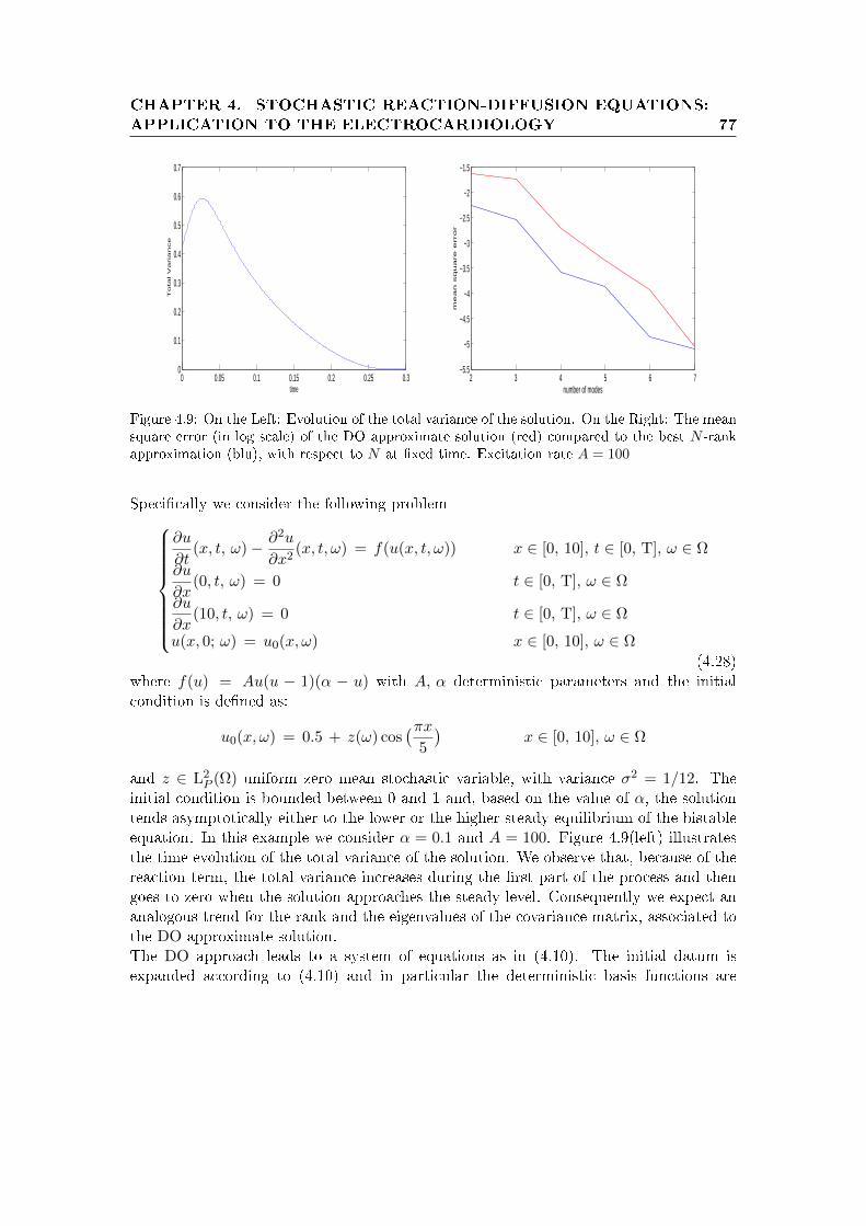
CHAPTER 4. STOCHASTIC REACTION-DIFFUSION EQUATIONS:
APPLICATION TO THE ELECTROCARDIOLOGY 77
0 0.05 0.1 0.15 0.2 0.25 0.30
0.1
0.2
0.3
0.4
0.5
0.6
0.7
time
To
tal V
aria
nce
2 3 4 5 6 7−5.5
−5
−4.5
−4
−3.5
−3
−2.5
−2
−1.5
number of modes
me
an
sq
ua
re
erro
r
Figure 4.9: On the Left: Evolution of the total variance of the solution. On the Right: The meansquare error (in log scale) of the DO approximate solution (red) compared to the best N -rankapproximation (blu), with respect to N at xed time. Excitation rate A = 100
Specically we consider the following problem
∂u
∂t(x, t, ω)− ∂2u
∂x2(x, t, ω) = f(u(x, t, ω)) x ∈ [0, 10], t ∈ [0, T], ω ∈ Ω
∂u
∂x(0, t, ω) = 0 t ∈ [0, T], ω ∈ Ω
∂u
∂x(10, t, ω) = 0 t ∈ [0, T], ω ∈ Ω
u(x, 0; ω) = u0(x, ω) x ∈ [0, 10], ω ∈ Ω
(4.28)where f(u) = Au(u − 1)(α − u) with A, α deterministic parameters and the initialcondition is dened as:
u0(x, ω) = 0.5 + z(ω) cos(πx
5
)x ∈ [0, 10], ω ∈ Ω
and z ∈ L2P (Ω) uniform zero mean stochastic variable, with variance σ2 = 1/12. The
initial condition is bounded between 0 and 1 and, based on the value of α, the solutiontends asymptotically either to the lower or the higher steady equilibrium of the bistableequation. In this example we consider α = 0.1 and A = 100. Figure 4.9(left) illustratesthe time evolution of the total variance of the solution. We observe that, because of thereaction term, the total variance increases during the rst part of the process and thengoes to zero when the solution approaches the steady level. Consequently we expect ananalogous trend for the rank and the eigenvalues of the covariance matrix, associated tothe DO approximate solution.The DO approach leads to a system of equations as in (4.10). The initial datum isexpanded according to (4.10) and in particular the deterministic basis functions are

CHAPTER 4. STOCHASTIC REACTION-DIFFUSION EQUATIONS:
APPLICATION TO THE ELECTROCARDIOLOGY 78
initialized as:
ui(x, 0) =
√1
5cos
((i− 1)πx
5
)i = 1, ..., N
that implies:
u0(x, t) = u(x, 0) +
N∑i=1
yi(0, ω)ui(x, 0) x ∈ [0, 10], ω ∈ Ω
where u(x, 0) = 0.5, y2(0, ω) =√
5z(ω) and yi(0, ω) = 0 for all i = 1 and i = 3, ..., N .It follows that the rank of the covariance matrix is initially equal to one. Figure 4.10(left) conrms the expected evolution of the rank of the covariance matrix. Contrary towhat discussed in the Chapter 3, even if the initial condition is a 1-rank function, thesolution evolves in a multidimensional manifold. This is due to the presence of the nonlinear reaction term and it means that more terms in the DO expansion are needed towell describe the solution. On the other hand gure 4.10 (right) shows that, even if manystochastic coecients are activated during the process, only few of them reach relevantlevels of variance. This means that good level of approximation can be still achievedby using few modes. More precisely we consider the error in norm L2(D) ⊗ L2
P (Ω)at time t xed. In the Figure 4.9 (right) we compare the error of the DO approximatesolution with that of the best N -rank approximation with respect to N . The best N rankapproximation, that corresponds to the truncated KL expansion is computed numericallyby using the solution computed through the Stochastic Collocation method with Ny = 41collocation points. The gure shows that by increasing N , the error of the DO methoddecreases more or less at the same rate as the best approximation error. Moreover goodlevel of accuracy can be achieved with few modes.
4.5.1 Comparison with the Stochastic Collocation method
The Stochastic Collocation method and the DO approach are based on two dierentconcepts of approximation. Given a stochastic eld u ∈ L∞([0, T], L2(D)⊗L2
P (Ω)) thatis a solution of a problem as in (1.28), the Stochastic Collocation method provides, at anytime step, a global polynomial approximation of u in the stochastic space, interpolatory inthe case of tensor grids or nested collocation points, that is built upon specic evaluationsof the time dependent process in the collocation points. On the contrary the DO methoddevelops an approximate solution that is a linear combination of few basis functionswhich depend on the solution and which aim to globally approximate it. However, theDO method described in this thesis is closely related to the Stochastic Collocation methodsince the latter is used to solve the ODEs for the stochastic coecients in (2.6). It followsthat the error of the DO solution, in mean square sense, is related to the error of theStochastic Collocation method. Specically, by using the same number of collocationpoints, the error of the Stochastic Collocation method represents a lower bound for theDO method. Indeed, according to the numerical methods used to solve the DO system,

CHAPTER 4. STOCHASTIC REACTION-DIFFUSION EQUATIONS:
APPLICATION TO THE ELECTROCARDIOLOGY 79
0 0.05 0.01 0.15 0.2 0.25 0.3 0.35 0.40
5
10
15
20
25
30
time
ra
nk
0.05 0.1 0.15 0.2 0.25 0.3 0.35 0.4−16
−14
−12
−10
−8
−6
−4
−2
0
time
eig
en
va
lue
s
Figure 4.10: On the left: The rank evolution with N = 10, 20, 30 and corresponding number ofcollocation points Ny = N + 1. Excitation rate A = 100. On the right: Time evolution of theeigenvalues, in logarithmic scale with N = 30. Excitation rate A = 100.
the approximate solution can be expanded as:
uN (x, t; ω) = u(x, t) +∑N
i=1 yi(t; ω)ui(x, t)
= u(x, t) +∑Ny
j=1
[∑Ni=1 yi(t; ξj(ω))ui(x, t)
]Lj(ξ(ω))
(4.29)
that coincides to the approximate solution of the Stochastic Collocation method if N =Ny − 1. It follows that the error of the DO method is bigger than the error of theStochastic Collocation method when we use the same number of collocation points andN < Ny − 1. On the other hand it is interesting to verify how much the error increasesby decreasing N . In gure 4.11 (left) we compare the DO solution computed with Ny
collocation points to the solution obtained through the Stochastic Collocation methodwith the same Ny, by varying the number of modes N . Specically the plot concerns thenumerical test discussed in the section 4.28 and the error computed is dened as:
ε(N) =1
T
∫ T
0‖uN (·, t, ·)− usc(·, t, ·)‖L2(D)⊗L2
P (Ω)dt
where usc denotes the solution of Stochastic Collocation method with Ny = 21. In thegure 4.11 (right) we instead compare two solutions obtained by the DO method withdierent number of collocation points. We computed the error of the two approximatesolutions with dierent values of N . We considered the error in mean square sense, withrespect to a reference solution computed through the Stochastic Collocation method withmany more collocation points. The plot shows that in the case analyzed, for small valuesof N , the trend of the error is independent to the the number of collocation points.Moreover it conrms that is not reasonable to use N > Ny.

CHAPTER 4. STOCHASTIC REACTION-DIFFUSION EQUATIONS:
APPLICATION TO THE ELECTROCARDIOLOGY 80
2 4 6 8 10 12 14 16 18 20−16
−14
−12
−10
−8
−6
−4
−2
number of modes
ε
2 4 6 8 10 12 14 16 18 20−16
−14
−12
−10
−8
−6
−4
−2
number of modes
me
an
sq
ua
re
erro
r
Figure 4.11: On the left: the error of the DO method compared to the Stochastic Collocationmethod, with the same number of collocation points Ny = 21, with respect to N (log scale). Onthe right: The error of the DO solution with Ny = 11 (green) and Ny = 21(blu) compared to areference solution, with respect to N
4.6 Adaptive Dimensionality
In this section we describe an adaptive method for the dimensionality of the mani-fold where the solution is approximated, by following the criteria introduced in [17] [16].According to the DO approach described in the Chapter 2, given N , the approximate so-lution is represented in terms of N deterministic orthonormal basis functions associatedto N stochastic coecients. Adaptive methods basically consist in supposing N a func-tion of time. A number of modes that is xed in time and chosen a priori leads indeedto two important questions: how many basis functions are needed to well describe thesolution during the whole time interval and how is it possible to minimize this number?The DO approach gives a rst answer to the problem by looking directly for a low rankapproximate solution with a spectral representation as in (2.1). On the other hand thereare many situation in which the low rank approach is not a suitable choice. The bistableequation with stochastic threshold potential value described in the section (4.4) providesan example. In that case indeed the eective rank of the solution, that is initially equalto zero for deterministic initial conditions, grows fast up to high levels and then decreasesagain to zero. Adaptive dimensionality criteria aim to use a time dependent number ofmodes N(t) that follows the trend of the eective rank of the solution in order to obtainat any time instant an approximate representation which uses only the minimum numberof terms to achieve the accuracy required. The focal points of these approaches concernsthe choice of the basis functions to add or drop out.

CHAPTER 4. STOCHASTIC REACTION-DIFFUSION EQUATIONS:
APPLICATION TO THE ELECTROCARDIOLOGY 81
4.6.1 Decreasing the dimensionality
The criterion to reduce the dimensionality is based on the rank of the covariancematrix. If the covariance matrix is singular, the basis functions associated to the zerovariance stochastic coecients, are dropped. In oder to do this we use the observation in(2.21). First of all we underline that, according to adaptive criteria, the dimension of thecovariance matrix changes in time, i.e. C(t) ∈ RN(t)×N(t). Being λ1(t), ..., λN(t)(t) andv1(t), ...vN(t)(t) the sequences of the eigenvalues and eigenvector of the covariance matrixat time t, the approximate solution uN ∈ MN can be expressed in terms of orthogonalcomponents in both the physical and stochastic space:
uN (x, t; ω) = u(x, t) +
N(t)∑i=1
zi(t; ω)wi(x, t) (4.30)
where
• wj(x, t) =∑N(t)
i=1 ui(x, t)vi j(t)
• zj(t; ω) =∑N(t)
i=1 yi(t; ω)vj i(t)
Moreover one can verify that the basis functions w1, ..., wN(t) correspond to the principalcomponents of the approximate solution. Let w and z be the vector of functions suchthat w(x, t) =
(w1(x, t), ..., wN(t)(x, t)
)and z(ω, t) =
(z1(ω, t), ..., zN(t)(ω, t)
)and D the
diagonal matrix of the eigenvalues, it holds:
Cu(t)u(t)(x, x′) = E[w(x, t)z>(t, ·)z(t, ·)w>(x′, t)] = w(x, t)D(t)w>(x′, t) (4.31)
Reminding that the basis functions are orthonormal in L2(D), it is easy to check thatλ1(t), ..., λN(t)(t) and w1, ..., wN(t) are the solutions of the eigenvalue problem associatedto Cu(t)u(t). In light of that, if the covariance matrix singular with one zero eigenvalue,we drop the basis function associated to the zero eigenvalue and the dimensionality isreduced to N(t+) = N(t) − 1. In practice, from a computational point of view, we xa threshold under which the stochastic coecients are considered having zero variancestochastic variables and at any time step we check if any random coecient is under thethreshold, in which case it is dropped.
4.6.2 Increasing the dimensionality
Given a stochastic problem as in (1.28), the DO method develops an approximatesolution in the manifolds MN that is mapped by the N orthonormal basis functionsu1, ..., uN at any time instant. Following the adaptive dimensionality approach, we denotewithWN(t) the N(t) dimensional subspace spanned by u1, ..., uN(t) and, at the xed timeinstant t∗ ∈ [0, T], we look for the direction in the subspace orthogonal toWN(t∗), thatis associated the largest potential variance. Let us rst explain the idea by applyingthe it to the truncated KL expansion, to which the DO approach is inspired. Fixed thetime instant t∗ and the number of basis functions N∗ = N(t∗), the method aims to add

CHAPTER 4. STOCHASTIC REACTION-DIFFUSION EQUATIONS:
APPLICATION TO THE ELECTROCARDIOLOGY 82
the (N∗ + 1)th principal component of u if the associated eigenvalue is bigger than thethreshold. By transferring this idea in the DO framework, we underline that the basisfunction to add is a priori unknown. We followed the approach proposed in [16], [16]according to which we study the stability of the reduced system to perturbation normal toWN(t) by computing the Normal Innitesimal Lyapunov Exponents introduced in [35] tostudy the normal stability proprieties of invariant manifolds. In view of that we dene theFréchet derivative that is a basic element for optimization problems involving functionalderivatives. Let X and Y be two Banach spaces and F : A ⊂ X → Y with A open inX. F is Fréchet dierentiable in x ∈ U if there exists a linear operator dF (x) : X → Ysuch that for any x+ h ∈ U it holds:
limh→0
‖F (x+ h)− F (x)− dF (x)h‖Y‖h‖X
= 0 (4.32)
Let uN∗ ∈ MN∗ the approximate solution at t = t∗ , we seek a new basis function u∗ ∈W>N∗ orthonormal in L2(D) to u1, ..., uN∗. Let uN∗+1 be the perturbed approximatesolution dened as:
uN∗+1(x, t∗, ω) = uN∗(x, t∗, ω) + hy∗(t∗, ω)u∗(x, t∗) x ∈ D, ω ∈ Ω (4.33)
where 0 < h << 1. We assume y∗(t∗, ·) ∈ L2P (Ω) is a random variable with zero mean
and independent to y1(t∗, ω), ..., yN∗(t∗, ω) . By deriving the DO equations as in (2.6)
we obtain:
h∂y∗(t, ω)
∂t=< L(uN∗+1(·, t, ω); ω) − E[L(uN∗+1(·, t, ω); ω)], u∗(·, t∗) > (4.34)
Supposed L Fréchet dierentiable in L2(D), it holds:
L(uN∗+1(x, t, ω), ω) = L(uN∗(x, t, ω), ω) +hy∗(t, ω)dL(uN∗(x, t, ω), ω)u∗(x, t) + o(h2)(4.35)
Being y∗ a zero mean stochastic process, the expected value of (4.35) at t→ t∗ leads to:
limt→t∗
E[L(uN∗+1(x, t, ·))] = limt→t∗E[L(uN (x, t, ·))] + o(h2) (4.36)
By replacing (4.36) and (4.35) in (4.34) for t→ t∗ we get:
limt→t∗ h∂y∗(t, ω)
∂t=< L(uN (·, t∗, ω); ω) − E[L(uN (·, t∗, ω); ω)], u∗(·, t∗) > +
hy∗(t∗, ω) < dL(uN (·, t∗, ω), ω)u∗(x, t), u∗(x, t∗) > + o(h2)(4.37)
Then we multiply by y∗ and integrate in Ω. By using again that y∗ is a zero meanstochastic process and that it is independent of y1, ..., yN∗ when h that tends to zero ityields:
dE[(y∗(t∗, ·))2]
dt= 2E[y∗(t∗, ·)2] < E[dL(uN (·, t∗, ω), ω)u∗(·, t∗)], u∗(·, t∗) > (4.38)

CHAPTER 4. STOCHASTIC REACTION-DIFFUSION EQUATIONS:
APPLICATION TO THE ELECTROCARDIOLOGY 83
Finally the basis function that we are looking for is given by the u∗ ∈ W>N∗ orthonormalin L2(D) that maximizes:
Q(v) =< E[dL(uN (·, t∗, ω), ω)v∗(·, t∗)], v(·, t∗) > (4.39)
under the assumption that all the stochastic variables associated to the basis functionsnot included in WN∗ have the same variance.
4.6.3 An heuristic approach
In this section we give an heuristic criterion to increment the dimensionality. It isbased on verifying if there is any direction, along which the solutions evolves, that canpotentially develop stochasticity. The direction we look for lives in the complementaryof the stochastic subspace generated by the random variable already included in theapproximation. In light of that we can assume that the subspace spanned by the newbasis function is included in E[L(u(x, t, ·), ·)] and it is governed by the equation for themean eld in the DO system (2.6). According to the DO approach, we have:
∂baru(x, t)
∂t= E[L(u(x, t, ·), ·)]
Once discretized the time derivative of the mean function by a nite dierence, we projectit onto the orthogonal to WN :
u∗(x, tn) = ΠWN>
(u(x, tn+1)− u(x, tn)
)/∆t
We assume that y∗ is the stochastic coecient associated to u∗. At t = tn, y∗ is identicallyzero since the u∗ is not included in the stochastic space. In order to verify if y∗ is goingto increase its variance, according to the DO approach, we estimate:
∂y∗(t; ω)
∂t=< L(u(·, t; ω); ω) − E[L(u(·, t; ω); ω)], u∗ >
At the discretized level, since y∗ is identically zero at tn we have:
y∗(tn+1; ω) =< L(u(·, tn+1; ω); ω) − E[L(u(·, tn+1; ω); ω)], u∗ > ∆t
Then by computing [E[y∗(tn+1, ·)2] we have an estimate of the variance along the directionu∗. If that variance is bigger than a threshold we orthonormalize u∗ and we include it inthe stochastic subspace.
4.6.4 Numerical approach
We give here a brief idea of a possible numerical approach for problem (4.39) We haveseen in Section 4.6.1 that the problem of adding the new mode can be re-interpreted inthe optimization problem in (4.39). From the computational point of view we adoptthe strategy proposed in [16], [17] which consists in sampling the space orthogonal to

CHAPTER 4. STOCHASTIC REACTION-DIFFUSION EQUATIONS:
APPLICATION TO THE ELECTROCARDIOLOGY 84
0 0.5 1 1.5 2 2.5 3 3.5 4 4.5 50
5
10
15
20
25
30
35
40
time
rank
DO N=40DO
he
DOad
Figure 4.12: The evolution of the rank of the DO approximate solution (blu) with N = 40, ofthe adaptive DO solution (red) with approach in 4.6.4, adaptive DO solution with the heuristicapproach (green) in 4.6.3
WN (that is the subspace spanned by the basis functions already in the expansion 2.1of the DO approximate solution). With this aim we apply the Gram-Schmidt methodto a nite set of N2 Fourier basis functions. Alternative we select a nite set of Fourierbasis functions and them we project them into the orthogonal to WN . Say φ1, ..., φN2
the sampling basis functions, then mode which we are looking for is written as:
u∗(x, tn) =
N2∑i=1
a∗iφi(x) (4.40)
and 4.39 is reduced to:
Q(v)n = aiaj < E[dL(uN (·, tn, ω); ω)φi], φj >
with v =∑N2
i=1 aiφi(x) Dened
Qij =< E[dL(uN (·, tn, ω); ω)φi], φj >
the problem 4.39 is reduced to the optimization of the quadratic functional Q =1
2(Qij +
Qji) and in conclusion the new basis function is choice to correspond to the eigenvectorassociated to the maximum eigenvalues of Q.
4.6.5 Illustrative example
We apply the method proposed in [16] as well we tested the heuristic approach in 4.6.3to problem (4.24). This represents a challenging example since the rank of the covariance

CHAPTER 4. STOCHASTIC REACTION-DIFFUSION EQUATIONS:
APPLICATION TO THE ELECTROCARDIOLOGY 85
matrix fast increases up to large values. Figure 4.12 shows the evolution of the rank ofthe DO approximate solution with N = 40 and the rank of the adaptive approximatesolutions. Observe that for the adaptive solution the rank corresponds to the number ofmodes. Figure 4.12 shows that the dimension of the adaptive solutions well follows thetrend of the rank of the DO approximate solution, which arrives up to the saturationlevel. We remark that this section concerns starting results about the adaptive approachfor the DO method, but however they are encouraging for further analysis.

Chapter 5
Conclusion
In this thesis we have investigated a low rank approximation method concerning theDynamically Orthogonal approach for time dependent PDEs with stochastic parametersor initial data. This consists in developing an approximate solution expanded in termsof mean eld, stochastic coecients and deterministic basis functions, all of them timedependent that adapt to the solution as it evolves. Without imposing any polynomialstructure to the term of the expansion we directly look for an approximate solution ofthe form in DO. This is achieved by projecting at any time instant the residual of thegoverning SPDE in (2.5) onto the tangent space to MN , MN the manifold where allthe rank N stochastic elds. Then we recover a coupled system of evolution equationsfor all the terms of the expansion (2.1), which consists in N+1 deterministic PDEs plusN stochastic ODEs. This allows to evolve a low rank solution that adapts at each timeinstant both the basis functions and the deterministic coecients to what best describesthe global structure of the solution. This idea suggests some relationships between theDO approximate solution and the N-truncated KL expansion.On the other hand we showed that the DO approach and DDO decomposition providethe same numerical solution if a Galerkin formulation is adopted. This is a remarkableand encouraging starting point since convergence and error estimates are present in theliterature for the DDO decomposition in nite dimensional setting. In particular it isshown that for evolution matrix equations the error of the DDO approximate solutionis bounded in terms of optimal approximation error, under specic conditions. In lightof that we investigated the relationships between the DO approach and the N truncatedKL expansion, that is a representation of the best N rank approximation in mean squaresense. We rst focused on liniar parabolic diusion equations with initial stochasticcondition. In this framework theoretical considerations, conrmed by numerical tests,show that the DO approximate solution coincides with the optimal one only under verystrong assumptions and that generally the convergence rate of the error is determinedby the smallest eigenvalue of the Laplace operator. However we remark that the KLexpansion does not represents an alternative method to the DO approach but a lowerbound for the approximation error. Encouraging numerical results are provided by theanalysis of the more challenging problem, governed by a parabolic diusion equations with

CHAPTER 5. CONCLUSION 87
non linear reaction term with initial stochastic condition, where we see that the error ofDO approximate solution results is proportional to the optimal error and decreases withthe same rate. In conclusion, even if the question remains already open, the achievedresults make the DO approach suitable to a further analysis. In view of that, the probablymore interesting feature of the DO approach concerns the adaptability of the dimension.As we have seen in the analysis of parabolic equations with non linear reaction term,during the evolution of the process the eective rank of the solution might signicantlychange. If decreasing the dimensionality is an easy task, the questions concerning whenadd and how to select new directions is already open. The starting results show that thisis suitable and eective approach and furthermore several strategies can be investigated.We tested the idea of dimension adaptability by following the approach proposed in [17],[16] which consists in sampling the space orthogonal to the modes already included inthe approximation, but more eective method can be investigated. One of the morepromising is maybe a method based on power-type or Arnoldi iteration, in the samespirit as what proposed in [37].

Bibliography
[1] I. T. Jolli e, Principal component analysis, second ed., Springer Series in Statistics(SpringerVerlag, 2002).
[2] O.P. Le Maitre, O.M. Knio, Spectral methods for uncertainty quantifcation, Springer,2010.
[3] F. Nobile and R. Tempone. Analysis and implementation issues for the numericalapproximation of parabolic equations with random coecients. Int. J. Num. Meth-ods Engrg., 80(6-7): 979-1006, 2009. Special Issue: Uncertainty Quanti cation inComputational and Prediction Science.
[4] I. Babuska, R. Tempone, and G. E. Zouraris, Galerkin nite element approximationsof stochastic elliptic partial dierential equations, SIAM J. Numer. Anal. 42 (2004)800-825.
[5] S. Salsa, Partial Dierential Equations in Action: From Modelling to Theory,Springer-Verlag, 2008
[6] R.J. Alder, J.E. Taylor, Random Fields and Geometry, Springer, 2007
[7] F. Nobile, R. Tempone, C. G. Webster, A sparse grid stochastic collocation methodfor partial dierential equations with random input data. SIAM Journal, Vol. 46,No.5, pp. 2309-2345
[8] X. Wan and G.E. Karniadakis. Long-term behavior of polynomial chaos in stochas-tic ow simulations. Comput. Methods Appl. Mech. Engrg., 195(41-43): 5582-5596,2006. Art 5 da citare
[9] H. G. Matthies and A. Keese. Galerkin methods for linear and nonlinear ellip-tic stochastic partial dierential equations. Comput. Methods Appl. Mech. Engrg.,194(12-16):1295 1331, 2005.
[10] C. Lubich, T. Rohwedder, R. Schneider, and B. Vandereycken. Dynamical approxi-mation of hierarchical tucker and tensor-train tensors. MATHICSE Technical Report28.2012, École Polytechnique Fédérale de Lausanne, 2012.
[11] O. Koch and C. Lubich. Dynamical tensor approximation. SIAM J. Matrix Anal.Appl., 31(5):2360 2375, 2010.

BIBLIOGRAPHY 89
[12] O. Koch and C. Lubich. Dynamical low-rank approximation. SIAM J. Matrix Anal.Appl., 29(2):434 454, 2007.
[13] V. Heuveline and M. Schick. A local time dependent generalized polynomial chaosmethod for stochastic dynamical systems. EMCL Preprint Series 04, EMCL, Karl-sruhe Institute of Technology, 2011.
[14] M. Gerritsma, J-B. van der Steen, P. Vos, and G. Karniadakis. Time-dependentgeneralized polynomial chaos. J. Comput. Phys., 229(22):8333-8363, 2010.
[15] M.S. Eldred. Recent advances in non-intrusive polynomial chaos and stochastic col-location methods for uncertainty analysis and design. In AIAA, 2009.
[16] Themistoklis P. Sapsis, and Pierre F.J. Lermusiaux, Dynamical criteria for the evolu-tion of the stochastic dimensionality in ows with uncertainty, Physica D, 241(2-12)60-76.
[17] Themistoklis P. Sapsis and Pierre F.J. Lermusiaux, Dynamically orthogonal eldequations for continuous stochastic dynamical systems, Physica D, 238 (2009) 2347-2360.
[18] F. Nobile, R. Tempone and C. Webster, An anisotropic sparse grid stochastic col-location method for partial dierential equations with random input data, SIAM J.Numer. Anal., 2008, vol. 46/5, pp. 2411-2442.
[19] M. P. Ueckermanna, P. F. J. Lermusiauxa, and T. P. Sapsis, Numerical Schemesfor Dynamically Orthogonal Equations of Stochastic Fluid and Ocean Flows, J.Comput. Phys., submitted
[20] A. Quarteroni A. Valli Numerical Approximation of Partial Dierential Equations.Springer-Verlag, Berlin Heidelberg, 1994
[21] J. Beck, F. Nobile, L. Tamellini, R. Tempone, Optimal polynomial approximation ofstochastic PDEs by Galerkin and Collocation methods MOX report, 23/2011.
[22] I. Babuska, F. Nobile, R. Tempone, A stochastic collocation method for ellipticpartial dierential equations with random input data, SIAM REVIEW Vol. 52, No.2, pp. 317-355.
[23] R. G. Ghanem and P. D. Spanos, Stochastic nite elements: a spectral approach(Springer Verlag, 1991).
[24] B. Ganapathysubramanian and N. Zabaras, Sparse grid collocation schemes forstochastic natural convection problems, Journal of Computational Physics 225(2007) 652-685.
[25] N. Wiener, The homogeneous chaos, American Journal of Mathematics 60 (4) (1938)897-936.
BIBLIOGRAPHY 90
[26] D. Xiu, G. Karniadakis, The Wiener-Askey polynomial chaos for stochastic dier-ential equations, SIAM Journal on Scientic Computing 24 (2) (2002) 619-644.
[27] J. Stoer, R. Bulirsch, Introduction to Numerical Analysis, Springer-Verlag, NewYork, 1979.
[28] A.J. Pullan, M.L. Buist, L.K. ChengMathematically Modelling the Electrical Activityof the Heart World Scientic Co. Pte. Ltd.
[29] J. Keener, J. Sneyd Mathematical Physiology Springer
[30] R.H. Cameron, W.T. Martin, The orthogonal development of non-linear functionalsin series of Fourier-Hermite functionals, Annals of Mathematics 48(2) (1947) 385-392.
[31] R. A. Todor and C. Schwab. Convergence rates for sparse chaos approximationsof elliptic problems with stochastic coe cients. IMA J Numer Anal, 27(2):232-261,2007.
[32] A. Cohen, R. Devore, and C. Schwab. Analytic regularity and polynomial approxi-mation of parametric and stochastic elliptic PDE's. Anal. Appl. (Singap.), 9(1):11-47, 2011.
[33] D. Xiu and J.S. Hesthaven. High-order collocation methods for dierential equationswith random inputs. SIAM J. Sci. Comput., 27(3):1118-1139,2005
[34] T. Zhou, F. NobileOn Dynamically Orthogonal Fields Approach for Time Depen dent Stochastic PDEs,in preparation
[35] G. Haller and T.P. Sapsis. Localized instability and attraction along invariant man-ifolds. SIAM J. of Appl. Dynamical Systems, 9:611-633, 2010
[36] G.wanner, E.Hairer, C. Lubich Geometric Numerical Integrtion: Structure-Preserving Algorithms for Ordinary Dierential Equations, Springer
[37] L. Tamellini, O. Le Maitre, and A. Nouy. Model reduction based on proper general-ized decomposition for the stochastic steady incompressible navier-stokes equations.MOX-Report 26/2012, Department of Mathematics, Politecnico di Milano, Italy,2012. submitted