Copyright Warning & Restrictions

The copyright law of the United States (Title 17, United States Code) governs the making of photocopies or other

reproductions of copyrighted material.

Under certain conditions specified in the law, libraries and archives are authorized to furnish a photocopy or other

reproduction. One of these specified conditions is that the photocopy or reproduction is not to be “used for any

purpose other than private study, scholarship, or research.” If a, user makes a request for, or later uses, a photocopy or reproduction for purposes in excess of “fair use” that user

may be liable for copyright infringement,

This institution reserves the right to refuse to accept a copying order if, in its judgment, fulfillment of the order

would involve violation of copyright law.

Please Note: The author retains the copyright while the New Jersey Institute of Technology reserves the right to

distribute this thesis or dissertation

Printing note: If you do not wish to print this page, then select “Pages from: first page # to: last page #” on the print dialog screen

The Van Houten library has removed some of the personal information and all signatures from the approval page and biographical sketches of theses and dissertations in order to protect the identity of NJIT graduates and faculty.

ABSTRACT

Title of Thesis: Statistical Multiplexing of Video Sources

For Packet Switching Networks

Krishna Kancherla, Master of Science in Electrical Engineering, 1989

Thesis Directed by: Dr. Constantine Manikopoulos, Associate Professor

Communication networks are fast evolving towards truly integrated networks han-

dling all types of traffic. They employ integrated switching technologies for voice,

video and data. Statistical or asynchronous time division multiplexing of full mo-

tion video sources is an initial step towards packetized video networks. The main

goal is to utilize the common communication channel efficiently, without loosing

quality at the receiver. This work discusses the concept of using statistical multi-

plexing for packet video communications. The topology of a single internal packet

network to support ISDN services has been adoptedf Simulations have been car-

ried out to demonstrate the statistical smoothing effect of packetized video in

the networks having high speed links. Results indicate that the channel rate per

source decreased in an exponential manner as the number of sources increased.

An expression for the average usage time t of the channel has been derived in

terms of channel rate per source and the number of sources multiplexed. Also

the average usage time of the channel is higher for buffered data than that of the

multiplexed data. The high speed communication links in the internal network

are lightly loaded, which indicates that these links can accommodate more data.

STATISTICAL MULTIPLEXINGOF VIDEO SOURCES

FOR PACKET SWITCHINGNETWORKS

byKrishna Kancherla

Thesis submitted to the Faculty of Graduate School of.the New Jersey Institute of Technology in partial fulfillment of

the requirements for the degree ofMaster of Science in Electrical Engineering

1989

APPROVAL SHEET

Title of Thesis: Statistical Multiplexing of Video SourcesFor Packet Switching Networks

Name of Candidate: Krishna KancherlaMaster of Science in Electrical Engineering, 1989

Thesis & Abstract Approvedby the Examining Committee:

Dr. Constantine N. Manikopoulos, Advisor DateAssociate ProfessorDepartment of Electrical and Computer Engineerig

Nirwan Ansari DateAssistant ProfessorDepartment of Electrical and Computer Engineering

Dr. Irving Wag DateAssistant ProfessorDepartment of Electrical and Computer Engineering

New Jersey Institute of Technology, Newark, New Jersey.

VITA

Name: Krishna Kancherla

Present address:

Degree and date to be conferred: M.S.E.E., 1989

Date of birth:

Place of birth:

Secondary Education: K.T.R. Women's College, India, 1981

Collegiate institutions attended Dates Degree Date of Degree

Andhra University 1981-85 B.S.E.E 1985

New Jersey Institute of Technology 1987-89 M.S.E.E 1989

Major: Electrical Engineering

Positions held: Graduate Assistant, Honors Program, NJIT

Acknowledgement

I wish to express my sincere thanks to Dr. Constantine N. Manikopoulos for his

valuable guidance and encouragement throughout the course of this thesis. I am

specially indebted to him for his insightful and constructive criticisms at every

stage of this thesis without which this thesis would never have been completed. I

also express my thanks to Dr. Irving Wang and Dr. Nirwan Ansari who served

on this thesis committee and made appropriate suggestions. I also express my

sincere thanks to Mr. Jagadish Rangwani for his helpful discussions of Network

11.5 simulation package at every stage of this work. Last but not the least I would

like to thank all those who have helped me in one way or the other during the

entire course of this thesis.

Chapter 1

1. Introduction 1

Chapter 2

2. Packet Switching Networks

2.1 Introduction 4

2.2 Attractive Features of Packet Switching 5

2.3 Statistical Multiplexing

2.3.1 Introduction 7

2.3.2 Statistical Multiplexing compared with TDM and FDM f.. 12

2.3.3 Using one Vs. Multiple Channels 13

2.4 Network Architecture 14

2.5 Conclusions 19

Chapter 3

3. Packet Video Communications

3.1 Introduction 20

3.2 Modeling and Analysis Assumptions 23

3.3 Source Models

3.3.1 Model A: Continuous-State, Discrete-Time Markov Model . 28

3.3.2 Queueing Simulation Using Model A 29

3.3.3 Model B: Discrete-State, Continuous-Time Markov Process 30

3.3.4 Queueing Analysis Using Model B 37

3.4 Conclusions 40

Chapter 4

4. Simulation Model

4.1 System Characteristics 41

4.2 Simulation Results 44

4.3 Conclusions 58

Chapter 5

5.Conclusions 59

Appendix 1 61

Bibliography 66

List of Figures

Fig 2.1 Statistical Multiplexing 9

Fig 2.2 Transmission Speed Vs. Delay 11

Fig 2.3 Basic Process of Packet Data 15

Fig 2.4 Network Architecture 17

Fig 3.1 Statistical Multiplexer of N Sources 24

Fig 3.2 Bit rate histogram 27

Fig 3.3 Poisson Sampling & Quantization of Source rate 31

Fig 3.4 State Transition Diagram - Model B 33

Fig 3.5 Minisource Model 36

Fig 4.1 Simulation Model 42

Fig 4.2 % Utilization of High Speed Chanel 45

Fig 4.3a Chanel rate/source Vs. No. of Sources 46

Fig 4.3b Logλ(n) Vs. No. of Sources 47

Fig 4.3c Chanel rate/source derived from eq.(4.7) 48

Fig 4.4a Average Usage Time of High Speed Chanel Vs. No. of Sources 50

Fig 4.4b Logλ(n)e-t Vs. No. of Sources 51

Fig 4.5a Chanel rate/source Vs. No. of Sources 2Mbit buffer 53

Fig 4.5b Chanel rate/source Vs. No. of Sources 3.9Mbit buffer 54

Fig 4.6 Average Usage Time of Channel with & without buffer 55

List of Tables

Table 4.1 % Utilizations of links in the Network 56

Table 4.2 % Utilizations of Packet Switches in the Network 57

Chapter 1

Introduction

The increasing popularity of packet switching to handle data, voice and video

integrated services has resulted in great concern for high network congestion lev-

els and packet losses due to buffer delays. As video is expected to be a major

traffic component on Integrated Services Digital Networks (ISDN's), it is very

important to transmit image of constant quality with variable transmission rate.

High capacities have been made possible by the increasing use of optical fiber

links and the development of highly sophisticated VLSI communication devices.

But as more bandwidth becomes available due to the use of optical fiber links,

more services are designed to use them up. Besides loading the communication

lines, switched broad-band services impose large loads on the switches; this is of

great concern, if the switching in networks of future will use an integrated flexible

technology such as fast packet switching for voice, video and data alike. The high

traffic congestion is expected in the context of a network serving a large number

1

of identical, independent, statistical sources.

This work discusses the concept of using statistical multiplexing for packet

switching networks to support ISDN services, particularly for video sources. Sim-

ulation studies has been done to study the network performance under increasing

load conditions. Also the transmission efficiency of the high speed links has been

studied as the number of sources increases.

Packet switching of variable bit-rate real-time video sources is a means for

the efficient sharing of communication sources, while maintaining uniform picture

quality. Variable bit-rate video coding exhibits the type of statistical variations

that made packet switching attractive for bursty traffic. Advantages of packet

switching over conventional circuit switching, and the transmission efficiency of

packet switching due to statistical multiplexing for video communication are ex-

plained in detail in chapter II. Also a network architecture that support integrated

services using high speed transmission links and high performance packet switches

has been described.

Chapter III explains two performance models of statistical multiplexing in

packet video communications. The coding bit rate of a single video source as

a function of time based on experimental data [1] of a video telephone. Two

correlated Markov process models (one in discrete time and one in continuous

time are explained to fit the experimental data that are used to model the input

rates of several independent video sources into a statistical multiplexer.

The model of variable bit rate sources derived from chapter III are used for

2

our simulation purposes. The simulation model,the bit rate data and the network

under consideration are explained in detail in chapter IV, and finally the results are

presented. Our results show that as the number of sources increase from 1 to 100

at the statistical multiplexer, the channel rate per source decreased exponentially

from 7.5 Mbits per second to 1.9 Mbits per second, while maintaining the channel

utilization at 85%. An approximate expression for the average usage time t has

been derived in terms of channel rate per source λ(n), and the number of sources

multiplexed n. Also it has been noticed that the average usage time decreased as

the number of sources multiplexed increased.

For the same data rate we have to use a buffer of size 2Mbits to get the

equivalent effect to statistical multiplexing. The buffering effect has been found

to be negligible as the number of sources increase beyond 50. The average usage

time of the channel is higher for the buffered data than that of the multiplexed

data. The links and the packet switches of the internal packet network are lightly

loaded even for large number of sources, indicating that the performance is good.

3

Chapter 2

Packet Switching Networks

2.1 Introduction

Packet switching technology has achieved a great success since it was intro-

duced in the 1970's mainly for bursty computer communications. Packet switching

is a technique widely used today in specialized data communication networks with

a growing number of actual networks working in the world today. Packet switch-

ing networks aim at offering data transmission services for multiple applications

.The integration of different types of information over such media becomes attrac-

tive for large scale economy and for better utilization of these powerful resources.

The popularity of packet switching integrated services for an increasing number

of applications is cause for concern in terms of offering good performance. Traffic

congestion has been a real problem in achieving good network performance.

Data from all users are statistically multiplexed on a shared network resources;

the moment-to-moment bandwidth requirements of individual users often vary

dramatically. Today's networks are designed for the applications of modest traffic

4

level fluctuations. But whenever it exceeds the limit, the network traffic congestion

level rises resulting in long transmission. delays, causing heavy data losses and even

sometimes blocking up the network altogether.

In the mean time, more and more new services are being introduced into packet

switching networks, such as packet voice, image data transmission and telecon-

ferencing, etc. These services demand the network to provide truly guaranteed

type-of-service ( TOS) transmissions that should meet diverse and stringent per-

formance requirements. Adequate network resources are a necessary condition for

good performance, but the resources alone do not automatically ensure a satis-

factory performance. The poor performance we see today is more due to lack of

traffic control than due to resource limitations. Theoretically, a packet switching

network can allow any single user an unlimited share of the network resources.

This is not feasible in practice due to performance criteria. Even though more

bandwidth is available due to the use of fibre optic links, these new services load

the communication lines, resulting in high congestion levels. Some aspects of

designing a new architecture for packet switching communication networks have

been discussed in [4].

2.2 Attractive Features of Packet SwitchingBesides all of the above mentioned drawbacks of packet switching technology,

there are some factors that make it an attractive method of transmission for in-

tegrated services.

5

1. Transmission Efficiency:

Many data services are characterized by bursty communications patterns which

make poor use of conventional circuit switched facilities. For example, interactive

data users typically use only a few percent of the bandwidth available to them.

Although it is less widely recognized, voice is also quite bursty. In the average

telephone conversation, less than 40% of the available bandwidth is actually used.

Packet switching can exploit this burstiness to allow many users to share the same

transmission facility.

2. Adaptability to new coding techniques:

Packet switching also makes it attractive to consider new coding techniques for

information transmission. Most information coding techniques in use today at-

tempt to maintain a smooth flow of information across the transmission facility in

order to use it efficiently. With packet switching one can exploit coding techniques

which produce bursty information streams.

3. Adaptability to changing traffic:

Packet switching naturally provides each user with exactly the bandwidth re-

quired. As new services are developed with different bandwidth requirements,

packet switching can adapt to the changing conditions much more easily than

conventional circuit switching can.

4. Integrated internal architecture:

6

Most proposals for ISDN services provide integrated access but require separate

switching networks for different types of information. Packet switching can pro-

vide both an integrated customer interface and a single network solution for a

wide range of different information transport needs, including voice, data and

video signals. Substantial cost savings could made be possible both in switching

and terminal equipment. The details of such an architecture [2] are given in sec-

tion 2.4.

2.3 Statistical Multiplexing2.3.1 Introduction:

The transmission efficiency of packet switching is due to statistical multiplex-

ing. The packets of all traffic streams are merged into a single queue and transmit-

ted on a first-come first-serve basis in sequence, one packet at a time. However,

if the queue of a traffic stream is empty, the next traffic stream is served and

no communication resource is wasted. Since the entire transmission capacity C

(bits/second) is allocated to a single packet at a time, it takes L/ C seconds to

transmit a packet that is L bits long.

In time-division (TDM) and frequency-division multiplexing (FDM) with m

traffic streams, the link capacity is essentially subdivided into m portions, one per

traffic stream. In FDM, the channel bandwidth W is subdivided into m channels

each with bandwidth W/m. The transmission capacity of each channel is roughly

C/m, where Cis the capacity that would be obtained if the entire bandwidth were

7

allocated to a single channel. The transmission time of a packet that is L bits

long is Lm/C, or m times longer than in the corresponding statistical multiplexing

scheme. In TDM, allocation is done by dividing the time axis into slots of fixed

length (e.g., one bit or one byte long, or perhaps one packet long for fixed length

packets). Again, conceptually, the communication link can be viewed as having

m separate links with capacity C/m. In the case where the slots are short relative

to packet length, the transmission time of a packet L bits long is Lm/C. In the

case where the slots are of packet length, the transmission time of an L bit packet

is L/C, but there is a wait of (m-1) packet transmission times between packets

of the same stream. One of the themes that will emerge from queueing analysis

is that the statistical multiplexing has a smaller average delay per packet than

either TDM or FDM. The main reason for the poor delay performance of TDM

and FDM is that the communication resources are wasted when allocated to a

traffic stream with a momentarily empty queue, while other traffic streams have

packets waiting in their queue.

In a conventional circuit switched network, each user is provided with a com-

munication channel that is dedicated to that user. If the user does not make use

of the available bandwidth, it is lost; there is no opportunity for making that

bandwidth available to another user. Statistical multiplexing provides a way for

customers to share transmission facilities on demand basis. This is shown in Fig-

ure 2.1. User information enters at the left, where it is broken into blocks with

a header added. This yields a packet. Packets from different sources are then

8

Fig 2.1 Statistical Multiplexing

placed in a queue and sent across the transmission facility. Upon receipt, packets

are sent to proper destinations and the original data streams are reconstructed.

Packet switching extends this idea to include the switching function, which leads

to further cost savings.

In conventional circuit switched networks, the principal source of delay is the

finite propagation speed of signals. Packet switching introduces a variable delay

due to the queueing at each outgoing transmission link. The average delay [7] can

be approximated by

where b is the packet length, n is the number of tandem links, s is the speed

of the transmission facility in bits per second, p is the average utilization of the

facility and q is the queueing delay in seconds. The delay can be decreased by

decreasing the packet length, decreasing the number of links, increasing the speed

of the transmission facility or decreasing the occupancy of the transmission facility.

Decreasing the packet length is helpful up to a point, but can lead to inefficient use

of the transmission link since as packets become shorter, a larger percentage of the

available bandwidth is used to transmit the header information rather than the

original data. Decreasing the link occupancy sacrifices the efficiency of statistical

multiplexing for speed. The number of links is a function of the size of the network

and the way that the packet switches are interconnected. The remaining variable

in the equation is the transmission speed s, which can be varied over a wide range.

10

Figure 2.2. Transmission Speed Vs. Delay

1 1

Reproducing the curve reported in [2] (fig 2, p 2.1.2), Figure 2.2 shows how the

total delay varies with transmission speed for a ten link connection spanning a

distance of 5000 miles. The minimum delay shown in the figure is due to fixed

transmission speeds that are present even in circuit switched networks.

2.3.2 Statistical multiplexing compared with TDM and FDM

Assume that m statistically identical and independent Poisson packet streams

each with an arrival rate of λ/m packets/sec are to be transmitted over a commu-

nication line [5]. The average transmission time is 1/y. If the streams are merged

into a single Poisson stream, with rate λ, like statistical multiplexing , the average

delay per packet is

If, instead the transmission capacity is divided into m equal portions, one

per packet stream as in time- and frequency-division multiplexing, each portion

behaves like an M/M/1 queue with arrival rate λ/m and average service rate

Therefore, the average delay per packet is

i.e., m times larger than for statistical multiplexing.

The preceding argument indicates that multiplexing a large number of traffic

streams on separate channels in a transmission line performs very poorly in terms

12

of delay. The performance is even poorer if the capacity of the channels is not

allocated in direct proportion to the arrival rates of the corresponding streams.

This shows that statistical multiplexing performs well when compared to TDM

and FDM.

2.3.3 Using one vs. multiple channels in statistical multiplexing

Consider a communication link serving m independent Poisson traffic streams

with rate λ/m eachf Suppose that link is divided into in separate channels with one

channel assigned to each traffic stream. However, if a traffic stream has no packet

awaiting transmission , its corresponding channel is used to transmit a packet of

another stream. The transmission times of packets on each of the channels are

exponentially distributed with mean 1/µ . The system can be modeled by the

same Markov chain as the M/M/m queue. Let us compare the average delays

per packet of this system, and an M/M/1 system with the same arrival rate λ

and service rate mil (statistical multiplexing with one channel having in times

larger capacity). In the former case, the average delay per packet is given by

where PQ is the probability that an arrival will find all servers busy and will

be forced to wait in queue and is given by

This equation is known as the Erlang C formula and is in wide use in telephony.

13

While in the case of M/M/1 system, the average delay per packet is

where PQ and PQ denote the queueing probability in each case. When p << 1

(lightly loaded system) we have

and

When p is only slightly less than 1, we have

Therefore, for a light load, statistical multiplexing with m channels produces

a delay almost m times larger than the delay of statistical multiplexing with

m channels combined in one (about the same as time- and frequency-division

multiplexing). For a heavy load, the ratio of the delays is close to one.

2.4 Network Architecture

As we discussed in section 2.1, although higher transmission speeds can reduce

queueing delay to acceptable levels, their exploitation will require a new genera-

tion of packet switching equipment. The improvements in transmission efficiency

obtainable with packet switching are dependent on the characteristics of the par-

ticular application. Packet switching is best suited to the applications that are

14

Figure 2.3 Basic Process of Packet Data

15

bursty, that is, applications that have a peak bandwidth requirement that is sub-

stantially higher than their average bandwidth requirement. Typical example is

real time video signals.

Figure 2.3 illustrates some basic processes in packetization of a signal. The

signal is first converted to digital form using an A/D converter. It is then coded

using an appropriate coding scheme depending on cost, quality and bandwidth

required. After the signal is coded, it is broken into blocks, a header is added, and

it is sent through the network. At the destination the coding process is reversed,

the signal is converted to analog and played back. Because the network introduces

a variable delay, different packets with in the same signal may experience different

delays in crossing the network. Hence, care must be taken to ensure that this effect

does not degrade the quality of the received signal.

Reviewing the motivation for constructing an integrated services network using

packet switching, a network architecture was proposed in [2]. The basic compo-

nents of this architecture are shown in Figure 2.4. They are Packet Switches (PS),

Packet Network Interfaces (PNI), High Speed Links (HSL), Customer Interfaces

(CI) and Network Administration Centers . (NA C).

There may be different kinds of PNIs depending on the nature of the access

method and services. Customers may communicate with the PNI using Digital

Subscriber Lines (DSL) having a 64 Kbs voice channel and a separate packet

mode signalling channel for voice sources. In this case the PNI would provide

voice coding and packetizing, but the far end customer would be given a voice

16

Figure 2.4. Network Architecture

17

signal as reconstructed by the far end PNI. Signalling would be handled through

messages exchanged with the CI. Another possibility is a pure Packet Line (PL)

(used in this course of work for simulation purposes). In this case the coding and

packetizing would be provided in the CI and the PNI would provide statistical

multiplexing. A third possibility is a high speed packet mode line using a protocol

similar to the internal network protocol.

The above described internal packet network architecture must have the fol-

lowing characteristics:

1. High speed digital transmission:

Modern digital transmission facilities offer higher speed and better error perfor-

mance. The simplest way to solve the delay problem is to increase the basic

transmission speed to the order of several Mbits depending on the data rate.

2. Simple internal network protocols:

The use of high speed digital transmission facilities creates opportunities for a

greatly simplified packet protocols with in the network. Simple protocols may

also be needed to ensure that fast and inexpensive protocol processors can be

built.

3. Hardware switching:

Conventional packet switches rely on general purpose computers or collection of

18

microprocessors. Novel packet switch architectures based on VLSI components

will be needed to attain high speed operation and economic implementation.

4. Separation of services from transport:

As the networks are expected to handle the frequently changing traffic, the inter-

nal network should provide basic transport without changing the parameters of

itself. The above architecture accommodates different service needs by equipment

at the access points to the internal packet network, and by special service nodes

attached to but separate from this network.

2.5 Conclusions

This chapter can be summarized as

1. Several attractive features of packet switching technology were discussed.

2. Statistical multiplexing was described in detail in comparison with TDM and

FDM.

3. The concept of using a single internal packet network to support ISDN services

was discussed.

19

Chapter 3

Packet Video Communications

3.1 Introduction

A P CM coded video signal sequence results in a large bit rate (hundreds of

Mbits/sec). In a limited bandwidth communication networks (circuit switching)

a few video sources can easily fill all line capacities. Advanced data compression

techniques are employed to transmit coded full motion video within digital lines of

lower capacity. There is a complicated tradeoff between the minimum achievable

coding rate and distortion of the decoded images. To tailor variable rate codes

into a channel of lower speed than the coding rate at very high activity, multimode

encoders equipped with buffers are used. The buffer absorbs statistical peaks of

the coding rate by temporarily storing data in excess a certain threshold, the

encoder is instructed to switch into a coding mode that has lower rate but worse

quality to avoid buffer over flow. Similarly, when buffer underflow is approached,

the channel speed is maintained by increasing the bit rate, thus improving the

quality. The efficiency of the multimode scheme increases with lower fixed speed

20

on the output line; unfortunately the quality of the received image will start

suffering from highly visible variations.

Variable bit rate video coding exhibits the type of statistical variations that

made statistical multiplexing and packet switching attractive for bursty commu-

nications. These network architectures can dynamically support variable bit rate

sources by smoothing out the aggregate of several independent streams in com-

mon buffers within the network. Hopefully, such technologies may provide effi-

cient video transmission without the unpleasant variations in quality of multimode

coders.

As explained in previous chapter, in statistical or asynchronous multiplexing,

several independent sources share a line of capacity less than the sum of their

peak rates. Instead of using individual buffers all sources feed a common buffer

and their cumulative bit rate tends to smooth out around the average rate as

indicated by the law of large numbers. We can see that packet switching is a

network extension of statistical multiplexing, with data from individual sources

segmented into small packets that are stored and forwarded from switch to switch

towards their destination. The statistical smoothing of variable rate sources is

achieved as packets are buffered in the network switches. But again, both sta-

tistical multiplexing and packet switching introduce variable delays in delivering

data due to the buffering stages. In addition, they may introduce data losses due

to buffer overflow. Thus, it is very important to select parameters and line speeds

21

to minimize these effects while maintaining the efficiency of statistical averaging.

Statistical Multiplexing of video was proposed and simulated at Bell Labora-

tories in 1972 for picturephone interframe coders [3]. Applications that require

timely and synchronous delivery, such as telephone voice and real-time video, cur-

rently use dedicated circuit switching. This may change with new concept of fast

packet switching [2], explained in previous chapter.

The asynchronous packetized transmission of conversational voice requires very

stringent end-to-end delay; voice packets exceeding a given time threshold may

not be used to synthesize the continuous voice stream at the receiver. Late packets

thus result in voice losses that can be tolerated up to a certain degree. A similar

problem is considered in full motion video in [1]. The complexity in assessing

the buffering statistics of packetized voice results from the correlated nature of

the stochastic process that models the rate of a voice source. A video source

generates correlated bit rates but of a different statistical nature. The output

of a digital voice phone alternates between talkspurts and silent periods. This

corresponds to two states for the source output rate; the state corresponding to

zero bit rate occurs 60 percent of the time. In contrast, the output rate of a

variable bit rate video coder exhibits continuous variations. Hence new models

and analytic techniques are developed in [1] to evaluate the queueing statistics

in packetized video. In this course of work we have used the data they gener-

ated using conditional replenishment interframe coding scheme for our network

simulation purposes. Hence a statistical analysis of the data and two markov

22

models that match their basic statistics are presented in the next sections. The

first model (Model A) is a continuous-state autoregressive discrete-time Markov

process which is used for simulation purposes in [1] and for ours too. The sec-

ond model (Model B) is a discrete-state, continuous-time Markov process which

is used in queueing analysis. The analytic model is used to analyze the queueing

behavior of statistical multiplexing of several independent, identically distributed

video sources. Numerical results are presented in Appendix 1.

3.2 Modeling and Analysis Assumptions

Video sources are assumed to be generating 30 frames/second. Each frame

consists of approximately 250,000 pixels that are digitally coded. Assume that

N independent video sources are multiplexed [3] into a high-speed trunk. The

unbuffered coded bits from each source are first stored in separate prebuffers and

then join a common multiplexer as in Fig. 3.1. The multiplexer assembles the

data into blocks that are transmitted over the high speed communication line. The

blocks may be asynchronous time frames that combine portions of data from each

source. The frame length depends on the instantaneous amount of data from the

sources. Frame delimiters and source identification information must be included

to enable the demultiplexing at the destination. A block may also be a packet of

data assembled from a single source. Packets are stored and forwarded in a FIFO

(first-in- first-out) mode in the same order as they are assembled. The packet

length may be variable due to temporal changes in the source bit rate, or fixed, in

23

Figure 3.1. Statiatical Multiplexer of N Sources

2 4

which case the variable source rate will cause varying packet arrival rates. Each

packet needs a header identifying the source, the destination, its sequence number,

and possibly a time stamp to alert the network in case of excessive buffering delays.

Error detection and correction overhead bits are added.

The statistical multiplexer was modeled as a queue that receives the encoded

bit streams from the prebuffers; its service rate is determined by the speed of

the high speed channel. The analysis is based on continuous fluid flow [7] ap-

proximation of the traffic that does not take into account the discrete nature of

the packets or frames. The queue behaves like a reservoir of water that is fed

from water supplies of time-varying rates and empties through a fixed-rate sink.

The analysis agrees with simulation model, in which bit streams from individual

sources are assembled into packets of fixed length.

In order to analyze the common buffer statistics, the coded source rate needs a

model. The rate depends on the compression algorithm and the nature of the video

scenef For a scene with out abrupt movement, such as the head of a talking person

in a picturephone, it is expected that the rate will have a bell-shaped stationary

probability density and to exhibit significant correlations for an interval of several

frames. This behavior has been verified experimentally in [1].

The sequence had a duration of 10 seconds or 300 frames. The instantaneous

bit rate \(t) was measured in bits/pixel. Although the measured rate is fixed for

the duration of a frame (1/30 sec), it was treated as a continuous-time function

25

since the frame period is very small compared to the time scale. Recall that there

are about 250,000 pixels per frame and 30 frames per second, thus 1 bit/pixel

corresponds to 7.5 Mbits/sec. The measured bit rate over all 300 frames (10 sec)

has a average rate µ = 0.52 bits/pixel, standard deviation σ = 0.23 bits/pixel.

The maximum value of the bit rate was 1.41 bits/pixel and the minimum 0.08

bits/pixel. Fig 3.2 shows a histogram of the values for the bit rate , which is an

indication for normal probability density function. The autocovariance

of the sequence was evaluated and is proved to fit the exponential form, which

was recently verified by Verbiest [9] in experiments involving a variety of moving

scenes. The best fit exponent of the autocovariance exponent was found to be

a = 3.9 S-1 .

As two models of the encoded bit rate of a video source are presented, in

both cases the first- and second-order statistical (mean and variance) properties

of the measured data, as well as some features of the steady-state distribution

are matched. In particular, the models the same mean and variance as the ex-

perimental data. The steady-state distributions of the models are unimodal and

bell-shaped, which reflects the nature of the experimental data shown in Fig. 3.2.

The queueing behavior at the multiplexer is not very sensitive to the specific

nature of the distribution as the results (Appendix 1) show. The results in [3]

supports this present assumption of an exponential auto covariance.

26

Figure 3.2. Bit rate histogram

27

3.3 Source Models

3.3.1 Model A: Continuous-State, Discrete-Time Markov Model

In Model A the coder rate was modeled as a continuous state, discrete-time

stochastic process. Let λ(n) represent the bit rate of single source during the

nth frame. A first-order autoregressive Markov process λ(n) is generated by the

recursive relation

where w(n) is a sequence of independent Gaussian random variables and a and

b are constants. Assume that w(n) has mean N and variance 1. Further, assume

that a -< 1; thus, the process achieves steady-state average E(λ) and discrete

autocovariance C(n) are given by [8]

The autocovariance is exponential and can fit the experimental data. The

steady-state distribution of λ is Gaussian with mean E(λ) and variance C(0).

28

The histogram in Fig. 3.2 shows a bell-shaped density , truncated to zero. As-

suming that the negative tail of the density of λ is very small, there is a reasonable

matching of experimental data and the autoregressive model. From the measured

data

The discrete autocovariance C(n) is obtained from the experimental fit C(τ) =

0.0536 x e-3.9τ by sampling at n/τ = 30 frames/sec. Matching equations (3.2)

and (3.3) with the measured data,

It is believed that the continuous-state autoregressive model provides a rather

accurate approximation of the bit rate.

3.3.2 Queueing Simulation Using Model A

The model in eq.(3.1) with the parameters in eq.(3.4) was used to generate the

bit rates of each source in queueing simulation experiments. N identical sources

generate independent bit streams with rate λ(n) for the duration of their nth

frame. It is assumed that the sources need not be synchronized in their frame

sequences. Thus, the first frame occurrence of the N sources is randomized over

29

the interval of a frame. Once initialized, the sources keep their individual frame

synchronizations and their rate is generated according to the autoregressive for-

mula (3.1). Bits generated from a single source over a period join a prebuffer as in

Fig 3.1. At the end of the frame, the bits in the prebuffer are packetized into fixed

length packets that proceed into the common queue. Leftover bits that could not

fill a full packet remain in the prebuffer, and are packetized within the next frame

period. Packets in the multiplexer are served in a FIFO order. Packet arrivals

are assumed to be poisson. Statistics are collected and the results are explained

in Appendix 1.

3.3.3 Model B: Discrete-State, Continuous-Time Markov Process

In Model B the bit rate is quantized into finite discrete levels. Transitions

between the levels are assumed to occur with exponential transition rates that

may depend on the current level. Thus, unlike in Model A , the bit rate was

approximated by a continuous-time process λ (t) with discrete jumps at random

poisson times. The rate of these poisson times and the probability of the jump

size may change depending on the level of the bit rate. Model B is obtained from

the continuous-state bit rate by sampling the at random Poisson time instances

and quantizing the state at these points as shown in Fig 3.3. The approximation

in Model B is improved by decreasing the quantization step and increasing the

sampling rate.

Model B is a discrete finite-state, continuous-time Markov process. Its state

30

Poisson sampling and quantization o f the source rate.

Figure 3.3.

31

space is the set of the quantized levels up to a maximum level.The quantization

step, the number of states, and the transition rates are tuned to fit the average

variance and auto covariance function of the measured data as before. Model B is

used to analyze the statistical multiplexer as a continuous-state queue that is filled

from N variable rate sources each with rate λ(t). Thus, the aggregate input source

rate will be λN(t), instead of λ(t). The total rate is the sum of N independent

random processes each with mean E(λ) and autocovariance C(τ) C(0)e-aτ at

steady state. The steady state mean and autocovariance of λN(t) will then be

There are infinite number of choices of Markov models that can fit the parameters

in (3.5)and (3.6). It was concluded that a birth-death Markov model will accu-

rately describe the aggregate source bit rate (a birth-death process allows only

transitions between neighboring states or quantization levels [8]). The tendency

of the bit rate toward higher levels to decrease at high levels, and inversely, the

tendency of th bit rate towards lower levels to increase at high levels was expected.

This results in a normal stationary distribution of the state as in Fig 3.2. A simple

birth-death process that exhibits this behavior, and has exponential autocovari-

ance, is given by the state transition diagram in Fig 3.4. The state λ N(t) of the

process in Fig. 3.4 represents the quantized level of the aggregate bit rate of N

32

State transition diagram—Model

3 3

sources. An uniform quantization step A bits/pixel, and M+1 possible levels, (0,

A, .... , MA)were assumed. The exponential transition rates ri,jfrom stateiAto

state jA are given by

It can be shown [7] that λ N (t) at steady state will have a binomial distribution

with mean E(λN ), variance CN (0), and exponential autocovariance CN

34

The parameters of the model M, A, a and 0 are obtained by matching equations

(3.8)-(3.11) with measured values in (3.5) and (3.6). With the number of multi-

plexed levels M as a parameter, and for a given number of multiplexed sources N,

they are

Interestingly, limM-->∞ = CN(0)/E(λN ) = 0.1 bits/pixel. Thus for a finite

number of sources N, the binomial model does not converge to the continuous-

state Model A by decreasing the step size. Nevertheless, it was shown that the

analytic results using Model B are in close aggrement with simulations that use

Model A (see Appendix 1). In the binomial model, the rate λN(t) can be assumed

as the aggregate rate from M independent minisources, each alternating between

transmitting 0 bits/pixel (called the OFF state) and A bits/pixel (the ON state)

according to a Bernoulli distribution. As shown in Fig 3.5, a minisource turns

ON with exponential rate a and OFF with rate β . The aggregate rate out of M

35

Figure 3.5. Minisource Model

36

M sources correspondes exactly to quantizing the aggregate bit rate of N video

sources into M levels.

3.3.4 Queueing Analysis Using Model B

The general continuous-time, discrete-state Markov process approximation of

the aggregate input bit rate follows. The binomial source model is a special case.

Let a continuous-state queue be fed by an input source with rate λN (t) units of flow

(bits/sec). The input flow rate can assume discrete levels (0, A, 2A,....MA). Let

ri,jdenote the exponential transition rate from levelito levelj.The queue empties

with fixed rate c units of flow per time unit. Let q(t) denote the size of the queue.

A complete description of the queueing system requires a two dimensional state

{q(t), λN(t)}. The first component is a continuous variable, while the second is

discrete, assuming finite values. The joint statistics of the state at a time instance

t can be described in terms of

The forward transition equations from time t to t + Δt are

37

As Δ t-> 0, and ignoring second-order terms Δt2, the evolution of the process

is governed by the system of linear differential equations,

If the utilization p is less than 1

the process achieves steady state with limiting distribution limt->∞ Pi (t, x)=

Fi(x). Then, the system is described by a system of ordinary differential equations,

The initial conditions follow from the observation that the buffer cannot be

empty if the instantaneous rate iA is larger than the service rate c. An additional

condition is obtained as x

The set of equations (3.17) can be written in matrix form by using the vector

38

where D is a diagonal matrix with elements (iA - c) and R is the rate transition

matrix from (3.17). Assuming that the multiplexer rate c is not equal to any of

the input levels iA, D is nonsingular. Let φ ,: and z i denote the eigenvectors and

eigen values of D -1 R. The solution of (3.18) is given in terms of its known value

at x oo, the eigen values and corresponding eigenvectors of D -1 R as

The sum in (3.19) is taken over all eigenvalues in the strict left half-plane for

the solution to be a steady-state probability distribution. The constants ki in the

above equation are determined from the initial conditions

where denotes the jth element of φ . The steady state distribution of the buffer

length x is given by

and the probability that the buffer size exceeds a certain length, referred to as

survivor function, is F(x) = 1-F(x)

For the special case of the source model in Fig 3.4, the rates in (3.7) simplyfy

(3.17) to

39

The matrix R becomes a tridiagonal matrix. The initial conditions in (3.17)

provide enough equations to solve for the constants ki in (3.19). Results indicate

a close aggrement between the two models, even though Model A uses Gaussian

distribution for source rates, whereas Model B uses Binomial distribution. The

results are presented in Appendix 1.

3.4 Conclusions

Several criteria to be considered while transmitting video packets using statisti-

cal multiplexing were discussed. Variable bit rate video coding can take advantage

of dynamic bandwidth sharing via statistical multiplexing and packet switching.

Two queueing models of variable bit rate video sources were discussed in detail.

The probability of delaying video data beyond an acceptable limit drops dramat-

ically as the number of multiplexed sources increases beyond one. Statistical or

asynchronous time division multiplexing also efficiently absorb temporal variations

of the bit rate of individual sources without the significant variations in reception

quality.

40

Chapter 4

Simulation Model

In this chapter we will present our simulation model of the network and various

other numerical parameters used for the high speed transmission links and finally

results.

The data rates of sources are taken from [1], the experimental values of the

source model explained in the previous chapter. We know that these values are

generated using modified version of conditional replenishment scheme. Using the

network architecture explained in chapter II and with source model from chapter

III we have simulated a network shown in Fig 4.1.

4.1 System Characteristics

We assumed all sources 1, 2, ...., N are homogeneous generating the same

data rates. Assume video sources are generating 30 frames per second. Each

frame consists of approximately 250,000 pixels. Thus 1 bit per pixel corresponds

41

PNI: Packet Network Interface

HSL: High Speed Link

PS1: Packet Switch 1

PS2: Packet Switch 2

PS3: Packet Switch 3

PS4: Packet Switch 4

Figure 4.1. Simulation Model of Network

to 7.5 Mbits per second. N independent video sources are multiplexed into a high

speed channel (HSL) statistical multiplexing is provided by Packet Network

Interface. Packets are stored and forwarded on a first-come first-serve basis. The

test sequence measured from [1] for 10 seconds will have 300 frames. The bit rate

is normally distributed according to Fig 3.2, as follows

Mean µ= 0.52 bits/pixel

Standard deviation σ = 0.23 bits/pixel

Lower bound = 0.08 bits/pixel

Upper bound = 1.40 bits/pixel

Each source is having an input/output set-up time of 0.1 microsecond which

it will take for adding header information and packetization. Transmission links

are modeled for high speed transmission purposes. Each packet 1024 bits long,

including 1000 bits of original data and 24 bits of overhead. The links operate

on first come first serve protocol. Since the packet length is fixed , the variable

source rates will cause varying packet arrival rates. Hence Poisson arrival rates

are assumed.

The statistical smoothing of the variable bit rate sources is achieved when the

data from several sources is averaged together in PNI prior to the transmission

on to the channel and subsequently to the network. As the packets arrive at the

packet switch 1(PS1), then are placed on transmission links link12 & link 13 each

sharing 50% of the data from PS1 . The packets are stored and forwarded from

43

switch to switch on the network towards their destination, where they achieve

a little more statistical averaging. Hence we will notice the links are moderately

loaded even when 100 sources are generating data simultaneously.

4.2 Simulation Results

Simulations are carried out using NETWORK I1.5 simulation package [10],

[11]. Fig 4.2 shows the percentage utilization of the high speed channel in 1000

microseconds which is around 85%. This utilization is maintained constant, and

as the number of sources increased the channel rate was increased accordingly.

Hence we have,

Channel rate/source Aggregate channel rate / Number of sources

Thus, Fig 4.3a shows the number of sources versus channel rate per source.

It shows that the channel rate per source λ(n) decreases exponentially from 7.5

Mbits per second to 1.9 Mbits per second as the sources increase from 1 to 100.

This effect demonstrates the statistical averaging of variable bit sources. To verify

the exponential fit of λ(N), we have approximated log λ(n) as a straight line shown

in Fig 4.3b. We have

44

Figure 4.2. % Utilization of High Speed Channel

45

Channel rate/source Vs. No. of Sources

Vs. No. of Sources

Channel rate/source Vs. No. of Sources

Considering a = 7.060 x10 6 , we have

Fig 4.3c shows the channel rate per source derived from above equation versus

the number of sources multiplexed.

Fig.4.4a shows the number of sources versus the average usage time of the high

speed channel. We noticed that the average usage time, t decreased as the number

of sources increased. We have observed that the function f = λ(n)e--t is also of

exponential form. To verify this, we have Fig 4.4b, which shows that logλ(n)e-t

versus number of sources is approximated to a straight line. Hence we have,

Ave. Usage Time of HSL Vs. # of Sources

Vs. No. of Sources

where λ(n) is from equation (4.6), m ≈ 15.9 and b ≈-0.0143. Hence we have

an approximate expression for t in terms of n and λ(n). The results indicate that

the average usage time from simulations is approximately equal to that is derived

from equation (4.1). However they are not exactly equal because of approximate

values of m and b.

For the same data rates we have to use a buffer of 2 Mbits for each source

to get the same effect as that of the statistical multiplexing. Fig 4.5a b shows

that the effect on the channel rate with buffer and without buffer. The effect of

multiplexing seems to be negligible as the sources increase beyond 50. Also the

average usage time of the channel is higher for the buffered data than that of the

multiplexed data. This is shown on Fig 4.6.

Coming to the internal packet network, the simulation results are summarized

in Table 4.1, which shows the percentage utilizations of the links and Table 4.2

shows the percentage utilization of packet switches for different number of sources.

The links are moderately loaded, indicating that they are capable of handling more

data coming in from PS2, PS3 and P54 as well. Also the average usage is decreased

for higher number of sources, hence we can say that the performance is good. In

Table 4.2 we see that PS1 is heavily utilized because the data from sources is

entering the network through PS1, where as the other switches are moderately

utilized. This shows that the network still can handle the data coming in from

52

Channel rate/source Vs. No. of Sources

Channel rate/source Vs. No. of Sources

Ave. Usage Time of HSL Vs. # of Sources

Table 4.1 % Utilizations of links in the NetworkNo. of Sources Link12 link13 link24 link34

1 10.654 27.307 6.827 27.3072 34.133 39.938 33.598 34.1333 53.820 27.307 46.993 27.3075 53.248 29.848 53.248 25.7527 34.767 49.152 32.768 47.055

10 51.200 33.340 49.724 32.76815 29.671 55.296 27.623 55.29625 56.414 29.014 54.707 29.01450 33.582 48.562 29.519 55.68375 56.592 30f409 53.626 32.149

100 35.017 54.164 31.972 54.164

56

Tabl2 1.2 Utilizations of Packet Switches in the NetworkNo. of Sources PS1 PS2 PS3

1 37.96 20.48 13.652 74.04 33.59 34.133 81.13 46.99 27.315 83.09 53.25 25.757 83.92 32.77 47.0610 84.54 49.72 32.7715 84.98 27.62 55.2925 85.43 54.71 29.0150 87.70 39.13 58.5175 88.57 52.17 35.033

100 88.91 31.97 54.164

57

other packet switches.

4.3 Conclusions

The results presented in this work demonstrate that the statistically multi-

plexed video data can be transmitted very efficiently on a packet switched net-

work having high speed transmission links and high performance packet switches.

Also as the load on the network increases the channel rate decreases exponentially

for multiplexed data. An approximate expression for the average usage time of

the channel has been derived in terms of channel rate per source and the number

of sources multiplexed. Also the average usage time of the channel is higher for

the buffered data than that of the multiplexed data. The high speed links of the

internal packet network are lightly loaded indicating that they can accommodate

more data.

58

Chapter 5

Conclusions

Variable bit rate video coding can take advantage of dynamic bandwidth shar-

ing via statistical multiplexing and packet switching. In this course of work we

have demonstrated the effect of statistical multiplexing on sharing the common

communication channel. When video is packetized and many sources are present,

then the buffering can be provided by the network itself by multiplexer. Due to

statistical smoothing in the packet network interface, peak rates can be transmit-

ted.

Simulations are done to show the effect of statistical smoothing of packetized

video in the packet switching networks having high speed channels. Results indi-

cate that the channel rate per source decreased in an exponential manner as the

number of sources increased. An approximate expression for the average usage

time of the channel has been derived in terms of the channel rate per source used

and the number of sources multiplexed on the channel. For the same data rates

59

we used 2Mbit buffer to get the same effect as that obtained with statistical mul-

tiplexing. Also, the average usage time of the channel is higher for the buffered

data than that of the multiplexed data.

This work also discusses the simulation results of the performance of an internal

packet network, which encourages to convey large volumes of packetized video

data offering good performance. One of the attractive features of this high speed

packet network is that it makes it very easy to provide services without embedding

them within the internal portions of the network. Services that are embedded in

the internals of a communication network can be difficult to change because they

effect all customers, often in unexpected ways. This creates obstacles that must be

overcome when introducing new services or changing existing services. Separating

the services from the network reduces the interactions among different services.

This can reduce development costs which are becoming a major portion of the cost

of communication services. Of all these advantages, packet switching introduces

variable packet losses, both due to transmission errors and variable delays.

These simulation results have been obtained by utilizing a particular coding

scheme as well as data taken from[1], for moving image sequences. It would be

quite interesting to study the transmission of still image data bases. All trans-

mission links are considered to be working in unidirectional (simplex) manner.

Further interesting work that can be done is having links in full or half duplex

links.

60

Appendix 1

Numerical Results of Models

Model A is difficult to analyze but straightforward to simulate. Thus queueing

dynamics of Model A is simulated, queueing analysis of Model was presented. In

both cases, we are interested in the mean and variance of the queue size at the

multiplexer, and the survivor function F(x,). The survivor function F(x) P{q(t)

x} at steady state is an appropriate figure of merit because it represents the

fraction of data that join the multiplexer when its queue size exceeds a threshold

x. For real time video, there is a maximum allowable queue size x0 , any packets

that join the queue with more than x0 data ahead of them will arrive at their

destination too late for resynthesizing the transmitted image sequence. For this

reason, the survivor function F(x0 ) can be viewed as loss probability. The authors

have chosen the queue size x in time units , x=30 ms denotes that it would require

30 ms to empty a queue of this size at the output speed of the multiplexer.

Fig. 1 shows the relative insensitivity of the survivor function F(x) to packet

length for the simulation results using Model A, when the queue size is measured

in ms. In the simulation runs for Fig. 1, the nominal utilization was p = 80%.

However, due to the variation in the generated random sequences driving the

runs, the actual utilization varied slightly. The simulation was carried out for the

situation of one video source followed by a prebuffer feeding a packet queue.

Fig.2 and Fig.3 exhibit the close aggrement between the survivor functions for

the two models for the case of one and five video sources. The nominal utilization

was 80% but the analysis with Model B was carried out for the actual utilization

61

observed in Model A. The aggrement between two models is encouraging. Model

A uses Gaussian distribution for source rates, while Model B uses a discrete bi-

nomial distribution. The aggrement thus shows the insensitivity of the queueing

behavior to the specific steady-state distribution used and supports the approach

of matching the first and second order statistical properties. The difference in

survivor function in Fig. 3 art and near zero queue size level are due to the basic

differences in the models. In Model A, the queue is a single server queue, while

in Model B because of flow approximation the queue behaves like a infinite server

queue.

The insensitivity of the survivor function to the number of quantization levels

in the analysis using Model B is the subject of Fig. 4. The results presented are

for one video source, but the trend carries over for more than one source. Figsf

5-7 show the results of applying the analysis to the multiplexing of more than one

video source. Fig. 5 shows the dramatic reduction in the survivor function due

to the multiplexing of several video sources, for a constant utilization of p - 80%.

Even as N increases from 1 to 2 sources, the loss probabilities drop by an order of

magnitude. Fig.6 shows the same for a constant buffer size and varying p.

The loss probabilities shown, demonstrate that statistical multiplexing of vari-

able bit rate video coders will not exhibit perceptible quality variations in video

reception. Thus, it is a viable networking alternative to the use of multimode

video coders which maintain a synchronous transmission at the expense of vari-

able reception quality

62

Figure 1

Figure 2

Figure 3

Figure 4

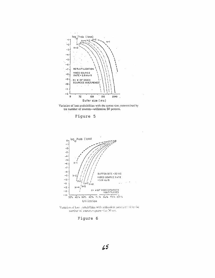
Figure 5

Figure 6

BIBLIOGRAPHY

[1] B. Maglaris, D. Anastassiou, P. Sen, G.Karlsson and J. Robbins, "Performance

models of statistical multiplexing in packet video communications,"IEEE Trans.

Commun., vol 36, pp 834-844, July 1988.

[2] J.S. Turner and L.F. Waytt, "A packet network architecture for integrated ser-

vices," in Proc. GLOBECOM '83, San Diego, CA, pp 2.1.1-2.1.6, Dec 1983.

[3] B.G. Haskell, "Buffer and channel sharing by several interframe picturephone

coders," Bell Syst. Tech J., vol. 51, no. 1, pp 261-289, Jan. 1972.

[4] L. Zhang, "Designing a new architecture for packet switching communication

networks," IEEE Commun. Magz, vol. 25, no. 9, pp 5-12, Sept. 1987.

[5] D. Bertsekas and R. Gallager, Data Networks, Prentice Hall:1987.

[6] J.S. Turner, "Design of an integrated services packet network," IEEE J. Select.

Areas Commun., vol. SAC-4, no.8, pp 1373-1380, Nov. 1986.

[7] L. Kleinrock, Queueing Systems, Vol 1, Vol 2. New York:Wiley, 1975 & 1976.

[8] A. Papoulis, Probability, Random Variables, and Stochastic Processes.

New York: McGraw Hill, 1984.

[9] W. Verbiest, "Video coding in an ATD environment," Proc. Third Int. Conf.

66

New Syst. Services Telecommun., Nov, 1986.

[10] S.Cheung, S. Dimitriadis, W.J.Karplus, "Introduction to simulation using Net-

work 11.5," CACI Products Company, 1988.

[11] Network 11.5 Users Manual, Version 4.0, CACI Products Company, 1988.

67