copyright warning &...
TRANSCRIPT
Copyright Warning & Restrictions
The copyright law of the United States (Title 17, United States Code) governs the making of photocopies or other
reproductions of copyrighted material.
Under certain conditions specified in the law, libraries and archives are authorized to furnish a photocopy or other
reproduction. One of these specified conditions is that the photocopy or reproduction is not to be “used for any
purpose other than private study, scholarship, or research.” If a, user makes a request for, or later uses, a photocopy or reproduction for purposes in excess of “fair use” that user
may be liable for copyright infringement,
This institution reserves the right to refuse to accept a copying order if, in its judgment, fulfillment of the order
would involve violation of copyright law.
Please Note: The author retains the copyright while the New Jersey Institute of Technology reserves the right to
distribute this thesis or dissertation
Printing note: If you do not wish to print this page, then select “Pages from: first page # to: last page #” on the print dialog screen
The Van Houten library has removed some of the personal information and all signatures from the approval page and biographical sketches of theses and dissertations in order to protect the identity of NJIT graduates and faculty.

ABSTRACT
THE MECHANICAL TESTING OF SINGLE NANOFIBER
by
Pratik Manohar Dahule
Polymer nanofibers exhibit properties that make them a favorable material for the
development of tissue engineering scaffolds, filtration devices, sensors, and high strength
lightweight materials. Perfectly aligned PLLA Nanofibers were fabricated by an
electrospinning technique under optimum conditions and the diameter of the electrospun
fibers can easily be tailored by adjusting the concentration of the polymer solution. To
align the nanofibers, special arrangement was made in terms of two aluminum plates.
Good alignment of polymer nanofibers on specimen was confirmed by SEM observation.
The effect of different electro-spinning parameters on maximum fiber length, average
fiber diameter, diameter uniformity, and fiber quality was explored in this study. The
force applied on the nanofiber was measured with the help of AFM by satisfying Hooke’s
Law. The elastic properties of PLLA nanofiber were investigated with the atomic force
microscope (AFM). The elasticity was calculated by analyzing the recorded force curves
with the help of the Hertz model. Mechanical testing confirmed that the single aligned
nanofiber can be an advancement in the commercial applications of nanofibers.
THE MECHANICAL TESTING OF SINGLE NANOFIBER
by
Pratik Manohar Dahule
ThesisSubmitted to the Faculty of
New Jersey Institute of TechnologyIn Partial Fulfillment of the Requirements for the Degree of
Master of Science in Mechanical Engineering
Department of Mechanical Engineering
January 2012

APPROVAL PAGE
THE MECHANICAL TESTING OF SINGLE NANOFIBER
Pratik Manohar Dahule
Dr. Michael Jaffe, Thesis Advisor DateResearch Professor of Biomedical Engineering, NJIT
Dr. Kwabena A Narh, Co Advisor DateProfessor of Mechanical Engineering, NJIT
Dr. Bryan Pfister, Committee Member DateAssociate Professor of Biomedical Engineering, NJIT
Dr. George Collins, Committee Member DateResearch Professor of Biomedical Engineering, NJIT
BIOGRAPHICAL SKETCH
Author: Pratik Manohar Dahule
Degree: Master of Science
Date: January 2012
Undergraduate and Graduate Education:
• Master of Science in Mechanical Engineering,New Jersey Institute of Technology, Newark, NJ, 2012
• Bachelor of Science in Mechanical Engineering,Amravati University, Pusad, India, 2009
Major: Mechanical Engineering
“Aum Shri GuruDev Dutt”
This thesis is dedicated to my father and mother who always stood behind me and gave
me so much of support every time. I am thankful to all my family, teachers and friends
who made me capable of reaching this point.
ACKNOWLEDGMENT
I would like to thank Dr. Michael Jaffe for not only being my advisor but also a guardian
who gave me good advices during my thesis and curriculum. I also express my gratitude
to Dr. George Collins who guided me with my research work. I would like to thank Dr.
Kwabena Narh and Dr. Bryan Pfister for being my committee members and showing
interest in my thesis. I am grateful to Ms. Xueyan Zhang for guiding and training me in
characterization technique, without which this research work would not have been
possible.
Last, but not the least, I would like to thank my family and my friends, Tanmay
Pathre, Harshil Poojara, Sampath, Arun, Anil Shrirao, Abhishek Bhagwat, Samarth
Trivedi, Tamil, Pranav Dahule, Mukul Bapat, Sandeep Singh, Pritam and others who
diligently helped me throughout my research work.
vi

TABLE OF CONTENTS
Chapter Page
1 INTRODUCTION 1
2 BACKGROUND 5
2.1 Electrospinning History. . 5
2.2 The Electrospinning Process 8
2.2.1 Electrospinning Technology: Current Scenario 10
2.2.2 Spinning of Polymeric Nanofibers .. 11
2.2.3 Structure and Morphology of Polymeric Nano-fibers .. 12
2.2.4 Process Parameters and Fiber Morphology 13
2.3 Common Biodegradable Polymers Used In Electrospinning 17
2.3.1 Poly (lactides) 17
2.4 Clinical and Industrial Applications of Nanofiber 19
2.4.1 Medical Prostheses 19
2.4.2 Tissue Engineering 19
2.4.3 Wound Dressing 20
2.4.4 Drug Delivery and Pharmaceutical Composition . 21
2.4.5 Filtration 21
2.5 Characterization of Nanofiber 23
3 RESEARCH OBJECTIVE 26
4 EXPERIMENTAL DESIGN 27
4.1 Electrospinning Equipment 27
vii
TABLE OF CONTENTS(Continued)
Chapter Page
4.2 Materials . 29
4.3 Solution Preparation 30
4.4 Characterization of Electro-spun Nano-fiber 31
4.4.1 Morphology 31
4.5 Mechanical Properties . 34
4.5.1 AFM Development & Principle of Operation 35
4.5.2 Modes of operation for the AFM 37
4.5.2 Atomic Force Microscope Operation 40
4.5.3 Forces Affecting AFM Probe 41
4.5.4 Measuring the Elastic Properties with the AFM 42
4.5.5 Assumptions and Challenges 43
4.5.6 Tip and Cantilever Selection and Tip Functionalization 45
5 RESULTS .. 47
5.1 Morphology of Electrospun Nanofiber 47
5.2 Mechanical Characterization of Electrospun Nanofiber . 49
5.3 Force Calibration Plot 51
6 DISCUSSION 55
7 CONCLUSIONS 57
8 FUTURE SCOPE OF RESEARCH . 58
9 REFERENCES 59
viii
LIST OF TABLES
Table Page
2.1 Common Properties of Poly (Lactic Acid) 18
ix
LIST OF FIGURES
Figures Page
4.1 Diagrammatic representation of electrospinning equipment 28
4.2 Schematic of the Operation of a SEM 32
4.3 LEO 1530 Field Emission SEM 33
4.4 Scheme of an atomic force microscope and the force-distance curvecharacteristic of the interaction between the tip and sample 35
4.5 Schematic diagram of optical changes in the deflection of the cantilever and aquadrant photodiode 36
4.6 Scheme of contact mode imaging and an image of cholera oligomers by Shao(U. Virginia) 37
4.7 Scheme of lateral force imaging and a friction image of self-assembledmonolayers on gold. The white regions terminate in –COOH, and the grayregions terminate in –CH 3 ; the tip is also functionalized with –COOH. C.M Lieber, Langmuir 14,1508 (1998) 38
4.8 Scheme of Tapping mode imaging and an image of DNA by B. Stine(Northwestern) 39
4.9 Scheme of non-contact mode imaging and an image of raspberry” polymers, DI. 40
4.10 Atomic Force Microscope schematic Diagram with components 41
5.1 SEM Image of Single Nanofiber obtained with 5% polymer concentration . 47
5.2 SEM Image of Parallel Aligned Nanofiber obtained with 6% polymerconcentration .. 47
5.3 SEM Image of Aligned Nanofiber obtained with 6% polymer concentration 48
5.4 SEM Image of Aligned Fiber obtained with 5% polymer concentration .. 48
5.5 Bar Graph Representation of Polymer Concentration Vs Fiber Diameter 49
5.6 AFM Image of Parallel Aligned Nanofiber obtained with 5% polymerconcentration . 50
x
LIST OF FIGURES(Continued)
Figures Page
5.7 AFM image of single nanofiber obtained with 5% polymerconcentration 50
5.8 Force curve obtained from interaction between cantilever tip and the nanofibersample 51
xi
CHAPTER 1
INTRODUCTION
Nanotechnology is the study of manipulating matter on an atomic and molecular scale.
Generally, nanotechnology deals with developing materials, devices, or other structures
possessing at least one dimension sized from 1 to 100 nanometers. Nanotechnology is the
science and engineering of creating materials, functional structures and devices on a
nanometer scale, corresponding to a length of 10 -9 m. The fascination of downsizing
materials to nanoscale dimensions comes from scientific observations of considerable
change in fundamental mechanical, physical, chemical and biological properties as a
function of their size, shape, surface chemistry and topology. Therefore, nanotechnology
has generated growing interest in the scientific community, and it has become a very
active area of research.
A polymeric fiber is a polymer whose aspect ratio is greater than 100. The
production of fibers from organic polymers involves forming the polymer into filaments
and extending them uniaxially in order to orient molecules in the direction of the applied
strain [1]. Conventional methods of polymer fiber production include melt spinning,
solution spinning and gel state spinning. These methods rely on mechanical forces to
produce fibers by extruding polymer melt or solution through a spinneret and
subsequently drawing the resulting filaments as they solidify or coagulate. By using these
methods, typical fiber diameters in the range of 5 to 500 microns can be produced. The
consistently producible minimum fiber diameter is on the order of a micron [2].
1
Though there are many methods of fiber production, Electrospinning is a much
reported, but to date minimally commercialized process to generate smaller fibers.
Electrospinning was first patented in 1897 and used in the textile industry in the 1930s
[3]. Electrospinning is a unique method that produces polymer fibers with diameter in the
range of nanometer to a few microns using electrically driven jet of polymer solution or
melt [4, 5]. This technique has been developed since introduced by Formhals in 1934 [3].
It did not gain significant industrial importance in the past due to the low output of the
process, inconsistent and low molecular orientation, poor mechanical properties and high
diameter distribution of the electrospun fibers. The electrospinning process itself begins
with a solution of polymers, long chains of molecules, pumped into an electrified metal
nozzle. High voltage creates a cone of fluid outside the nozzle, and a tiny jet of material
erupts, electrically attracted to a target surface a few inches below the nozzle. In a few
milliseconds, the electric field aligns the polymer molecules in the jet stream into fibrous
strands, pulling and stretching the jet 1,000 times thinner than the micron-sized nozzle
opening, to about diameters in the nanometer range [3].
Electrospun fibers have nanostructured surface morphologies with tiny pores that
influence mechanical property like Young’s modulus . As it is evident, there is less
information available on the mechanical properties of nano fibers. Research on the
mechanical properties of nanofibers from a variety of polymers is essential for a greater
understanding on the contributions of nanofibers to the mechanical and performance
related characteristics of nano fiber. Nanofibers have been attracting the attention of
global materials research these days primarily due to their enhanced properties required
for application in specific areas like catalysis, filtration, nano electro-mechanical system
3
(HEMS), nanocomposites, nano fibrous structures, tissue scaffolds, drug delivery systems,
protective textiles, storage cells for hydrogen fuel cells, etc. Carbon nano fibers are
finding enormous applications in unconventional energy sources and storage cells, due to
their enhanced conductivity and high aspect ratio. Their mechanical properties enable
them to be used as fillers in composites that find applications in synthetic and rubber
industries. Carbon nanofiber reinforced composites offer increased stiffness, high
strength and low electrical resistivity. Also, aligned nano fiber composites provide
enhanced mechanical properties than the randomly aligned nano fiber composite structure.
The electrospun nanofibers provide a very large surface area/mass due to their
small diameter, hence non-woven fabrics, with small fibers can be used for filtration of
sub-particles in the separation industry. These can also be used for the adsorption of
biological and chemical warfare gases, protective clothing, in medical industry as
artificial blood vessels, sutures, surgical facemask, fiber-reinforced materials,
monodirectional composites and in agricultural field for control of pesticides. The
electrospinning technique can be used in chemical and manufacturing industries for paint
spraying, electro deposition, plasma deposition, and mining minerals. In general, polymer
nanofibers are used in a variety of applications, including filtration, protective clothing,
biomedical applications such as wound dressing and drug delivery systems, design of
solar cells, light cells and mirrors for use in space, as well as for structural elements in
artificial organs and in reinforced composites. Ceramic or carbon nanofibers made from
polymer precursors make it possible to expand the list of possible uses for nanofibers.
Another promising field of application of nanofibers is tissue engineering. Synthetic
tissues help stimulate living tissues to repair themselves in various parts of the human
4
body, such as cartilage, blood vessels, bones and so forth, due to diseases or wear and
tear. Victims whose skin are burned or scalded by fire or boiling water may also find an
answer in synthetic tissues. The newest generation of synthetic implant materials, also
called biomaterials, may even treat diseases such as Parkinson's, arthritis and
osteoporosis.
In this study, nanofiber was produced by electrospinning poly L (lactides), their
morphology was characterized with the help of Scanning Electron Microscope and
mechanical characterization was done with the help of Atomic Force Microscope.
CHAPTER 2
BACKGROUND
A number of processing techniques such as drawing, template synthesis, phase
separation, self-assembly, electrospinning have been used to prepare polymer nanofibers
in recent years. According to Zheng-Ming Huang [6] the electrospinning process is the
only method, which can be further developed for mass production of one-by-one
continuous nanofibers from various polymers. Despite possessing these unique features,
one of the main challenges in this area is to characterize the mechanical behavior of the
nanofibers. This could be due to the difficulty in handling the nano fibers and also due to
the low load required for the deformation. Hence, in most cases, the mechanical integrity
of the fibers is least understood and an understanding of the phenomenon is urgently
needed. In most of the applications, the nanofibers are subjected to stresses and strains
from surrounding media during their service lifetime. Such stresses can cause permanent
deformation and even failure to the nanofibers. Therefore there is a need to characterize
the mechanical properties of nanofiber [7].
2.1 Electrospinning History
The electrostatic spray literature contains many helpful insights into the electrospinning
process. Lord Raleigh [8] studied the instabilities that occur in electrically charged liquid
droplets. He showed, over 100 years ago, that when the electrostatic force overcame the
surface tension, a liquid jet was created. Zeleny [9] considered the role of surface
instabilities in electrical discharges from drops. He published a series of papers around
5
6
1910 on discharges from charged drops falling in electric fields, and showed that, when
the discharge began, the theoretical relations for the surface instability were satisfied. In
1952, Vonnegut and Neubaur [10] produced uniform streams of highly charged droplets
with diameters of around 0.1mm, by applying potentials of 5 to 10 kilovolts to liquids
flowing from capillary tubes. Their experiment proved that monodisperse aerosols with a
particle radius of a micron or less could be formed from pendent droplet at the end of the
pipette. The diameter of the droplet was sensitive to the applied potential. Wachtel and
coworkers [11] prepared emulsion particles using 45 electrostatic methods to make a
monodisperse emulsion of oil in water. The diameters of the emulsion particles were
from 0.5 to 1.6 microns. In 1960's Taylor [12] studied the disintegration of water droplets
in an electric field. His theoretical papers demonstrated that a conical interface, with a
semi-angle close to 49.3°, was the limiting stable shape.
Gladding [13] and Simons [14] improved the electrospinning apparatus and
produced more stable fibers. They used movable devices such as a continuous belt for
collecting the fibers. Later, Bornat [15] patented another electro-spinning apparatus that
produced a removable sheath on a rotating mandrel. The basic principles were similar to
previous patents. He determined that the tubular product obtained by electrospinning
polyurethane materials in this way could be used for synthetic blood vessels and urinary
ducts.
In 1971, electrospinning of acrylic fibers was described by Baumgarten [16].
Acrylic polymers were electrospun from dimethylformamide solution into fibers with
diameters less than 1 micron. A stainless steel capillary tube was used to suspend the
drop of polymer solution and the electrospun fibers were collected on a grounded metal
7
screen. Baumgarten observed relationships between fiber diameter, jet length, solution
viscosity, feed rate of the solution and the composition of the surrounding gas.
In 1981, Manley and Larrondo [17] reported that continuous fibers of
polyethylene and polypropylene could be electrospun from the melt, without mechanical
forces. A drop of molten polymer was formed at the end of a capillary. A molten polymer
jet was formed when high electric field was established at the surface of the polymer. The
jet became thinner and then solidified into a continuous fiber. The molecules in the fiber
were oriented by an amount similar to that found in conventional as-spun textile fibers
before being drawn. The fiber diameter depended on the electric field, the operating
temperature and the viscosity of the sample. X-ray diffraction and mechanical testing
characterized the electrospun fibers. As either the applied electric field or the take-up
velocity was increased, the diffraction rings became arcs, showing that the molecules
were elongated along the fiber axis.
Reneker and coworkers [18] made further contributions to understanding the
electro-spinning process and characterizing the electrospun nanofibers in recent years.
Doshi [19] made electrospun nanofibers, from water-soluble poly (ethylene oxide), with
diameters of .05 to 5 microns. He described the electrospinning process, the processing
conditions, fiber morphology and some possible uses of electrospun fibers. Srinivasan
[20] electro-spun a liquid crystal polyaramid, poly (p-phenylene terephthalamide), and an
electrically conducting polymer, poly(aniline), each from solution in sulfuric acid. He
observed electron diffraction patterns of polyaramid nanofibers both as spun and after
annealing at 400°C. Chun [21] used transmission electron microscopy, scanning electron
microscopy and atomic force microscopy to characterize electrospun fibers of poly
8
(ethylene terephthalate). Fang [22] electrospun DNA into nanofibers, some of which
were beaded.
2.2 The Electrospinning Process
Electrospinning is a unique approach using electrostatic forces to produce fine fibers.
Electrostatic precipitators and pesticide sprayers are some of the well known applications
that work similarly to the electrospinning technique. Fiber production using electrostatic
forces has invoked glare and attention due to its potential to form fine fibers. Electrospun
fibers have small pore size and high surface area. There is also evidence of sizable static
charges in electrospun fibers that could be effectively handled to produce three
dimensional structures [23].
According to the authors of article [21], electrospinning is a process by which a
polymer solution or melt can be spun into smaller diameter fibers using a high potential
electric field. This generic description is appropriate as it covers a wide range of fibers
with submicron diameters that are normally produced by electrospinning. Based on
earlier research results, it is evident that the average diameter of electrospun fibers ranges
from 100 nm–500 nm. In textile and fiber science related scientific literature, fibers with
diameters in the range 100 nm–500 nm are generally referred to as nano fibers. The
advantages of the electrospinning process are its technical simplicity and its easy
adaptability. The apparatus used for electrospinning is simple in construction, which
consists of a high voltage electric source with positive or negative polarity, a syringe
pump with capillaries or tubes to carry the solution from the syringe or pipette to the
9
spinnerette, and a conducting collector like aluminum. The collector can be made of any
shape according to the requirements, like a flat plate, rotating drum, etc.
Polymer solution or the melt that has to be spun is forced through a syringe pump
to form a pendant drop of the polymer at the tip of the capillary. High voltage potential is
applied to the polymer solution inside the syringe through an immersed electrode, thereby
inducing free charges into the polymer solution. These charged ions move in response to
the applied electric field towards the electrode of opposite polarity, thereby transferring
tensile forces to the polymer liquid [21]. At the tip of the capillary, the pendant
hemispherical polymer drop takes a cone like projection in the presence of an electric
field. And, when the applied potential reaches a critical value required to overcome the
surface tension of the liquid, a jet of liquid is ejected from the cone tip [12].
Most charge carriers in organic solvents and polymers have lower mobilities, and
hence the charge is expected to move through the liquid for larger distances only if given
enough time. After the initiation from the cone, the jet undergoes a chaotic motion or
bending instability and is field directed towards the oppositively charged collector, which
collects the charged fibers [24]. As the jet travels through the atmosphere, the solvent
evaporates, leaving behind a dry fiber on the collecting device. For low viscosity
solutions, the jet breaks up into droplets, while for high viscosity solutions it travels to
the collector as fiber jets [25].
10
2.2.1 Electrospinning Technology: Current Scenario
There has been a substantial amount of research carried out on the fundamental aspects of
electrospinning. The major issue that is yet to be resolved is the scaling-up of the process
for commercialization. Academic and research communities should join hands in taking
the lab-scale technology to the commercial level. A succinct summary on nano fiber
research that is of use to the fiber and textile industry has been provided by Shastri and
Ramkumar [26].
Electrospinning apparatus is simple in construction, and there have been no
significant developments in the equipment design in the last decade. Research groups
have improvised the basic electrospinning setup to suit their experimental needs and
conditions. Warner et al. [27] have designed a new parallel plate setup for effectively
controlling the operating variables to quantify the electro hydrodynamics of the process.
The parallel plate design is expected to overcome the problem of a nonuniform electric
field experienced in the point plate configuration. Jaeger et al. have used a two electrode
setup by placing an additional ring electrode in front of the capillary to reduce the effect
of the electrostatic field at the tip and to avoid corona discharges [28]. It has been
stipulated that by using the two electrode setup, a more stable field can be established
between the ring electrode and the collector, thereby avoiding the effect of changing
shape at the capillary tip over the electric field.
Productivity enhancement for commercializing the electrospinning process is
under active research, with emphasis on multiple spinneret designs and alternative
experimental setup for feed charging. However, there is still a debate on the potential of
11
scaling up this technology for commercialization. There are only a few technology
companies engaged in research and development on nano fibers. There is hardly any
information available in the public domain on the mass production of nanofibers for
different applications. Espin Technologies, a nanofiber technology company, is involved
in developing a proprietary high speed device that could effectively overcome the
traditional drawbacks of low output and high production cost [29].
Donaldson filtration Company has its own patented process setup for making tens
of thousands of square meters of electrospun nano fiber filter media [30]. From the
available published literature and the current state of understanding of the electrospinning
process, it is likely that commercial scaling up of the electrospinning process can only be
achieved by more fundamental understanding of the process and better control of the
instability behavior of the jets that determine the diameter of the fibers. In addition, there
needs to be an active participation between government agencies, industry, and academia
for scaling-up the process. With greater enthusiasm among the interested parties,
programs that are in place, such as Grants Opportunities for Academic Liaison with
Industry of the NSF and SBIR programs, can be of assistance for technology transfer and
commercialization.
2.2.2 Spinning of Polymeric Nanofibers
Research activity on the electrospinning of nanofibers has been successful in spinning
submicron range fibers from different polymeric solutions and melts. Although a plethora
of literature is available on the structure and morphological properties of polymeric
nanofibers, there is very little information in the public domain on the electro
12
hydrodynamics of the electrospinning process. Polymers with attractive chemical,
mechanical, and electrical properties like high conductivity, high chemical resistance, and
high tensile strength have been spun into ultra fine fibers by the electrospinning process,
and their application potential in areas like filtration, optical fibers, drug delivery system,
tissue scaffolds, and protective textiles have been examined [25, 31].
2.2.3 Structure and Morphology of Polymeric Nano-fibers
In recent times, nanofibers have attracted the attention of researchers due to their
pronounced micro and nano structural characteristics that enable the development of
advanced materials that have sophisticated applications. More importantly, high surface
area, small pore size, and the possibility of producing three dimensional structures have
increased the interest in nanofibers. As theoretical studies on the electrospinning process
have been conducted by various groups [24, 32-38] for a while to understand the
electrospinning process, there have been some simultaneous efforts to characterize the
structure and morphology of nano fibers as a function of process parameters and material
characteristics.
The production of nanofibers by the electro-spinning process is influenced both by
the electrostatic forces and the viscoelastic behavior of the polymer. Process parameters,
like solution feed rate, applied voltage, nozzle-collector distance, and spinning
environment, and material properties, like solution concentration, viscosity, surface
tension, conductivity, and solvent vapor pressure, in fluence the structure and properties of
electrospun nanofibers. Significant work has been done to characterize the properties of
fibers as a function of process and material parameters. A detailed account on the
13
influence of process and material characteristics on the structure and properties of
nanofibers is provided in the following sections of this paper.
2.2.4 Process Parameters and Fiber Morphology
Applied voltage
Various instability modes that occur during the fiber forming process are expected to
occur by the combined effect of both the electrostatic field and the material properties of
the polymer. It has been suggested that the onset of different modes of instabilities in the
electrospinning process depend on the shape of the jet initiating surface and the degree of
instability, which effectively produces changes in the fiber morphology [25]. In
electrospinning, the charge transport due to the applied voltage is mainly due to the flow
of the polymer jet towards the collector, and the increase or decrease in the current is
attributed to the mass flow of the polymer from the nozzle tip. Deitzel et al. have inferred
that the change in the spinning current is related to the change in the instability mode
[25]. They experimentally showed that an increase in applied voltage causes a change in
the shape of the jet initiating point, and hence the structure and morphology of fibers.
Experimentation on a PEO/water system has shown an increase in the spinning current
with an increase in the voltage [25].
It was also observed that for the PEO/water system, the fiber morphology changed
from a defect free fiber at an initiating voltage of 5.5 kV to a highly beaded structure at a
voltage of 9.0 kV [25]. The occurrence of beaded morphology has been correlated to a
steep increase in the spinning current, which controls the bead formation in the

14
electrospinning process. Beaded structure reduces the surface area, which ultimately
influence the filtration abilities of nanofibers.
Earlier in 1971, Baumgarten while carrying out experiments with acrylic fibers
observed an increase in fiber length of approximately twice with small changes in fiber
diameter with an increase in applied voltage [16]. Megelski et al. [39] investigated the
voltage dependence on the fiber diameter using polystyrene (PS). The PS fiber size
decreased from about 20 m to 10 m with an increase in voltage from 5 kV to 12 kV,
while there was no significant change observed in the pore size distribution. These results
concur with the interpretation of Buchko et al., [40] who observed a decrease in the fiber
diameter with an increase in the applied field while spinning silk like polymer fiber with
fibronectin functionality (SLPF). Generally, it has been accepted that an increase in the
applied voltage increases the deposition rate due to higher mass flow from the needle tip.
Jaeger et al. used a two-electrode setup for electrospinning by introducing a ring
electrode in between the nozzle and the collector [28]. The ring electrode was set at the
same potential as the electrode immersed in the polymer solution. This setup was thought
to produce a field-free space at the nozzle tip to avoid changes in the shape of the jet
initiating surface due to varied potential [28]. Though this setup reduces the unstable jet
behavior at the initiation stage, bending instability is still dominant at later stages of the
process, causing an uneven chaotic motion of the jet before depositing itself as a
nonwoven matrix on the collector. Deitzel et al. experimented with a new electrospinning
apparatus by introducing eight copper rings in series in between the nozzle and the
collector for dampening the bending instability [41].

15
The nozzle and the ring set were subjected to different potentials (ring set at a
lower potential) of positive polarity, while the collector was subjected to a negative
polarity. The idea behind this setup was to change the shape of the macroscopic electric
field from the jet initiation to the collection target in s uch a way that the field lines
converge to a center line above the collection target by the applied potential to the ring
electrodes. The authors have suggested that the bending instability of fibers was
dampened by the effect of the converging field lines producing straight jets [41].
Controlled deposition helps to produce speci fic deposition patterns and also yarn like
fibers. Deitzel et al. investigated the spinning of PEO in aqueous solution using multiple
electric fields, which resulted in fibers depositing over a reduced area due to the
dampening of bending instability. The multiple field technique was also shown to
produce fibers of lesser diameter than the conventional electrospinning method [41].
Nozzle collector distance
The structure and morphology of electrospun fibers is easily affected by the nozzle to
collector distance because of their dependence on the deposition time, evaporation rate,
and whipping or instability interval. Buchko et al. examined the morphological changes
in SLPF and nylon electrospun fibers with variations in the distance between the nozzle
and the collector screen. They showed that regardless of the concentration of the solution,
lesser nozzle-collector distance produces wet fibers and beaded structures. SLPF fiber
morphology changed from round to flat shape with a decrease in the nozzle collector
distance from 2cm to 0.5cm [40]. This result shows the effect of the nozzle collector
distance on fiber morphology. The work also showed that aqueous polymer solutions
require more distance for dry fiber formation than systems that use highly volatile organic

16
solvents [40]. Megelski et al. observed bead formation in electrospun PS fibers on
reducing the nozzle to collector distance, while preserving the ribbon shaped morphology
with a decrease in the nozzle to collector distance [39].
Polymer flow rate
The flow rate of the polymer from the syringe is an important process parameter as it
influences the jet velocity and the material transfer rate. In the case of PS fibers, Megelski
et al. observed that the fiber diameter and the pore diameter increased with an increase in
the polymer flow rate [39]. As the flow rate increased, fibers had pronounced beaded
morphologies and the mean pore size increased from 90 to 150 nm [39].
Spinning environment
Environmental conditions around the spinneret, like the surrounding air, its relative
humidity (RH), vacuum conditions, surrounding gas, etc., influence the fiber structure and
morphology of electrospun fibers. Baumgarden observed that acrylic fibers spun in an
atmosphere of relative humidity more than 60% do not dry properly and get entangled on
the surface of the collector [16]. The breakdown voltage of the atmospheric gases is said
to influence the charge retaining capacity of the fibers [16]. Megelski et al. investigated
the pore characteristics of PS fibers at varied RH and emphasized the importance of phase
separation mechanisms in explaining the pore formation of electrospun fibers [39].
17
2.3 Common Biodegradable Polymers Used In Electrospinning
Biodegradable polymers can be either natural or synthetic. In general, synthetic polymers
offer greater advantages than natural materials because they can be tailored to give a
wider range of properties and more predictable uniformity than can materials from
natural sources. Synthetic polymers also represent a more reliable source of raw
materials, one free from concerns of immunogenicity.
2.3.1 Poly (lactides)
Poly (Lactic Acid) 4 (--CO---CH (CH3)--O--)n
Poly (Glycolic Acid) 4 (--CO--CH2--O--)n
Poly (Lactic Acid-co- Glycolic Acid) 4
(--CO---CH (CH3)--O--)x-- (--CO--CH2)y--COOH
Poly (glycolic) acid (PGA) and poly (lactic acid) (PLA) are aliphatic polyesters of poly( a
hydroxy acids). These polymers and their associated copolymers are perhaps the most
common biodegradable synthetic polymers known and have been used in drug delivery,
bone osteosynthesis and tissue engineering of skin [42]. PGA's relatively short chain
length and polar properties give rise to its high crystallinity, melting point and low
solubility in organic solvents [42]. PGA is also insoluble in the organic chloroform and
dioxane solvents used in creating the scaffolds. This project is therefore unable to explore
PGA polymer nonwoven webs.
As seen in the structures above, PLA has an extra chiral methyl group, making a
D- or L- isomer possible. This extra methyl group also makes PLA more hydrophobic
18
than PGA. PLA is hydrophobic and films of PLA take up only about 2% water [42]. Due
to steric hindrance of the methyl group, the ester bond of PLA is less likely to undergo
hydrolysis, making the degradation time for PLA longer than its relative PGA and its
copolymer PLGA. Other factors such as molecular weight, exposed surface area and
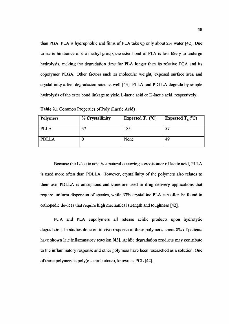
crystallinity affect degradation rates as well [43]. PLLA and PDLLA degrade by simple
hydrolysis of the ester bond linkage to yield L-lactic acid or D-lactic acid, respectively.
Table 2.1 Common Properties of Poly (Lactic Acid)
Polymers % Crystallinity Expected Tm (oC) Expected T g (oC)
PLLA 37 185 57
PDLLA 0 None 49
Because the L-lactic acid is a natural occurring stereoisomer of lactic acid, PLLA
is used more often than PDLLA. However, crystallinity of the polymers also relates to
their use. PDLLA is amorphous and therefore used in drug delivery applications that
require uniform dispersion of species, while 37% crystalline PLA can often be found in
orthopedic devices that require high mechanical strength and toughness [42].
PGA and PLA copolymers all release acidic products upon hydrolytic
degradation. In studies done on in vivo response of these polymers, about 8% of patients
have shown late inflammatory reaction [43]. Acidic degradation products may contribute
to the inflammatory response and other polymers have been researched as a solution. One
of these polymers is poly(s-caprolactone), known as PCL [42].
19
2.4 Clinical and Industrial Applications of Nanofibers
From a biological viewpoint, almost all of the human tissues and organs are deposited in
nano fibrous forms or structures. Examples include: bone, dentin, collagen, cartilage, and
skin. All of them are characterized by well-organized hierarchical fibrous structures14
realigning in nanometer scale. According to the research conducted in the field of
nanotechnology, compatibility has to do with the size of the fibers that make up the
materials. As such, current research in electrospun polymer nanofibers has focused one of
their major applications on bioengineering.
2.4.1 Medical Prostheses
Polymer nanofibers fabricated via electrospinning have been proposed for a number of
soft tissue prostheses applications such as blood vessel, vascular, breast, etc. In addition,
electrospun biocompatible polymer nanofibers can also be deposited as a thin porous film
onto a hard tissue prosthetic device designed to be implanted into the human body. This
coating film with gradient fibrous structure works as an interphase between the prosthetic
device and the host tissues, and is expected to efficiently reduce the stiffness mismatch at
tissue/device interphase and hence prevent the device failure after the implantation [44].
2.4.2 Tissue Engineering
For the treatment of tissues or organs in malfunction in a human body, one of the
challenges to the field of tissue engineering is the design of ideal scaffolds/synthetic
matrices that can mimic the structure and biological functions of the natural extracellular
matrix (ECM). Human cells can attach and organize well around fibers with diameters
smaller than those of the cells. In this regard, nanoscale fibrous scaffolds can provide an

20
optimal template for cells to seed, migrate, and grow. A successful regeneration of
biological tissues and organs calls for the development of fibrous structures with fiber
architectures beneficial for cell deposition and cell proliferation. Of particular interest in
tissue engineering is the creation of reproducible and biocompatible three-dimensional
scaffolds for cell ingrowths resulting in bio-matrix composites for various tissue repair
and replacement procedures. Recently, people have started to pay attention to making
such scaffolds with synthetic biodegradable polymer nanofibers. It is believed that
converting biopolymers into fibers and networks that mimic native structures will
ultimately enhance the utility of these materials, as large diameter fibers do not mimic the
morphological characteristics of the native fibrils [44].
2.4.3 Wound Dressing
Polymer nanofibers can also be used for the treatment of wounds or bums of a human
skin, as well as designed for haemostatic devices with some unique characteristics. With
the aid of electric field, fine fibers of biodegradable polymers can be directly
sprayed/spun onto the injured location of skin to form a fibrous mat dressing which can
let wounds heal by encouraging the formation of normal skin growth and eliminate the
formation of scar tissue, which would occur in a traditional treatment. Non-woven
nanofibrous membrane mats for wound dressing usually have pore sizes ranging from
500 nm to 1 mm, small enough to protect the wound from bacterial penetration via
aerosol particle capturing mechanisms. High surface area of 5-100 m 2/g is extremely
efficient for fluid absorption and dermal delivery [44].
21
2.4.4 Drug Delivery and Pharmaceutical Composition
Delivery of drug/pharmaceuticals to patients in the most physiologically acceptable
manner has always been an important concern in medicine. In general, the smaller the
dimensions of the drug and the coating material required to encapsulate the drug, the
better the drug to be absorbed by human being. Drug delivery with polymer nanofibers is
based on the principle that dissolution rate of a particulate drug increases with increasing
surface area of both the drug and the corresponding carrier if needed. As the drug and
carrier materials can be mixed together for electrospinning of nanofibers, the likely
modes of the drug in the resulting nano structured products are: (1) drug as particles
attached to the surface of the carrier which is in the form of nanofibers, (2) both drug and
carrier are nanofiber-form, hence the end product will be the two kinds of nanofibers
interlaced together, (3) the blend of drug and carrier materials integrated into one kind of
fibers containing both components, and (4) the carrier material is electrospun into a
tubular form in which the drug particles are encapsulated. The modes (3) and (4) are
preferred. However, as the drug delivery in the form of nanofibers is still in the early
stage exploration, a real delivery mode after production and efficiency have yet to be
determined in the future [44].
2.4.5 Filtration
Polymeric nanofibers have been used in air filtration applications for more than a decade
[45]. Due to poor mechanical properties of thin nanowebs, they were laid over a substrate
suitable enough to be made into a filtration medium. The small fibe r diameters cause slip
flow at fiber surfaces, causing an increase in the interception and inertial impaction
22
efficiencies of these composite filter media [46]. The enhanced filtration efficiency at the
same pressure drop is possible with fibers having diameters less than 0.5 micron [46].
The potential for using nano fiber webs as a filtering medium is highly promising.
Knowing that the essential properties of protective clothing are high moisture vapor
transport, increased fabric breathability, and enhanced toxic chemical resistance,
electrospun nanofiber membranes have been found to be good candidates for these
applications [47]. The highly porous electrospun membrane surfaces help in moisture
vapor transmission. Gibson et al. have analyzed the possibility of using thin nano fiber
layers over the conventionally used nonwoven filtration media for protective clothing
[48]. Polyurethane and nylon nanowebs were applied over open cell foams and carbon
beads and tested for air flow resistance. They concluded that the airflow r esistance,
filtration efficiency, and pore sizes of nonwoven filter media could be easily altered by
coating with the lightweight electrospun nanofibers [48]. Doshi et al. have evaluated
composites of nanofibers with spunbond and melt blown fabrics for filtrati on
characteristics [49]. The nano fiber composite membranes have shown very high increase
in the filtration efficiencies [49]. Researchers at General Motors Company are working
on nanofibers for different composite applications because of its scratch/ wear res istance,
low temperature ductility, low flammability, and recyclability [50].
Nanofibers also find applications in aerospace and semiconductor industries.
Piezoelectric polymers were electrospun and investigated for applicability as a
component on the wings of micro-air vehicles [51 ].
23
2.5 Characterization of Nanofibers
Although the concept the electrospinning dates back to many years from now, not much
of characterization has been done in this field. The demand of these electrospun fibers in
wide variety of applications has influenced to develop the characterization and testing
techniques for the nanofibers produced.
One of the foremost roles of the electrospinning process is to produce small
diameter fibers. Almost everybody who has done electrospinning experiments has
reported that the fibers spun through this process have fiber diameters in the range of a
few nanometers to a couple of microns. Fibers spun through different polymer solutions
did not make much of a difference in the fiber diameter. The measurement of fiber
diameter in the electrospun webs that have been reported in the literature is based using
various image analysis techniques. The instruments for measuring the fiber diameter and
the analysis have been done using various instruments, mainly scanning electron
microscope, transmission electron microscope and atomic force microscopes.
There is very little data available in the literature on the mechanical properties of
electrospun nonwoven mats because not much work is done in this field [52]. It has been
supposed that nanofibers can have better mechanical performance than microfibers [44].
Till now in the open literature no one has given information in detail regarding their
mechanical properties and how the electrospinning process parameters affect their
properties.
During the service lifetime of the nano fibers, forces exerted on the fibers in the
form of mechanical contact or thermal misfit may result in permanent deformation or

24
even failure. Therefore, there is a need to characterize the mechanical properties of single
nanofibers. Commercial mechanical testing systems have been used to test fibers as small
as about 10 µm in diameter [53]. However, as the size of the fibers is further reduced,
such mechanical testing systems are not suitable for testing these ultra fine fibers due to
the following challenges:
1. Manipulating extremely small fibers. Due to the small size of the nanofibers,handling these fibers without damaging them can be very challenging. Custommade [54] and commercial [55] micro-manipulation systems can be used tomove the fibers and attach the fiber ends to grips or fixtures. However, suchsystems may not be suitable for certain types of nano fibers as will beexplained next.
2. Finding suitable mode of observation. Most of the manipulation systems aremore suitable for operation under scanning electron microscopes (SEM) sincethe magnification of optical microscopes is insufficient for observingnanofibers in the lower nanometer range (<250 nm). This limits the use of themanipulation systems to conductive samples such as carbon nanotubes. Non-conductive samples such as polymers may be damaged by the electron beamin the SEM. Similarly, mechanical tests can be carried out in SEM [54] andtransmission electron microscope (TEM) [56] for conductive samples only.
3. Sourcing for accurate and sensitive force transducer. The load resolution ofmost commercial mechanical testing systems depends on the type of load cellused. The smallest load cell of such systems can achieve a load resolution of0.1 mN [57]. This resolution is insufficient for the testing of nano fibers sincethe force required to break them can be in the nano Newton range. Onecommercially available mechanical testing system that may now be suitablefor nanofibers with diameters in the range of hundreds of nanometers is theNanoBionix (MTS, USA). It has a load resolution of 50 nN.
4. Sourcing for accurate actuator with high resolution. The lengths of nano fiberscan range from a few micrometers for nanowires to a few centimeters forcontinuous electrospun fibers. An actuator with high resolution is especiallycrucial for short fibers since the fibers can break in less than one micrometerof deformation [58, 59].
25
5. Preparing samples of single-strand nano fibers. Single strand nanofibers haveto be prepared in order to obtain the mechanical properties of individualfibers. This may not be difficult if MEMS are used to stretch single strandsamples since they can be prepared using conventional micro fabricationmethods. However, if the nanofibers are fabricated in the form of a three-dimensional continuous network, isolating single fibers for mechanical testscan be difficult. One such example is a nano fibrous scaffold produced by thephase separation method [60].
A review of the mechanical characterization techniques has been developed to test
nanofibers by E.P.S. Tan, C.T. Lim. These techniques include tensile test, bend test and
indentation done at the nanoscale [7].
CHAPTER 3
RESEARCH OBJECTIVE
This thesis was divided into two parts because while working on part I in the process of
making aligned nanofiber, it was observed that to obtain single nanofiber is challenging
and if mechanical behavior of single nanofiber is indentified then it can be useful from
various aspect of applications. This led to part II of thesis for which characterization
technique was used to investigate mechanical properties.
The objective of first part of the thesis is to produce aligned nanofiber of poly L
lactic acid using electrospinning and properly obtain that specimen of single nanofiber to
study their mechanical behavior in biorelevant conditions.
The objective of second part of the thesis is to perform testing on single nanofiber
to investigate mechanical properties of single nanofiber using scanning electron
microscopy (SEM), atomic force microscopy (AFM).
26
CHAPTER 4
EXPERIMENTAL DESIGN
At the outset, this chapter gives a brief introduction about the description of the project and
discusses the materials which are utilized in this research to produce nanofiber. It explains
the methods that are used in this research to produce aligned nanofiber. This includes the
apparatus design and the typical electrospinning conditions that are used to get the aligned
nanofiber. Finally a brief description of the characterization procedure using Scanning
Electron Microscopy (SEM) and Atomic Force Microscopy (AFM) is given.
The mechanical properties of nanofibrous scaffold can affect cell morphology,
proliferation. In order to evaluate the mechanical behavior of scaffolds under various
loading conditions, it is necessary to obtain the mechanical properties of individual fibers
that make up the scaffold. So in order to use the fabricated nanofibers for mechanical tests,
an appropriate method is required for isolating and handling single nanofiber filament. In
order to meet the above requirements, the electrospinning apparatus was designed to guide
the electrospinning jet, which made possible to collect the electrospun nanofiber as
uniaxially aligned arrays.
4.1 Electrospinning Equipment
To achieve the research objectives, an electrospinning apparatus setup was designed and
constructed. The apparatus consists of two main devices, the sprayer and the collecting
device.
27
28
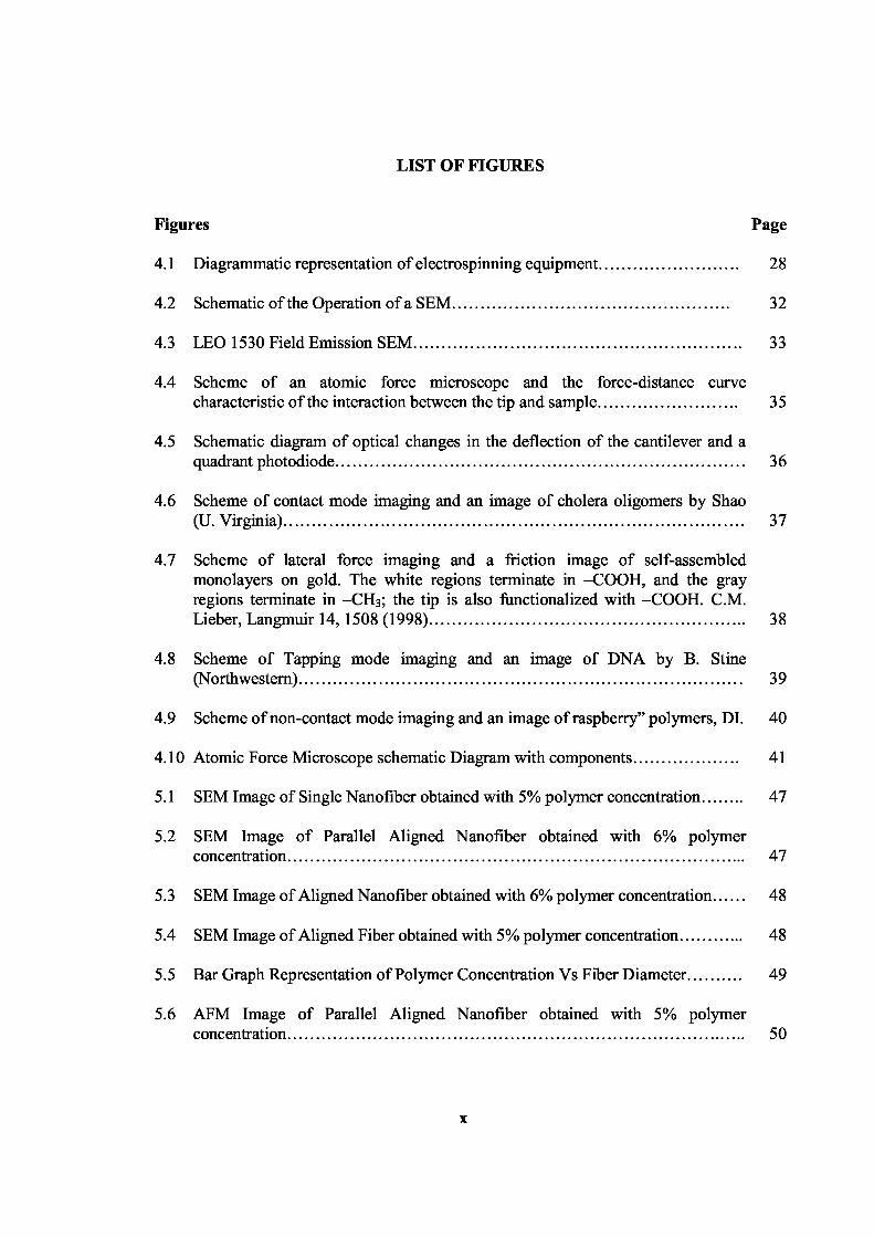
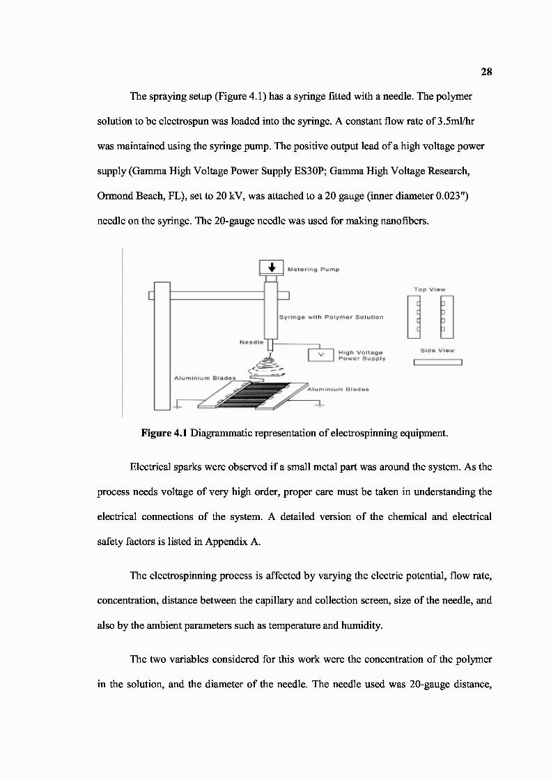
The spraying setup (Figure 4.1) has a syringe fitted with a needle. The polymer
solution to be electrospun was loaded into the syringe. A constant flow rate of 3.5ml/hr
was maintained using the syringe pump. The positive output lead of a high voltage power
supply (Gamma High Voltage Power Supply ES30P; Gamma High Voltage Research,
Ormond Beach, FL), set to 20 kV, was attached to a 20 gauge (inner diameter 0.023 ")
needle on the syringe. The 20-gauge needle was used for making nanofibers.
Figure 4.1 Diagrammatic representation of electrospinning equipment.
Electrical sparks were observed if a small metal part was around the system. As the
process needs voltage of very high order, proper care must be taken in understanding the
electrical connections of the system. A detailed version of the chemical and electrical
safety factors is listed in Appendix A.
The electrospinning process is affected by varying the electric potential, flow rate,
concentration, distance between the capillary and collection screen, size of the needle, and
also by the ambient parameters such as temperature and humidity.
The two variables considered for this work were the concentration of the polymer
in the solution, and the diameter of the needle. The needle used was 20-gauge distance,
29
wherein electric voltage is the applied voltage to the polymer solution and collecting
distance. The voltage used for the process was 20 kV. The collector to needle distance was
20 centimeters. For the fabrication of PLLA nanofibers, a 20-gauge needle was used for
spinning a solution of 5% w/w, 6% w/w concentration. After this, in order to assess the
mechanical properties of electrospun fibers, a single filament of nanofiber was obtained
with the technique of double sided tape suck on parallel plates which allows single
nanofiber to be isolated and handled. A method has been developed to isolate individual
electrospun fibers. The parallel arrangement of aluminum electrodes with a double sided
tape was attached to both the ends of the aluminum electrodes to facilitate the attachment
of fibers. The distance between the parallel strips was set to 1.2 cm to accommodate the
height of the frame.
The fibers were electrospun with a typical flow rate of 3.5 ml/hr and a potential
difference of 20 kV was applied. Electrospun process was carried out only for a few
seconds to get a few strands of fibers across the aluminum electrodes. Individual fibers
were sited and isolated in the spaces formed by the parallel strips. By easily removing the
double sided tape from aluminum electrodes, the single fiber could be handled.
4.2 Materials
Electrospinning experiments were carried out using Poly-L-lactide, Resomer® L207
[Boehringer Ingelheim Fine Chemicals]. Poly-L-lactide is a biocompatible and
biodegradable polymer that makes it an ideal candidate for tissue engineering. Poly-L-
lactide has been used in medical applications, such as biodegradable sutures, since the
1960s. PLA exists as L-PLA (mainly crystalline) or DL-PLA (mainly amorphous).
30
Through the manipulation of the co-polymer characteristics (such as the interconnectivity
of the internal 3-D geometry, mechanical and structural integrity, and biodegradability)
these scaffold structures can be designed and fabricated to suit a particular tissue
engineering application.
The solvent used for preparing a solution of Poly-L-lactide was Methylene
Chloride (Fisher Scientific). Resorbable polymeric biomaterials are traditionally processed
in organic solvents such as methylene chloride. Potential advantages of the use of organic
solvents in tissue engineering applications are that they can prevent hydrolysis of
substrates/products and their use may allow a better integration with chemical
steps/processes.
4.3 Solution Preparation
The solutions of Poly-L-lactide were prepared in glassware using the following technique.
Glassware was cleaned using an initial rinsing with tap water. The desired amount of Poly-
L-lactide, according to the concentration required was weighed. These polymer chips were
poured into a glass bottle containing a measured amount of methylene chloride. The glass
bottle was closed with an airtight lid to maintain the concentration throughout. A
homogeneous solution was achieved by slow agitation. Agitation was done by using a
magnetic stirrer. The agitation was slow to avoid mechanical degradation of the polymer
chains. All solutions were prepared at room temperature.
A solution concentration of 5% w/w was achieved by dissolving 10 grams of
PLLA in 190 grams of Methylene Chloride. This concentration was used for
electrospinning nanofiber.
31
4.4 Characterization of Electro-spun Nanofibers
The electrospun aligned nanofibers were characterized based on morphology, and
mechanical properties. The morphology of the nanofiber was studied using SEM,
mechanical properties of nanofiber was studied using AFM. The following sections
describe the methods implemented to measure the morphology, and mechanical properties
of the nanofiber produced for this study.
4.4.1 Morphology
Understanding how the morphology is affected by solute used is essential to produce fibers
with desired properties. Images of nanofibers were captured by scanning electron
microscopy (SEM) as a first step to determine fiber diameter and distribution.
Electrospinning process produces very fine fibers down to a few nanometers. The scanning
electron microscope (SEM) has many advantages over optical microscopes. The SEM has
a large depth of field, which allows more of a specimen to be in focus at one time. The
SEM also has much higher resolution; so closely spaced specimens can be magnified at
much higher levels. Because the SEM uses electromagnets rather than lenses, the
researcher has much more control in the degree of magnification. All of these advantages,
as well as the actual strikingly clear images, make the scanning electron microscope one of
the most useful instruments in characterizing the nanofibers produced by electrospinning.
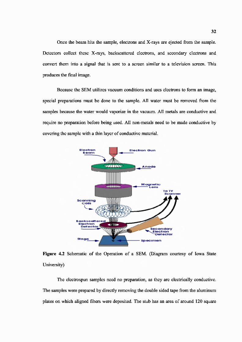
The SEM is an instrument that produces a largely magnified image by using
electrons instead of light to form an image. A beam of electrons is produced at the top of
the microscope by an electron gun. The electron beam follows a vertical path through the
microscope, which is held within a vacuum. The beam travels through electromagnetic
fields and lenses, which focus the beam down toward the sample (Figure 4.2).
32
Once the beam hits the sample, electrons and X-rays are ejected from the sample.
Detectors collect these X-rays, backscattered electrons, and secondary electrons and
convert them into a signal that is sent to a screen similar to a television screen. This
produces the final image.
Because the SEM utilizes vacuum conditions and uses electrons to form an image,
special preparations must be done to the sample. All water must be removed from the
samples because the water would vaporize in the vacuum. All metals are conductive and
require no preparation before being used. All non-metals need to be made conductive by
covering the sample with a thin layer of conductive material.
Figure 4.2 Schematic of the Operation of a SEM. (Diagram courtesy of Iowa State
University)
The electrospun samples need no preparation, as they are electrically conductive.
The samples were prepared by directly removing the double sided tape from the aluminum
plates on which aligned fibers were deposited. The stub has an area of around 120 square
33
millimeters, so the specimen samples were stuck in such a way that 4 to 5 could fit into the
stub. A layer of carbon tape (double sided) is pasted to the stubs and the sample is stuck to
the other side of the tape. Carbon tapes are used to prevent the charging of the sample.
Carbon tapes dissipate the excessive charge buildup. The specimen fixed stubs was then
mounted on the microscope chamber. To begin with the image capturing, proper spot size
and accelerating voltage should be selected. Higher accelerating voltage will increase
resolution, but also increases specimen damage, contamination, and charging, and
decreases surface detail.
Therefore, a voltage of 1 kV was used for all the samples. After setting the voltage,
the samples were magnified to the desired size. The processes of stigmation, apertures
align and focus was repeated for proper black level and gain level for clarity and was
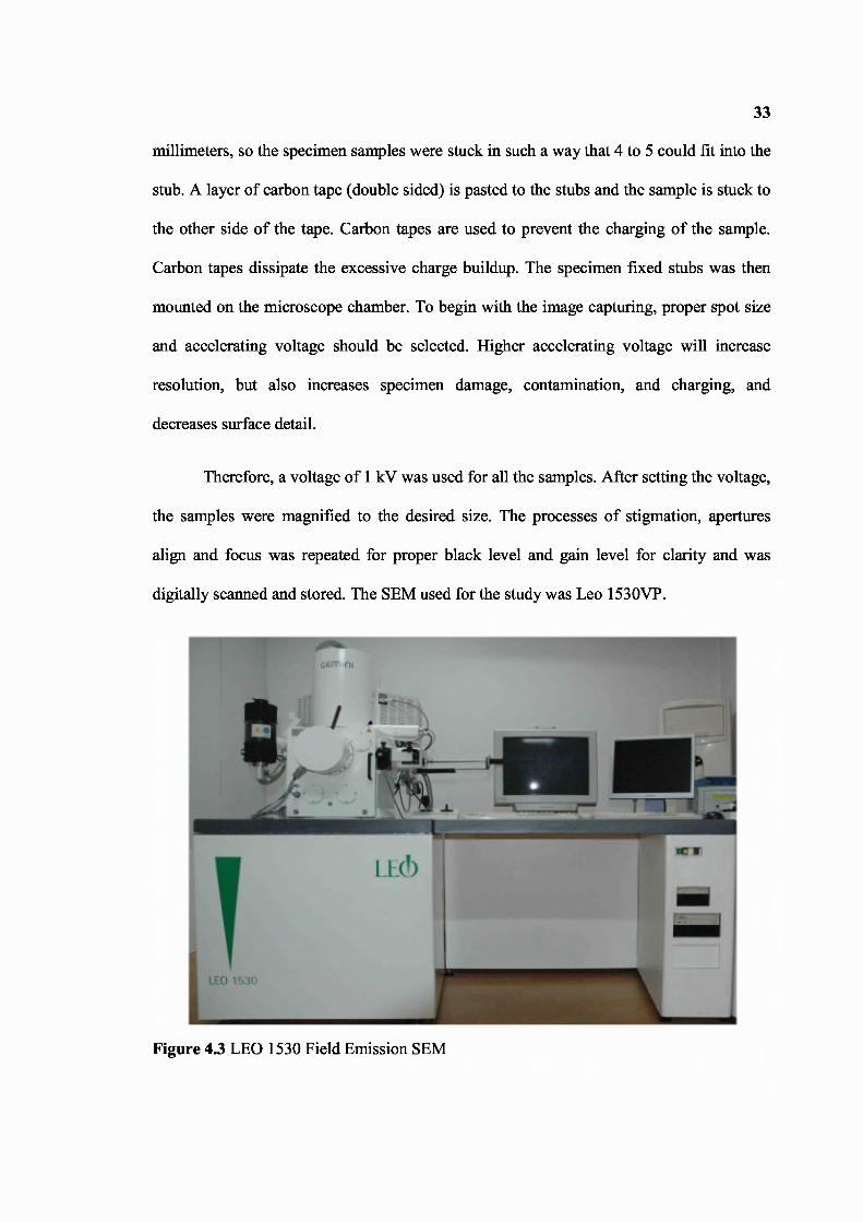
digitally scanned and stored. The SEM used for the study was Leo 1530VP.
Figure 4.3 LEO 1530 Field Emission SEM
34
The analyses of the electrospun nanofibers were done with the help of LEO 1530
Field Emission SEM (Figure 4.3). The LEO 1530 is an ultra-high resolution field emission
SEM utilizing the GEMINI field emission column. It is well suited to a wide range of
applications due to its versatile specimen chamber and eucentric stage. Six free ports for
the attachment of optional detectors and accessories enable the instrument to be used as a
complete analytical workstation.
The electrospun nanofibers samples used in this method were coated. The SEM
was interfaced with computer having LEO 320 software. Since the scanning electron
microscope uses a high voltage for its operation and the electron beam is so sharp and
intense that a small speck of dust in the system or in the sample may ruin the measurement
of the whole sample. So proper care must be taken while preparing the sample and
mounting the sample on the microscope.
4.5 Mechanical Properties
The atomic force microscope (AFM) can image the three-dimensional structure of
nanofibers in a physiological environment enabling real-time biochemical and
physiological processes to be monitored at a resolution similar to that obtained for the
electron microscope (EM). The process of image acquisition with the AFM probe allows
forces to be measured at the molecular level [61]. Indentation of Nano-materials with the
AFM tip provides detailed micromechanical properties. The indentation method existed
prior to the development of the AFM and is a convenient test to assess the mechanical
properties.

35
4.5.1 AFM Development & Principle of Operation
The atomic force microscope (AFM) or scanning force microscope (SFM) was
invented in 1986 by Binnig, Quate and Gerber [62]. Similar to other scanning probe
microscopes, the AFM raster scans a sharp probe over the surface of a sample and
measures the changes in force between the probe tip and the sample. Figure 4.4 illustrates
the working concept for an atomic force microscope. A cantilever with a sharp tip is
positioned above a surface. Depending on this separation distance, long range or short
range forces will dominate the interaction. This force is measured by the bending of the
cantilever by an optical lever technique: a laser beam is focused on the back of a cantilever
and reflected into a photodetector. Small forces between the tip and sample will cause less
deflection than large forces. By raster-scanning the tip across the surface and recording the
change in force as a function of position, a map of surface topography and other properties
can be generated [63, 64, 65].
Figure 4.4 Scheme of an atomic force microscope and the force-distance curvecharacteristic of the interaction between the tip and sample [62].
The AFM is useful for obtaining three-dimensional topographic information of
insulating and conducting structures with lateral resolution down to 1.5 nm and vertical
resolution down to 0.05 nm. These samples include clusters of atoms and molecules,
individual macromolecules, and biologic al species (cells, DNA, proteins). Unlike the
36
preparation of samples for STM imaging, there is minimal sample preparation involved for
AFM imaging. Similar to STM operation, the AFM can operate in gas, ambient, and fluid
environments and can measure physical properties including elasticity, adhesion, hardness,
friction and chemical functionality [63, 64, 65].
Basic set-up of an AFM
In principle the AFM resembles a record player and a stylus profilometer. The ability of
an AFM to achieve near atomic scale resolution depends on the three essential
components: (1) a cantilever with a sharp tip, (2) a scanner that controls the x -y-z position,
and (3) the feedback control and loop.
1. Cantilever with a sharp tip . The stiffness of the cantilever needs to be less theeffective spring constant holding atoms together, which is on the order of 1 - 10nN/nm. The tip should have a radius of curvature less than 20-50 nm (smaller isbetter) a cone angle between 10-20 degrees.
2. Scanner. The movement of the tip or sample in the x, y, and z-directions iscontrolled by a piezo-electric tube scanner, similar to those used in STM. Fortypical AFM scanners, the maximum ranges are 80 µm x 80 µm in the x -y planeand 5 µm for the z-direction.
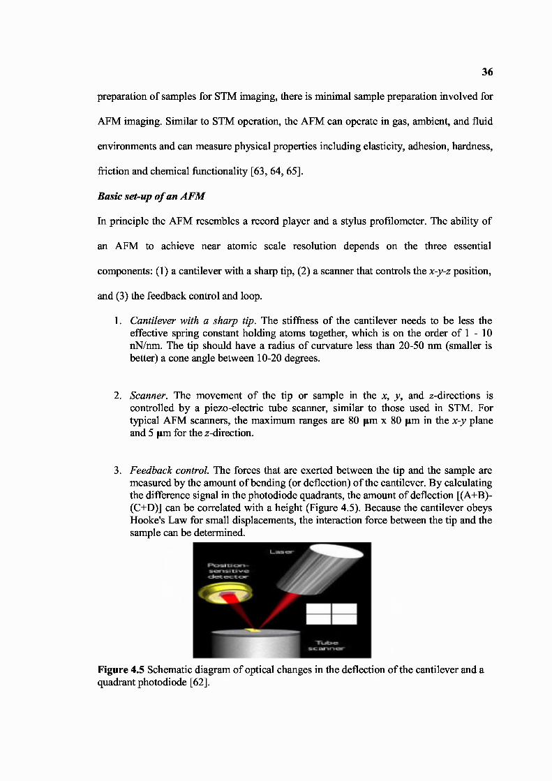
3. Feedback control. The forces that are exerted between the tip and the sample aremeasured by the amount of bending (or deflection) of the cantilever. By calculatingthe difference signal in the photodiode quadrants, the amount of deflection [(A+B)-(C+D)] can be correlated with a height (Figure 4.5). Because the cantilever obeysHooke's Law for small displacements, the interaction force between the tip and thesample can be determined.
Figure 4.5 Schematic diagram of optical changes in the deflection of the cantilever and aquadrant photodiode [62].

37
The AFM can be operated with or without feedback control. If the electronic
feedback is on, as the tip is raster-scanned across the surface, the piezo will adjust the tip-
sample separation so that a constant deflection is maintained—or so the force is the same
as its setpoint value. This operation is known as constant force mode , and usually results in
a fairly faithful topographical (hence the alternative name, height mode).
If the feedback electronics are switched off, then the microscope is said to be
operating in constant height or deflection mode. This is particularly useful for imaging
very flat samples at high resolution. Strictly, this mode should then be called error signal .
The error signal may also be displayed while the feedback is on; this image displays slow
variations in topography and highlights the edges of features [63, 64].
4.5.2 Modes of operation for the AFM
The three general types of AFM imaging are contact mode, tapping mode and non-contact
mode [63, 64].
Contact mode
Contact mode is the most common method of operation of the AFM and is useful for
obtaining 3D topographical information on nanostructures and surfaces. “Contact”
represents the repulsive regime of the inter- molecular force curve, the part of the curve
above the x-axis (Figure 4.6, right image). Most cantilevers have spring constants < 1 Nm,
which is less than effective spring constant holding atoms together.
Figure 4.6 Scheme of contact mode imaging and an image of cholera oligomers [63].
38
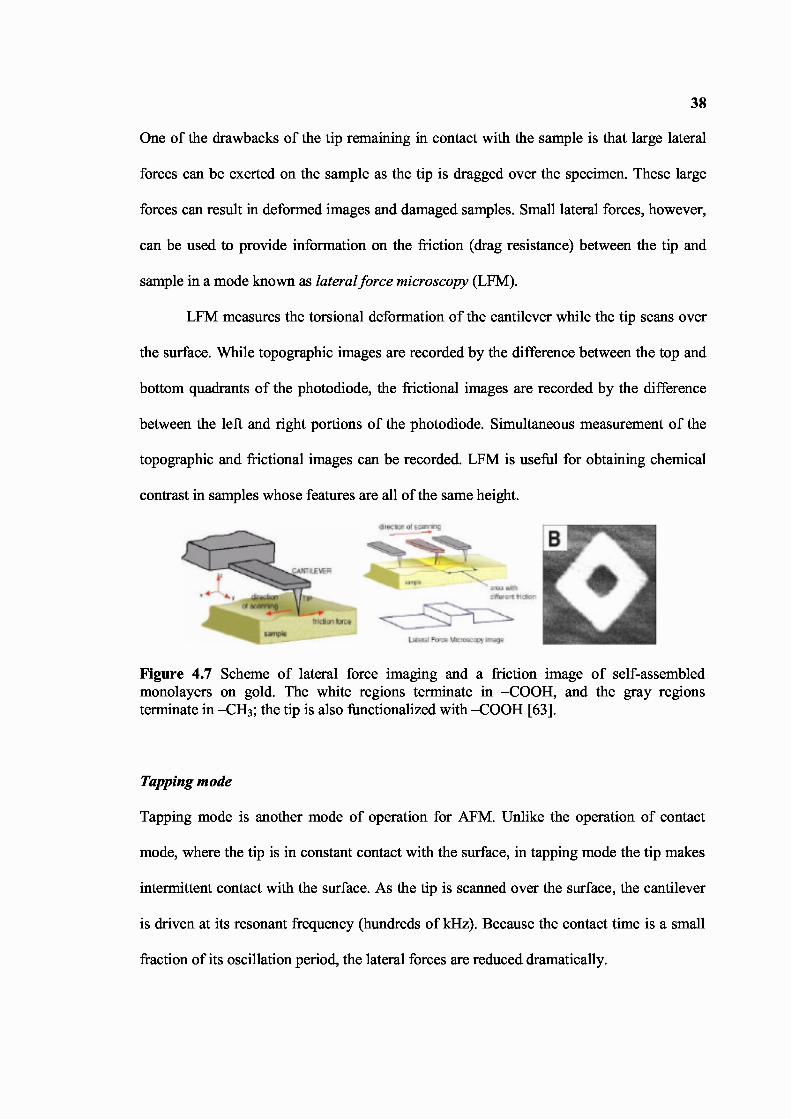
One of the drawbacks of the tip remaining in contact with the sample is that large lateral
forces can be exerted on the sample as the tip is dragged over the specimen. These large
forces can result in deformed images and damaged samples. Small lateral forces, however,
can be used to provide information on the friction (drag resistance) between the tip and
sample in a mode known as lateral force microscopy (LFM).
LFM measures the torsional deformation of the cantilever while the tip scans over
the surface. While topographic images are recorded by the difference between the top and
bottom quadrants of the photodiode, the frictional images are recorded by the difference
between the left and right portions of the photodiode. Simultaneous measurement of the
topographic and frictional images can be recorded. LFM is useful for obtaining chemical
contrast in samples whose features are all of the same height.
Figure 4.7 Scheme of lateral force imaging and a friction image of self-assembledmonolayers on gold. The white regions terminate in –0OOH, and the gray regionsterminate in –0H 3 ; the tip is also functionalized with –0OOH [63].
Tapping mode
Tapping mode is another mode of operation for AFM. Unlike the operation of contact
mode, where the tip is in constant contact with the surface, in tapping mode the tip makes
intermittent contact with the surface. As the tip is scanned over the surface, the cantilever
is driven at its resonant frequency (hundreds of kHz). Because the contact time is a small
fraction of its oscillation period, the lateral forces are reduced dramatically.
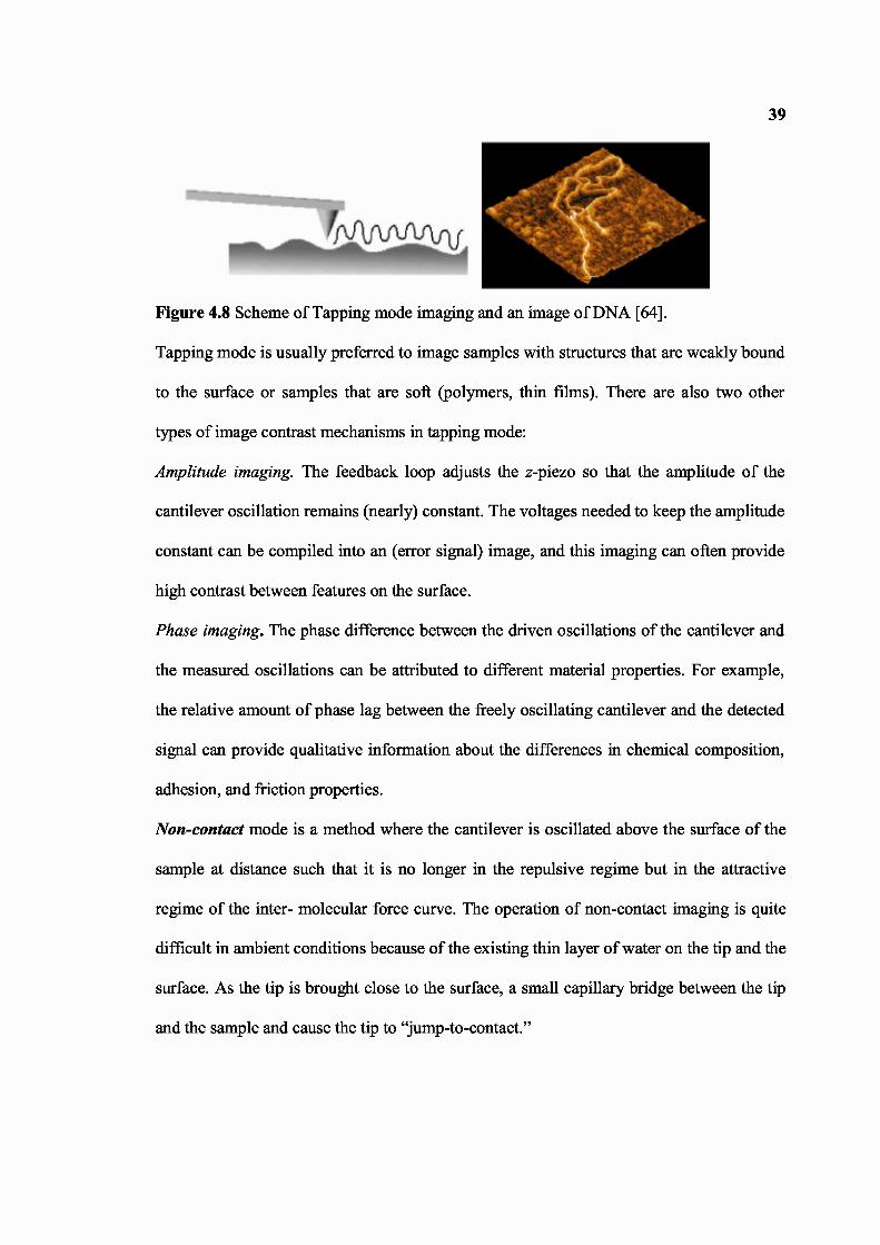
39
Figure 4.8 Scheme of Tapping mode imaging and an image of DNA [64].
Tapping mode is usually preferred to image samples with structures that are weakly bound
to the surface or samples that are soft (polymers, thin films). There are also two other
types of image contrast mechanisms in tapping mode:
Amplitude imaging. The feedback loop adjusts the z-piezo so that the amplitude of the
cantilever oscillation remains (nearly) constant. The voltages needed to keep the amplitude
constant can be compiled into an (error signal) image, and this imaging can often provide
high contrast between features on the surface.
Phase imaging . The phase difference between the driven oscillations of the cantilever and
the measured oscillations can be attributed to different material properties. For example,
the relative amount of phase lag between the freely oscillating cantilever and the detected
signal can provide qualitative information about the differences in chemical composition,
adhesion, and friction properties.
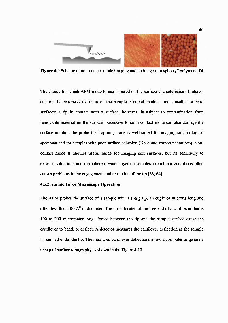
Non-contact mode is a method where the cantilever is oscillated above the surface of the
sample at distance such that it is no longer in the repulsive regime but in the attractive
regime of the inter- molecular force curve. The operation of non-contact imaging is quite
difficult in ambient conditions because of the existing thin layer of water on the tip and the
surface. As the tip is brought close to the surface, a small capillary bridge between the tip
and the sample and cause the tip to “jump-to-contact.”
40
Figure 4.9 Scheme of non-contact mode imaging and an image of raspberry” polymers, DI
The choice for which AFM mode to use is based on the surface characteristics of interest
and on the hardness/stickiness of the sample. Contact mode is most useful for hard
surfaces; a tip in contact with a surface, however, is subject to contamination from
removable material on the surface. Excessive force in contact mode can also damage the
surface or blunt the probe tip. Tapping mode is well-suited for imaging soft biological
specimen and for samples with poor surface adhesion (DNA and carbon nanotubes). Non-
contact mode is another useful mode for imaging soft surfaces, but its sensitivity to
external vibrations and the inherent water layer on samples in ambient conditions often
causes problems in the engagement and retraction of the tip [63, 64].
4.5.2 Atomic Force Microscope Operation
The AFM probes the surface of a sample with a sharp tip, a couple of microns long and
often less than 100 A0 in diameter. The tip is located at the free end of a cantilever that is
100 to 200 micrometer long. Forces between the tip and the sample surface cause the
cantilever to bend, or deflect. A detector measures the cantilever deflection as the sample
is scanned under the tip. The measured cantilever deflections allow a computer to generate
a map of surface topography as shown in the Figure 4.10.
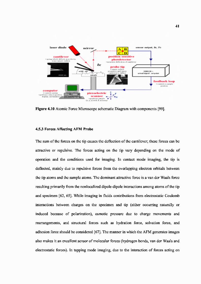
41
Figure 4.10 Atomic Force Microscope schematic Diagram with components [99].
4.5.3 Forces Affecting AFM Probe
The sum of the forces on the tip causes the deflection of the cantilever; these forces can be
attractive or repulsive. The forces acting on the tip vary depending on the mode of
operation and the conditions used for imaging. In contact mode imaging, the tip is
deflected, mainly due to repulsive forces from the overlapping electron orbitals between
the tip atoms and the sample atoms. The dominant attractive force is a van der Waals force
resulting primarily from the nonlocalized dipole-dipole interactions among atoms of the tip
and specimen [62, 65]. While imaging in fluids contributions from electrostatic Coulomb
interactions between charges on the specimen and tip (either occurring naturally or
induced because of polarization), osmotic pressure due to charge movements and
rearrangements, and structural forces such as hydration force, solvation force, and
adhesion force should be considered [67]. The manner in which the AFM generates images
also makes it an excellent sensor of molecular forces (hydrogen bonds, van der Waals and
electrostatic forces). In tapping mode imaging, due to the interaction of forces acting on
42
the cantilever when the tip comes close to the surface, Van der Waals force, dipole-dipole
interaction, electrostatic forces, etc. cause the amplitude of this oscillation to decrease as
the tip gets closer to the sample. An electronic servo uses the piezoelectric actuator to
control the height of the cantilever above the sample. The servo adjusts the height to
maintain a set cantilever oscillation amplitude as the cantilever is scanned over the sample.
A tapping AFM image is therefore produced by imaging the force of the intermittent
contacts of the tip with the sample surface [68, 69].
4.5.4 Measuring the Elastic Properties with the AFM
Other methods have been used to measure the elastic properties are flicker spectroscopy
[70], and optical tweezers [71, 72]. Bereiter-Hahn and coworkers used another scanning
microscopy technique, scanning acoustic microscopy, to measure the elastic properties of
cells locally [73, 74]. The main difference between AFM and these techniques is the high
lateral resolution (100 nm) provided by the AFM with the potential to increase with
improved tip design [75].
AFM data can be interpreted as elasticity measurements [76-79]. The AFM allows
the mechanical properties of fibers to be determined accurately from force-versus-distance
curves (force curves) [80, 81]. The relationship between indentation force and depth
depends upon the tip geometry and the mechanical properties of the specimen [82].
If the sample is soft, the tip will deform it, and elastic indentation occurs. The force
versus indentation curves becomes non-linear for softer samples, because the compliance
of the sample becomes higher for larger loading forces. Radmacher considers the geometry
of AFM tips to be conical, on a scale of several 10's to 100s of nm [75]. The contact area
of the probe increases with indentation, the force-depth relationship in any soft material is
43
nonlinear, making it difficult to assess how much of the response is due to the tip geometry
[82]. Since, the contact area will increase while loading, indenting the sample. This
process has been treated analytically by Hertz, where a relationship between the
indentation and the loading force is given for smooth parabolic indenter profiles [83]. Most
investigators have attributed nonlinearity of the indentation response entirely to the tip
geometry, and have applied equations based on classical infinitesimal strain theory to
extract the Young's modulus (E) of the material [84, 85].
4.5.5 Assumptions and Challenges
There are many assumptions that must hold for an accurate modulus determination with
the Hertz model, including that the material is linear elastic, homogeneous, and in finitely
thick, with no adhesion or attraction between the tip and the sample. Care must be taken to
ensure that the sample in question can be described within these assumptions or that the
deviations from these assumptions are considered. Although most biological materials
have viscoelastic properties, at the indentation rates (2 μm/s) and depths (<100 nm)
typically used in AFM nanoindentation, the force curves can be consistent with a linear
elastic material and an elastic modulus can be de fined. If the force curves show any
indication of viscoelasticity (hysteresis in the loading and unloading curves in the force
curve) or sample adhesion, it may not be appropriate to use the Hertz model or to define an
elastic modulus. The range of indentation depths that can be accurately modeled is also
dependent on the sample thickness. For soft or thin samples (and larger indentation
depths), the influence of the substrate on the measured elastic modulus must be considered.
The elastic modulus can be plotted as a function of indentation depth, and it can be veri fied
that the elastic modulus is independent of indentation depth for at least small indentation
depths. An increase in modulus with indentation depth may be indicative of an increasing
44
contribution from the substrate. It is also important to note that the AFM measures the
modulus at the surface of the material and may be more accurately termed local modulus.
Measuring a local modulus can be advantageous for certain experiments. For example, this
allows a determination of the substrate elastic modulus a cell would sense on the surface of
the substrate. Additionally, any heterogeneity in modulus across the substrate can be
observed by obtaining a force map. It should also be noted that with the AFM, the modulus
is measured in compression as the AFM tip is indented into the sample surface. The
modulus measured with AFM may, therefore, be different from that obtained from other
techniques, such as tensile testing, because of the differences in the direction of applied
strain and any anisotropy of the sample. In addition, tensile testing measures the modulus
of the sample in its entirety, whereas the AFM will be sensitive to changes in the
mechanical properties between the surface and the bulk.
The Hertz equation also requires accurate knowledge of the initial contact point of
the tip with the sample. This value can be difficult to determine from the force curves,
particularly when there is tip-sample attraction or there is water or a contamination layer
on the sample surface that the tip senses before it comes in contact with the surface. The
Hertz equation can be fitted to the experimental data with two unknowns in the equation,
fitting for both E and Zo, the initial contact point. This eliminates the need to choose the
value of Zo manually. The user must still be aware that changes in the value of Zo can
significantly affect the calculated modulus value.
Accurate determination of the elastic modulus requires accurate calibration of the
system, including the scanner and the cantilever. Calibration of the scanner must be
checked periodically with an appropriate calibration grid for the size of the scanner. Each
cantilever must also be calibrated so that the de flection sensitivity and the spring constant
45
are known. The deflection sensitivity (nm/V) is found by taking a force curve on a hard
surface, with no indentation into the surface. In this case d = z, and the sensitivity is the
slope of the deflection (d) versus z force curve. The deflection sensitivity must be
calculated each time the laser is realigned on the cantilever. The spring constant must also
be determined for each cantilever because the actual value may vary signi ficantly from the
nominal value provided by the manufacturer. There are several techniques that have been
used to measure spring constants [86-96].
The advantages and disadvantages of each available method have been reviewed
by Clifford and Seah [97]. Two popular methods are the Sader method, an equation that
relates the spring constant to the length and width of the cantilever and the cantilever’s
resonant frequency, and the thermal tune method, which measures the cantilever’s
response to thermal noise. [91, 93-95]. In some instruments, the thermal tune method has
been incorporated into the instrument hardware and software.
4.5.6 Tip and Cantilever Selection and Tip Functionalization
Proper choice of both cantilever stiffness and geometry of the incorporated tip are
necessary for successful application of the AFM. Commercially available cantilevers have
spring constants ranging from 0.006 N/m to 200 N/m. The spring constant used in our case
was 0.041nN/nm, which was given by the manufacturer Brukers AFM. To avoid surface
damage of nanofiber samples, imaging in contact mode and tapping mode, in either air or
fluid, requires cantilevers with low spring constants, typically < 0.2 N/m. As mentioned
previously, tapping mode is more generally used when imaging soft, biological samples. A
low spring constant cantilever is also used for tapping mode in fluid, whereas a stiffer
cantilever (typically approximately 45 N/m) is needed for tapping mode in air to reduce

46
noise. Low spring constant cantilevers also provide better de flection resolution, with a
larger deflection for a given force, necessary for measuring intermolecular interactions,
which typically range from 10 -12 N to 10 -7 N. The tip can be functionalized with molecules,
proteins, or cells and the interactions of these tips with a surface of interest can be
obtained. Several reviews are available describing these types of experiments [98].
AFM cantilevers with varying tip shapes are available. The standard geometry is of
an integrated pyramidal tip with an end radius of 20 to 30 nm; sharper tips are also
available. Radius of the tip for our probe was 15 nm, which was given by the manufacturer
Brukers AFM. Sharper tips have the advantage of producing images with higher
resolution. Sharper tips, however, have been shown to quickly deteriorate during scanning
of cells, most likely because of tip contamination and blunting. Additionally, sharper tips
have been associated with inducing increased damage to the cell surface.
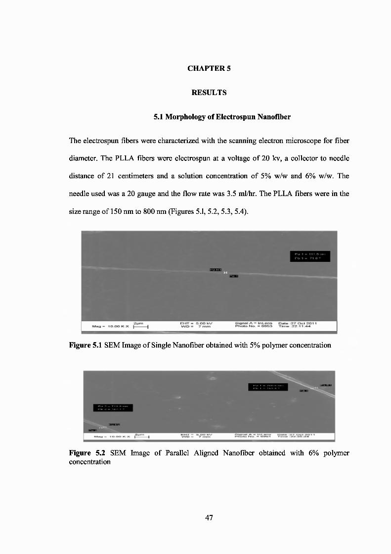
CHAPTER 5
RESULTS
5.1 Morphology of Electrospun Nanofiber
The electrospun fibers were characterized with the scanning electron microscope for fiber
diameter. The PLLA fibers were electrospun at a voltage of 20 kv, a collector to needle
distance of 21 centimeters and a solution concentration of 5% w/w and 6% w/w. The
needle used was a 20 gauge and the flow rate was 3.5 ml/hr. The PLLA fibers were in the
size range of 150 nm to 800 nm (Figures 5.l, 5.2, 5.3, 5.4).
Figure 5.1 SEM Image of Single Nanofiber obtained with 5% polymer concentration
Figure 5.2 SEM Image of Parallel Aligned Nanofiber obtained with 6% polymerconcentration
47
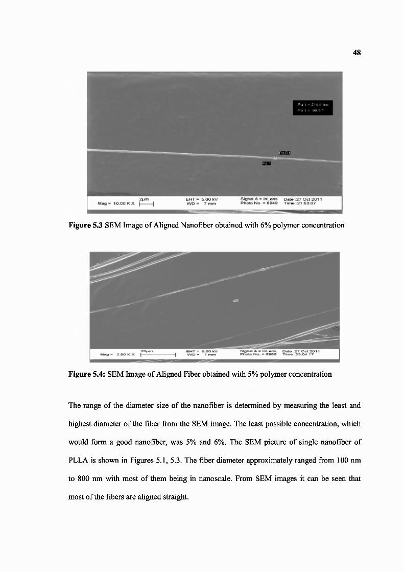
48
Figure 5.3 SEM Image of Aligned Nanofiber obtained with 6% polymer concentration
Figure 5.4: SEM Image of Aligned Fiber obtained with 5% polymer concentration
The range of the diameter size of the nanofiber is determined by measuring the least and
highest diameter of the fiber from the SEM image. The least possible concentration, which
would form a good nanofiber, was 5% and 6%. The SEM picture of single nanofiber of
PLLA is shown in Figures 5.1, 5.3. The fiber diameter approximately ranged from 100 nm
to 800 nm with most of them being in nanoscale. From SEM images it can be seen that
most of the fibers are aligned straight.

49
Polymer Concentration Vs FiberDiameter
PLLA Polymer Concentration (W/W%)
400
300
700
600
500
200
100
0
5%
6%
Figure 5.5: Bar Graph Representation of Polymer Concentration Vs Fiber Diameter.
The fiber diameter was obtained in nanoscale dimensions, by using the polymer
concentration with 5% w/w, 6% w/w. The graph shows the standard deviation valves for
both the concentration were in the 184.3 nm and 230.2 nm respectively and mean valve of
both the concentration were 364.9 nm and 418.1 nm.
5.2 Mechanical Characterization of Electrospun Nanofibers
The AFM image of single nanofiber of PLLA is shown in Figures 5.6, 5.7. The left side
image is tapping mode image where, the height of the nanofiber is visible. The right side
image is phase image which is obtained with tapping mode image and phase shift signal is
visible from the image. The brightness in the image shows, the amplitude is less and tip is
in close contact with the sample. The contrast in the image shows, the amplitude is more

50
and is not in contact with the sample. This difference is because, the surface is rough and
result which this image gives is the tip scan over the surface and based on the roughness of
the surface, amplitude is changing with constant force maintained by feedback signal
operating through computer software.
Figure 5.6: AFM Image of Parallel Aligned Nanofiber obtained with 5% polymerconcentration
Figure 5.7: AFM Image of Single Nanofiber obtained with 5% polymer concentration
The image of nanofiber diameter obtained in tapping mode AFM is in range of 167 nm.
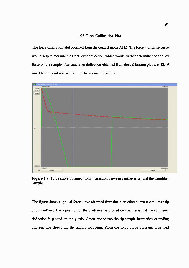
51
5.3 Force Calibration Plot
The force calibration plot obtained from the contact mode AFM. The force – distance curve
would help to measure the Cantilever deflection, which would further determine the applied
force on the sample. The cantilever deflection obtained from the calibration plot was 12.19
nm. The set point was set to 0 mV for accurate readings.
Figure 5.8: Force curve obtained from interaction between cantilever tip and the nanofibersample.
The figure shows a typical force curve obtained from the interaction between cantilever tip
and nanofiber. The z position of the cantilever is plotted on the x-axis and the cantilever
deflection is plotted on the y-axis. Green line shows the tip sample interaction extending
and red line shows the tip sample retracting. From the force curve diagram, it is well
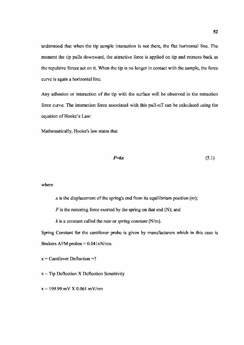
52
understood that when the tip sample interaction is not there, the flat horizontal line. The
moment the tip pulls downward, the attractive force is applied on tip and retraces back as
the repulsive forces act on it. When the tip is no longer in contact with the sample, the force
curve is again a horizontal line.
Any adhesion or interaction of the tip with the surface will be observed in the retraction
force curve. The interaction force associated with this pull-off can be calculated using the
equation of Hooke’s Law:
Mathematically, Hooke's law states that
F=kx (5.1)
where
x is the displacement of the spring's end from its equilibrium position (m);
F is the restoring force exerted by the spring on that end (N); and
k is a constant called the rate or spring constant (N/m).
Spring Constant for the cantilever probe is given by manufacturers which in this case is
Brukers AFM probes = 0.041nN/nm.
x = Cantilever Deflection =?
x = Tip Deflection X Deflection Sensitivity
x = 199.99 mV X 0.061 mV/nm
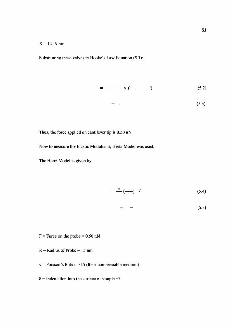
53
X = 12.19 nm
Substituting these valves in Hooke’s Law Equation (5.1):
. x ( . ) (5.2)
. (5.3)
Thus, the force applied on cantilever tip is 0.50 nN
Now to measure the Elastic Modulus E, Hertz Model was used.
The Hertz Model is given by
V ( ) / (5.4)
=
F = Force on the probe = 0.50 nN
R = Radius of Probe = 15 nm.
v = Poisson’s Ratio = 0.5 (for incompressible medium)
(5.5)
8 = Indentation into the surface of sample =?
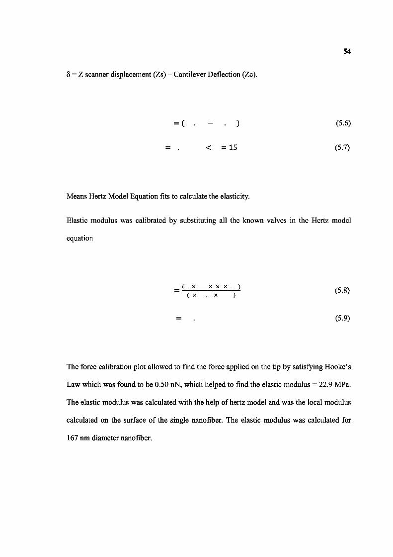
54
8 = Z scanner displacement (Zs) – Cantilever Deflection (Zc).
= ( — ) (5.6)
< = 15 (5.7)
Means Hertz Model Equation fits to calculate the elasticity.
Elastic modulus was calibrated by substituting all the known valves in the Hertz model
equation
( x x x x ) = ( ) (5 . 8)x x
(5.9)
The force calibration plot allowed to find the force applied on the tip by satisfying Hooke’s
Law which was found to be 0.50 nN, which helped to find the elastic modulus = 22.9 MPa.
The elastic modulus was calculated with the help of hertz model and was the local modulus
calculated on the surface of the single nanofiber. The elastic modulus was calculated for
167 nm diameter nanofiber.
CHAPTER 6
DISCUSSION
The results show that the aligned nanofiber is the best way to study the characterization of
single nanofiber, as it is easy to mount on stub of characterization technique to know about
its morphology and mechanical properties. Here a unique approach was developed and
used to handle and isolate the nanofiber by sticking double sided tape on aluminum plates
arranged in parallel employed on electrospinning technique, which made possible to study
the morphological and mechanical properties with ease as sample was properly mounted
on stub. The alignment and fiber diameter in nanoscale dimensions was confirmed with the
images obtained in Scanning Electron Microscope (SEM).
Atomic Force Microscope (AFM) was used to obtain the 3 dimensional image of
nanofiber. Although AFM is not widely used in PLLA nanofiber research, many questions
in polymer science can be addressed by use of this technique. The ability of the AFM to
provide high-resolution images and to sense small forces in the sample’s native
environment make this technique invaluable in the characterization of nanofibers.
Currently, the AFM has been used to determine the function of nanofiber made of PLLA
with high-resolution imaging, to explore and quantify tip sample interactions, to
characterize how nanoscale topography acts, to determine the mechanical properties of
nanofiber in their native environment, and to help understand how a change in fiber
diameter correlates with mechanical properties. The AFM can be used alone or can be
combined with other optical and spectroscopic techniques to provide complementary
information, creating an even more powerful tool. Also the person performing the
55
experimentation should be expert in handling AFM. Proper training is required to get the
accurate results. The sharper you are in using AFM, the more well will be your results.
Proper care should be care will mounting sample on AFM to avoid dust particles to settle
down on stub. To have good judgment about the nanofiber in AFM, vast knowledge of
AFM is necessary with at least 2 months of practice.
Calibration of force curve plot was done in Stevens Institute of Technology, as the
software of multimode AFM in New Jersey Institute of Technology was not updated. The
new version of software is required to obtain the results. The version currently used in
New Jersey Institute of Technology is 4.4 3r5. As per the talk with technical support team
of Brukers AFM Company, the new version can provide very good results with respect to
both imaging and force calibration. The application of AFM will benefit evolving various
other properties of nanofiber with application to polymer science. In this study, AFM was
used to for measuring the force applied on the tip and also the elastic modulus of a
nanofiber.
56

CHAPTER 7
CONCLUSIONS
The process of electrospinning was successfully carried out using PLLA as the polymer
and methylene chloride as the solvent. By varying the concentration and the needle
diameter, the process of electrospinning yielded very fine fibers with diameters in the
nanometer range as well as fibers in the micron range. The nanofibers were selected for
characterizing the mechanical properties using Scanning Electron Microscope and Atomic
Force Microscope.
The electrospun nanofibers were cylindrical of varying diameters. The results of
the SEM characterization showed that through electrospinning process, using PLLA 5%
dissolving in methylene chloride as a solvent and maintaining flow rate of 3.5ml/hr, at 20
kV voltage, nanofibers in the range of 100 nm to 800 nm were obtained. The electrospun
fibers had a good alignment with the help of parallel arrangement method used in
electrospinning technique, which was favorable for mounting the sample for mechanical
testing.
The AFM enabled us to image the three-dimensional structure of nanofiber
allowing us to monitor its morphology and mechanical property. The tapping mode
imaging and phase imaging was obtained and its morphological characteristic was
observed. The force applied during the scanning was determined by using contact mode
AFM, satisfying Hooke’s Law, and was found to be 0.50 nN. To determine the mechanical
properties of nanofiber, elasticity was measured with the help of Hertz Model and was
obtained upto 22.9 MPa.
57

CHAPTER 8
FUTURE SCOPE OF RESEARCH
i. A study needs to be conducted to investigate how the diameter and distribution of
diameter is affecting the mechanical properties of the aligned nanofiber.
ii. To obtain aligned nanofiber of different materials/polymer.
iii. Measure characterization and mechanical properties of different materials/polymer.
iv. Measure various other mechanical properties like tensile properties on single
aligned nanofiber by innovating the mounting technique to measure it.
v. Future experiments should involve more analysis of nanofibers mechanical testing.
This could be accomplished by analyzing data from indentations occurring at
different rates.
vi. Measure the Elastic Modulus of different diameter nanofiber and compare.
58
REFERENCES
1. Fibers, [Document posted on the Website of Department of polymer Science,University of Southern Mississippi] Retrieved on December 2003 from the WorldWide Web. http://www.psrc.usm.edu/macrog/fiber.html . Accessed 10/03/2011
2. J. M. Deitzel, J. Kleinmeyer, D. Harris and N. C. Beck Tan (2001). The effect ofprocessing variables on the morphology of electrospun nanofibers and textiles.Polymer, Volume 42(1), 261-272
3. Formhals A, Process and apparatus for preparing artificial threads. US Patent(1934),l,975,504.
4. Baumgarten PK. (1971) Electrostatic Spinning of Acrylic Microfibers. Journal ofColloid and Interface Science, Vol. 36(1), 71-79
5. Larrondo I, Manley RS. (1981) Journal of Polymer Science: Polymer PhysicsEdition, 19, 909-20
6. Zheng-Ming Huang, Y.Z. Zhang, M. Kotaki, S. Ramakrishna(2003). A review onpolymer nanofibers by electrospinning and their applications in nanocomposites;Composites Science and Technology 63, 2223-2253.
7. E.P.S. Tan, C.T. Lim. Mechanical characterization of nanofibers – A reviewComposites Science and Technology 66 (2006) 1102–1111.
8. Rayleigh, F. R. S., Phil., Mag. (1882) 44, p.184. Accessed 10/07/2011
9. Zeleny, J., Physical Review, (1914) 3, p. 69. Accessed 10/07/2011
10.Vonnegut, B., and Neubauer, R.I., Journal of Colloid Science (1952) 7, p. 616.Accessed 10/07/2011
11. Watchel, R.E., and Iamer, V.K., Journal of Colloid Science (1962) 17, p. 531.Accessed 10/08/2011
59
60
12. Taylor GI. Electrically Driven Jets. Proceedings of the Royal Society of LondonSeries (1969) A Mathematical and Physical Sciences. Vol. 313, 453-475
13. Gladding, E.K., U.S Patent,(1939) 2,168,027. Accessed 10/15/2011
14. Simons H.I., U.S Patent,(1966) 3,280,229. Accessed 10/15/2011
15.Bomat A., U.S Patent, (1982) 4,323,525. Accessed 10/15/2011
16.Baumgarten PK (1971). Electrostatic Spinning of Acrylic Microfibers; Journal ofColloid and Interface Science, Vol. 36(1), 71-79
17. Larrondo, I., and Manley, R.ST.J. (1981) Journal of polymer physics Edition,Volume 63 p.909.
18.Kim J-S, Reneker DH. (1999) Mechanical Properties of Composites UsingUltrafine Electrospun Fibers. Polymer Science, 39(5) p. 849-854.
19.Doshi J, Reneker DH.(1995). Electrospinning Process and Applications ofElectrospun Fibers; Journal of Electrostatics,35, 151-160
20. Srinivasan G, Reneker DH. (1995). Structure and Morphology of Small diameterElectrospun Aramid fibers; Polymer intemationa1, 36,195-201
21. Reneker DH, Chun I.(1996) Nanometer diameter fibers of polymer, produced byElectrospinning; Nanotechnology, 7, 216-223
22. Fang X, Reneker DH.(1997).DNA fibers by electrospinning; Journal ofmacromolecular science: Physics, Volume 36, Pages 1-428
23. Deitzel, J. M.; BeckTan, N. C.; Kleinmeyer, J. D.; Rehrmann, J.; Tevault, D.Army Research Laboratory Technical Report 1999, ARL-TR-1989
24. Yarin, A. L.; Koombhongse, S.; Reneker, D. H. J Applied Physics 2001, 89, 5.
61
25. Deitzel, J. M.; Kleinmeyer, J.; Harris, D.; BeckTan, N. C Polymer 2001, 42, 261
26. Ramkumar, S. S.; Sastri, L. ATA J 2002, Aug/Sep, 49.Warner, S. B.; Buer, A.;Grimler, M.; Ugbolue, S. C.; Rutledge, G. C.; Shin, M. Y. National Textile CenterAnnu Report November 1998, 83
27. Jaeger, R.; Bergshoef, M. M.; Batlle, C. M. I.; Holger, S.; Vancso, G. J.Macromol Symp 1998, 127, 141.
28. http://www.espintechnologies.com/ accessed 11/02/2011
29. http://www.donaldson.com/en/ filtermedia/nanofibers/index.html accessed11/02/2011
30. Gibson, P. W.; Gibson, H. L.; Rivin, D. AIChe J 1999, 45, 190.
31. Moses, M.; Hohman, M. M.; Shin, Y. M.; Rutledge, G. C.; Brenner, M. P. PhysFluids 2001, 13, 2201.
32. Moses, M.; Hohman, M. M.; Shin, Y. M.; Rutledge, G. C.; Brenner, M. P. PhysFluids 2001, 13, 2221.
33. Shin, Y. M.; Hohman, M. M.; Brenner, M. P.; Rutledge, G. C. Polymer 2001, 42,9955.
34. Yarin, A. L.; Koombhongse, S.; Reneker, D. H. J Appl Phys 2001, 89, 301.
35. Shin, Y. M.; Hohman, M. M.; Brenner, M. P.; Rutledge, G. C. Applied PhysicsLetter 2001, 78, 1149.
36. Reneker, D. H.; Yarin, A. L.; Fong, H.; Koombhongse, S. J Applied Physics2000, 87, 4531.
37. Fridrikh, S. V.; Yu, J. H.; Brenner, M. P.; Rutledge, G. C. Physical ReviewLetters, 2003, 90, 144502.
62
38. Megelski, S.; Stephens, J. S.; Chase, D. B.; Rabolt, J. F. Macromolecules 2002,35, 8456.
39. Buchko, C. J.; Chen, L. C.; Yu, S.; Martin, D. C. Polymer 1999, 40, 739.
40. Deitzel, J. M.; Kleinmeyer, J. D.; Hirvonen, J. K.; BeckTan, N. C Polymer 2001,42, 8163.
41. Atala, Mooeny et. al.(1997) Synthetic Biodegradable Polymer Scaffolds. Boston,MA: Birkhauser.
42. W.M. Saltzman, R.P Lanza, R. Langer, J. Vancanti, Editors, Principles of TissueEngineering, (2nd edn.), Academic Press, California (2000), p. 221
43. Zheng-Ming Huang, Y.Z. Zhang, M. Kotaki, S. Ramakrishna (2003). A review onpolymer nanofibers by electrospinning and their applications in nanocomposites;Composites Science and Technology 63, 2223-2253.
44. Matalov-Meytal, Y.; Sheintuch, M. Electrospinning of Nanofibers, AppliedCatalysis A: General 2002, 231, 1.
45. http://www.donaldson.com/en/ filtermedia dated 11/18/2011 .
46. http://www.acell.com dated 11/18/2011.
47. Gibson, H.; Gibson, P. http://www.asc2004.com dated 11/18/2011.
48. Doshi, J.; Mainz, M. H.; Bhat, G. S. Nanofibers Nonwovens, Proceedings of the10th TANDEC Conference 2000, Knoxville, TN.
49. Lee, Y.; Bhat, G. Processing and Fabrication of Advanced Materials for HighTemperature Applications, Ed. T. S. Srivatsan and R. A. Varin; The MaterialsSociety: Warrendale, PA, 2003
63
50. http://techreports.larc.nasa.gov/ltrs/PDF/2003/aiaa/NASA-aiaa-2003–1768.pdfaccessed 10/16/2011
51. K.H. Ieea, H.Y. Kimb, M.S. Khilb, Y.M. Rab, D.R. Leeb(2003).Characterizationof nano-structured PCL nonwoven mats via electrospinning; Polymer 44,1287-1294.
52. Perez-Rigueiro J, Viney C, Llorca J, Elices M. Silkworm silk as an engineeringmaterial. J Applied Polymer Science 1998; 70: 2439–47.
53. Yu MF, Dyer MJ, Skidmore GD, Rohrs HW, Lu XK, Ausman KD, et al. Three-dimensional manipulation of carbon nanotubes under a scanning electronmicroscope. Nanotechnology 1999; 10: 244–52.
54. Available from: http://www.zyvex.com Accessed 10/15/2011
55. Demczyk BG, Wang YM, Cumings J, Hetman M, Han W, Zettl A, et al. Directmechanical measurement of the tensile strength and elastic modulus ofmultiwalled carbon nanotubes. Mater Science Eng A – Structure Mater PropMicrostructure Process 2002;334 (1–2): 173–8.
56. Tan EPS, Lim CT. A novel approach to tensile testing of micro- and nanoscalefibers. Rev Science Instrument 2004; 75(8):2581 –5.
57. Namazu T, Isono Y, Tanaka T. Plastic deformation of nanometric single crystalsilicon wire in AFM bending test at intermediate temperatures. JMicroelectromech Syst 2002; 11(2):125–35.
58. Namazu T, Isono Y. Quasi-static bending test of nano-scale SiO2 wire atintermediate temperatures using AFM-based technique. Sensor Actuator A: Phys2002; 104:78–85.
59. Ma PX, Zhang R. Synthetic nano-scale fibrous extracellular matrix. J BiomedMater Res 1999;46:60–72
60. Cheng Zhu, G. B., and Ning Wang. (2000). "Cell Mechanics: Mechanical

64
Response, Cell Adhesion, and Molecular Deformation." Annual. Revised.Biomedical. Eng., 02, I89- 226.
61. Binnig, G. C. F. Q., and C. Gerber. (1986). "Atomic force microscope." Phys.Rev. Lett., 56, 930-933.
62. R. Wiesendanger, Scanning Probe Microscopy and Spectroscopy,(Cambridge: Cambridge University Press, 1994).
63. R. D. Piner, J. Zhu, F. Xu, S. Hong, and C.A. Mirkin, Science 283, 661 (1999)Accessed 10/24/2011
64. Y. Xia and G.M. Whitesides, American Chemical Society, Langmuir 13 , 2059(1997) Accessed 10/24/2011
65. Goodman, F. O. A. N. G. (1991). "Roles of the attractive and repulsive forces inatomic force microscopy." Physical Rev. B, 43, 4728-4731.
66. Lal, R., and Scott A. John. (I994). "Biological applications of atomic forcemicroscopy." Am. J. Physiol., 266(Cell physiology. 35), C1-C21.
67. Butt, H. J. (1991). "Measuring electrostatic, van der Waals, and hydration forcesin electrolyte solutions with an atomic force microscope." Biophys. J., 60, 1438-1444.
68. Hoh, J. H., J.P. Cleveland, C.B. Prater, J.P. Revel, and P.K. Hansma. (1992)."Quantized adhesion detected with the atomic force microscope." J. Am. Chem.Soc., 114,4917-4918.
69. K Zeman, H. E. a. E. S. (1990). "Bending undulations and elasticity of theerythrocyte membrane organization." Europ. Biophys. J., 18, 203-219.
70. Dziedzic, A. A. a. J. (1989). "Internal cell manipulation using infrared lasertraps." Proc. Natl. Acad. Sci., 86, 7914-7918.
71. K Svoboda, C. S., D Branton and SM Block. (1992). "Conformation and elasticity
65
of the isolated red blood cell membrane skeleton." Biophys. J., 63, 784-793.
72. H Luers, K. H., J Litniewski, J Bereiter-Hahn. (1991). "Acoustic microscopy ofcultured cells. Distribution of forces and cytoskeletal elements." Cell Biophys, 18,279-293.
73. Rugar, J. H. a. D. (1984). "Measurement of cellular elastic properties by acousticmicroscopy." J. Micros., 134, 245-260.
74. Radmacher, M. (1997). "Measuring the elastic properties of biological sampleswith the AFM." IEEE Eng. Med. Biol. Mag., 16,47-57.
75. Pethica, J. B. 0, W.C. (1987). "Tip surface interactions in STM and AFM."Physica Scripta Volume T, Volume T19A, 61-66.
76. Colton, N. B. a. R. J. (1989). "Measuring the nanomechanical properties andsurface forces of materials using an atomic force microscope." Journal of VacuumScience & Technology A (Vacuum, Surfaces, and Films), 7(4), 2906-2913.
77. P. Maivald, H.-J. B., S.A.C. Gould, C,B. Prater, B. Drake, J.A. Gurley, V.B.Elings and P.K. Hansma. (1991). "Using force modulation to image surfaceelasticities with the atomic force microscope." Nanotechnology, 2(2), 103-106.
78. N.J. Tao, S. M. L. a. S. L. (1992). "Measuring the microelastic properties ofbiological material." Biophysical Journal, 63(4),1165-1169.
79. A.L. Weisenhorn, P. K. H., T.R. Albrecht and C.F. Quate. (1989). "Forces inatomic force microscopy in air and water." Appl. Phys. Lett., 54(26), 2651-2653.
80. B. Cappella, P. B., C. Frediani, P. Miccoli and C. Ascoli. (1997). "Force-distancecurves by AFM. A powerful technique for studying surface interactions." IEEEEng. Med. Biol. Mag., 16(2), 58-65.
81. Costa, K. D. a. F. C. Y. (1999). "Analysis of indentation: implications formeasuring mechanical properties with atomic force microscopy." J Biomech Eng,121(5),462-71.
66
82. Hertz, H. (1881). "Uber die beruhrung fester elastischer korper (On the contact ofelastic solids)." J. Reine Angew. Mathematik, 92, 156-157.
83. Radmacher, M., Fritz, M., and Hansma, P.K. (1995). "Imaging soft samples withthe atomic force microscope: Gelatin in water and propanol." Biophys. J., 69,264-270.
84. AL Weisenhorn, M. K., S Kasas, V Gotozos, MR Celio and HJ Butt. (1993),"Deformation and height anomaly of soft surfaces studied with the AFM."Nanotechnology, 4, I06-113
85. Butt HJ, Jaschke M. Calculation of thermal noise in atomic-force microscopy.Nanotechnology. 1995; 6:1–7.
86. Chen BY, Yeh MK, Tai NH. Accuracy of the spring constant of atomic forcemicroscopy cantilevers by finite element method. Anal Chem. 2007; 79:1333 –1338.
87. Clifford CA, Seah MP. The determination of atomic force microscope cantileverspring constants via dimensional methods for nanomechanical analysis.Nanotechnology. 2005; 16:1666 –1680.
88. Green CP, Cleveland JP, Proksch R, Mulvaney P, Sader JE. Normal and torsionalspring constants of atomic force microscope cantilevers. Rev Sci Instrum. 2004;75:1988 –1996.
89. Higgins MJ, Proksch R, Sader JE, et al. Noninvasive determination of opticallever sensitivity in atomic force microscopy. Rev Sci Instrum. 2006; 77.
90. Hutter JL, Bechhoefer J. Calibration of atomic-force microscope tips. Rev SciInstrum. 1993; 64:3342–3342.
91. Neumeister JM, Ducker WA. Lateral, normal, and longitudinal spring constants ofatomic-force microscopy cantilevers. Rev Sci Instrum. 1994; 65:2527–2531.
92. Sader JE. Parallel beam approximation for v-shaped atomic-force microscope
67
cantilevers. Rev Sci Instrum. 1995; 66:4583– 4587.93. Sader JE, Chon JWM, Mulvaney P. Calibration of rectangular atomic force
microscope cantilevers. Rev Sci Instrum. 1999; 70:3967–3969.
94. Senden TJ, Ducker WA. Experimental-determination of spring constants inatomic-force microscopy. Langmuir. 1994; 10:1003–1004.
95. Torii A, Sasaki M, Hane K, Okuma S. A method for determining the springconstant of cantilevers for atomic force microscopy. Measurement ScienceTechnology. 1996; 7:179 –184.
96. Clifford CA, Seah MP. Quantification issues in the identification of nanoscaleregions of homopolymers using modulus measurement via AFM nanoindentation.Appl Surf Sci. 2005; 252:1915–1933.
97. Muller DJ, Helenius J, Alsteens D, Dufrene YF. Force probing surfaces of livingcells to molecular resolution. Nat Chem Biol. 2009; 5:383–390.
98. Noy A, Vezenov DV, Lieber CM. Chemical force microscopy. Annu Rev MaterSci. 1997; 27:381– 421.
99. http://web.mit.edu/cortiz/www/nanomechanics.html Accessed 10/29/2011