copyright warning &...
TRANSCRIPT

Copyright Warning & Restrictions
The copyright law of the United States (Title 17, United States Code) governs the making of photocopies or other
reproductions of copyrighted material.
Under certain conditions specified in the law, libraries and archives are authorized to furnish a photocopy or other
reproduction. One of these specified conditions is that the photocopy or reproduction is not to be “used for any
purpose other than private study, scholarship, or research.” If a, user makes a request for, or later uses, a photocopy or reproduction for purposes in excess of “fair use” that user
may be liable for copyright infringement,
This institution reserves the right to refuse to accept a copying order if, in its judgment, fulfillment of the order
would involve violation of copyright law.
Please Note: The author retains the copyright while the New Jersey Institute of Technology reserves the right to
distribute this thesis or dissertation
Printing note: If you do not wish to print this page, then select “Pages from: first page # to: last page #” on the print dialog screen

The Van Houten library has removed some of the personal information and all signatures from the approval page and biographical sketches of theses and dissertations in order to protect the identity of NJIT graduates and faculty.

ABSTRACT
Title of Thesis : Two and Three-Dimensional
Isoparametric Finite Elements for
Axisymmetric Micropolar Elasticity
FUANG YUAN HUANG : Doctor ofEngineering Science, 1986
Thesis directed by : Dr. Sachio Nakamura
Assistant Professor
Department of Mechanical Engineering
Finite element analysis program for isotropic and
orthotropic axisymmetric micropolar (Cosserat) elastic solids are
developed in this thesis. Isoparametric elements of 8- and 20-
node are used to solve general three-dimensional problems, and
both 4- and 8-node elements are used for two-dimensional cases.
Three-dimensional finite element formulation for cylindrical
coordinate system is derived. Corresponding Fortran programs are
then developed. Patch tests are performed for two-dimensional
cases to verify the applicability of the finite element method to
non-rectangular geometries. Several two-dimensional and three-
dimensional problems for micropolar elastic solids are solved to
verify the formulations and computer program.
Good agreements were obtained in all cases, confirming the
validity of the finite element method.

TWO AND THREE-DIMENSIONAL ISOPARAMETRIC FINITE ELEMENTS
FOR AXISYMMETRIC MICROPOLAR ELASTICITY
BY
FUANG YUAN HUANG
Dissertation submitted to the Faculty of the Graduate Schoolof the New Jersey Institute of Technology in partial fulfillment
of the requirements for the degree ofDoctor of Engineering Science
1986

APPROVAL SHEET
Title of Thesis: Two and Three-dimensional Isoparametric Finite
Elements for Axisymmetric Micropolar Elasticity
Name of Candidate: Fuang Yuan Huang
Thesis and Abstract Approved:
Dr. Sachio Nakamura Date
Assistant Professor,
Dept. of Mechanical Engineering
Signatures of other membersof the thesis committee.
Mr. Bernard Koplik Date
Chairman,
Dept. of Mechanical Engineering

VITA
Name : FUANG-YUAN HUANG
Degree and Date to be Conferred : D. Eng. Sc., 1986
Secondary Education :
College Dates Degree Date of Degree
Cheng Kung University 1976-1980 BSME May, 1980
Manhattan College 1980-1982 MSME February, 1982
New Jersey Instituteof Technology
1982-1986 D. Eng. Sc. October, 1986
Major : Mechanical Engineering.


ACKNOWLEDGMENT
I wish to express my sincere gratitude and thanks to my
thesis asvisor, Dr. Sachio Nakamura, for his valuable guidance
and constructive criticisms throughout the whole process of this
study. Without his guidance and encouragements, this work would
not have been possible. I would also like to thank
Dr. B. Koplik, Dr. R. Chen, Dr. M. Wecharatana and Dr. R. Dave
for their critical reading of the manuscript and constructive
suggestions.
Finally, I wish to express my deep gratitude to
my parents for their unselfish support and many sacrifices they
made for my education, and to my three sisters and their families
for the continuous encouragements, and to my older brother, Tiao-
yuan, for his assistance and inspiration. Last, but not least, a
special appreciation is extended to my wife, Chen-Chen, for her
patience and understanding during this study.

TABLE OF CONTENTS
List of Figures
List of Tables iv
Chapter Page
I. INTRODUCTION
1.1 Introductory Comments 1
1.2 Literature Review 2
1.3 Scope of thesis 3
II. REVIEW OF THE FINITE ELEMENT METHOD
2.1 Introductory Comments 5
2.2 General Formulation of Finite Element Method 6
2.2.1 Displacement Finite Element Method 7
2.2.2 Isoparametric Finite Element Method 9
2.3 Finite Element Matrices Formulation 12
III. REVIEW OF MICROPOLAR ELASTICITY
3.1 Introductory Comments 19
3.2 Basic Equations of Micropolar Elasticity 19
3.2.1 Constitutive Equations 20
3.2.2 Restrictions on Micropolar Elastic Moduli 22
3.2.3 Boundary Conditions 22
3.2.4 Compatibility Conditions 23
3.3 Variational Formulation of Micropolar Elasticity 23
3.4 Finite Element Formulation of Micropolar Elasticity 25

IV. THREE-DIMENSIONAL ISOPARAMETRIC ELEMENTS FOR MICROPOLAR
ELASTICITY
4.1 Introductory Comments 28
4.2 General 3-DMicropolarElasticity in Cylindrical
Coordinates 28
4.3Formulation of Finite Element Method for General 3-D
Micropolar Elasticity in Cylindrical Coordinate 30
4.4Numerical Examples 38
V. AXISYMMETRIC ELEMENTS
5.1 Introductory Comments 53
5.2 Axisymmetric Micropolar Elasticity 53
5.3 Axisymmetric Element 55
5.4 Numerical Examples 61
VI. CONCLUSION
6.1 Concluding Remarks 79
6.2 Future Study 81
References 83
APPENDIX I Interpolation Functions of Two-Dimensional
Elements 85
APPENDIX II Program Listing for Two and Three-dimensional
Isoparametric Finite Elements 86
ii

LIST OF FIGURES
Figure Page
I. Some Typical Finite Elements 8
II. Twenty-Node Three-dimensional Element 39
III. Eight-Node Three-dimensional Element 40
IV. 8-Node Three-dimensional Element for Simple Tension 41
V. 20-Node Three-dimensional Element for Simple Tension 42
VI. Isotropic Micropolar Elastic Cylinder with Semi-
circular Groove 48
VII. Finite Element Meshes 49
VIII. Stress Concentration Factor, Kc for a Round
Tension Bar with a Semi-circular Groove in Three-
dimensional case ( Orthotropic for Force Stress and
Couple Stress) 51
IX. 4-Node Two-dimensional Element for Simple Tension .. 63
X. 8-Node Two-dimensional Element for Simple Tension .. 64
XI. Patch Test for 4- and 8- Node Two-dimensional
Elements 67
XII. Stress Concentration Factor, Kc for a Round
Tension Bar with a Semi-circular Groove in Two-
dimensional case. ( Orthotropic for Force Stress and
Couple Stress) 73
XIII. Stress Concentration Factor, Kc for a Round Tension
Bar with a Semi-circular Groove in Two-dimensional
case. ( Orthotropic for Force Stress but Isotropic for
Couple Stress) 77
iii

LIST OF TABLES
Table Page
I. Sampling Points and Weights in Gauss-Legendre Numerical
Integration 16
II. Tabulation of Three-dimensional 8 nodes Finite Element
Solution for Simple Tension Test 43
III. Tabulation of Three-dimensional 20 nodes Finite Element
Solution for Simple Tension Test 44
IV. Material Properties Used for The Analysis of Isotropic
Micropolar Elasticity 47
V. Numerical Results of Stress Concentration Factor vs rid
In Three-dimensional case( Isotropic for Force Stress
and Couple Stress ) 50
VI. Tabulation of Two-dimensional 4 nodes Finite Element
Solution for Simple Tension Test 65
VII. Tabulation of Two-dimensional 8 nodes Finite Element
Solution for Simple Tension Test 66
VIII. Numerical Results from the Patch Test 68
VIM. Numerical Results of Stress Concentration Factor vs rid
In Two-dimensional case ( Isotropic for Force Stress and
Couple Stress ) 72
X. Some of Materials Parameters to Force Stress of
Anisotropic Materials 75
XI. Numerical Results of Stress Concentration Factor vs rid
In Two-dimensional case ( Orthotropic for Force Stress
and Isotropic for Couple stress ) 76
iv
CHAPTER I
INTRODUCTION
1.1 Introductory Comments
Micropolar elastic solid is an elastic solid whose
deformation can be described by a "macro" displacement, together
with a "micro" rotation. Micropolar elastic materials are the
elastic materials with extra independent degree of freedom for
the local rotations. Micropolar elasticity materials include
certain classes of materials with fibrous and elongated grains.
Voigt [1] and F. Cosserat [2] defined the Cosserat continuum
many years ago. Since then about 500 papers have been published
on the micropolar elasticity. However, most of the works were
restricted to isotropic case. Furthermore, they are also
restricted to simple geometries only. Possible reason is that it
is extremely difficult to solve problems of complex geometries
using the analytical methods. This difficulty, however, can be
overcome with the application of the finite element method. The
finite element method is an efficient tool to numerically solve
the engineering problems. In fact, finite element method has
been applied to complex geometries and orthotropic problems in
the classical elasticity. As in the classical elasticity, finite
element method is expected to be one of the most powerful
solution techniques in micropolar elasticity theory.
The present study develops the finite element method for
axisymmetric micropolar elasticity based on the variational
1

principle obtained by S. Nakamura et al.[3]. In this thesis,
stress concentration problem will be solved and micro-rotation
effect in the cylinder with semi-circular groove will be
demonstrated. Since classical case has been solved for this
problem in the literatures, the numerical results are compared
with the one corresponding to the classical cases.
1.2 Literature Review
Voigt and F. Cosserat developed the theory for Cosserat
continuum many years ago. However it was not until 1960's that
fully developed microstructure theories evolved. In 1964, Eringen
and Suhubi [4] introduced a nonlinear theory of microelastic
solids. Similiar results were also obtained by Mindlin [5] in
1964 who derived a linear theory using variational principles.
In 1962 Mindlin and Tiersten [6] advanced a couple stress theory
in which the rotation of material point is equal to the local
rotation of the surrounding medium. The couple stress theory
presented by Mindlin and Mindlin and Tiersten is known to be a
special case of the Cosserat continuum theory. Eringen renamed
the Cosserat continuum theory as micropolar elasticity.
The symmetrical bending at laterally loaded circular isotropic
micropolar plates was analytically solved by Arimann in 1964 [7].
In the paper by Kaloni and Ariman the micropolar theory is called
Eringen's theory and the couple stress theory is called Mindlin's
theory. Later Khan and Dhaliwal obtained the analytical solution
for the isotropic micropolar elasticity of half-space subjected
to an arbitrary normal pressure [8]. Kishida, Sazaki and Hanzawa

solved stress concentration problem for a circular cylinder with
a semicircular annular groove under uniaxial tension of linear
isotropic couple stress elastic solids [9]. For this purpose,
they used indirect fictious boundary integral method. In 1969
Gauthier analytically solved the isotropic axisymmetric
micropolar elasticity of a cylinder subjected to axial tension
and torsion and cylindrical bending of a rectangular plate [10].
Guathier and his co-worker also performed experiment to obtain
micropolar elastic constants of isotropic composite materials
[11].
S. Nakamura [12] was the first in solving the orthotropic
micropolar elasticity using finite element method. Two finite
element programs have been developed for plane Cosserat
elasticity theory. The earlier program [13] used triangular
constant strain element and the second used 4- and 8-node
isoparametric elements [14]. In the following chapter, similar
finite element formulation to Ref.[12] is applied to develop
finite element method for three-dimensional and axisymmetric
micropolar elasticity.
1.3 Scope of the thesis
First, finite element methods are reviewed from Ref. [15] in
chapter II.
Equations of general micropolar elasticity, variational
method and displacement type finite element formulation for
micropolar elasticity are reviewed in Chapter III.
In chapter IV, micropolar elasticity and matrix finite
element formulation for cylindrical coordinate system is
3

developed. Numerical examples are also included.
Axisymmetric elements of 4-node and 8-node elements are used
in Chapter V. Numerical results are compared graphically with the
results of classical elasticity. Numerical examples and
programming organization are also illustrated.
Finally, conclusions and recommendations for research are
suggested in Chapter VI.
4
CHAPTER II
REVIEW OF THE FINITE ELEMENT METHOD
2.1 Introductory Comments
For the last two decades finite element methods have
received much attention, due to the increasing use of high-speed
computers and the growing emphasis on numerical methods for
engineering analysis. This is completely understandable, since it
is not possible to obtain analytical solutions for many
practical engineering problems.
An analytical solution is a mathematical or functional
expression that can give the values of the desired unknown
variables at any location in a continuum, and as a consequence it
is valid for an infinite number of locations in the body.
However, analytical solutions can be obtained only for certain
simple problems. For problems involving nonisotropic material
properties and complex boundary conditions, one has to resort to
numerical methods that provide approximate solutions with
reasonable accurracies. In most of the numerical methods, the
solutions yield approximate values of the unknown variables only
at a discrete number of points in the continuum. The process of
selecting finite number of discrete points in the continuum can
be termed "discretization". One way of discretizing an entire
body or structure is to divide it into a set of small bodies, or
units. The assemblage of such units then represents the original
body. Instead of solving the problem for the entire body in one
operation, the solutions could be formulated for each constituent
5

unit and then combined to obtain the solution for the original
body or structure.
The finite element method is applicable to a wide range of
boundary value problems in engineering. In boundary value
problems, solutions are sought in the region of the body, while
on the boundaries the values of the unknown variables ( or their
derivatives) are prescribed. Problems in the field of solid
mechanics are usually tackled by one of the three approaches: the
displacement method, the equilibrium method, or the mixed method.
Displacement are assumed as primary unknown quantities in the
displacement method; stress are assumed as primary unknown
quantities in the equilibrium method; and some displacements and
some stresses are assumed as unknown quantities in the mixed
method.
In the following of this Chapter, isoparametric finite
formulation and axisymmetric finite element method are reviewed
first. Variational formulation of micropolar elasticity and
finite element formulation for micropolar elasticity are then
reviewed.
2.2 General Formulation of Finite Element Method
In this section finite element method is reviewed from
Ref.[16]. The concept of finite element methods consist of a
discretization of a continuous media to describe the state of
those discretized continuum. There are two matrix method
approaches associated with the finite element method:
a. The force type finite element method assumes the internal
6

forces as the unknowns variables. To generate the governing
equations, the equilibrium conditions are used first; then to
develop the additional equations which might be necessary to
obtain the solutions, and compatibility conditions are
introduced.
b. The displacement type finite element methods assumes the
displacements of the nodes as the unknown variables. In this
approach the compatibility conditions in and among elements are
initially satisfied. Then the governing equations in terms of
nodal displacements are written for each nodal point using the
equilibrium conditions.
The difference between force and displacement type finite
element methods lies on the selection of the unknowns of the
analysis and the variations in the matrix quantities associated
with their formulations.
Since most engineers are familiar with the displacement
analysis invloving such terms as stresses, strains, and
equilibrium, the great majority of literature on the finite
element methods has been written in terms of the displacement
method. In this thesis displacement-type finite element method
is used.
2.2.1 Displacement Finite Element Method
In this section, displacement finite element method is
reviewed from Ref. [15].
The displacements of the finite elements are always
described in the local coordinate system as shown in Fig.2.1
For one-dimensional truss elements one can use
7

Fig. 2.1 Some Typical Finite Elements
8

where x varies over the length of the element. u is the local
element displacement and α1 , α2, ...- are generalized coordinates.
For two-dimensional elements like plane stress, plain strain
and axisymmetric elements, one need two displacement variables u
and v as a function of x and y coordinates,
are generalized coordinates.
In the case of plate bending , the transverse deflection w
is needed as a function of coordinates x and y;
are generalized coordinates.
Finally, for general 3* dimensional elements in which u,v,
w, are displacement variables at x,y,and z coordinates;
are generalized coordinates.
2.2.2 Isoparametric Finite Element Method
The most widely used finite element method for general
application is the isoparametric finite element method. The
basic idea of isoparametric finite element formulation is to
9

achieve the relationship between the element displacement at any
point and the element nodal point displacement directly through
the use of a shape function. The procedure using isoparametric
finite element formulation is to express the element coordinates
and element displacements in the form of interpolations using the
natural coordinate system of each element. A natural coordinate
system is a local system which permits the specification of a
point within the element by a set of dimensionless numbers whose
magnitudes never exceed unity. Such a coordinate system can
generalize and simplify the formulation, and also facilitates
the numerical integration required to obtain the element
stiffness matrix. This coordinate system can be one-. two-, or
three-dimensional, depending on the dimensionality of the
element. The formulation of the element matrices is basically the
same for a one-,two-,or three-dimensional element.
In this section, three-dimensional element is presented.
However, the one- and two-dimensional elements are also included
using only the relevant coordinate axis and the appropriate
interpolation functions.
Considering a general three-dimensional element, the
coordinate interpolations are
10
where x, y, and z are the coordinates at any point of the
element, and xi, yi, zi, i=1, , q, are the coordinates of
the q element nodes. The interpolation functions hi are defined
in the natural coordinate system of the element, which has
variables r, s, and t whose ranges are between -1 to +1. The
interpolation functions for one- and two-dimensional elements are
given in Appendix I. The interpolation functions for two-
dimensional elements are applicable to axisymmetric analysis and
used in Chapter 5.
In the classical elastic theory, for one-, or two-
dimensional elements only the relevant equations in (2.1) would
be employed, and the interpolation functions would depend only on
the natural coordinate variables r s and t.
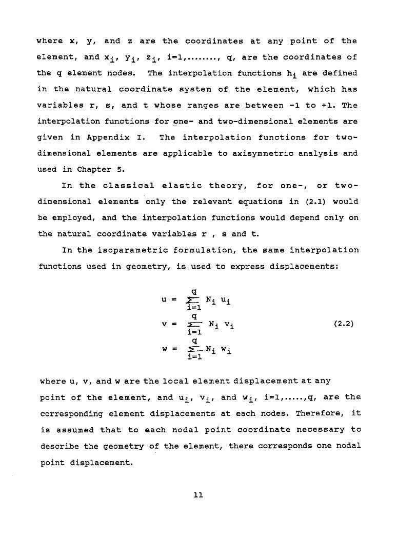
In the isoparametric formulation, the same interpolation
functions used in geometry, is used to express displacements:
where u, v, and w are the local element displacement at any
point of the element, and ui, vi, and wi, i=1, ,q, are the
corresponding element displacements at each nodes. Therefore, it
is assumed that to each nodal point coordinate necessary to
describe the geometry of the element, there corresponds one nodal
point displacement.
11

To obtain the derivatives of
chain rule:
one uses the
2.3 Finite-element matrices formulation
In general, the calculation of the element matrices should
be carried out in the global coordinate system, using global
displacement components if the number of natural coordinate
variables is equal to the number of global variables.
To evaluate the stiffness matrix of an element, one needs to
calculate the strain-displacement transformation matrix. The
element strains are obtained in terms of derivatives of element
displacements with respect to local coordinates. Because the
element displacements are defined in the natural coordinate
system using Eqn. (2.2), one has to relate the displacement with
repect to x, y, and z to the ones with respect to r, s, and t .
Let eqn (2.1) has the form
where f. denotes "function of ". The inverse relationship is
12
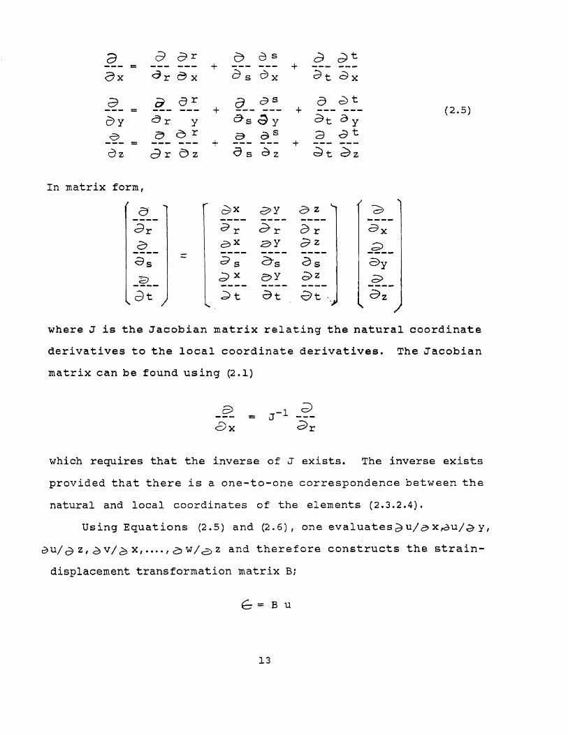
where J is the Jacobian matrix relating the natural coordinate
derivatives to the local coordinate derivatives. The Jacobian
matrix can be found using (2.1)
which requires that the inverse of J exists. The inverse exists
provided that there is a one-to-one correspondence between the
natural and local coordinates of the elements (2.3.2.4).
Using Equations (2.5) and (2.6), one evaluates u/ x, u/ y,
and therefore constructs the strain-
displacement transformation matrix B;
13

where u is a vector listing the element nodal point displacement
of Equation (2.2).
The element stiffness matrix corresponding to the local
element degree of freedom is
Here the elements of B are functions of the natural coordinates
r, s, and t. Therefore, the volume integration extends over the
natural coordinate volume, and the volume differential dv needs
also be written in the terms of the natural coordinates. In
general, we have
where detJ is the determinant of the Jacobin matrix in
Equation (2.7).
Since an explicit evaluation of the volume integral in Equation
(2.10) is not possible, numerical integration is used.
First, we rewrite Equation (2.9) in the form
where F = BT D B detJ and integration is performed in the
natural coordinate system of the element. F depends on r, s,
and t, but the actual functional relationship is, in general,
unknown. Using numerical integration, the stiffness matrix is now
where Fij k is the matrix F evaluated at point ri, s.Si'
and tk.
14

The sampling point ri, si t tk of the function and the
corresponding weighting factors ij k are chosen to obtain maximum
accuracy for the interval -1 to +1, and are as given in
Table [2.1].
The mass and load vectors are now given by
where H is a matrix of the interpolation functions. The above
matrices are evaluated using numerical integration.
To calculate the body force vector, RB , we use
For the surface force vector, we use F = H S fS detJ and for the
initial stress load vector we use F = BTJI detJ, and for the
mass matrix one has F = HT detJ. The weight coefficients
are the same as in the stiffness matrix evaluation and the same
order of numerical integration is used for different order,
values are obtained from the Table 2.1.
2.4 Convergence Considerations
The two requirements for monotonic convergence of a finite
element analysis are that the elements must be compatible and
complete. Completeness requires that the rigid body
displacements and constant strain states be possible [15].
15

TABLE 2.1
SAMPLING POINTS AND WE IN GAUSS—LEGENDRENUMERICAL INTEGRATION
n ri si
1 0. (15 zeros) 2. (15 zeros)
2 +0.57735 02691 89626 1.00000 00000 00000
3 +0.77459 66692 41483
+0.00000 00000 00000
0.55555 55555 55556
0.88888 88888 88889
4 +0.86113 63115 94053
+0.33998 10435 84856
0.34785 48451 37454
0.65214 51548 62546
Note : Sampling Points and Weights till Order 4 is given since thethesis involves integration upto order 3.
16

The necessity for the constant strain states can physically
be understood. When the limit as each element approaches a very
small size, the strain in each element approaches a constant
value, and any complex variation of strain within the structure
can be approximated. The requirement of compatibility means that
the displacements within the elements and across the element
boundaries must be continuous [15].
In the isoparametric formulation, one has the displacement
interpolation
which can be reduced to
17
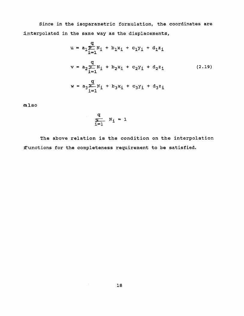
Since in the isoparametric formulation, the coordinates are
interpolated in the same way as the displacements,
The above relation is the condition on the interpolation
functions for the completeness requirement to be satisfied.
18

Chapter III
REVIEW OF MICROPOLAR ELASTICITY
3.1 Introductory Comments
A micropolar elastic material differs from classical elastic
material solids in that each point has extra rotational degree of
freedom independent of translation, and that a micropolar elastic
material can transmit couple stress as well as the usual force
stress [1].
The theory of micropolar elasticity is hoped to be
applicable to many new industrial materials with microstructures.
A dramatic increase in the applications of light-weight materials
in industry is expected in the future, thus enhancing the demand
of vast amounts of basic researches in the related area.
In this chapter, the micropolar elasticity theory is
reviewed. Erigen has studied a comprehensive recapulation of
micropolar elasticity theory based largely on earlier works by
him and his co-workers [4]. These equations are written in
rectangular cartesian tensor notation. His treatise provides an
excellent starting point for further investigations into linear
theory and is served as the main starting grounds for this study.
3.2 Basic Equations of Micropolar Elasticity
In 1964, Erigen and Suhubi first constructed the linear
theory of micropolar elasticity. The equilibrium equations of
micropolar elasticity is given [4]:
19

where ei km is the permutation tensor. Since only quasi-static
problems are considered in this study, the inertia terms can be
eliminated. The equilibrium equations thus become:
3.2.1 Constitutive equations
The linear forms of the stress and couple stress
constitutive equations for anisotropic micropolar elastic solids
are [1]:
is the microrotation vector and E rin is the Kronecker
delta. When the initial stress is zero, one has Akl = 0. Thus,
for the micropolar solid free of initial stress and couple
stress, we have
Various material symmetry conditions place further
restrictions on the constitutive coefficients Aklmn and Blkmn .
These restrictions are found in the same manner as in classical
20

elasticity [17]. If the body is isotropic with respect to both
force and couple stress, the solid is called isotropic. In this
case, the constitutive coefficients must be isotropic tensors.
For second and forth order isotropic tensors, one has the most
general forms:
where A, A1,....B2 and B 3 are functions of e- only. In this case,
Equations (3.4) and (3.5) take the special forms:
For vanishing initial stress A=O.
By introducing
the above equations can be rewritten as:
Isotropic micropolar elasticity can therefore be
distinguished from classical elasticity by the presence of four
extra elastic moduli; namely,
21

extra elastic moduli are set equal to zero, Equation (3.5) reduce
to the well-known Hooke's law of the linear isotropic classical
solid.
3.2.2 Restrictions on Micropolar Elastic Moduli
The necessary and sufficient conditions for the internal
energy to be non-negative are [2]:
The micropolar strain tensor indicates the relations among
the strain , displacement and microrotation. Since there are 33
equations with 33 variables, the formulation is therefore
complete.
3.2.3 Boundary conditions
Many different types of boundary conditions are suggested by
the nature of various applications. For example, one may
prescribe the displacement ui and microrotation on a boundary
surface s of a body [10]. Equally permissible is the alternate
prescription of the tractions and couples on s, i.e.
where t 1k and Ta lk are surface stress and surface couple
vectors, respectively, and t (n) K and m (n) K are the prescribed
tractions and couples on the bounding surface whose exterior is
22
unit normal vector n. In some other problems, it is possible to
prescribe the above two types of conditions as mixed boundary
conditions.
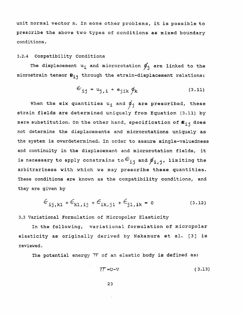
3.2.4 Compatibility Conditions
The displacement ui and microrotation φj are linked to the
microstrain tensor e ij through the strain-displacement relations:
When the six quantities ui and are prescribed, these
strain fields are determined uniquely from Equation (3.11) by
mere substitution. On the other hand, specification of eij does
not determine the displacements and microrotations uniquely as
the system is overdetermined. In order to assure single-valuedness
and continuity in the displacement and microrotation fields, it
is necessary to apply constrains to Є ij and φi,j, limiting the
arbitrariness with which we may prescribe these quantities.
These conditions are known as the compatibility conditions, and
they are given by
3.3 Variational Formulation of Micropolar Elasticity
In the following, variational formulation of micropolar
elasticity as originally derived by Nakamura et al. [3] is
reviewed.
The potential energy π of an elastic body is defined as:

where U is the strain energy and V is the work done by external
load acting on the body.
The principle of minimum potential energy claims, at the
equibrium states,
The work done by the body force Bi, body couple Ci, surface
traction Ti and surface couple Mi can be expressed as
Under virtual displacement and virtual microrotation, the
virtual work done by external load becomes
The equilibrium equations for Cosserat elasticity are given
in Equations (3.2):
Substituting the equilibrium equations into the above
24

equations, the first and second terms vanish, and the virtual
work becomes:
The strain energy for linear constitutive relation is
Then, we have a minimum potential energy functional of micropolar
elasticity:
3.4 Finite Element Formulation of Micropolar Elasticity
In this section, the finite element formulation for general
micropolar elasticity based on the previous section derived by
Nakamura et al. [12] is reviewed.
The total potential energy for a micropolar elastic solid
are:
Here tai and mji in the first term are the force stress and
couple stress, respectively; and
micropolar strain tensor and micro rotation gradient,
respectively. Bi and Ci in the second term are the applied body
25
force and body couple, respectively; and Ui and
displacement and microrotation for the i-direction, respectively.
Ti and Mi in the third term are the surface force and surface
couple tractions, respectively. The first two integrals are
volume integrals, while the last one is a surface integral for
which the surface traction and surface couples are prescribed.
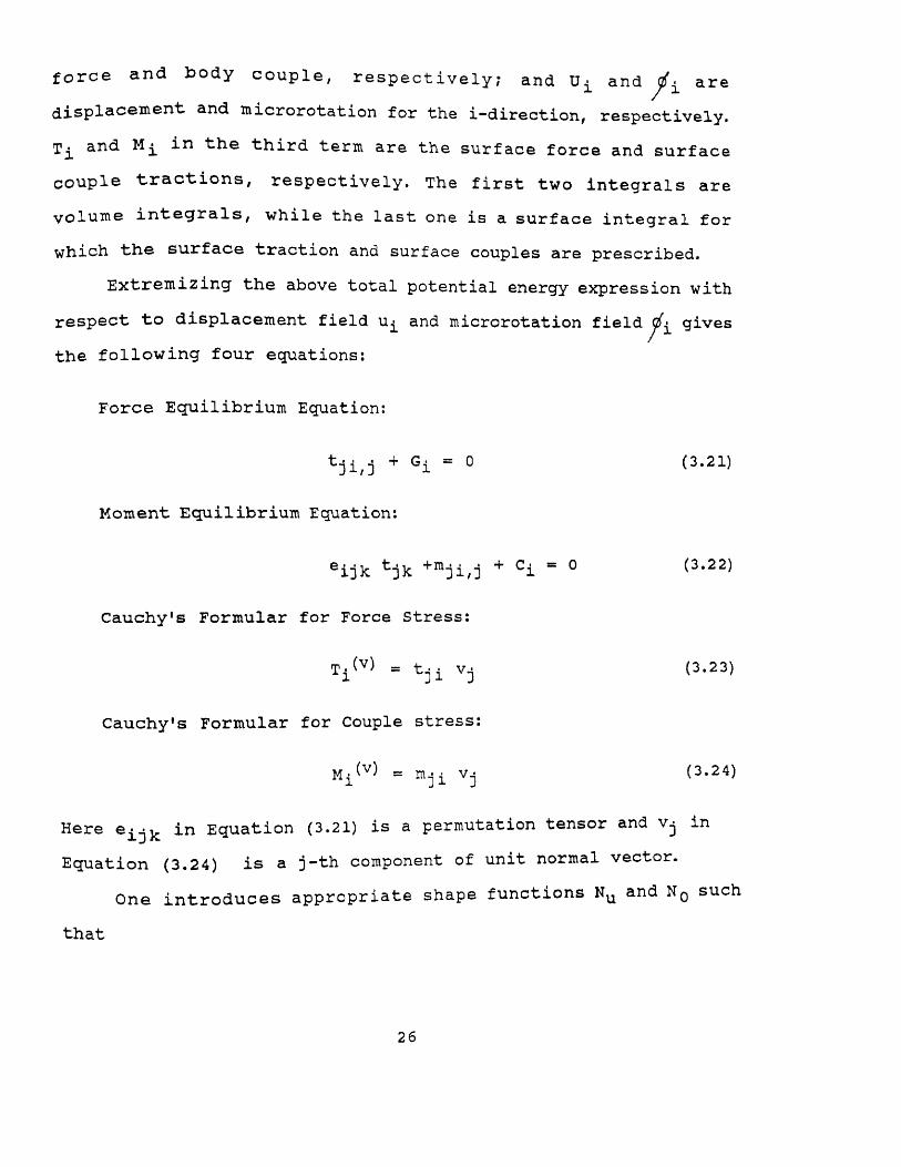
Extremizing the above total potential energy expression with
respect to displacement field ui and microrotation field
the following four equations:
Force Equilibrium Equation:
Moment Equilibrium Equation:
Cauchy's Formular for Force Stress:
Cauchy's Formular for Couple stress:
Here eijk in Equation (3.21) is a permutation tensor and vj in
Equation (3.24) is a j-th component of unit normal vector.
One introduces appropriate shape functions N u and N o such
that
26

Here u(x) and φ(x) are field variable vectors of displacement and
microrotation in the finite domain. U e and φeare nodal field
variable vectors corresponding to them. Using the expression for
micropolar strain tensor
where L is a differential operator and M is a permutation matrix,
and general constitutive equations
discretized equilibrium equation is obtained:
Here the nodal value vector is
the element stiffness matrix ke for micropolar elasticity is
are strain-displacement matrix and microrotation gradient matrix,
respectively.
27

CHAPTER IV
THREE-DIMENSIONAL ISOPARAMETRIC
ELEMENTS FOR MICROPOLAR ELASTICITY
4.1 Introductory Comments
Micropolar theory can be applied to many structure
materials, including fibrous, lattice and granular
microstructures [1]. Although numerous boundary value problems
have been solved analytically, the solutions are mainly limited
to the isotropic cases. Moreover, it is difficult to apply the
analytic methods to complex geometries. In addition, it is
generally difficult to solve analytically a three-dimensional
problem with the exception of a few special cases, such as the
stress and displacement boundary value problems with Volterra's
dislocation which can be treated as a plane problem and thus be
solved as a two-dimensional problem [18]. Thus finite element
methods are powerful tools for solving three-dimensional
micropolar elasticity problems with arbitrary geometries.
In this chapter, a general three-dimensional micropolar
elasticity theory in cylindrical system is reviewed first. A
general purpose three-dimensional finite element method is then
formulated, and a computer program is developed. The program is
used to solve a micropolar elastic cylinder with a semi-circular
groove under uniaxial tension.
4.2 General 3-D Micropolar Elasticity in Cylindrical coordinate
System
In this section, micropolar elasticity in Cartesian
28

Coordinate system is transformed into Cylindrical Coordinate
system.
Eringen's micropolar strain tensors
can be expressed in vector form:
where L is a gradient operator in Cartesian Coordinate (x,y,z):
Equation (3.11) can be transformed into cylindrical coordinate
system (r,e,z), using the gradient operator:
Thus
For Cylindrical Coordinate system (r,e,z) the constitutive
relationship has a form of:
29
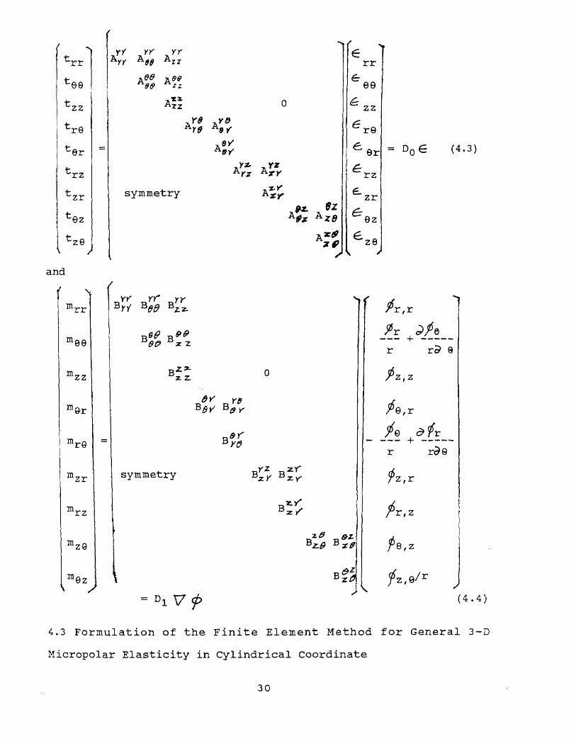
4.3 Formulation of the Finite Element Method for General 3-D
Micropolar Elasticity in Cylindrical Coordinate
30

In this section finite element method for 3-D micropolar
elasticity in cylindrical coordinate is derived.
The coordinates transformation from (x,y,z) to (r,θ,z) can
be calculated by using coordinate transformations:
The shape functions for the isoparametric element for eight
to twenty variable-number-nodes are discussed in detail in
Chapter 2. Using those shape functions Ni, displacement and
microrotation field inside each element can be interpolated:
Here q is a total number of the nodes of the element. For the
development of computer programs for 3-D micropolar elasticity,
only 8- and 20- node element are used in this study as described
in Chapter 2. uri, uθi and u z i are nodal displacements along x,
y,and z direction, respectively, and
31

microrotation about x, y, and z direction.
Defining the nodal value vector Ue, as
one can express Equation (14) in compact form:
and each shape function Ni are
expressed using natural coordinate system in each element.
The following shape functions are used for q = 8.
To calculate the derivatives with respect to the global
coordinate system, one needs coordinate transformation from
32

natural coordinate system to global coordinate system:
Here J is called Jacobian matrix defined by
Thus
33
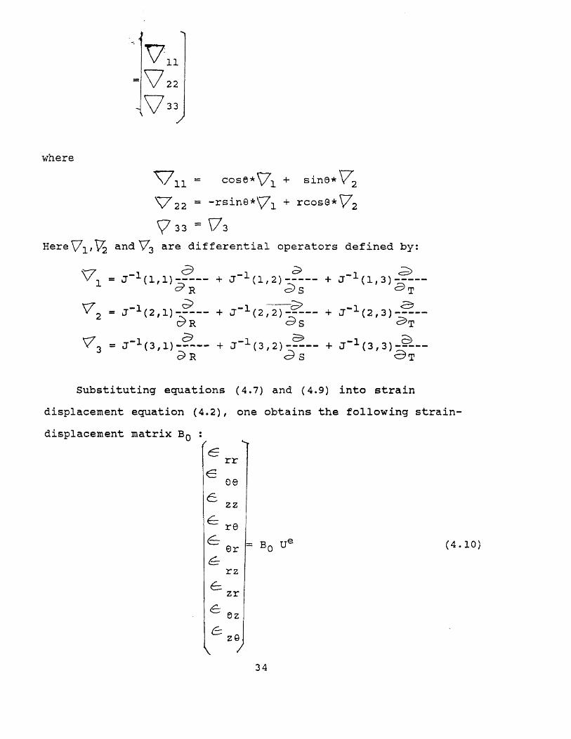
where
Substituting equations (4.7) and (4.9) into strain
displacement equation (4.2), one obtains the following strain-
displacement matrix B0 :
3 4

where
For the axisymmetric case,
Similary for microrotation gradient, one obtains the
following B 1 matrix:
35

where B 1 is a 9 by 48 matrics in q=8 case.
and
The B D - and B 1- matrices derived above can be substituted
into equation (3.29) to obtain element stiffness matrix k e. To
carry out volume integral of equation (3.29), numerical integration
of Gaussian quadrature shown in Table 2.1 is used in the program:
36

is the weighting factors of Gaussian Quadrature.
If body force is neglected, the force vector can becomes
The element stiffness matrices calculated in equation (4.12)
are assembled into a global stiffiness matrix in a symmetric
banded form with only the upper triangular part stored. Boundary
conditions of the prescribed displacements and microrotations are
imposed by modification of the corresponding rows and columns of
this global stiffness matrix. Similarly, the force vector is
37

generated by superposing element force vector in equation (4.13).
The linear algebraic equation is then solved for nodal
displacement using the skyline technique [12].
4.4 Numerical examples
The finite element formulations developed in the previous
section are implemented in Fortran programs (Appendix 2) with
either 8- or 20- node element, as shown Fig.4.1 and Fig. 4.2 The
eight nodes in the 8-node element represent the eight corners of
a cubic finite element, and the additional 12 nodes are included
in the 20- node element to bisect every two corners. In order to
verify the validity of the proposed finite element formulations,
two examples of axisymmetric micropolar elastic solids are
solved. The axisymmetric examples are deliberately chosen so that
they can be compared with existing two-dimensional analytical
solutions [ 10].
Example 1
This example is to solve a simple tension of cylindrical
Cosserat solids. The 8-node element is used. The finite
element meshes used are depicted in Fig.4.3 and Fig.4.4. The
material parameters are:
Coupling factor N=0.0, 0.25, 0.50, 0.7, 0.9, characteristic
length 1=8.333x10 -3 inch and Poissons ratio=0.3.
(psi), k=0.0 (psi)
(pound)
Dimensions used are: radius R=2 (inches) and length L=2
(inches).
38

Fig. 4.1 Eight Node Three-dimensional Element
39

Fig. 4.2 Twenty Node Three-dimensional Element
40

Fig.4.3. 8-Node Three-dimensional Element for Simple Tension.
41

Fig.4.4. 20-Node Three-dimensional Element for Simple Tension
42
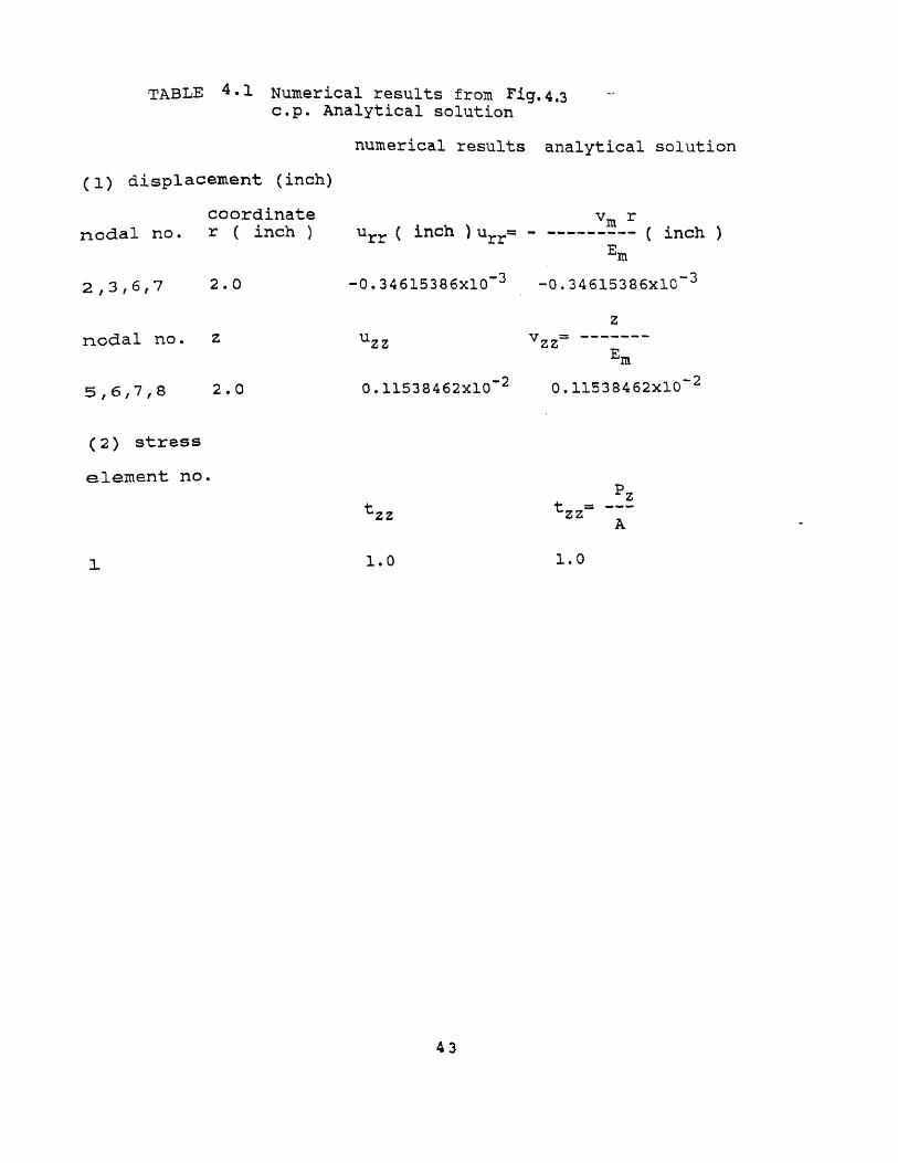
TABLE 4.1 Numerical results from Fig. 4.3 c .p . Analytical solution
numerical results analytical solution
43

TABLE 4.2 Numerical results from Fig. 4.4c.p. Analytical solution
numerical results analytical solution
44

The numerical results obtained in this study are summarized in
Table 4.1 and Table 4.2. Also shown in these tables are the
,analytical solutions of the same isotropic micropolar elastics
solids derived by Gauthier:
where A is the area of crossection and Young's modulus and
Poission's ratio are defined by
The significant findings are the following:
1. The numerical results for displacements are identical with
those from the analytical solution. This confirms the validity
of the proposed isoparametric finite element formulation.
2. The displacements are not effected by the coupling factor N.
This indicates that the micropolar effects do not affect the
simple test, meaning that during the simple test, micropolar
effects vanish.
3. The tension stress in the z-direction are found to be equal to
unity everywhere in every element.
Example 2
45
(1) The geometry is simple.
(2)The shape function and numerical integration are exact
for lower displacement field.
Example 2
To demonstrate the capability and validity of the proposed
finite element formulation, an isotropic micropolar elastic
cylinder with a semi-circular groove is used as the second
example. To the best of the author's knowledge, this particular
problem has never been solved before, probably due to the
difficulty in obtaining analytical solutions with such a complex
geometry . In the following it is shown that the numerical
results obtained in this study indeed coincides with the
available experimental results when the coupling factor is equal
to zero, i.e., when the micropolar solid reduces to a classical
material.
The isotropic micropolar elastic cylinder with a semi-
circular groove used in this example is shown in Fig.4.5. The
diameter of the cylinder D is fixed to 0.1 inch. The radius
ratio k is defined by k = r/d, where r is the radius of groove,
and d is D - 2r. In this study, k is varied in the range of 0.05
to 0.5. Finite element mesh used for the analysis is shown in
Fig.4.6 for radius ratio k=0.5. The material properties used for
the isotropic case are as listed in Table.4.3. The characteristic
length 1 is fixed to 8.333x10 -3 , and the Poisson ratio of 0.3 is
used. These properties are summarized in Table 4.3.
The numerical results of Kc , or sigma max/sigma nom,
46
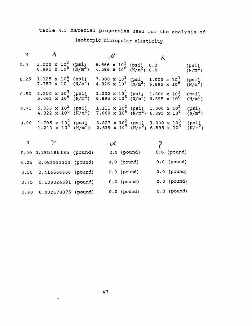
Table 4.3 Material properties used for the analysis of
isotropic micropolar elasticity
N λ µ κ
0.0 1.000 x 10³(psi)6.895 x 10⁶ (N/m2)
6.666 x 10² (psi)4.596 x 10⁶ (N/m2)
0.0 (psi)0.0 (N/m2)
0.25 1.125 x 10⁴ (psi)
7.757 x 10⁷ (N/m2)7.000 x 10 3 (psi)4.826 x 10 7 (N/m2)
1.000 x 10 3 (psi)6.895 x 10 6 (N/m2)
0.50 2.250 x 10³(psi)5.063 x 10⁶ (N/m2)
1.000 x 10 3 (psi)6.895 x 10⁶ (N/m2)
1.000 x 10 3 (psi)6.895 x 10 6 (N/m2)
0.75 5.833 x 10 2 (psi)4.022 x 10 6 (N/m2)
1.111 x 10 2 (psi)7.660 x 10 6 (N/m2)
1.000 x 10³ (psi)6.895 x 10⁶ (N/m2)
0.90 1.795 x 10 2 (psi)1.213 x 10 6 (N/m2)
3.827 x 10 2 (psi)2.639 x 10⁵ (N/m2)
1.000 x 10 3 (psi)6.895 x 10 6 (N/m2)
N γ α β
0.00 0.185185185 (pound) 0.0 (pound) 0.0 (pound)
0.25 2.083333333 (pound) 0.0 (pound) 0.0 (pound)
0.50 0.416666666 (pound) 0.0 (pound) 0.0 (pound)
0.75 0.108024691 (pound) 0.0 (pound) 0.0 (pound)
0.90 0.032578875 (pound) 0.0 (pound) 0.0 (pound)
.47

Fig. 4.5 Isotropic Micropolar Elastic Cylinder with Semi-
circular Groove
48

Fig.4.6 Finite element meshes
49

Table 4.4 Numerical results of stress concentration factor
vs r/d. (
stress )
isotropic for force stress and couple
ratio N=0.90 N=0.75 N=0.50 N=0.25 N=0.00r/d
0.05 1.75 1.92 2.26 2.58 2.73
0.08 1.65 1.81 2.11 2.40 2.53
0.10 1.60 1.75 2.03 2.28 2.39
0.13 1.53 1.67 1.91 2.13 2.22
0.17 1.47 1.59 1.80 1.98 2.04
0.20 1.43 1.54 1.73 1.88 1.93
0.23 1.40 1.50 1.66 1.79 1.84
0.27 1.36 1.45 1.60 1.70 1.74
0.30 1.33 1.42 1.55 1.65 1.68
0.35 1.28 1.35 1.47 1.56 1.59
0.40 1.25 1.31 1.42 1.49 1.52
0.45 1.23 1.29 1.38 1.44 1.46
0.50 1.20 1.26 1.34 1.40 1.42
50

Fig. 4.7 Stress Concentraction Factor, K c for a Round Tension
Bar with a Semi-circular Groove in Three-dimensional
case ( Orthotropic for Force Stress and Couple Stress)
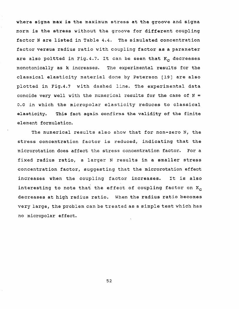
where sigma max is the maximum stress at the groove and sigma
norm is the stress without the groove for different coupling
factor N are listed in Table 4.4. The simulated concentration
factor versus radius ratio with coupling factor as a parameter
are also poltted in Fig.4.7. It can be seen that K c decreeses
monotonically as k increases. The experimental results for the
classical elasticity material done by Peterson [19] are also
plotted in Fig.4.7 with dashed line. The experimental data
concide very well with the numerical results for the case of N =
0.0 in which the micropolar elasticity reduces to classical
elasticity. This fact again confirms the validity of the finite
element formulation.
The numerical results also show that for non-zero N, the
stress concentration factor is reduced, indicating that the
microrotation does affect the stress concentration factor. For a
fixed radius ratio, a larger N results in a smaller stress
concentration factor, suggesting that the microrotation effect
increases when the coupling factor increases. It is also
interesting to note that the effect of coupling factor on K c
decreases at high radius ratio. When the radius ratio becomes
very large, the problem can be treated as a simple test which has
no micropolar effect.
52

CHAPTER V
AXISYMMETRIC ELEMENTS
5-1 Introductory Comments
Many engineering problems involve solids of revolution
subjected to axially asymmetric loading. It is therefore
important to consider the asymmetric problems in the micropolar
elasticity. The axisymmetric problems can be transformed to a
two-dimensional plane case and solved by two-dimensional
analytical methods. However, no universal technique is available
for general boundary value problems, making the solutions
procedure tedious. In this chapter it is demonstrated that the
finite element method can overcome these short-comings by
offering a general-purpose numerical solution, thus providing a
powerful technique in solving axisymmetrical problems.
In the following sections, the simplified two-dimensional
strain-displacement relationship for micropolar elasticity of the
axisymmetric case due to axisymmetric load is derived, and then
the isoparametric finite element method is applied to formulate
the simplified strain-displacement relationship. Isoparametric
elements of 4-node and 8-node are used. The programming
organization is then described. The program is also verified by
comparing the numerical results with analytical solutions for
simple tension of cylindrical Cosserat solid and also for stress
concentration of a round bar with semi-circular groove.
5.2 Axisymmetric Micropolar Elasticity
To derive the simplifed two-dimensional strain-displacement
53

relationship for micropolar elasticity of the axisymmetric
material properties under axisymmetric loading, one starts with
micropolar strain tensors defined in Equation. 3.11.
This equation was transformed intothe cylindrical
coordinate system (r,o,z) in chapter 4 and had the form:
For the axisymmetric case, dependency on e- vanishes and the
above strain tensors reduce to the following form:
In the case of axisymmetric load, microrotations about r and
z axis vanish, thus Equation (5.1) can be further reduced :
54

From now on, the following simplified notations are used.
Thus expression (5.2) becomes
The above kinematical considerations tell one that for
elastic solids under axisymmetric loading, each material point
has only three degrees of freedom, i.e., (u,v,φ), which represent
displacements in the r, and z directions; and microrotation about
0 direction, respectively.
5.3 Axisymmetric Element:
The shape functions for the isoparametric element for four
to nine variable-number-nodes were discussed in chapter 3, and
also shown in Appendix 1. Using those shape functions Ni,
displacement and microrotation field inside each element can be
interpolated:
55

Here q is the total number of nodes of the element and q= 4 or 8
For the development of the computer program for micropolar
elasticity, both 4 node- and 8 node-element are used . u i and vi
are nodal displacements along r and z direction, respectively;
is a nodal microrotation about e direction.
By defining the nodal value vector U e :
and each shape function Ni are expressed using natural
coordinate system in each element. The following shape functions
To calculate the derivatives with respect to global
coordinate system, one needs coordinate transformation:
56

Here J is the Jacobian matrix and is defined by
thus
By substituting Equations ( 5.5) and (5.6) into strain
displacement equation (5.3), one obtains the following strain-
displacement matrix B o :
57

Similarly for microrotation gradient, one obtains the
following B1 matrix:
58

The B o - and B 1 - matrices derived above can be substituted
Into equation (3.29) to obtain the element stiffness matrix k e.
To carry out volume integral of Equation (3.29), numerical
integration of Gaussian quadrature is used in the program. The
sampling points and weighting factors for the interval -1 to +1
are given in Table 2.1.
If body force is neglected, the force vector of equation
(3 .28)) becomes
59
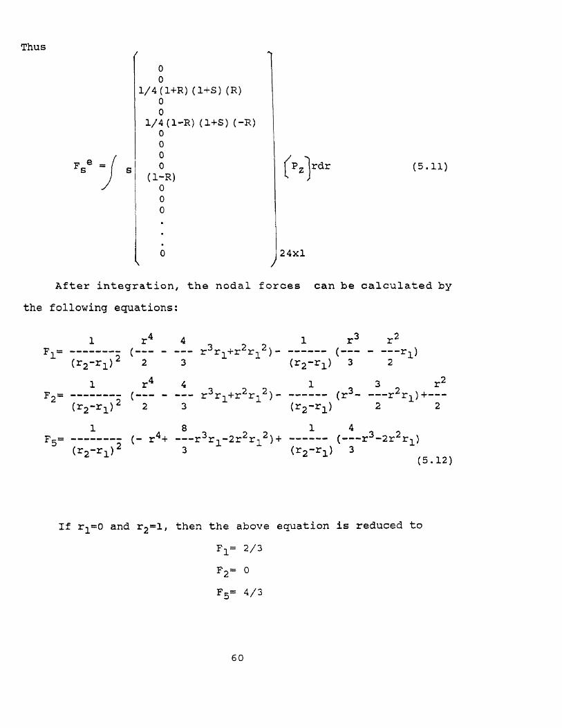
Thus
After integration, the nodal forces can be calculated by
the following equations:
60
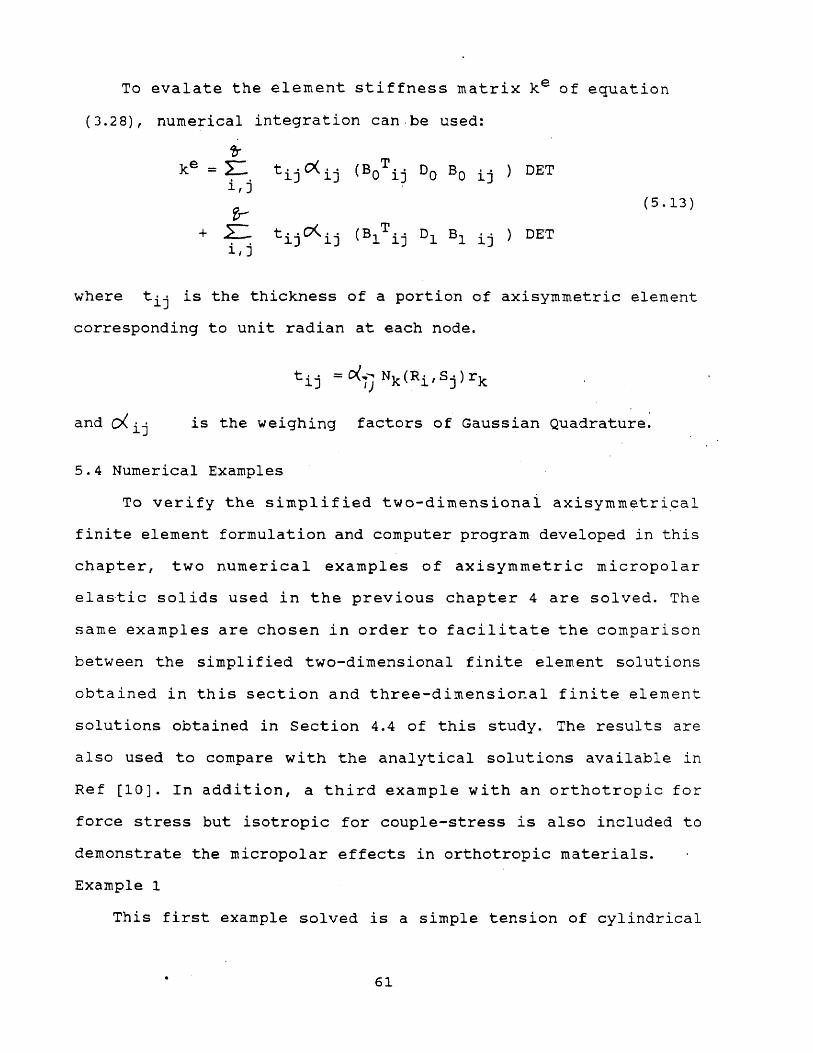
To evalate the element stiffness matrix ke of equation
(3.28), numerical integration can be used:
where tip is the thickness of a portion of axisymmetric element
corresponding to unit radian at each node.
is the weighing factors of Gaussian Quadrature.
5.4 Numerical Examples
To verify the simplified two-dimensional axisymmetrical
finite element formulation and computer program developed in this
chapter, two numerical examples of axisymmetric micropolar
elastic solids used in the previous chapter 4 are solved. The
same examples are chosen in order to facilitate the comparison
between the simplified two-dimensional finite element solutions
obtained in this section and three-dimensional finite element
solutions obtained in Section 4.4 of this study. The results are
also used to compare with the analytical solutions available in
Ref [10]. In addition, a third example with an orthotropic for
force stress but isotropic for couple-stress is also included to
demonstrate the micropolar effects in orthotropic materials.
Example 1
This first example solved is a simple tension of cylindrical
61

Cosserat solids as used in Chapter 4. Both 4- and 8-node
elements are used in this study for comparison. As shown in
Fig.5.1 and Fig.5.2, the four corner nodes in a 8-node element
correspond with the four nodes in a 4-node element. The finite
element meshes used is shown in Fig.5.1 and Fig.5.2. The material
parameter used are: Coupling factor N=0.0, characteristic length
1=8.333x10 -3 inch and Poissons ratio=0.3.
k=0.0 (psi),
Dimensions are: radius R=2 (inches) and length L=2 (inches).
The r- and z-displacements obtained by two-dimensional numerical
simulations in this study are summarized in Table 5.1 and Table
5.2, for the 4- and 8-node rectangular element, respectively.
Again it is found that the displacements are independent of the
coupling factor for axisymmetrical loading. It can also be seen
that the displacements at the four corner nodes of the 8-node
element (Table. 5.2) also coincide with the three-dimensional
simulations obtained with a 20-node three-dimensional element in
the previous chapter( Table 4.2), and the 4-node two-dimensional
results (Table 5.1) coincides with the 8-node three-dimensional
results in Table 4.1. These results also coincide with Gauthier's
analytical solution shown in those tables. All these confirm the
adequacy and validity of the proposed finite element approach.
To confirm the applicability of the proposed finite element
method to an arbitrary geometry, a patch test problem as defined
in Fig.5. 3 for 4-node and 8-node elements, respectively are
performed. Five elements are assembled as shown in Fig.5.3 and
subjected to an axial tension. The boundary conditions are
62
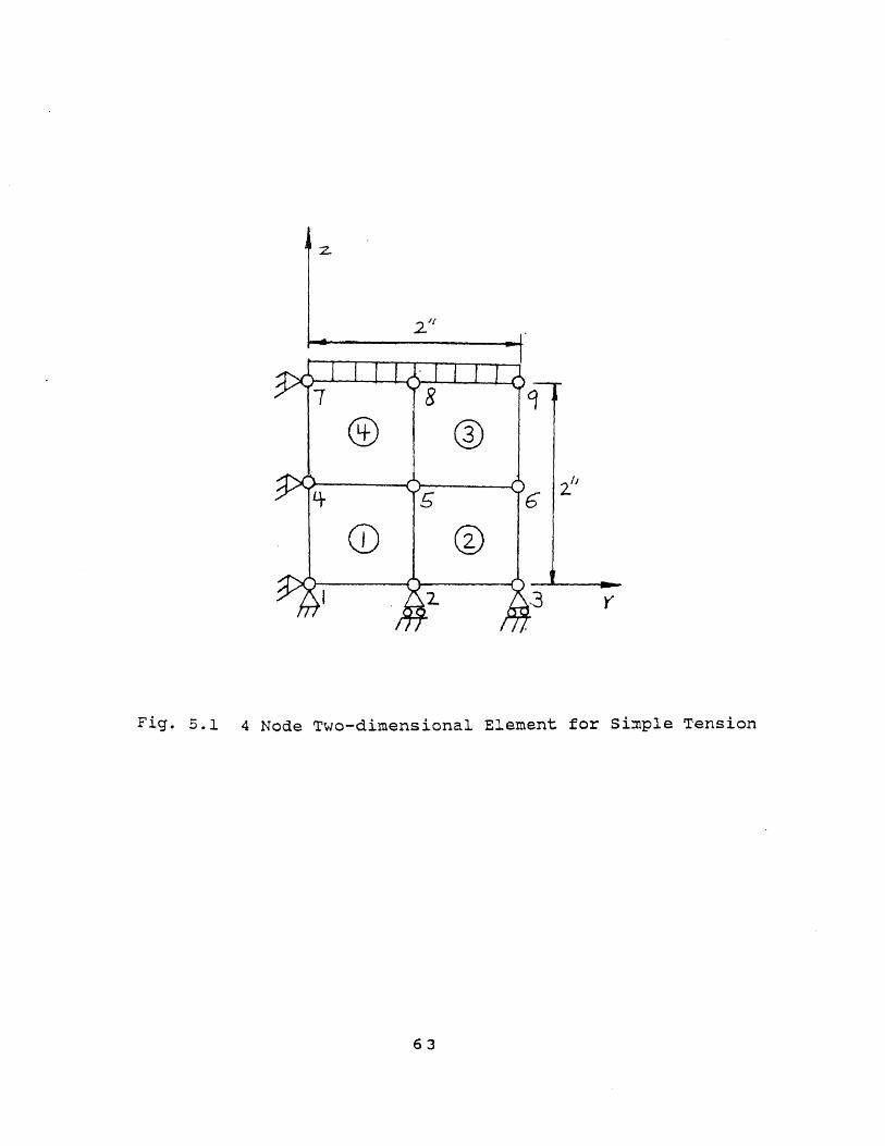
Fig. 5.1 4 Node Two-dimensional Element for Simple Tension
63

Fig. 5.2 8 Node Two-dimensional Element for Simple Tension
64
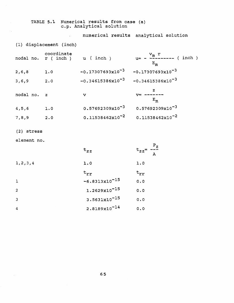
TABLE 5.1 Numerical results from case (a)c.p. Analytical solution
numerical results analytical solution
65

TABLE 5.2 Numerical results from case (b)c.p. Analytical solution
numerical results analytical solution
66
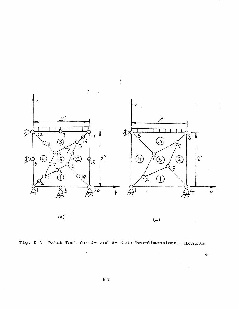
Fig. 5.3 Patch Test for 4- and 8- Node Two-dimensional Elements
6 7

TABLE 5.3 Numerical results from case (a)c.p. Analytical solution
numerical results analytical solution
(1) displacement (inch)
68
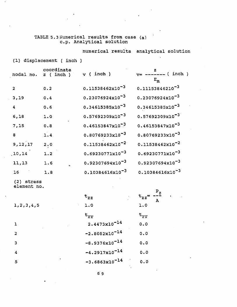
TABLE 5.3 Numerical results from case (a)c.p. Analytical solution
numerical results analytical solution
6 9

TABLE 5 .3 Numerical results from case (b)c.p. Analytical solution
numerical results analytical solution
0

specified in Fig. 5.3 the numerical results are summarized in
Table 5.3 and Table 5.4 , for 4-node and 8-node patch elements,
respectively. These results are found to be exactly identical
with those obtained with rectangular element, confirming the
applicability to an arbitrary geometry with the isoparametric
finite element.
Example 2
The second example solved by the simplified two-dimensional
method is an isotropic micropolar elastic cylinder with a semi-
circular groove shown in the inset of Fig.5.4, subjected to an
axisymmetric loading. The same example is solved in Chapter 4 by
three-dimensional method. The material properties and
geometrical dimensions are as given in Table 4.3 . Numerical
results for different coupling factor N are listed in Table 5.4 ,
and ploted in Fig.5.4. Again these results coincide exactly with
the three-dimensional finite element results shown in Table 4.4.
The experiment results from the literature for the classical
material (N=0.0) are also plotted in the same figue which dased
line. One can see excellent agreement.
71

Table 5.4 Numerical results of stress concentration factor
vs r/d. ( isotropic for force stress and couple
stress )
ratior/d
N=0.90 N=0.75 N=0.50 N=0.25 N=0.00
0.05 1.75 1.92 2.26 2.58 2.73
0.08 1.65 1.81 2.11 2.40 2.53
0.10 1.60 1.75 2.03 2.28 2.39
0.13 1.53 1.67 1.91 2.13 2.22
0.17 1.47 1.59 1.80 1.98 2.04
0.20 1.43 1.54 1.73 1.88 1.93
0.23 1.40 1.50 1.66 1.79 1.84
0.27 1.36 1.45 1.60 1.70 1.74
0.30 1.33 1.42 1.55 1.65 1.68
0.35 1.28 1.35 1.47 1.56 1.59
0.40 1.25 1.31 1.42 1.49 1.52
0.45 1.23 1.29 1.38 1.44 1.46
0.50 1.20 1.26 1.34 1.40 1.42
72

Fig. 5.4 Stress Concentraction Factor, Kc for a Round Tension
Bar with a Semi-circular Groove in Three-dimensional
case ( Orthotropic for Force Stress and Couple Stress)
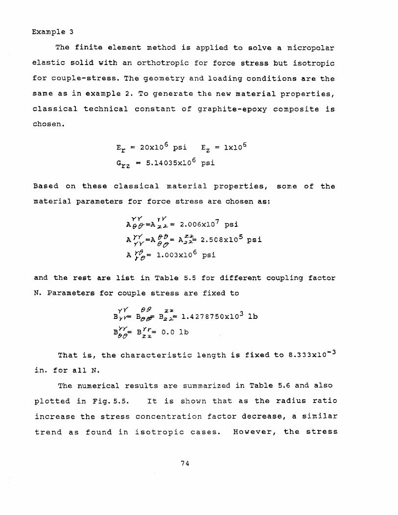
Example 3
The finite element method is applied to solve a micropolar
elastic solid with an orthotropic for force stress but isotropic
for couple-stress. The geometry and loading conditions are the
same as in example 2. To generate the new material properties,
classical technical constant of graphite-epoxy composite is
chosen.
Based on these classical material properties, some of the
material parameters for force stress are chosen as:
and the rest are list in Table 5.5 for different coupling factor
N. Parameters for couple stress are fixed to
That is, the characteristic length is fixed to 8.333x10 3
in. for all N.
The numerical results are summarized in Table 5.6 and also
plotted in Fig.5.5. It is shown that as the radius ratio
increase the stress concentration factor decrease, a similar
trend as found in isotropic cases. However, the stress
74

Table 5.5 SOME OF MATERIALS PARAMETERS TO FORCE STRESS
OF ANISOTROPIC MATERIALS

Table 5.6 Numerical results of stress concentration factor
vs r/d. ( othotropic for force stress isotropic
isotropic for couple stress )
ratior/d
N=0.90 N=0.75 N=0.50 N=0.25 N=0.00
0.05 1.77 1.90 2.24 3.10 3.73
0.08 1.67 1.81 2.14 3.08 3.81
0.10 1.62 1.76 2.08 3.02 3.79
0.17 1.48 1.61 1.89 2.77 3.59
0.23 1.40 1.51 1.77 2.58 3.35
0.30 1.34 1.43 1.66 2.38 3.06
0.40 1.27 1.35 1.55 2.15 2.68
0.50 1.23 1.30 1.46 1.97 2.36
76
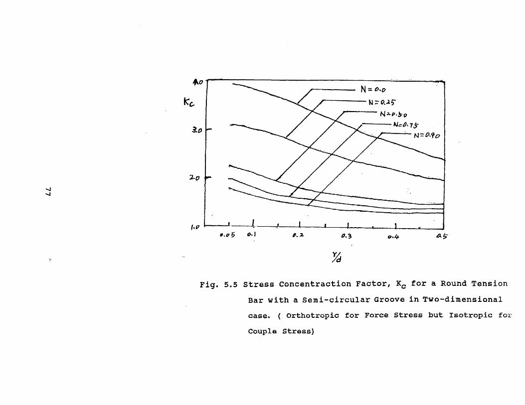
Fig. 5.5 Stress Concentraction Factor, K c for a Round Tension
Bar with a Semi-circular Groove in Two-dimensional
case. ( Orthotropic for Force Stress but Isotropic for
Couple Stress)

concentraction factor for a fixed N are higher than that in the
isotropic cases.
78
CHAPTER VI
CONCLUSION
6.1 Concluding Remarks
In this study isoparametric finite element method for
isotropic and orthotropic axisymmetric micropolar (Cosserat)
elastic solids was developed. Both 8- and 20-node elements were
employed for solving general three-dimensional problems, and both
4- and 8-node elements were used for two-dimensional cases. Both
three-dimensional and two-dimensional finite element formulation
for cylindrical coordinate system were obtained. Corresponding
Fortran programs were developed to solve several two-dimensional
and three-dimensional problems for micropolar elastics solids.
The validity and compatibility of the developed three-
dimensional finite element programs were established by comparing
the numerical results with available analytical solutions for a
cylindrical Cosserat solid subjected to a simple tension. The
numerical results for displacements were found to be identical
with the analytical solutions, and the displacements was
independent of the coupling factor. The flexibility and
capability of the three-dimensional finite element method are
then demonstrated by solving the stress concentration for a
classical round tension bar with a semi-circular groove subjected
to an axial symmetrical load. For the first time, to the best
of the author's knowledge, the effects of various coupling factor
on stress concentration factor were obtained for the micropolar
round tension bar with a semi-circular groove subjected to an
79

axial symmetrical load. The stress concentration factor on the
micropolar elastic solids was smaller than that in classical
elastic solids for the same radius ratio. The stress
concentration factor was also found to decrease monotonically as
radius ratio increases. Again the validity and compatibility
are confirmed by the excellent fit between the available
experimental data for classical materials and the numerical
results at zero coupling factor, as microelasticity reduces to a
classical case when the coupling factor N is equal to zero. In
the classical case, the effects of microrotation is vanished.
The three-dimensional finite element formulations can be
simplified to a two-dimensional formulation in the case of an
asymmetric object when subjected to an axisymmetric load, and can
result in significant savings in CPU time. The simplified two-
dimensional programs with both 4- and 8-node elements are first
applied to solve the simple tension of a cylindrical Cosserat
solid, - which has also been solved by the three-dimensional
programs in this study. It is found that the displacements at
the four corner-nodes of the 8-node element coincides exactly
with those obtained by the 4-node element, indicating the
adequacy of the 4-node element approach, which is more economic
in CPU time. In addition, the 8-node two-dimensional simulation
results are also identical with the three-dimensional simulation
results obtained with a 20-node three-dimensional element in this
study; and the 4-node two-dimensional numerical results are
identical with those with 8-node three-dimensional results in
this study.
80

The simplified programs are also applied to solve a
micropolar elastic solid with a semi-circular-groove subjecting
to an axial symmetrical loading. Again the results coincide
exactly with the three-dimensional finite element results, as
well as the experimental data for the special case when the
coupling factor is reduced to zero. The applicability of the
proposed finite element method to an arbitrary geometry is also
verified by the patch tests performed on a two-dimensional
example. The results are found to be exactly identical with
those obtained with the rectangular elements. Finally, the
developed two-dimensional finite element formulation is applied
to investigate the dependency of material properties for a
material with an orthotropic for stress but isotropic for couple
stress. It was verified that the new material depicts a similar
trend as the isotropic material with the stress concentration
factor decreases with increasing radius ratio. However, the
stress concentration factor is larger for any particular coupling
factor.
6.2 Future Study
Another interesting topic is the boundary value problem for
the stress concentration at spherical cavity in a field of
isotropic tension. This is solved by Bleustein [20] using the
theory developed by Mindlin. It is found that the stress
concentration factor is larger than the 3/2 of classical
elasticity for a wide range of material properties and ratio of
radius of cavity to a length parameter of the material with a
critical ratio, nearly independent of the remaining material
81

properties, for which the stress concentration factor is a
maximum. Bleustein found that for the classical theory of
elasticity the stress concentration factor is a constant,
independent of material properties and the radius of cavity.
However, the solution obtained by the theory of micropolar
elasticity shows a stress concentration factor which depends on
both material properties and radius. The stress concentration
factor is higher than the classical value of 3/2. It is
generally true that when the micropolar behavior is considered
stress concentration factor becomes smaller than the classical
elasticity. Therefore identifying the condition under which the
stress concentration factor is larger than the classical
elasticity is an interesting future study.
82

REFERENCES
[1] W. Voig, "Theoretische studien uber die
elasticitutsverhultnisse der krystalle," Abhandlungen der
koniglichen gesllschaft der wissenshaften zu gottingen,
vol. 24, Gottingen, 1987.
[2] E. and F. Cosserat, Theorie des corps deformables, Paris, A.
Hermann and Sons, 1909.
[3] S. Nakamura, R. Bendic and R. Lakes, Finite Element Method
for Othotropic Micropolar Elasticity. Int. J. Engng Sci.
Vol. 22, No.3, 1984, pp. 319-330.
[4]A. C. Eringen and E. S. Suhubi, " Nonlinear Theory of Simple
Micro-elastic Solid-I," Int. J. Engng. Sci, Vol. 2, 1964,
pp. 189-203.
[5] R. D. Mindlin, " Micro-structure in linear Elasticity,"
Arch. Rat. Mech. Anal., Vol. 16, 1984, pp. 51-78.
[6] R. D. Mindline and H. F. Tiersten, " Effects of Couple-
stress in linear Elasticity, " Arch. Rat. Mech. Anal. Vol.
11, 1962, pp. 415-448.
[7] T.Ariman, On circular Micropolar Plates, Ingenieur Archir.
Vol. 37, 1968, pp. 156-160.
[8] R. N. Kaloni and T. Ariman, " Stress Concentration Effects
in Micropolar Elasticity," ZAMP, Vol. 18, 1967, pp. 130-141.
[9] M.Kishida,K.Sasaki, H. Hanzawa, One Solution of Three-
dimensional Boundary Value Problems in The Couple-stress
Theory of Elasticity. A.S.M.E. J. of Applied Mechanics,
Vol.49, 1982, pp. 519-524.
[10] R. D. Gauthier, Analytical and Experimental Investigations
83

in Linear Isotropic Micropolar Elasticity. doctoral
dissertation, Univ. of Colorado, 1974.
[11] R.D.Gauthier and W. E. Jahsman, A Quest for Micropolar
Elastic Constants, J. of Applied Mechanics, June 1975, pp.
369-374.
[12] S. Nakamura and Y. Z. Jen
[13] S. Nakamura, Internal Report 1.
[14] S. Nakamura, Internal Report 2.
[15] K.J.Bathe, Finite Element Procedures in Engineering
Analysis. Prentice-Hall, Inc., 1982.
[16] 0. Ural, Matrix methods and use of Computers in Structural
ngineering, Intext Educational Publishers, NY, 1971.
[17] S. P. Timoshenko and J. N. Goodier, Theory of Elasticity,
3rd ed., NY, Mcgraw-Hill, 1970.
[18] B. M. Chiu and James D. Lee, On the Plane Problem in
Micropolar Elasticity, Int. J. Engng. Sci., Vol 11, 1973,
pp. 997-1012.
[19] R. E. Peterson, Stress Concentraction factor, John-Willy &
Sons, 1974.
[20] J. L. Bleustein, " Effects of Micro-Structure on The Stress
Concentration at a Spherical Cavity", Int. J. Solids
Structure, Vol. 2, 1966, pp. 83-104.
84

APPENDIX I
Interpolation Functions of Four to Eight Variable -
Number-Nodes Two-Dimensional Element
(a) Four to 8 variable-number-nodes two-dimensional element
Include only if node is defined
85
APPENDIX II Program Listing for Two and Three-dimensional Isoparametric Finite Elements
C 3-D MICROPOLAR FINITE ELEMENT METHODC
IMPLICIT REAL*8(A-H2O-Z)INTEGER*4 ITIMINTEGER*2 TYPE,CODECOMMON/B01/B0(200,9,48),B1(200,9,48),INXY(200),ID(300)COMMON/XYZ/NNP(200,8),X(300),Y(300),Z(300)COMMON/CSTRN/KSTRN(1000),KSTRT(1000)COMMON/MAT/D0(9,9),D1(9,9),A11,Al2,A22,A23,811COMMON/AIN/NB,NC,ND,NE,NN,TH,NINT,R,S,T,DETCOMMON/FSK/A(350000) ,V(1800) ,EK(48,48) ,MAXA(1801) ,NEIREREAD(5,100) NE
100 FORMAT(I4)DO 10 N=1,NEREAD(5,200) (NNP(N,I),I=1,8),INXY(N)
200 FORMAT(4X,8I4,3X,I5)10 CONTINUE
READ(5,100) NNDO 20 N=1,NNREAD(5,300) X(N),Y(N),Z(N)
20 CONTINUE300 FORMAT(4X,3F20.10)
READ(5,100) NCDO 30 N=1,NCREAD(5,400) KSTRN(N),KSTRT(N)
400 FORMAT(4X,I4,i7)30 CONTINUE
READ(5,550)NINT550 FORMAT(I5)
READ(5,600)A11,Al2,A22,A23,B11600 FORMAT(5E20.7)
WRITE(6,610)A11,Al2,A22,A23,B11610 FORMAT(2X,'A11=',E20.7,°Al2=',E20.7,1A22=1,
*E20.7,'A23=',E20.7,'B11=',E20.7)ND=NN*6NB=0DO 40 IB=1,NEIMAX=MAXO(NNP(IB,1),NNP(IB,2),NNP(IB,3),NNP(IB,4),NNP(IB,5),*NNP(IB,6),NNP(IB,7),NNP(IB,8))IMIN=MINO(NNP(IB,1),NNP(IB,2),NNP(IB,3),NNP(IB,4),NNP(IB,5),*NNP(IB,6),NNP(IB,7),NNP(IB,8))NBCHEK=(IMAX-IMIN+1)*6IF(NBCHEK.GT.NB) NB=NBCHEKIF(NB .GT. 300) GO TO 99
40 CONTINUESCALE=1.0D0DO 41 I=1,NNX(I)=X(I) *SCALEY(I)=Y(I) *SCALE
41 Z(I)=Z(I)*SCALE
86

WRITE(6,700)700 FORMAT(1H1)
WRITE(6,800)800 FoRmAT(3x,1*****************************************************1****************1)WRITE(6,900)
900 FORMAT(3X,'*',68X,'*')WRITE(6,1000)
1000 FORMAT(3X,140,13X,'3-D ORTHOTROPIC MICROPOLAR STRESS ANALYSIS',13X,'*')
WRITE(6,1050)1050 FORMAT(3X,'*',28X,' SKYLINEMICRO',27X,'*')
WRITE(6,900)WRITE(6,800)WRITE(6,1100)
1100 FORMAT(/20X,'**** DISCRETIZATION NUMBER ****')WRITE(6,1200)
1200 FORMAT(/13X,'ELEMT.#'13X,'NODES.P,3X,'CONSTR.#1,3X,'THIKNES',3X,'BAND-WIDTH',3X,'GAUSS NUMERICAL INTEGRATION ORDER')
WRITE(6,1300) NE,NN,NC,TH,NB,NINT1300 FORMAT(13X,I4,7X,I3,7X,I3,5X,E10.3,5X,I5,19X,I2)
WRITE(6,1700)1700 FORMAT(//21X,'**** ELEMENT-NODE CONNECTION ****')
WRITE(6,1800)1800 FORMAT(/3X,IELM NP1 NP2 NP3 NP4 NP5 NP6 NP7 NP8 IXY ELM
* NP1 NP2 NP3 NP4 NP5 NP6 NP7 NP8 IXY')DO 45 I=1,NE
45 ID(I)=ILINE=NE/2IRESID=NE-2*LINEDO 50 N=1,LINE
50 WRITE(6,1900) (ID(2*(N-1)+I),NNP(2*(N-1)+I,1),NNP(2*(N-1)+I,2),*NNP(2*(N-1)+I,3),NNP(2*(N-1)+I,4),NNP(2*(N-1)+I,5),*NNP(2*(N-1)+I,6),NNP(2*(N-1)+I,7),NNP(2*(N-1)+I,8),*INXY(2*(N-1)+I),I=1,2)
1900 FORMAT(2(2X,I4,1X,I3,1X,I3,1X,I3,1X,I3,1X,I3,1X,I3,1X,I3,1X,I3,*1X,I6))IF(IRESID .EQ. 0) GO TO 56WRITE(6,1900) (ID(2*LINE+I),NNP(2*LINE+I,1),NNP(2*LINE+I,2),*NNP(2*LINE+I,3),NNP(2*LINE+I,4),NNP(2*LINE+I,5),NNP(2*LINE+I,6),*NNP(2*LINE+I,7),NNP(2*LINE+I,8),INXY(2*LINE+I),I=1,IRESID)
56 WRITE(6,2000)2000 FORMAT(//24X,'**** NODAL COORDINATE ****')
WRITE(6,2100)2100 FORMAT(/1X,'NODE1,5X,1X1,8X,'Y',8X,1Z1,4X,INODE1,5X,IX1,8X,IYI,
* 8X,'Z',4X,'NODE',5X,'X',8X,'Y',8X,'Z',4X,'NODE',5X,'X',* 8X,'Y',8X,'Z')DO 55 I=1,NN
55 ID(I)=ILINE=NN/4IRESID=NN-4*LINEDO 60 N=1,LINE
60 WRITE(6,2200) (ID(4*(N-1)+I),X(4*(N-1)+I),Y(4*(N-1)+I),* Z(4*(N-1)+I),I=1,4)
87

2200 FORMAT(4(2X,I3,1X,F8.3,1X,F8.3,1X,F8.3))IF(IRESID .EQ. 0) GO TO 57WRITE(6,2200) (ID(4*LINE+I),X(4*LINE+I),Y(4*LINE+I),* Z(4*LINE+I),I=1,IRESID)
57 WRITE(6,2300)2300 FORMAT(//27X,'**** CONSTRAINT ****')
WRITE(6,2400)2400 FORMAT(/24X,ICNSTRND-NODE',2X,'CNSTRND-CODE')
WRITE(6,2500) (KSTRN(N),KSTRT(N),N=1,NC)2500 FORMAT(28X,I3,10X,I6)
CALL STSTIFCALL LOADERCALL COLSOLCALL STRESS
99 WRITE(6,999) NB,IB999 FORMAT('*****STOP NB=',I5,' AT ELEMENT=',I5)
STOPEND
C ********************************************************************C *
SUBROUTINE STSTIFC *
C **********************************************************************IMPLICIT REAL*8(A-H2O-Z)COMMON/CSTRN/KSTRN(1000),KSTRT(1000)COMMON/XYZ/NNP(200,8),X(300),Y(300),Z(300)COMMON/AIN/NB,NC,ND,NE,NN,TH,NINT,R,S,T,DETCOMMON/FSK/A(350000),V(1800),EK(48,48),MAXA(1801),NEIREDIMENSION MHT(1800)NBND=NB*NDDO 10 I=1,NBND
10 A(I)=0.0D0DO 20 NEIRE=1,NE
CALL ELSTIFDO 20 INC=1,8INOC=NNP(NEIRE,INC)IBC=(NNP(NEIRE,INC)-1)*6DO 20 IDC=1,6ICEL=(INC-1)*6+IDCICST=IBC+IDCIDI=0IF(ICST.GT.NB)IDI=ICST-NBIVC=(ICST-1)*NBDO 18 INR=1,8INOR=NNP(NEIRE,INR)IF(INOC.LT.INOR)G0 TO 18IBR=(NNP(NEIRE,INR)-1)*6IDVC=IDCIF(INOC.GT.INOR) IDVC=6DO 15 IDR=1,IDVCIREL=(INR-1)*6+IDRIVV=IVC+IBR+IDR-IDISS=A(IVV)+EK(IREL, ICEL)
15 A(IVV)=SS
88

18 CONTINUE20 CONTINUE
DO 140 N=1,NCIRCX=KSTRN(N)*6-5IRCY=KSTRN(N)*6-4IRCZ=KSTRN(N)*6-3IRCRX=KSTRN(N)*6-2IRCRY=KSTRN(N)*6-1IRCRZ=KSTRN(N)*6KCHK=KSTRT(N)IF(KCHK.LT.100000) GO TO 40ICB=ND-IRCX+1IF(ICB.GT.NB)ICB=NBDO 35 I=1,ICBIDI=0IRCXX=IRCX+I-1IF(IRCXX.GT.NB)IDI=IRCXX-NBIXV=(IRCX-2+I)*NB+IRCX-IDIIF(I.EQ.1)GO TO 25A(IXV)=0.0D0GO TO 35
25 A(IXV)=1.0D0IF(IRCX.EQ.1)G0 TO 35DO 30 J=1,IRCX-IDI-1IXXV=IXV-J
30 A(IXXV)=0.0D035 CONTINUE
KCHK=KCHK-10000040
IF(KCHK.LT.010000) GO TO 60ICB=ND-IRCY+1IFDO 55 I=1,ICBIDI=0IRCYY=IRCY+I-1IF(IRCYY.GT.NB)IDI=IRCYY-NBIYV=(IRCY-2+I)*NB+IRCY-IDIIF(I.EQ.1)GO TO 45A(IYV)=0.0D0GO TO 55
45 A(IYV)=1.0D0IF(IRCY.EQ.1)GO TO 55DO 50 J=1,IRCY-IDI-1IYYV=IYV-J
50 A(IYYV)=0.0D055 CONTINUE
KCHK=KCHK-1000060 IF(KCHK.LT.001000) GO TO 80
ICB=ND-IRCZ+1IF(ICB.GT.NB)ICB=NBDO 75 I=1,ICBIDI=0IRCZZ=IRCZ+I-1IF(IRCZZ.GT.NB)IDI=IRCZZ-NBIZV=(IRCZ-2+I)*NB+IRCZ-IDI
89

IF(I.EQ.1)G0 TO 65A(IZV)=0.0D0GO TO 75
65 A(IZV)=1.0D0IF(IRCZ.EQ.1)G0 TO 75DO 70 J=1,IRCZ-IDI-1IZZV=IZV-J
70 A(IZZV)=0.0D075 CONTINUE
KCHK=KCHK-100080
IF(KCHK.LT.000100) GO TO 100ICB=ND-IRCRX+1IFDO 95 I=1,ICBIDI=0IRCRXX=IRCRX+I-1IF(IRCRXX.GT.NB)IDI=IRCRXX-NBIRXV=(IRCRX-2+I)*NB+IRCRX-IDIIF(I.EQ.1)GO TO 85A(IRXV)=0.0D0GO TO 95
85 A(IRXV)=1.0D0IF(IRCRX.EQ.1)GO TO 95DO 90 J=1,IRCRX-IDI-1IRXXV=IRXV-J
90 A(IRXXV)=0.0D095 CONTINUE
KCHK=KCHK-100100 IF(KCHK.LT.000010) GO TO 120
ICB=ND-IRCRY+1IF(ICB.GT.NB)ICB=NBDO 115 I=1,ICBIDI=0IRCRYY=IRCRY+I-1IF(IRCRYY.GT.NB)IDI=IRCRYY-NBIRYV=(IRCRY-2+I)*NB+IRCRY-IDIIF(I.EQ.1)G0 TO 105A(IRYV)=0.0D0GO TO 115
105 A(IRYV)=1.0D0IF(IRCRY.EQ.1)GO TO 115DO 110 J=1,IRCRY-IDI-1IRYYV=IRYV-J
110 A(IRYYV)=0.0D0115 CONTINUE
KCHK=KCHK-10120 IF(KCHK.LT.000001) GO TO 140
ICB=ND-IRCRZ+1IFDO 135 I=1,ICBIDI=0IRCRZZ=IRCRZ+I-1IF(IRCRZZ.GT.NB)IDI=IRCRZZ-NBIRZV=(IRCRZ-2+I)*NB+IRCRZ-IDI
90
IF(I.EQ.1)GO TO 125A(IRZV)=0.ODO
GO TO 135125 A(IRZV)=1.ODO
IF(IRCRZ.EQ.1)GO TO 135DO 130 J=1,IRCRZ-IDI-1IRZZV=IRZV-J
130 A(IRZZV)=0.ODO135 CONTINUE140 CONTINUE
DO 160 I=1,NDIDI=0IF(I.GT.NB)IDI=I-NBIIV=(I-1)*NBDO 150 J=1,IIF(A(IIV+J).EQ.0.ODO)GO TO 150MHT(I)=I-J-IDIGO TO 160
150 CONTINUE160 CONTINUE
NM=ND+1DO 170 I=1,NM
170 MAXA(I)=0MAXA(1)=1MAXA(2)=2IF(ND.EQ.1)GO TO 190DO 180 I=2,ND
180 MAXA(I+1)=MAXA(I)+MHT(I)+1190 NWK=MAXA(ND+1) -11AXA(1)
IAN=0
DO 200 I=1,NDICK=MAXA(I+1)-MAXA(I)
IDI=0IF(I.GT.NB)IDI=I-NBINBB=(I-1)*NB+I-IDIDO 200 II=1,ICKIAN=IAN+1IAV=INBB-II+1A(IAN)=A(IAV)
200 CONTINUEDO 210 I=NWK+1,NBND
210 A(I)=0.ODORETURN
ENDC **********************************************************************
C * *SUBROUTINE ELSTIF
C * *C **********************************************************************
IMPLICIT REAL*8 (A-H, O-Z )COMMON/FSK/A(350000),V(1800),EK(48,48),MAXA(1801),NEIRECOMMON/AIN/NB,NC,ND,NE,NN,TH,NINT,R,S,T,DETCOMMON/B01/B0(200,9,48),B1(20O,9,48),INXY(200),ID(300)COMMON/XYZ/NNP(20O,8),X(300),Y(300),Z(300)
91

COMMON/MAT/D0(9,9),D1(9,9),A11,Al2,A22,A23,B11DIMENSION XG(4,4),WGT(4,4),DOBO(9),D1B1(9)COMMON V1(100)COMMON H(8)DATA XG/0.01)0,0.ODO,0.0D0,0.01)0,-.57735026918961)0,*.5773502691896D0,0.0D0,0.0DO,-.7745966692415DO,*0.0D0,.7745966692415D0,0.ODO,-.8611363115941DO,*-.3399810435849D0,.3399810435849D0,.8611363115941DO/DATA WGT/2.0D0,0.0D0,0.0D0,0.0D0,1.0D0,1.0D0,0.0D0,*0.01)0,.5555555555556D0,.88888888888891)0,*.5555555555556D0,0.0D0,.34785484513751)0,*.6521451548625D0,.6521451548625D0,*.3478548451375D0/D0 43 1=1,9D0 43 J=1,9D0(I,J)=O.ODO
43 D1(I,J)=0.0D0D0(1,1)=A11D0(1,2)=A12D0(1,3)=A12D0(2,1)=A12D0(2,2)=A11D0(2,3)=A12D0(3,1)=A12D0(3,2)=A12D0(3,3)=A11D0(4,4)=A22D0(4,5)=A23D0(5,4)=A23D0(5,5)=A22D0(6,6)=A22D0(6,7)=A23D0(7,6) =A23D0(7,7)=A22D0(8,8)=A22D0(8,9)=A23D0(9,8)=A23D0(9,9)=A22D046 1=1,9D1(I,I)=B11
46 CONTINUEDO 39 1=1,8V(I)=0.OD0
39 CONTINUEDO 83 LX=1,NINTR=XG(LX,NINT)DO 83 LY=1,NINTS=XG(LY,NINT)T=1.0D0CALL STDMWS=WGT(LX,NINT)*WGT(LY,NINT)*DETDO 89 1=1,8V1(I)=V1(I)+H(I)*WSdO 199 J=1,8
92
WRITE(6,99)V1(J)99 FORMAT(2X,F15.7)199 CONTINUE
89 CONTINUE83 CONTINUE
DO 30 1=1,48DO 30 J=1,48
30
EK(I,J)=0.0D0DO 80 LX=1,NINTR=XG(LX,NINT)DO 80 LY=1,NINTS=XG(LY,NINT)DO 80 LZ=1,NINTT=XG(LZ,NINT)CALL STDMWT=WGT(LX,NINT)*WGT(LY,NINT)*WGT(LZ,NINT)*DETDO 70 J=1,48DO 40 K=1,9DOBO(K)=0.0D0D1B1(K)=0.0D0DO 40 L=1,9DOBO(K)=DOBO(K)+DO(K,L)*B0(NEIRE,L,J)
40 D1B1(K)=D1B1(K)+Dl(K,L)*B1(NEIRE,L,J)DO 60 I=J,48STIFF=0.0D0DO 50 L=1,9
50 STIFF=STIFF+BO(NEIRE,L,I)*DOBO(L)+Bl(NEIRE,L,I)*D1B1(L)60 EK(I,J)=EK(I,J)+STIFF*WT70 CONTINUE80 CONTINUE
DO 90 J=1,48DO 90 1=3,48
90 EK(J,I)=EK(I,J)IF(INXY(NEIRE).EQ.00001)GO TO 100IF(INXY(NEIRE).EQ.00010)G0 TO 110IF(INXY(NEIRE).EQ.00011)GO TO 120IF(INXY(NEIRE).EQ.00100)G0 TO 130IF(INXY(NEIRE).EQ.00101)G0 TO 140IF(INXY(NEIRE).EQ.00110)G0 TO 150IF(INXY(NEIRE).EQ.00111)G0 TO 160IF(INXY(NEIRE).EQ.O1000)GO TO 170IF(INXY(NEIRE).EQ.01001)G0 TO 180IF(INXY(NEIRE).EQ.01010)GO TO 190IF(INXY(NEIRE).EQ.01011)G0 TO 200IF(INXY(NEIRE).EQ.01100)G0 TO 210IF(INXY(NEIRE).EQ.01101)C0 TO 220IF(INXY(NEIRE).EQ.01110)G0 TO 230IF(INXY(NEIRE).EQ.01111)G0 TO 240IF(INXY(NEIRE).EQ.10000)G0 TO 250IF(INXY(NEIRE).EQ.10001)GO TO 260IF(INXY(NEIRE).EQ.10010)G0 TO 270IF(INXY(NEIRE).EQ.10011)GO TO 280IF(INXY(NEIRE).EQ.10100)GO TO 290R= 0.0D0
93
S= 0.0D0T= 0.OD0GO TO 300
100 R= 1.0DOS= 1.OD0T= 1.0D0GO TO 300
110 R=-1.0D0S= 1.0D0T= 1.0D0GO TO 300
120 R=-1.0D0S=-1. 0D0T= 1.0DOGO TO 300
130 R= 1.0D0S=-1.0D0T= 1.0D0GO TO 300
140 R= 1.0D0S= 1.0D0T=-1.OD0GO TO 300
150 R=-1.0D0S= 1.0D0T=-1.OD0GO TO 300
160 R=-1.0D0S=-1.0D0T=-1.OD0GO TO 300
170 R= 1.0D0S=-1.0D0T=-1.0D0GO TO 300
180 R= 0.0D0S= 1.0D0T= 1.0D0GO TO 300
190 R=-1.0D0S= 0.0D0T= 1.0D0GO TO 300
200 R= 0.0D0S=-1.0D0T= 1.0D0GO TO 300
210 R= 1.0D0S= 0.0D0T= 1.0D0GO TO 300
220 R= 0.0D0S= 1.0D0T=-1.0DO
94
GO TO 300230 R=-1.0D0
5= 0.0D0T=-1.0D0GO TO 300
240 R= 0.0D0S=-1.0D0T=-1.0D0GO TO 300
250 R= 1.0D0S= 0.0D0T=-1.OD0GO TO 300
260 R= 1.OD0S= 1.OD0T= 0.0D0GO TO 300
270 R=-1.0D0S= 1.0D0T= 0.0D0GO TO 300
280 R=-1.0D0S=-1. 0D0T= 0.0D0GO TO 300
290 R= 1.0D0S=-1.0D0T= 0.0D0
300 CALL STDMRETURNEND
C ********************************************************************C
SUBROUTINE STDMC *C **********************************************************************
IMPLICIT REAL*8(A-H2O-Z)COMMON/FSK/A(350000),V(1800),EK(48,48),MAXA(1801),NEIRECOMMON/AIN/NB,NC,ND,NE,NN,TH,NINT,R,S,T,DETCOMMON/B01/B0(200,9,48) ,B1(200,9,48) ,INXY(200) ,ID(300)COMMON/XYZ/NNP(200,8),X(300),Y(300),Z(300)DIMENSION P(8,3),XYZ(8,3),XJ(3,3),XJI(3,3)COMMON H(8)I=NNP(NEIRE,1)J=NNP(NEIRE,2)K=NNP(NEIRE,3)L=NNP(NEIRE,4)IJ=NNP(NEIRE,5)JK=NNP(NEIRE,6)KL=NNP(NEIRE,7)LI=NNP(NEIRE,8)XYZ(1,1)=X( I)XYZ(2,1)=X( J)XYZ(3,1)=X( K)
95

XYZ(4,1)=X( L)XYZ(5,1)=X(IJ)XYZ(6,1)=X(JK)XYZ(7,1)=X(KL)XYZ(8,1)=X(LI)XYZ(1,2)=Y( I)XYZ(2,2)=Y( J)XYZ(3,2)=Y( K)XYZ(4,2)=Y( L)XYZ(5,2)=Y(IJ)XYZ(6,2)=Y(JK)XYZ(7,2)=Y(KL)XYZ(8,2)=Y(LI)XYZ(1,3)=Z( I)XYZ(2,3)=Z( J)XYZ(3,3)=Z( K)XYZ(4,3)=Z( L)XYZ(5,3)=Z(IJ)XYZ(6,3)=Z(JK)XYZ(7,3)=Z(KL)XYZ(8,3)=Z(LI)RP=1.0DO+RRM=1.0DO-RSP=1.0DO+SSM=1.0DO-STP=1.0DO+TTM=1.0DO-TH(7)= 0.125D0*RP*SP*TPH(8)= 0.125D0*RM*SP*TPH(5)= 0.125D0*RM*SM*TPH(6)= 0.125D0*RP*SM*TPH(3)= 0.125D0*RP*SP*TMH(4)= 0.125D0*RM*SP*TMH(1)= 0.125D0*RM*SM*TMH(2)= 0.125D0*RP*SM*TMP( 7,1)= 0.125D0*SP*TPP( 8,1)=-0.125DO*SP*TPP( 5,1)=-0.125D0*SM*TPP( 6,1)= 0.125D0*SM*TPP( 3,1)= 0.125D0*SP*TMP( 4,1)=-0.125D0*SP*TMP( 1,1)=-0.125D0*SM*TMP( 2,1)= 0.125D0*SM*TMP( 7,2)= 0.125D0*RP*TPP( 8,2)= 0.125DO*RM*TPP( 5,2)=-0.125D0*RM*TPP( 6,2)=-0.125DO*RP*TPP( 3,2 = 0.125D0*RP*TMP( 4,2)= 0.125D0*RM*TMP( 1,2)=-0.125D0*RM*TMP( 2,2)=-0.125D0*RP*TMP( 7,3)= 0.125D0*RP*SPP( 8,3)= 0.125D0*RM*SPP( 5,3)= 0.125D0*RM*SM
96
P( 6,3) = 0.125D0*RP*SMP( 3,3) = -0.125D0*RP*SPP( 4,3) = -0.125D0*RM*SPP( 1,3) = -0.125D0*RM*SM
P( 2,3) = -0.125D0*RP*SMDO 30 1=1,3DO 30 J=1,3DUM= 0.0D0DO 20 K=1,8
20 DUM=DUM+P(K,I)*XYZ(K,J)30 XJ (I,J)=DUM
DET=XJ(1,1)*XJ(2,2)*XJ(3,3).+XJ(1,3)*XJ(2,1)*XJ(3,2)*+XJ(1,2)*XJ(2,3)*XJ(3,1)*-XJ(1,3)*XJ(2,2)*XJ(3,1)-XJ(1,2)*XJ(2,1)*XJ(3,3)*-XJ(1,1)*XJ(2,3)*XJ(3,2)IF(DET.GT.1.OD-14) GO TO 40WRITE(6,1000)DET
1000 FORMAT(5X,1DET= ',E14.7//)WRITE (6,2000) NEIRE
2000 FORMAT(3X,'*** ERROR, ZERO OR NEGATIVE JACOBIAN* DETERMINANT AT ELEMENT=',I4)STOP
40 DUM=1.0DO/DETXJI(1,1)= (XJ(2,2)*XJ(3,3)-XJ(2,3)*XJ(3,2))*DUMXJI(2,1)=-(XJ(2,1)*XJ(3,3)-XJ(2,3)*XJ(3,1))*DUMXJI(3,1)= (XJ(2,1)*XJ(3,2)-XJ(2,2)*XJ(3,1))*DUMXJI(1,2)=-(XJ(1,2)*XJ(3,3)-XJ(1,3)*XJ(3,2))*DUMXJI(2,2)= (XJ(1,1)*XJ(3,3)-XJ(1,3)*XJ(3,1))*DUMXJI(3,2)=-(XJ(1,1)*XJ(3,2)-XJ(1,2)*XJ(3,1))*DUMXJI(1,3)= (XJ(1,2)*XJ(2,3)-XJ(1,3)*XJ(2,2))*DUMXJI(2,3)=-(XJ(1,1)*XJ(2,3)-XJ(1,3)*XJ(2,1))*DUMXJI(3,3)= (XJ(1,1)*XJ(2,2)-XJ(1,2)*XJ(2,1))*DUMTH=0.OD0
DO 49 K=1,8TH=TH+H(K)*XYZ(K,1)
49 CONTINUEDO 50 1=1,9DO 50 J=1,48B0(NEIRE,I,J)=0.0D0
50 B1(NEIRE,I,J)=0.0D0K6=0DO 65 K=1,8K6=K6+6
B0(NEIRE,4,K6)=-H(K)B0(NEIRE,5,K6)=H(K)
B0(NEIRE,6,K6-1)=H(K)B0(NEIRE,7,K6-1)=-H(K)B0(NEIRE,8,K6-2)=-H(K)B0(NEIRE,9,K6-2)=H(K)B0(NEIRE,2,K6-5)=H(K)/THB0(NEIRE,5,K6-4)=-H(K)/THB1(NEIRE,2,K6-2)=H(X)/THB1(NEIRE,5,K6-1)=-H(K)/THDO 64 1=1,3
97

BO(NEIRE,1,K6-5)=B0(NEIRE,1,K6-5)+XJI(1,I)*P(K,I)130(NEIRE,3,K6-3)=B0(NEIRE,3,K6-3)+XJI(3,I)*P(K,I)BO(NEIRE,4,K6-4)=B0(NEIRE,4,K6-4)+XJI(1,I)*P(K,I)BO(NEIRE,6,K6-3)=B0(NEIRE,6,K6-3)+XJI(1,I)*P(K,I)BO(NEIRE,7,K6-5)=B0(NEIRE,7,K6-5)+XJI(3,I)*P(K,I)BO(NEIRE,9,K6-4)=B0(NEIRE,9,K6-4)+XJI(3,I)*P(K,I)BO(NEIRE,2,K6-4)=B0(NEIRE,2,K6-4)+XJI(2,I)*P(K,I)BO(NEIRE,5,K6-5)=B0(NEIRE,5,K6-5)+XJI(2,I)*P(K,I)BO(NEIRE,8,K6-3)=B0(NEIRE,8,K6-3)+XJI(2,I)*P(K,I)B1(NEIRE,1,K6-2)=B1(NEIRE,1,K6-2)+XJI(1,I)*P(K,I)B1(NEIRE,2,K6-1)=B1(NEIRE,2,K6-1)+XJI(2,I)*P(K,I)B1(NEIRE,3,K6)=B1(NEIRE,2,K6)+XJI(3,I)*P(E,I)B1(NEIRE,4,K6-1)=B1(NEIRE,4,K6-1)+XJI(1,I)*P(K,I)Bl(NEIRE,5,K6-2)=B1(NEIRE,5,K6-2)+XJI(2,I)*P(K,I)Bl(NEIRE,6,K6)=B1(NEIRE,6,K6)+XJI(1,I)*P(K,I)B1(NEIRE,7,K6-2)=B1(NEIRE,7,K6-2)+XJI(3,1)*P(K,I)B1(NEIRE,8,K6)=B1(NEIRE,8,K6)+XJI(2,I)*P(K,I)B1(NEIRE,9,K6-1)=B1(NEIRE,9,K6-1)+XJI(3,I)*P(K,I)
64 CONTINUE65 CONTINUE
RETURNEND
C ********************************************************************C *
SUBROUTINE LOADERCC **********************************************************************
IMPLICIT REAL*8(A-H,O-Z)COMMON/AIN/NB,NC,ND,NE,NN,TH,NINT,R,S,T,DETCOMMON/FSK/A(350000) ,V(1800) ,EK(48,48) ,MAXA(1801) ,NEIRECOMMON V1(100)DO 10 LO=1,ND
10 V(L0)=0.OD0SCALE=1.0D0
WRITE(6,1000)1000 FORMAT(//34X,'**** EXTERNAL LOAD *****)
WRITE(6,2000)2000 FORMAT(/1X,'NODE',8X,'X-FORCE',8X,'Y-FORCE',8X,'Z-FORCE',
8X,'X-MOMNT',8X,'Y-MOMNT',8X,'Z-MOMNT')
IND=0DO 20 N=1,ND,6IND=IND+ 1CHECK= DABS(V(N))+DABS(V(N+1))+DABS(V(N+2))
1
+DABS(V(N+3))+DABS(V(N+4))+DABS(V(N+5))IF(CHECK .EQ. O.0D0) GO TO 20WRITE(6,3000) (IND,V(N),V(N+1),V(N+2),
V(N+3),V(N+4),V(N+5))20 CONTINUE
3000 FORMAT(2X,I3,6(5X,E10.3))RETURN
ENDC **********************************************************************
C *SUBROUTINE COLSOL
98
CC **********************************************************************
IMPLICIT REAL*8(A-H,O-Z)COMMON/AIN/NB,NC,ND,NE,NN,TH,NINT,R,S,T,DETCOMMON/FSK/A(350000),V(1800),EK(48,48),MAXA(1801),NEIREDO 140 N=1,NDKN=MAXA(N)KL=KN+1KU=MAXA(N+1)-1KH=KU-KLIF (KH) 110, 90, 50
50 K=N-KHIC=0KLT=KUDO 80 J=1,KHIC=IC+1KLT=KLT-1KI=MAXA(K)NND=MAXA(K+1)-KI-1IF (NND) 80, 80, 60
60 KK=MINO(IC,NND)C=0.OD0DO 70 L=1,KK
70 C=C+A(KI+L)*A(KLT+L)A(KLT)=A(KLT)-C
80 K=K+190 K=N
B=0.0D0DO 100 KK=KL,KUK=K-1KI=MAXA(K)C=A(KK)/A(KI)B=B+C*A(KK)
100 A(KK)=CA(KN)=A(KN)-B
110 IF(A(KN)) 120,120,140120 WRITE(6,2000)N,A(KN)
STOP140 CONTINUE
DO 180 N=1,NDKL=MAXA(N)+1KU=MAXA(N+1)-1IF (KU-KL) 180,160,160
160 K=NC=0.0D0DO 170 KK=KL,KUK=K-1
170 C=C+A(KK)*V(K)V(N)=V(N)-C
180 CONTINUEDO 200 N=1,NDK=MAXA(N)
200 V(N)=V(N)/A(K)IF(ND.EQ.1)RETURN
99

N=NDDO 230 L=2,NDKL=MAXA(N)+1KU=MAXA(N+1)-1IF(KU-KL)230,210,210
210 K=NDO 220 KK=KL,KUK=K-1
220 V(K)=V(K)-A(KK)*V(N)230 N=N-1
WRITE(6,1000)1000 FORMAT(//33X,'*** NODAL DISPLACEMENT ***')
WRITE(6,1500)1500 FORMAT(/1X,'NODE',8X,'X-DISP',9X,'Y-DISP',9X,'Z-DISP,
9X,'X-ROTN',9X,'Y-ROTN',9X,'Z-ROTN')IND=0DO 250 K=1,ND,6IND=IND+1WRITE(6,3000) IND,V(K),V(K+1),V(K+2),
V(K+3),V(K+4),V(K+5)250 CONTINUE
RETURN2000 FORMAT(//48H STOP - STIFFNESS MATRIX NOT POSITIVE DEFINITE ,//
32H NONPOSITIVE PIVOT FOR EQUATION ,I4,//10H PIVOT = ,E20.12)
3000 FORMAT(2X,I3,6(5X,E10.3))END
C ********************************************************************C *
SUBROUTINE STRESSCC **********************************************************************
IMPLICIT REAL*8(A-H,O-Z)COMMON/B01/80(200,9,48),B1(200,9,48),INXY(200),ID(300)COMMON/XYZ/NNP(200,8),X(300),Y(300),Z(300)COMMON/MAT/D0(9,9),D1(9,9),A11,Al2,A22,A23,B11COMMON/AIN/NB,NC,ND,NE,NN,TH,NINT,R,S,T,DETCOMMON/FSK/A(350000) ,V(1800) ,EK(48,48) ,MAXA(1801) ,NEIREDIMENSION EDISP(48),E(100,9),PHIJ(100,9),T(100,9),CM(100,9),
*U(100)DO 300 IE=1,NEDO 20 IJM=1,8IEB=(IJM-1)*6ISB=(NNP(IE,IJM)-1)*6DO 20 IDOF=1,6
20 EDISP(IEB+IDOF)=V(ISB+IDOF)DO 40 IC=1,9SUM=0.0D0DO 30 K=1,48
30 SUM=SUM+B0 (IE, IC, K) *EDISP (K)40 E(IE,IC)=SUM
DO 60 IC=1,9SUM=0.0D0DO 50 K=1,48
100

50 SUM=SUM+B1(IE,IC,K)*EDISP(K)60 PHIJ(IE,IC)=SUM
DO 80 IC=1,9SUM=0.0D0DO 70 K=1,9
70 SUM=SUM+D0(IC,K)*E(IE,K)80 T(IE,IC)=SUM
DO 100 IC=1,9SUM=0. OD0DO 90 K=1,9
90 SUM=SUM+DMIC,K)*PHIJ(IE,K)100 CM(IE,IC)=SUM
SUM=0.0D00DO 200 IC=1,9
200 SUM=SUM+E(IE,IC)*T(IE,IC)+PHIJ(IE,IC)*CM(IE,IC)U(IE)=SUM*0.50D00
300 CONTINUEWRITE(6,1000)
1000 FORMAT(//19X,'**** STRESSES & STRAINS CALCULATED *****')WRITE(6,2000)
2000 FORMAT(/1X, 'ELMT' , 1X, 'COMP' , 1X, 'DISP-STRAN' , 3X, 'FORCE-STRS,2X,'COMP',1X,'ROTATN-GRAD',2X,'COUPLE-STRS'
* ,2X,'STRN-ENEGYI)WRITE(6,3000)
3000 FORMAT(15X,'E',12X,'T',15X,'PHI,J',9X,'M',12X,'U')DO 400 IE=1,NEWRITE(6,4000) IE
4000 FORMAT(I5)WRITE(6,5000) E(IE,1),T(IE,1),PHIJ(IE,1),CM(IE,1),U(IE)
5000 FORMAT(7X,'rr',1X,1PE11.4,2X,1PE11.4,2X,'r,r',2X,1PE11.4,2X,1PE11.4,1X,1PE11.4)
WRITE(6,6000) E(IE,2),T(IE,2),PHIJ(IE,2),CM(IE,2)6000 FORMAT(4x, 'theta' ,1X,1PE11.4,2X,1PE11.4,2X, '0,0' ,2X, 1PEll . 4,
2X,1PE11.4)WRITE(6,7000) E(IE,3),T(IE,3),PHIJ(IE,3),CM(IE,3)
7000 FORMAT(7X,'ZZ',1X,1PE11.4,2X,1PE11.4,2X,'Z,Z',2X,1PE11.4,2X,1PE11.4)
WRITE(6,8000) E(IE,4),T(IE,4),PHIJ(IE,4),CM(IE,4)8000 FORMAT(7X,'ro',1X,1PE11.4,2X,1PE11.4,2X,'r,o',2X,1PE11.4,
2X,1PE11.4)WRITE(6,9000) E(IE,5),T(IE,5),PHIJ(IE,5),CM(IE,5)
9000 FORMAT(7X,lor.,1X,1PE11.4,2X,1PE11.4,2X,"o,r.,2X,1PE11.4,2X,1PE11.4)
WRITE(6,10000) E(IE,6),T(IE,6),PHIJ(IE,6),CM(IE,6)10000 FORMAT(7X,srz',1X,1PE11.4,2X,1PE11.4,2X,ir,z',2X,1PE11.4,
2X,1PE11.4)WRITE(6,11000) E(IE,7),T(IE,7),PHIJ(IE,7),CM(IE,7)
11000 FORMAT(7X,'zr',1X,1PE11.4,2X,1PE11.4,2X,'z,r',2X,1PE11.4,2X,1PE11.4)
WRITE(6,12000) E(IE,8),T(IE,8),PHIJ(IE,8),CM(IE,8)12000 FORMAT(7Xl'oz',1X,1PE11.4,2X,1PE11.4,2X,'o,V,2X,1PE11.4,
2X,1PE11.4)WRITE(6,13000) E(IE,9),T(IE,9),PHIJ(IE,9),CM(IE,9)
13000 FORMAT(7X,izo',1X,1PE11.4,2X,1PE11.4,2X,'z,o',2X,1PE11.4,
101

2X,1PE11.4)400 CONTINUE
RETURNEND
102

C 2-D MICROPOLAR FINITE ELEMENT METHODIMPLICIT REAL*8(A-H,O-Z)INTEGER*4 ITIMINTEGER*2 TYPE,CODECOMMON/STR/EDISP(24) ,E(100, 5) ,PHIJ(100,3) ,T(100,5)*,CM(100,3),U(100)COMMON/B01/B0(100,5,24),B1(100,4,24),INXY(200),ID(500)COMMON/XYZ/NNP(200,8),X(750),Y(750),XG(4,4),WGT(4,4)*,XY(8,2)COMMON/CSTRN/KSTRN(1000),KSTRT(1000)COMMON/MAT/D0(5,5),D1(4,4),A10,A11,Al2,A22,A23,B11,B12COMMON/AIN/NB,NC,ND,NE,NN,TH,NINT,R,S,DETCOMMON/FSK/A(185220),V(1890),MAXA(1891),*EK(24,24),NEIRE
READ(5,100)NE100 FORMAT(I4)
DO 10 N=1,NEREAD(5,200)NNP(N,1),NNP(N,2),NNP(N,3),NNP(N,4)*,NNP(N,5),NNP(N,6),NNP(N,7),NNP(N,8),INXY(N)
200 FORMAT(4X,8I4,I6)10 CONTINUE
WRITE(6,63)NNP(1,1),NNP(1,2),NNP(1,3),NNP(1,5)* ,NNP(1,6),NNP(1,7),NNP(1,8)
63 FORMAT(2X,'NNP=',8I4)READ(5,100)NNDO 20 N=1,NNREAD(5,300) X(N), Y(N)
300 FORMAT(4X,F20.10,F20.11)20 CONTINUE
READ(5,100) NCDO 30 N=1,NCREAD(5,400) KSTRN(N),KSTRT(N)
400 FORMAT(4X,2I4)30 CONTINUE
WRITE(6,73)KSTRN(1) ,KSTRT(1) ,KSTRN(2)73 FORMAT(2X,'KSTR=1,3I4)
READ(5,550)NINT550 FORMAT(I5)
READ(5,600) A10,A11,Al2,A22,A23,B11,B12600 FORMAT(7E14.7)
ND=NN*3NB=0DO 40 IB=1,NEIMAX=MAX0(NNP(IB,1),NNP(IB,2),NNP(IB,3),NNP(IB,4)
*,NNP(IB,5),NNP(IB,6),NNP(IB,7),NNP(IB,8))IMIN=MINO(NNP(IB,1),NNP(IB,2),NNP(IB,3),NNP(IB,4)*,NNP(IB,5),NNP(IB,6),NNP(IB,7),NNP(IB,8))NBCHEK=(IMAX-IMIN+1)*3IF(NBCHEK.GT.NB) NB=NBCHEKIF(NB.GT.2000) GO TO 99
40 CONTINUESCALE=1.OD0DO 41 I=1,NNX(I)=X(I) *SCALE
103
41 Y(I)=Y(I)*SCALEWRITE(6,700)
700 FORMAT(1H1)WRITE(6,800)
800 FORMAT(3X,'********************* ************************************')WRITE(6,900)
900 FORMAT(3X,'*',68X, ' * ' )WRITE(6,1000)
1000 FORMAT(3X,'*',13X, 'AXISYMMETRIC CASEWRITE(6,1050)
1050 FORMAT(3X,'*',28X, 'SKYLINEMICR01,27X,WRITE(6,900)WRITE(6,800)WRITE(6,1100)
1100 FORMAT(/20X,'**** DISCRETIZATION NUMBER ****')WRITE(6,1200)
1200 FORMAT(/13X,'ELEMT.#1,3X,'NODES.#',3X,'CONSTR.P,3X,*6X, 'BAND-WIDTH' , 3X, 'GAUSS NUMBERICAL INTEGERATI*N ORDER')WRITE(6,1300)NE,NN,NC,NB,NINT
1300 FORMAT(13X,I4,7X,13,7X,I3,20X,I5,19X,I2)WRITE(6, 1400)
1400 FORMAT(/6X,'A11',9X,'Al2',9X,'A22',8X,'A23')WRITE(6,1500) A10,A11,Al2,A22,A23
1500 FORMAT(4E12.3)WRITE(6,1600)
1600 FORMAT(/6X,'811',9X,'B12')WRITE(6,1550) B11,812
1550 FORMAT(2E12.2)WRITE(6,234)KSTRN(1),KSTRT(1),KSTRN(2),KSTRT(2)
234 FORMAT(3X,'KSTR==',4I4)WRITE(6,1700)
1700 FORMAT(//21X, '**** ELEMENT-NODE CONNECTION ****')WRITE(6, 1800)
1800 FORMAT(/3X, 'ELM NP1 NP2 NP3 NP4 IXY elm NP1 NP2 NP3 NP4* IXY ELM NP1 NP2 NP3 NP4 IXY ELM NP1 NP2 NP3 NP4*ixy')DO 45 I=1,NE
45 ID(I)=ILINE=NE/2IRESID=NE-2*LINEDO 50 N=1,LINE,2
50 WRITE(6,1900) (ID(2*(N-1)+I),NNP(2*(N-1)+I,1),NNP(2*(N-1)*+I,2),NNP(2*(N-1)+I,3),NNP(2*(N-1)+I,4),INXY(2*(N-1)+I),*i=1,4)
1900 FORMAT(4(2X,I4,1X,I3,1X,I3,1X,I3,1X,I3,1X,I3))IF(IRESID.EQ.O) GO TO 56WRITE(6,1900)(ID(4*LINE+I),NNP(4*LINE+I,1),*NNP(4*LINE+I,2)*,NNP(4*LINE+I,3),NNP(4*LINE+I,4),INXY(4*LINE+I),*i=1,iresid*)
56 WRITE(6,2000)
104

2000 FORMAT(//24X, 'lc*** NODAL COORDINATE ****')WRITE(6,2100)
2100 FORMAT(/1X,'NODE',5X,'X',8X,'Y',4X,'NODE',5X,'X',8X,'Y'*4X,'NODE',5X,'X',8X,'Y',4X,'NODE',5X,'X',8X,'Y')DO 55 I=1,NN
55 ID(I)=ILINE=NN/4IRESID=NN-4*LINEDO 60 N=1,LINE
60
WRITE(6,2200) (ID(4*(N-1)+I),X(4*(N-1)+I),Y(4*(N-1)+I),*I=1,4)
2200 FORMAT(4(2X,I3,1X,F9.3,1X,F9.3))IF(IRESID.EQ.0)GO TO 57WRITE(6,2200) (ID(4*LINE+1),X(4*LINE+I),Y(4*LINE+I),*I=1,IRESID)WRITE(6,123)KSTRN(1),KSTRT(1),KSTRN(2),KSTRT(2)
123 FORMAT(4X,'KST=1,414)57 WRITE(6,2300)2300 FORMAT(//27X,'**** CONSTRAINT ****')
WRITE(6,2400)2400 FORMAT(/24X,'CNSTRND—NODE',2X,'CNSTRND—CODE')
DO 222 I=1,NCWRITE(6,2500)KSTRN(I),KSTRT(I)
2500 FORMAT(28X,I3,12X,13)222 CONTINUE
CALL STSTIFCALL LOADERCALL COLSOLCALL STRESS
99 WRITE(6,999)NB,IB
999 FORMAT('*****STOP NB=',I5,' AT ELEMENT=', 15)STOPEND
SUBROUTINE STSTIFIMPLICIT REAL*8(A—H2O—Z)COMMON/CSTRN/KSTRN(1000),KSTRT(1000)COMMON/XYZ/NNP(200,8),X(750),Y(750),XG(4,4),*WGT(4,4) ,XY(8,2)COMMON/AIN/NB,NC,ND,NE,NN,TH,NINT,R,S,DETCOMMON/FSK/A(185220),V(1890),MAXA(1891),*EK(24,24),NEIREDIMENSION MHT(1890)NBND=NB*NDDO 10 I=1,NBND
10 A(I)=0.0D0DO 20 NEIRE=1,NECALL ELSTIFDO 20 INC=1,8INOC=NNP(NEIRE,INC)IBC=(NNP(NEIRE,INC)-1)*3DO 20 IDC=1,3ICEL=(INC-1)*3+IDCICST=IBC+IDCIDI=0
105
IF(ICST.GT.NB)IDI=ICST-NBIVC=(ICST-1) *NBDO 18 INR=1,8INOR=NNP(NEIRE,INR)IF(INOC.LT.INOR) GO TO 18IBR=(NNP(NEIRE,INR)-1) *3IDVC=IDCIF(INOC.GT.INOR)IDVC=3DO 15 IDR=1,IDVCIREL=(INR-1) *3+IDRIVV=IVC+IBR+IDR-IDI
SS=A(IVV)+EK(IREL,ICEL)IF(DABS(SS).LT.1.0D-14)SS=0.0D0
15 A(IVV)=SS18 CONTINUE20 CONTINUE
DO 140 N=1,NCIRCX=KSTRN(N)*3-2IRCY=KSTRN(N)*3-1IRCZ=KSTRN (N) *3KCHK=KSTRT(N)
IF(KCHK.LT.100) GO TO 60ICB=ND-IRCX+1IF(ICB.GT.NB)ICB=NBDO 50 I=1,ICBIDI=0IRCXX=IRCX+I-1IF(IRCXX.GT.NB) IDI=IRCXX-NBIXV= (IRCX-2+I) *NB+IRCX-IDIIF(I.EQ.1) GO TO 30A(IXV)=0.0D0GO TO 50
30 A(IXV)=1.0D0IF(IRCX.EQ.1)G0 TO 50DO 40 J=1,IRCX-IDI-1IXXV=IXV-J
40 A(IXXV)=0.0D050 CONTINUE
KCHK=KCHK-10060 IF(KCHK.LT.010) GO TO 100
ICB=ND-IRCY+1IF(ICB.GT .NB) ICB=NBDO 90 I=1,ICBIDI=0IRCYY=IRCY+I-1IF(IRCYY.GT.NB)IDI=IRCYY-NBIYV= (IRCY-2+I) *NB+IRCY-IDIIF(I.EQ.1)GO TO 70A(IYV)=0.0D0GO TO 90
70 A(IYV)=1.0D0IF(IRCY.EQ.1)G0 TO 90DO 80 J=1,IRCY-IDI-1IYYV=IYV-J
106

80 A(IYYV)=0.0D090 CONTINUE
KCHK=KCHK-10100 IF(KCHK.LT.001)G0 TO 140
ICB=ND-IRCZ+1IF(ICB.GT.NB)ICB=NBDO 130 I=1,ICBIDI=0IRCZZ=IRCZ+I-1IF(IRCZZ.GT.NB)IDI=IRCZZ-NBIZV=(IRCZ-2+I)*NB+IRCZ-IDIIF(I.EQ.1)GO TO 110A(IZV)=0.OD0GO TO 130
110 A(IZV)=1.0D0IF(IRCZ.EQ.1)GO TO 130DO 120 J=1,IRCZ-IDI-1IZZV=IZV-J
120 A(IZZV)=0.0D0130 CONTINUE140 CONTINUE
DO 160 I=1,NDIDI=0IF(I.GT.NB)IDI=I-NBIIV=(I-1) *NBDO 150 J=1,IIF(A(IIV+J).EQ.0.0D0) GO TO 150MHT (I) =I-J-IDIGO TO 160
150 CONTINUE160 CONTINUE
NM=ND+1DO 170 I=1,NM
170 MAXA(I)=0MAXA(1)=1MAXA(2)=2IF(ND.EQ.1)GO TO 190DO 180 I=2,ND
180 MAXA(I+1)=MAXA(I)+MHT(I)+1190 NWK=MAXA(ND+1)-MAXA(1)
IAN=0DO 200 I=1,NDICK=MAXA(I+1)-MAXA(I)IDI=0IF(I.GT.NB)IDI=I-NBINBB= (I-1) *NB+I-IDIDO 200 II=1,ICKIAN=IAN+1IAV=INBB-II+1A(IAN)=A(IAV)
200 CONTINUEDO 210 I=NWK+1,NBND
210 A(I)=0.0D0RETURN
107

ENDSUBROUTINE ELSTIF
IMPLICIT REAL*8(A-H2O-Z)COMMON/FSK/A(185220),V(1890),MAXA(1891),EK(24,*24),NEIRECOMMON/AIN/NB,NC,ND,NE,NN,TH,NINT,R,S,DETCOMMON/BO1/B0(100,5,24),B1(100,4,24),INXY(200),ID(500)COMMON/XYZ/NNP(200,8),X(750),Y(750),XG(4,4),WGT(4,4)*,XY(8,2)COMMON/DB01/D0B0(5),D1B1(4)COMMON/MAT/D0(5,5),D1(4,4),A10,A11,Al2,A22,A23,311,B12DATA XG/0.0DO,0.0D0,0.0D0,0.000,-.5773502691896D0*,.5773502691896D0,0.000,0.0D0,-.774596669241500*,.0D0,.7745966692415D0,0.000,-.861136311594100,*-.3399810435849D0,.3399810435849D0,.8611363115941*D0/DATA WGT/2.0D0,0.0D0,0.000,0.0D0,1.0D0,1.0D0,0.0D0,*0.0D0,.55555555555556D0,.8888888888900,*.5555555555556D0,0.0D0,.3478548451375D0,*.6521451548625D0,.6521451548625D0,*.347854845137500/DO 10 1=1,5DO 10 J=1,5
10 D0(I,J)=0.0D0D0(1,1)=A11DO(1,2)=Al2DO(2,1)=Al2DO(2,2)=A10DO(1,3)=Al2DO(3,1)=Al2DO(2,3)=Al2DO(3,2)=Al2DO(3,3)=A11D0(4,4)=A22D0(4,5)=A23D0(5,4)=A23DO(5,5)=A22DO 2 1=1,4DO 2 J=1,4Dl(I,J)=0.000
2 CONTINUED1(1, 1)=B11D1(1,2)=B12D1(2,1)=0.OD0D1(2,2)=B11D1(1,3)=0.000D1(2,3)=B12D1(3,1)=0.000D1(3,2)=B12D1(3,3)=B11I=NNP(NEIRE,1)J=NNP(NEIRE,2)K=NNP(NEIRE,3)L=NNP(NEIRE,4)
108

MIJ=NNP(NEIRE,5)MJK=NNP(NEIRE,6)MKL=NNP(NEIRE,7)MLI=NNP(NEIRE,8)XY(1,1)=X(I)XY(2,1)=X(J)XY(3,1)=X(K)XY(4,1)=X(L)XY(5,1)=X(MIJ)XY(6,1)=X(MJK)XY(7,1)=X(MKL)XY(8,1)=X(MLI)XY(1,2)=Y(I)XY(2,2)=Y(J)XY(3,2)=Y(K)XY(4,2)=Y(L)XY(5,2)=Y(MIJ)XY(6,2)=Y(MJK)XY(7,2)=Y(MKL)XY(8,2)=Y(MLI)DO 30 1=1,24DO 30 J=1,24
30
EK(I,J)=0.0D0DO 80 LX=1,NINTR=XG(LX,NINT)DO 80 LY=1,NINTS=XG(LY,NINT)CALL STDMWT=WGT(LX,NINT)*WGT(LY,NINT)*TH*DETDO 70 J=1,24DO 40 K=1,5DOBO(K)=0.0D0DO 40 L=1,5
40
DOBO(K)=DOBO(K)+D0(K,L)*B0(NEIRE,L,J)DO 45 K=1,4D1B1(K)=0.0D0DO 45 L=1,4
45
D1B1(K)=D1B1(K)+D1(K,L)*B1(NEIRE,L,J)DO 60 I=J,24STIFF=0.0D0DO 50 L=1,5
50 STIFF=STIFF+BO(NEIRE,L,I)*DOBO(L)DO 55 L=1,4
55 STIFF=STIFF+Bl(NEIRE,L,I)*D1B1(L)60 EK(I,J)=EK(I,J)+STIFF*WT70 CONTINUE80 CONTINUE
DO 90 J=1,24DO 90 I=J,24
90 EK(J,I)=EK(I,J)IF(INXY(NEIRE).EQ.100)G0 TO 100IF(INXY(NEIRE).EQ.010)G0 TO 110IF(INXY(NEIRE).EQ.001)G0 TO 120IF(INXY(NEIRE).EQ.011)G0 TO 130
109

IF(INXY(NEIRE).EQ.110)G0 TO 135R=0. ODOS=0.0D0GO TO 140
100 R=0.0D0S=1. 0D0GO TO 140
110 P-1.0D0S=0. 0D0GO TO 140
120 R=0.ODOS=-1.0D0GO TO 140
130 R=1.0D0S=0.0D0GO TO 140
135 R=-1.0D0S=-1.0D0
140 CALL STDMRETURNEND
SUBROUTINE STDMIMPLICIT REAL*8(A-H,O-Z)COMMON/FSK/A(185220),V(1890),MAXA(1891),*EK(24,24),NEIRECOMMON/AIN/NB,NC,ND,NE,NN,TH,NINT,R,S,DETCOMMON/B01/80(100,5,24),B1(100,4,24),INXY(200),ID(500)COMMON/INF/H(8),P(8,2),XJ(2,2),XJI(2,2)COMMON/XYZ/NNP(200,8),X(750),Y(750),XG(4,4),WGT(4,4),
*XY(8,2)RP=1.0DO+RRM=1.ODO-RSP=1.0DO+SSM=1.0DO-SRSM=1.0D0-(R*R)SSM=1.0D0-(S*S)H(1)=0.25DO*RP*SP*(R+S-1.0D0)H(2)=0.25DO*RM*SP*(-R+S-1.0D0)H(3)=0.25DO*RM*SM*(-R-S-1.0D0)H(4)=0.25D0*RP*SM*(R-S-1.0D0)H(5)=0.5D0*RSM*SPH(6)=0.5DO*SSM*RMH(7)=0.5D0*RSM*SMH(8)=0.5DO*SSM*RPP(1,1)=0.25DO*SP*(R+R+S)P(2,1)=0.25D0*SP*(R+R-S)P(3,1)=0.25D0*SM*(R+R+S)P(4,1)=0.25DO*SM*(R+R-S)P(5, 1)=-R*SPP(6,1)=-0.5DO*SSMP(7,1)=-R*SMP(8,1)=0.5D0*SSMP(1,2)=0.25D0*RP*(R+S+S)P(2,2)=0.25D0*RM*(S+S-R)
110

P(3,2)=0.25D0*RM*(R+S+S)P(4,2)=0.25DO*RP*(S+S-R)P(5,2)=0.5DO*RSMP(6,2)=-S*RMP(7,2)=-0.5DO*RSMP(8,2)=-S*RPDO 30 1=1,2DO 30 J=1,2DUM=0.OD0DO 20 K=1,8
20 DUM=DUM+P(K,I)*XY(K,J)30 XJ(I,J)=DUM
DET=XJ(1,1)*XJ(2,2)-XJ(2,1)*XJ(1,2)IF(DET.GT.1.OD-07)GO TO 40WRITE(6,2000) NEIRE
2000 FORMAT(3X,'*** ERROR, ZERO OR NEGATIVE JACOBIAN1DETERMINANT AT ELEMENT=',I4)STOP
40 DUM=1.0DO/DETXJI(1,1)=XJ(2,2)*DUMXJI(1,2)=-XJ(1,2)*DUMXJI(2,1)=-XJ(2,1)*DUMXJI(2,2)=XJ(1,1)*DUMTH=0.0D0DO 45 K=1,8
45 TH=TH+H(K)*XY(K,1)DO 50 1=1,5DO 50 J=1,24
50 B0(NEIRE,I,J)=0.0D0DO 55 1=1,4DO 55 J=1,24
55 B1(NEIRE,I,J)=0.0D0B0(NEIRE,1,1)=(XJI(1,1)*P(1,1)+XJI(1,2)*P(1,2))B0(NEIRE,1,4)=(XJI(1,1)*P(2,1)+XJI(1,2)*P(2,2))BO(NEIRE,1,7)=(XJI(1,1)*P(3,1)+XJI(1,2)*P(3,2))B0(NEIRE,1,10)=(XJI(1,1)*P(4,1)+XJI(1,2)*P(4,2))B0(NEIRE,1,13)=(XJI(1,1)*P(5,1)+XJI(1,2)*P(5,2))BO(NEIRE,1,16)=(XJI(1,1)*P(6,1)+XJI(1,2)*P(6,2))BO(NEIRE,1,19)=(XJI(1,1)*P(7,1)+XJI(1,2)*P(7,2))B0(NEIRE,1,22)=(XJI(1,1)*P(8,1)+XJI(1,2)*P(8,2))BO(NEIRE,4,2)=BO(NEIRE,1,1)B0(NEIRE,4,3)=H(1)B0(NEIRE,4,5)=B0(NEIRE,1,4)B0(NEIRE,4,6)=H(2)BO(NEIRE,4,8)=BO(NEIRE,1,7)B0(NEIRE,4,9)=H(3)B0(NEIRE,4,11)=BO(NEIRE,1,10)BO(NEIRE,4,12)=H(4)B0(NEIRE,4,14)=B0(NEIRE,1,13)B0(NEIRE,4,15)=H(5)BO(NEIRE,4,17)=BO(NEIRE,1,16)B0(NEIRE,4,18)=H(6)BO(NEIRE,4,20)=B0(NEIRE,1,19)B0(NEIRE,4,21)=H(7)
111

BO(NEIRE,4,23)=BO(NEIRE,1,22)BO(NEIRE,4,24)=H(8)BO(NEIRE, 3, 1)=H(1)/THBO(NEIRE,3,4)=H(2)/THBO(NEIRE,3,7)=H(3)/THBO(NEIRE,3,10)=H(4)/THBO(NEIRE,3,13)=H(5)/THBO(NEIRE,3,16)=H(6)/THBO(NEIRE,3,19)=H(7)/THBO(NEIRE,3,22)=H(8)/THBO(NEIRE,5,1)=(XJI(2,1)*P(1,1)+XJI(2,2)*P(1,2))BO(NEIRE,5,3)=-H(1)BO(NEIRE,5,4)=(XJI(2,1)*P(2,1)+XJI(2,2)*P(2,2))B0(NEIRE,5, 6)=-H(2)BO(NEIRE,5,7)=(XJI(2,1)*P(3,1)+XJI(2,2)*P(3,2))BO(NEIRE,5,9)=-H(3)BO(NEIRE,5,10)=(XJI(2,1)*P(4,1)+XJI(2,2)*P(4,2))BO(NEIRE,5,12)=-H(4)BO(NEIRE,5,13)=(XJI(2,1)*P(5,1)+XJI(2,2)*P(5,2))BO(NEIRE,5,16)=(XJI(2,1)*P(6,1)+XJI(2,2)*P(6,2))BO(NEIRE,5,19)=(XJI(2,1)*P(7,1)+XJI(2,2)*P(7,2))B0(NEIRE,5,22)=(XJI(2,1)*P(8,1)+XJI(2,2)*P(8,2))B0(NEIRE,5,15)=-H(5)B0(NEIRE,5,18)=-H(6)BO(NEIRE,5,21)=-H(7)B0(NEIRE,5,24)=-H(8)BO(NEIRE,2,2)=(XJI(2,1)*P(1,1)+XJI(2,2)*P(1,2))B0(NEIRE,2,5)=(XJI(2,1)*P(2,1)+XJI(2,2)*P(2,2))BO(NEIRE,2,8)=(XJI(2,1)*P(3,1)+XJI(2,2)*P(3,2))BO(NEIRE,2,11)=(XJI(2,1)*P(4,1)+XJI(2,2)*P(4,2))BO(NEIRE,2,14)=(XJI(2,1)*P(5,1)+XJI(2,2)*P(5,2))B0(NEIRE,2,17)=(XJI(2,1)*P(6,1)+XJI(2,2)*P(6,2))BO(NEIRE,2,20)=WI(2,1)*P(7,1)+XJI(2,2)*P(7,2))BO(NEIRE,2,23)=(XJI(2,1)*P(8,1)+XJI(2,2)*P(8,2))B1(NEIRE,2, 3)=-H(1)/THB1(NEIRE,2,6)=-H(2)/THB1(NEIRE,2,9)=-H(3)/THBl(NEIRE,2,12)=-H(4)/THB1(NEIRE,2,15)=-H(5)/THB1(NEIRE,2,18)=-H(6)/THB1(NEIRE,2,21)=-H(7)/THB1(NEIRE,2,24)=-H(8)/THBl(NEIRE,1,3)=BO(NEIRE,1,1)B1(NEIRE,1,6)=B0(NEIRE,1,4)Bl(NEIRE,1,9)=B0(NEIRE,1,7)Bl(NEIRE,1,12)=BO(NEIRE,1,10)B1(NEIRE,1,15)=B0(NEIRE,1,13)B1(NEIRE,1,18)=B0(NEIRE,1,16)B1(NEIRE,1,21)=B0(NEIRE,1,19)B1(NEIRE,1,24)=B0(NEIRE,1,22)B1(NEIRE,3,3)=B0(NEIRE,2,2)B1(NEIRE,3,6)=B0(NEIRE,2,5)Bl(NEIRE,3,9)=B0(NEIRE,2,8)Bl(NEIRE,3,12)=B0(NEIRE,2,11)
112

BI(NEIRE,3,15)=B0(NEIRE,2,14)B1(NEIRE,3,18)=B0(NEIRE,2,17)B1(NEIRE,3,21)=B0(NEIRE,2,20)B1(NEIRE,3,24)=B0(NEIRE,2,23)RETURNEND
SUBROUTINE LOADERIMPLICIT REAL*8(A-H2O-Z)COMMON/CSTRN/KSTRN(1000),KSTRT(1000)COMMON/AIN/NB,NC,ND,NE,NN,TH,NINT,R,S,DETCOMMON/FSK/A(185220),V(1890),MAXA(1891),*EK(24,24),NEIREDO 10 LO=1,ND
10 V(L0)=0.0D0SCALE=1.0D0V(2)=20.D0/6.D0V(5)=12.0D0V(8)=32.00/6.D0V(11)=56.00/6.D0V(14)=4.00V(17)=40.D0/6.D0V(20)=16.00/6.D0V(23)=4.D0V(26)=8.D0/6.D0V(29)=8.D0/6.D0WRITE(6,1000)
1000 FORMAT(//26X,'**** EXTERNAL LOAD ****')WRITE(6,2000)
2000 FORMAT(/1X,INODE',4X,IX-FORCE1,4X,'Y-FORCE1,4X,*1Z-MOMENT',1X,'NODE',4X,'X-FORCE',4X,'Y-FORCE',*4X,1Z-MOMNTI)IND=-1INE=ODO 20 N=1,ND,6IND=IND+2INE=INE+2CHECK=DABS(V(N))+DABS(V(N+1))+DABS(V(N+2))+DABS(V(N+3))*+DABS(V(N+4))+DABS(V(N+5))IF(CHECK.EQ.0.0D0) GO TO 20WRITE(6,3000) (IND,V(N),V(N+1),V(N+2),INE,V(N+3),V(N+4),*V(N+5))
20 CONTINUE3000 FORMAT(2(2X,I3,1X,E10.3,1X,E10.3,1X,E10.3))
RETURNENDSUBROUTINE COLSOLIMPLICIT REAL*8(A-H2O-Z)COMMON/AIN/NB,NC,ND,NE,NN,TH,NINT,R,S,DETCOMMON/FSK/A(185220) ,V(1890) ,MAXA(1891) ,EK(24,24) ,NEIREDO 140 N=1,NDICN=MAXA(N)KL=KN+ 1KU=MAXA ( N+1) -1KH=KU-KL
113
IF(KH)110,90,5050 K=N-KH
IC=0KLT=KUDO 80 J=1,KHIC=IC+1KLT=KLT-1KI=MAXA (K)NND=MAXA(K+1)-KI-1IF (NND) 80, 80, 60
60 KK=MINO(IC,NND)C=0.0D0DO 70 L=1,KK
70 C=C+A(KI+L)*A(KLT+L)A(KLT)=A(KLT) -C
80 K=K+190 K=N
B=0.DO 100 KK=KL,KUK=K-1KI=MAXA(K)C=A(KK)/A(KI)B=B+C*A (KK)
100 A(KK)=CA(KN)=A(KN)-B
110 IF(A(EN))120,120,140120 WRITE(6,2000)N,A(KN)
STOP140 CONTINUE
DO 180 N=1,NDKL=MAXA(N)+1KU=MAXA(N+1)-1IF(KU-KL)180,160,160
160 K=NC=0.DO 170 KK=KL,KUK=K-1
170 C=C+A(KK)*V(K)V(N)=V(N)-C
180 CONTINUEDO 200 N=1 NDK=MAXA(N)
200 V(N)=V(N)/A(K)IF(ND.EQ.1)RETURNN=NDDO 230 L=2,NDKL=MAXA(N)+1KU=MAXA(N+1)-1IF(KU-KL)230,210,210
210 K=NDO 220 KK=KL,KUK=K-1
220 V(K)=V(K)-A(KK)*V(N)230 N=N-1
114

WRITE(6,1000)1000 FORMAT(//25X,'*** NODAL DISPLACEMENT ***')
WRITE(6,2001)2001 FORMAT(/1X,'NODE',4X,'X-DISP',5X,'Y-DISP',5X,'Z-ROTN',
*3X,'NODE',4X,'X-DISP',5X,'Y-DISP',5X,'Z-ROTN')IND=-1INE=0DO 251 K=1,ND,6IND=IND+2INE=INE+2
251 WRITE(6,3000)IND,V(K),V(K+1),V(K+2),INE,V(K+3),V(K+4)*V(K+5)
3000 FORMAT(2(2X,I3,1X,E10.3,1X,E10.3,1X,E10.3))RETURN
2000 FORMAT(//'STOP MATRIX NOT POSITIVE',I4,E20.12)END
SUBROUTINE STRESSIMPLICIT REAL*8(A-H2O-Z)COMMON/STR/EDISP(24),E(100,5),PHIJ(100,3),T(100,5),CM(100,*3),U(100)COMMON/B01/80(100,5,24),B1(100,4,24),INXY(200),ID(500)COMMON/XYZ/NNP(200,8),X(750),Y(750),XG(4,4),WGT(4,4),*XY(8,2)COMMON/MAT/D0(5,5),D1(4,4),A10,A11,Al2,A22,A23,B11,B12COMMON/AIN/NB,NC,ND,NE,NN,TH,NINT,R,S,DETCOMMON/FSK/A(185220) ,V(1890) ,MAXA(1891) ,EK(24,*24),NEIREDO 300 IE=1,NEDO 20 IJM=1,8IEB=(IJM-1)*3ISB=(NNP(IE,IJM)-1)*3DO 20 IDOF=1,3
20 EDISP(IEB+IDOF)=V(ISB+IDOF)DO 40 IC=1,5SUM=0.0D0DO 30 K=1,24
30 SUM=SUM+BO(IE,IC,K)*EDISP(K)40 E(IE,IC)=SUM
DO 60 IC=1,3SUM=0.0D0DO 50 K=1,24
50 SUM=SUM+Bl(IE,IC,K)*EDISP(K)60 PHIJ(IE,IC)=SUM
DO 80 IC=1,5SUM=0.0D0DO 70 K=1,5
70 SUM=SUM+DO(IC,K)*E(IE,K)80 T(IE,IC)=SUM
DO 100 IC=1,3SUM=0.0D0DO 90 K=1,3
90 SUM=SUM+Dl(IC,K)*PHIJ(IE,K)100 CM(IE,IC)=SUM
115

SUM=0.0D0DO 200 IC=1,5
200 SUM=SUM+E(IE,IC)*T(IE,IC)DO 250 IC=1,3
250 SUM=SUM+PHIJ(IE,IC)*CM(IE,IC)U(IE)=SUM*0.50D0
300 CONTINUEWRITE(6,1000)
1000 FORMAT(//19X,' **** STRESS &STRAIN CALCULATED ****')WRITE(6,2000)
2000 FORMAT(/,'ELMT',1X,'COMP',1X,'DIS-STRAN',3X,'FORCE-STRS'*,2X,'COMP',1X,'ROTAN-GRAD',2X,'COUPLE-STRS',2X,ISTRN-*ENEGY')WRITE(6,3000)
3000 FORMAT(14X,'E',12X,'T',15X,'PHI.J',9X,IM',12X,'U')DO 400 IE=1,NEWRITE(6,4000) IE
4000 FORMAT(I4)WRITE(6,5000) E(IE,1),T(IE,1),PHIJ(IE,1),CM(IE,1),U(IE)
5000 FORMAT(6X,'XX',1X,1PE11.4,2X,1PE11.4,2X,'Z,X',1X,1PE11.4,12X,1PE11.4,2X,1PE11.4)WRITE(6,6000) E(IE,2),T(IE,2),PHIJ(IE,2),CM(IE,2)
6000 FORMAT(6X,'YY',1X,1PE11.4,2X,1PE11.4,2X,'Z/Y',1X,11PE11.4,2X,1PE11.4)WRITE(6,7000) E(IE,3),T(IE,3),PHIJ(IE,3),CM(IE,3)
7000 FORMAT(6X,'ZZ',1X,1PE11.4,2X,1PE11.4,2X,1Z,Y',1X,*1PE11.4,2X,1PE11.4)WRITE(6,8000) E(IE,4),T(IE,4)
8000 FORMAT(6X,'XY'llX,1PE11.4,2X,1PE11.4)WRITE(6,9000) E(IE,5),T(IE,5)
9000 FORMAT(6X,'YX',1X,1PE11.4,2X,1PE11.4)400 CONTINUE
RETURNEND
116