copyright © 2011 pearson education, inc. association between random variables chapter 10
TRANSCRIPT


Copyright © 2011 Pearson Education, Inc.
Association between Random Variables
Chapter 10

10.1 Portfolios and Random Variables
How should money be allocated among several stocks that form a portfolio?
Need to manipulate several random variables at once to understand portfolios
Since stocks tend to rise and fall together, random variables for these events must capture dependence
Copyright © 2011 Pearson Education, Inc.
3 of 44

10.1 Portfolios and Random Variables
Two Random Variables
Suppose a day trader can buy stock in two companies, IBM and Microsoft, at $100 per share
X denotes the change in value of IBM
Y denotes the change in value of Microsoft
Copyright © 2011 Pearson Education, Inc.
4 of 44
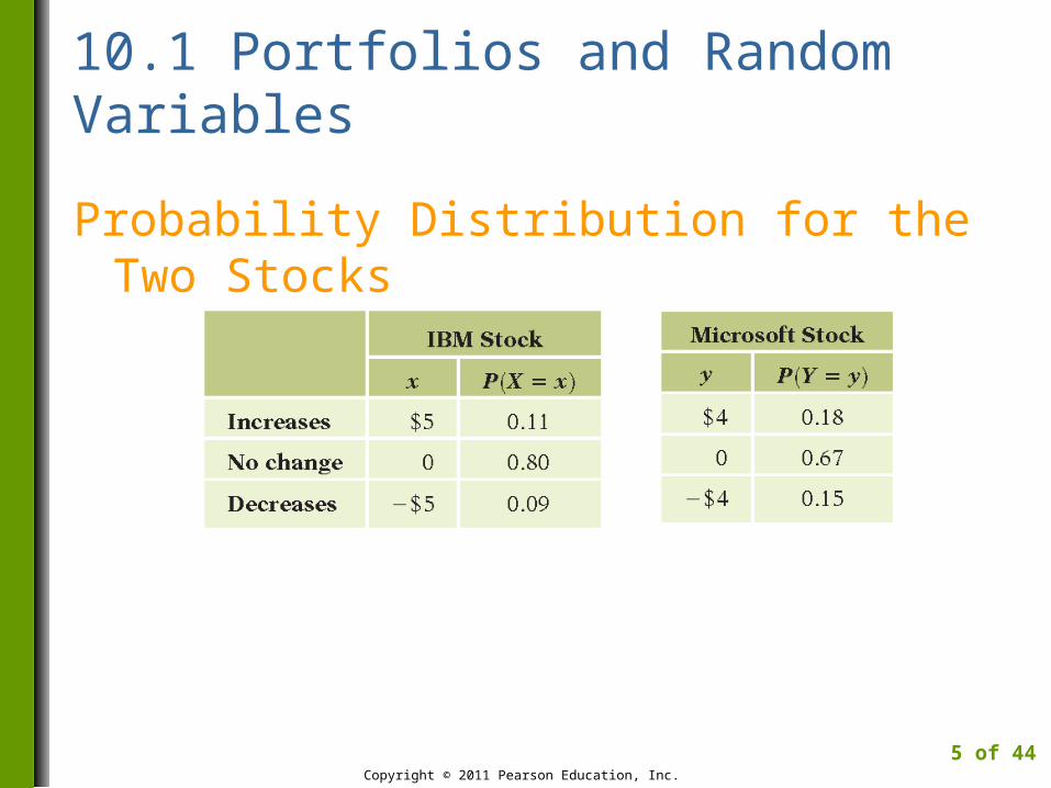
10.1 Portfolios and Random Variables
Probability Distribution for the Two Stocks
Copyright © 2011 Pearson Education, Inc.
5 of 44

10.1 Portfolios and Random Variables
Comparisons and the Sharpe Ratio
The day trader can invest $200 in
Two shares of IBM; Two shares of Microsoft; or One share of each
Copyright © 2011 Pearson Education, Inc.
6 of 44

10.1 Portfolios and Random Variables
Which portfolio should she choose?
Summary of the Two Single Stock Portfolios
Copyright © 2011 Pearson Education, Inc.
7 of 44

10.2 Joint Probability Distribution
Find Sharpe Ratio for Two Stock Portfolio
Combines two different random variables (X and Y) that are not independent
Need joint probability distribution that gives probabilities for events of the form (X = x and Y = y)
Copyright © 2011 Pearson Education, Inc.
8 of 44
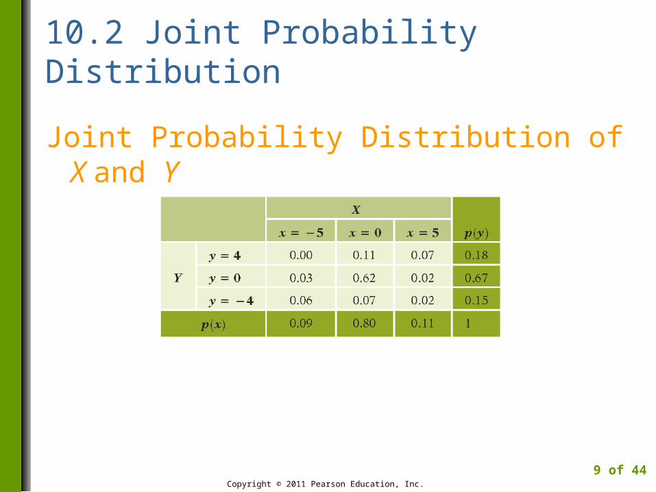
10.2 Joint Probability Distribution
Joint Probability Distribution of X and Y
Copyright © 2011 Pearson Education, Inc.
9 of 44

10.2 Joint Probability Distribution
Independent Random Variables
Two random variables are independent if (and only if) the joint probability distribution is the product of the marginal distributions.
p(x,y) = p(x) p(y) for all x,y
Copyright © 2011 Pearson Education, Inc.
10 of 44
10.2 Joint Probability Distribution
Multiplication Rule
The expected value of a product of independent random variables is the product of their expected values.
E(XY) = E(X)E(Y)
Copyright © 2011 Pearson Education, Inc.
11 of 44

4M Example 10.1: EXCHANGE RATES
Motivation
A firm’s sales in Europe average 10 million € each month. The current exchange rate is 1.40$/€ but it fluctuates. What should this firm expect for the dollar value of European sales next month?
Copyright © 2011 Pearson Education, Inc.
12 of 44

4M Example 10.1: EXCHANGE RATES
Motivation
Fluctuating Exchange Rates
Copyright © 2011 Pearson Education, Inc.
13 of 44

4M Example 10.1: EXCHANGE RATES
Method
Identify three random variables:S = sales next month in €;R = exchange rate next month; and D = value of sales in $.These are related by D = S R. Find E(D).
Copyright © 2011 Pearson Education, Inc.
14 of 44

4M Example 10.1: EXCHANGE RATES
Mechanics
Assume E(R) = 1.40$/€ and independence between S and R.
E(D) = E(R S) = E(S) E(R) = € 10,000,000 1.4 = $14 million
Copyright © 2011 Pearson Education, Inc.
15 of 44

4M Example 10.1: EXCHANGE RATES
Message
European sales for next month convert to $14 million, on average. We assume that sales next month are, on average, the same as in the past for this firm and that sales and exchange rate are independent.
Copyright © 2011 Pearson Education, Inc.
16 of 44
10.2 Joint Probability Distribution
Dependent Random Variables
Joint probability table shows changes in values of IBM and Microsoft (X and Y) are dependent
The dependence between them is positive
Copyright © 2011 Pearson Education, Inc.
17 of 44

10.3 Sums of Random Variables
Addition Rule for Expected Value of a Sum
The expected value of a sum of random variables is the sum of their expected values.
E(X + Y) = E(X) + E(Y)
Copyright © 2011 Pearson Education, Inc.
18 of 44
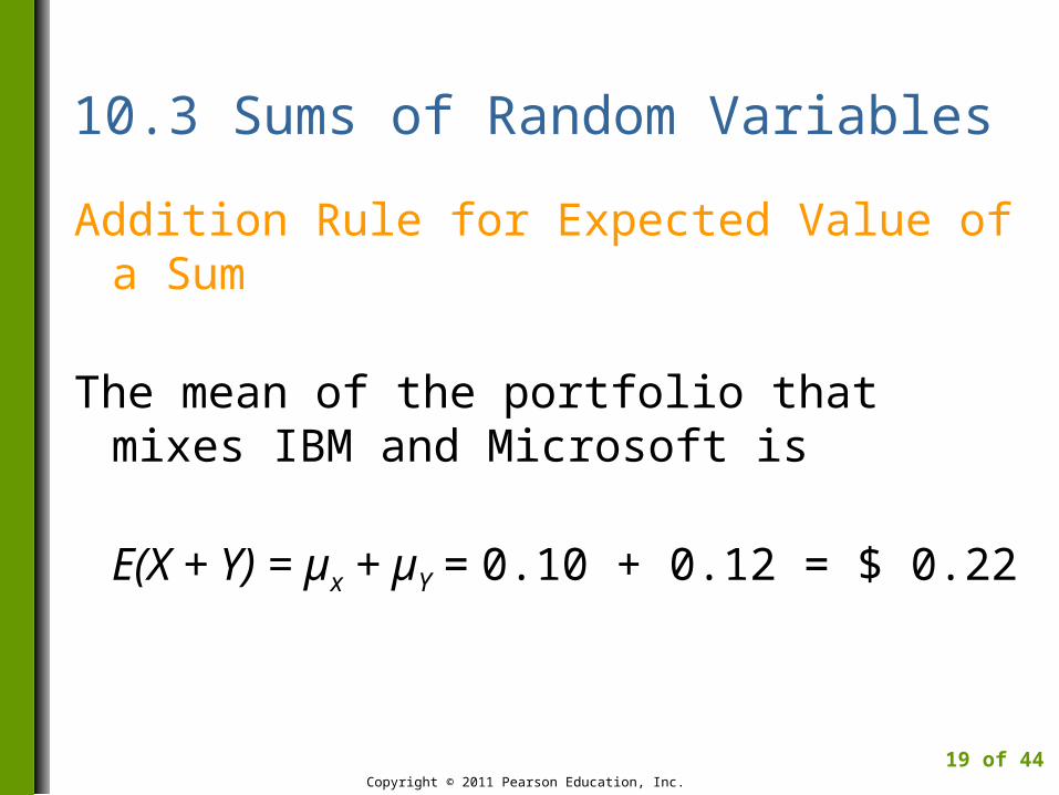
10.3 Sums of Random Variables
Addition Rule for Expected Value of a Sum
The mean of the portfolio that mixes IBM and Microsoft is
E(X + Y) = µx + µY = 0.10 + 0.12 = $ 0.22
Copyright © 2011 Pearson Education, Inc.
19 of 44

10.3 Sums of Random Variables
Variance of a Sum of Random Variables
The variance of a sum of random variables is not necessarily the sum of the variances.
The variance for the portfolio that mixes IBM and Microsoft is larger than the sum:Var(X + Y) = 14.64 $2
Copyright © 2011 Pearson Education, Inc.
20 of 44

10.3 Sums of Random Variables
Sharpe Ratio for Mixed Portfolio
Copyright © 2011 Pearson Education, Inc.
21 of 44
050.064.14
03.022.02
YXVar
rYXS fYX

10.3 Sums of Random Variables
Summary of Sharpe Ratios(Shows Advantage of Diversifying)
Copyright © 2011 Pearson Education, Inc.
22 of 44

10.4 Dependence Between Random Variables
Covariance
The covariance between random variables is the expected value of the product of deviations from the means.
Cov(X,Y) = E((X - µX) (Y - µY))
Copyright © 2011 Pearson Education, Inc.
23 of 44

10.4 Dependence Between Random Variables
Positive Dependence Between X and Y
Copyright © 2011 Pearson Education, Inc.
24 of 44

10.4 Dependence Between Random Variables
Covariance and Sums
The variance of the sum of two random variables is the sum of their variances plus twice their covariance.
Var(X + Y) = Var(X) + Var(Y) + 2Cov(X,Y)
Copyright © 2011 Pearson Education, Inc.
25 of 44

10.4 Dependence Between Random Variables
Using the Addition Rule for Variances
We get the following for the mixed portfolio:
Copyright © 2011 Pearson Education, Inc.
26 of 44
2$64.14
19.2227.599.4
,2
YXCovYVarXVarYXVar

10.4 Dependence Between Random Variables
Correlation
The correlation between two random variables is the covariance divided by the product of standard deviations.
Corr(X,Y) = Cov(X,Y)/σx σY
Copyright © 2011 Pearson Education, Inc.
27 of 44

10.4 Dependence Between Random Variables
Correlation
Denoted by the parameter ρ (“rho”)
Is always between -1 and 1
For the mixed portfolio, ρ = 0.43
Copyright © 2011 Pearson Education, Inc.
28 of 44

10.4 Dependence Between Random Variables
Joint Distribution with ρ = -1
Copyright © 2011 Pearson Education, Inc.
29 of 44

10.4 Dependence Between Random Variables
Joint Distribution with ρ = 1
Copyright © 2011 Pearson Education, Inc.
30 of 44

10.4 Dependence Between Random Variables
Covariance, Correlation and Independence
A correlation of zero does not necessarily imply independence
Independence does imply that the covariance and correlation are zero
Copyright © 2011 Pearson Education, Inc.
31 of 44

10.4 Dependence Between Random Variables
Addition Rule for Variances of Independent Random Variables
The variance of the sum of independent random variables is the sum of their variances.
Var(X + Y) = Var(X) + Var(Y)
Copyright © 2011 Pearson Education, Inc.
32 of 44

10.5 IID Random Variables
Definition
Random variables that are independent of each other and share a common probability distribution are said to be independent and identically distributed.
iid for short
Copyright © 2011 Pearson Education, Inc.
33 of 44

10.5 IID Random Variables
Addition Rule for iid Random Variables
If n random variables (X1, X2, …, Xn) are iid with mean µx and standard deviation σx,
E(X1 + X2 +…+ Xn) = nµx
Var(X1 + X2 +…+ Xn) = nσx2
SD(X1 + X2 +…+ Xn) = σx
Copyright © 2011 Pearson Education, Inc.
34 of 44
n

10.5 IID Random Variables
IID DataStrong link between iid random variables and data
with no pattern (e.g., IBM stock value changes)
Copyright © 2011 Pearson Education, Inc.
35 of 44
10.6 Weighted Sums
Addition Rule for Weighted Sums
The expected value of a weighted sum of random variables is the weighted sum of the expected values.
E(aX + bY + c) = aE(X) + bE(Y) + c
Copyright © 2011 Pearson Education, Inc.
36 of 44

10.6 Weighted Sums
Addition Rule for Weighted Sums
The variance of a weighted sum of random variables is
Var(aX + bY + c) = a2Var(X) + b2Var(Y) + 2abCov(X,Y)
Copyright © 2011 Pearson Education, Inc.
37 of 44
4M Example 10.2: CONSTRUCTION ESTIMATES
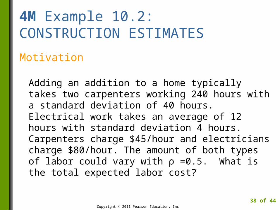
Motivation
Adding an addition to a home typically takes two carpenters working 240 hours with a standard deviation of 40 hours. Electrical work takes an average of 12 hours with standard deviation 4 hours. Carpenters charge $45/hour and electricians charge $80/hour. The amount of both types of labor could vary with ρ =0.5. What is the total expected labor cost?
Copyright © 2011 Pearson Education, Inc.
38 of 44

4M Example 10.2: CONSTRUCTION ESTIMATES
Method
Identify three random variables:X = number of carpentry hours;Y = number of electrician hours; and T = total costs ($).These are related by T = 45X + 80Y.
Copyright © 2011 Pearson Education, Inc.
39 of 44

4M Example 10.2: CONSTRUCTION ESTIMATES
Mechanics: Find E(T) Using Addition Rule for Weighted Sums
Copyright © 2011 Pearson Education, Inc.
40 of 44
760,11$
12802404580458045
YEXEYXETE

4M Example 10.2: CONSTRUCTION ESTIMATES
Mechanics: Find Var(T) Using the Addition Rule for Weighted Sums
Copyright © 2011 Pearson Education, Inc.
41 of 44
804405.0, YXYXCov
400,918,3
000,576400,102000,240,3
80804524804045
,80452804580452222
22
YXCovYVarXVarYXVarTVar

4M Example 10.2: CONSTRUCTION ESTIMATES
Message
The expected total cost for labor is around $12,000 with a standard deviation of about $2,000.
Copyright © 2011 Pearson Education, Inc.
42 of 44

Best Practices
Consider the possibility of dependence.
Only add variances for random variables that are uncorrelated.
Use several random variables to capture different features of a problem.
Use new symbols for each random variable.
Copyright © 2011 Pearson Education, Inc.
43 of 44

Pitfalls
Do not think that uncorrelated random variables are independent.
Don’t forget the covariance when finding the variance of a sum.
Never add standard deviations of random variables.
Don’t mistake Var(X – Y) for Var(X) – Var(Y).
Copyright © 2011 Pearson Education, Inc.
44 of 44