convergence dynamics in the andean community - … dynamics in the andean community josé pineda...

Convergence Dynamics in the Andean Community

José Pineda

Corporación Andina de Fomento

Universidad Central de Venezuela

April, 2006

Abstract

In this paper, we present some evidence on convergence dynamics in the Andean Community. Our results indicate that there has been a reduction on income disparities across countries in the Andean Community. However, at the regional level, our results show that inequality within countries is not only important, it represents around 75% of regional inequality in the Andean Community, but has also been increasing over time. We also decompose the total change in inequality in order to analyze the contribution of income and population changes. We find that for the Andean Community inequality changes are mostly produced by income changes, which explain 96% of total changes. We also explore the existence of unconditional beta convergence in the Andean Community. In general, we find evidence of convergence among Andean countries and regions within each country, and this convergence is faster when we control for country characteristics that determine each country steady-state level. Also, our results indicate that there exist regional factors preventing poor regions to converge faster than richer regions. We also report results about income distribution dynamics indicating that the distribution became less dense in the tails and thinner in the middle. However, although regions are converging to the middle, this is not explained by a greater growth of poorer regions but mainly for the decline experienced by richer regions; in particular the decline experienced by Venezuelan regions.

I wish to thank Juan Blyde whose research for MERCOSUR serves as a motivation of this paper and as a point of comparison for many of my results. I want to thank Osvaldo Nina and Paul Carrillo for their comments at CAF’s seminar. I also want to thank the comments and suggestions made by Daniel Ortega, Rodolfo Méndez, Adriana Arreaza, Osmel Manzano, Alejandro Puente and the rest of participants at IESA’s Seminar of Public Policy; and Ricardo Isea, Mariana Penzini and Federico Ortega for excellent research assistance. All the errors are responsibility of the author. Email: [email protected]

1. Introduction

The analysis of regional disparities is of special interest for countries that are

involved in a process of economic integration. This is particular true, given the fact that

traditional trade theory states that, for a given distribution of endowments of natural

resources, factors of production, infrastructure or technology (which provides the incentives

for countries to trade), the removal of obstacles to the movement of goods and/or factors

would cause convergence of factor returns and living standards. This seems to be the case

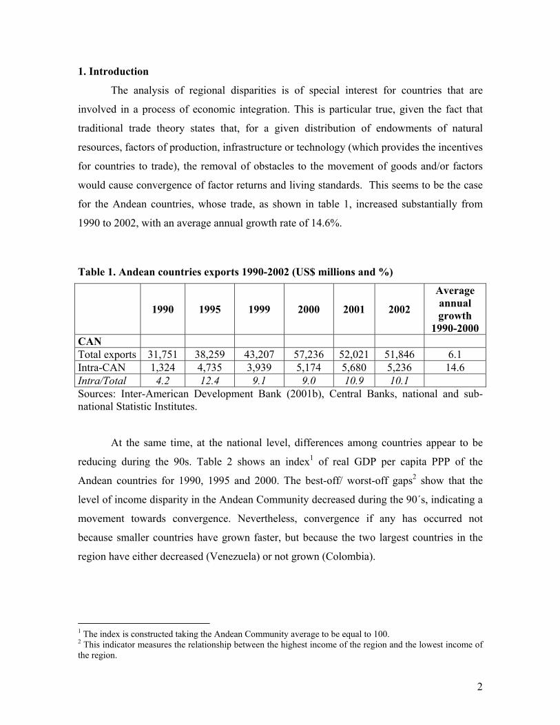
for the Andean countries, whose trade, as shown in table 1, increased substantially from

1990 to 2002, with an average annual growth rate of 14.6%.

Table 1. Andean countries exports 1990-2002 (US$ millions and %)

1990 1995 1999 2000 2001 2002

Average annual growth

1990-2000 CAN Total exports 31,751 38,259 43,207 57,236 52,021 51,846 6.1 Intra-CAN 1,324 4,735 3,939 5,174 5,680 5,236 14.6 Intra/Total 4.2 12.4 9.1 9.0 10.9 10.1 Sources: Inter-American Development Bank (2001b), Central Banks, national and sub-national Statistic Institutes.

At the same time, at the national level, differences among countries appear to be

reducing during the 90s. Table 2 shows an index1 of real GDP per capita PPP of the

Andean countries for 1990, 1995 and 2000. The best-off/ worst-off gaps2 show that the

level of income disparity in the Andean Community decreased during the 90´s, indicating a

movement towards convergence. Nevertheless, convergence if any has occurred not

because smaller countries have grown faster, but because the two largest countries in the

region have either decreased (Venezuela) or not grown (Colombia).

1 The index is constructed taking the Andean Community average to be equal to 100. 2 This indicator measures the relationship between the highest income of the region and the lowest income of the region.

2

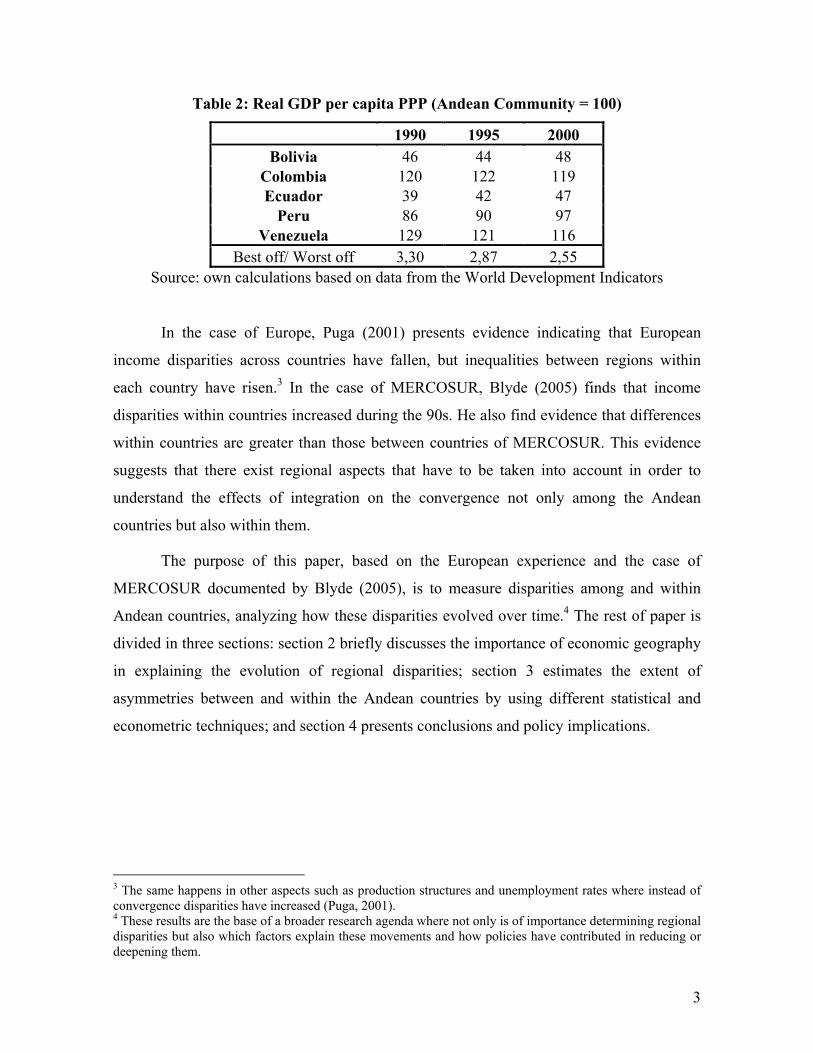
Table 2: Real GDP per capita PPP (Andean Community = 100)

1990 1995 2000 Bolivia 46 44 48

Colombia 120 122 119 Ecuador 39 42 47

Peru 86 90 97 Venezuela 129 121 116

Best off/ Worst off 3,30 2,87 2,55 Source: own calculations based on data from the World Development Indicators

In the case of Europe, Puga (2001) presents evidence indicating that European

income disparities across countries have fallen, but inequalities between regions within

each country have risen.3 In the case of MERCOSUR, Blyde (2005) finds that income

disparities within countries increased during the 90s. He also find evidence that differences

within countries are greater than those between countries of MERCOSUR. This evidence

suggests that there exist regional aspects that have to be taken into account in order to

understand the effects of integration on the convergence not only among the Andean

countries but also within them.

The purpose of this paper, based on the European experience and the case of

MERCOSUR documented by Blyde (2005), is to measure disparities among and within

Andean countries, analyzing how these disparities evolved over time.4 The rest of paper is

divided in three sections: section 2 briefly discusses the importance of economic geography

in explaining the evolution of regional disparities; section 3 estimates the extent of

asymmetries between and within the Andean countries by using different statistical and

econometric techniques; and section 4 presents conclusions and policy implications.

3 The same happens in other aspects such as production structures and unemployment rates where instead of convergence disparities have increased (Puga, 2001). 4 These results are the base of a broader research agenda where not only is of importance determining regional disparities but also which factors explain these movements and how policies have contributed in reducing or deepening them.

3

2. Economic geography and regional disparities5

The “new economic geography” could be useful to explain trends on countries’ and

regions’ disparities. It brings together the forces that affect the evolution of regional

differences over time (convergence and divergence forces). The main intuition of this

literature can be explained through a Core-Periphery model that highlights the interaction

between agglomeration and dispersion forces.

The agglomeration forces mainly depend on what is called “market access effects”,

which describe the incentive of firms to locate their production in big markets and export to

small markets. Also, they are influenced by the “cost of living effect”, which implies that

goods would be cheaper in regions were more industrial firms are located. Finally, they

could be enhanced by what is known as “circular causality”, when both market access

effect and cost of living effect reinforce each other. For example, changes in market size

could induce firms to relocate to the larger market, which would be reinforced by the

attractiveness of a higher wage in the larger market.

Alternatively, the diverging forces are related, firstly, to what are known as “market

crowding effects”, which reflect the tendency of firms and/or workers to locate in regions

with relatively few competitors. For example, the shifting of firms towards the larger

market increases competition for workers, which lowers wages, so workers will move to

the smaller market in search of higher wages. Secondly, we have the “congestion effect”,

which consist in an important increase in factor’ costs (in particular factors with low

mobility) due to a higher firms concentration, and, as a result, firms will be looking for new

geographic locations.

The way throughout agglomeration and dispersion forces affect firm’s location is

influenced by the level of trade costs. Models help explain why regions without different

comparative advantages can develop different production structures on the basis of their

different market accesses. Krugman and Venables (1990) formalized the location

implications of a model of trade with increasing returns and imperfect competition. They

5 This section is based on Puga (2001) and Manuscript for Economic Geography and Public Policy © 2002 Baldwin, Forslid, Martin, Ottaviano & Robert-Nicoud.

4

analyzed a model with two regions with the same relative endowments:6 a large core region

and a small peripheral region. Two sectors, a competitive one that produced homogeneous

tradable commodities under constant returns to scale; and an imperfectly competitive sector

producing manufactures under increasing returns to scale. They found that for finite

positive trade costs, the core’s share of industry is larger than its share of endowments, and

it is therefore a net exporter of manufactures.7 This effect is known as the market access

effect.

They also reported an ambiguous effect of economic integration and reductions in

transport costs on the relative attractiveness of core and peripheral regions. On the one

hand, economic integration increases the share of sales that each firm makes in the other

region, weakening the effect of more local competitors on each firm’s market share. Yet

increasing returns imply that the larger sales of firms producing in the core give them

higher profits. If more firms enter in response to those profits, the size of industry in the

core rises above its share of world endowments.

On the other hand, if trade is almost free, the movement from one market to another

will have a small impact on firm’s revenues, and wages differences will tend to disappear,

inducing the region’s share of industry to go back to its overall share of endowments. The

analysis of these forces indicates the existence of a trade-off between the economic

advantages of the clustering of activity and the inequalities that it may bring.

For Latin America there are few evidence regarding the behavior of such forces

after the trade liberalization. For the Mexican case, Hanson (1998) shows that trade

liberalization generated a reallocation of industrial employment towards the north zone,

near the border with the United States. In addition, for the case of Argentina, Sanguinetti

and Volpe (2005) show that there are important agglomeration forces in the industrial

employment in Argentina, which have led to a strong concentration in few regions (only

Buenos Aires concentrate 44% of the total industrial employment). However, evidence also

shows that although there haven’t had substantial changes in this pattern, Argentina

6 This implies that both regions have the same comparative advantages, and only economic geography effects will be in place. 7 Notice that in this type of model similar regions can end up with different production structures and income levels, which is not the case for traditional trade models.

5

experimented a slightly decreasing trend in the concentration of industrial employment

since middle eighties until middle nineties. Besides, authors have documented the central

role of the trade policy on the determination of location patterns of the Argentinean

industrial activities, where tariffs’ reduction have conduced to a special dispersion of the

industries.

The evidence in both cases, Argentina and Mexico, shows that trade openness affect

the relative importance of international markets in comparison to local markets. This

encourage firms to take decisions related to production’s location not only based on the

local market supply, but also in accordance with its exports destination. This have been

particularly reflected in the case of Mexico, whose trend have been towards to a major

concentration of its production activities due to its strong exports concentration, principally

to the United States market.

3. Disparities of Incomes in the Andean countries

In this section, we measure income disparities in the Andean countries through the

use of a battery of inequality indexes. 8 We begin by measuring disparities across national

incomes, and later analyze income disparities across regions within countries and explain

how the two levels of aggregation are related.

Here we follow the relatively recent use that economists have given, in regional and

national contexts, to some inequality indexes that have been extensively employed in the

literature of inequality measurement with household data (see for example, Duro (2001),

Puga (2001), and Blyde (2005)).

In this section, we use three inequality measures to analyze income disparity in the

Andean Community:9 the sigma-dispersion,10 the Gini coefficient11 and the Theil

population-weighted index.12

8 In section 3.4, we will discuss what is called in the literature of economic growth “Beta Unconditional Convergence”. 9 In this paper, we present some of the most common inequality measures used in the literature in order to make our work as comparable as possible. However, not all the inequality measures that are used behave in the same fashion. This is why the inequality measurement literature has used some axioms for identifying “satisfactory measures” of inequality. The axioms considered are: The Pigou-Dalton Transfer, income scale independence, principle of population, anonymity and decomposability (see Poverty Net at the World Bank web page). 10 The sigma-dispersion measure is simply the (non-weighted) standard deviation of logarithms of incomes.

6

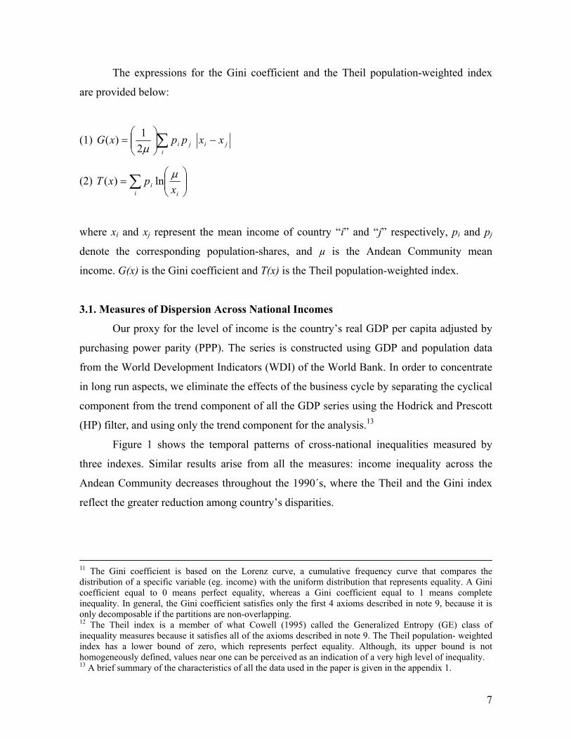
The expressions for the Gini coefficient and the Theil population-weighted index

are provided below:

(1) ∑ −

=

ijiji xxppx

µ21)G(

(2)

= ∑

iii x

px µln)(T

where xi and xj represent the mean income of country “i” and “j” respectively, pi and pj

denote the corresponding population-shares, and µ is the Andean Community mean

income. G(x) is the Gini coefficient and T(x) is the Theil population-weighted index.

3.1. Measures of Dispersion Across National Incomes

Our proxy for the level of income is the country’s real GDP per capita adjusted by

purchasing power parity (PPP). The series is constructed using GDP and population data

from the World Development Indicators (WDI) of the World Bank. In order to concentrate

in long run aspects, we eliminate the effects of the business cycle by separating the cyclical

component from the trend component of all the GDP series using the Hodrick and Prescott

(HP) filter, and using only the trend component for the analysis.13

Figure 1 shows the temporal patterns of cross-national inequalities measured by

three indexes. Similar results arise from all the measures: income inequality across the

Andean Community decreases throughout the 1990´s, where the Theil and the Gini index

reflect the greater reduction among country’s disparities.

11 The Gini coefficient is based on the Lorenz curve, a cumulative frequency curve that compares the distribution of a specific variable (eg. income) with the uniform distribution that represents equality. A Gini coefficient equal to 0 means perfect equality, whereas a Gini coefficient equal to 1 means complete inequality. In general, the Gini coefficient satisfies only the first 4 axioms described in note 9, because it is only decomposable if the partitions are non-overlapping. 12 The Theil index is a member of what Cowell (1995) called the Generalized Entropy (GE) class of inequality measures because it satisfies all of the axioms described in note 9. The Theil population- weighted index has a lower bound of zero, which represents perfect equality. Although, its upper bound is not homogeneously defined, values near one can be perceived as an indication of a very high level of inequality. 13 A brief summary of the characteristics of all the data used in the paper is given in the appendix 1.

7

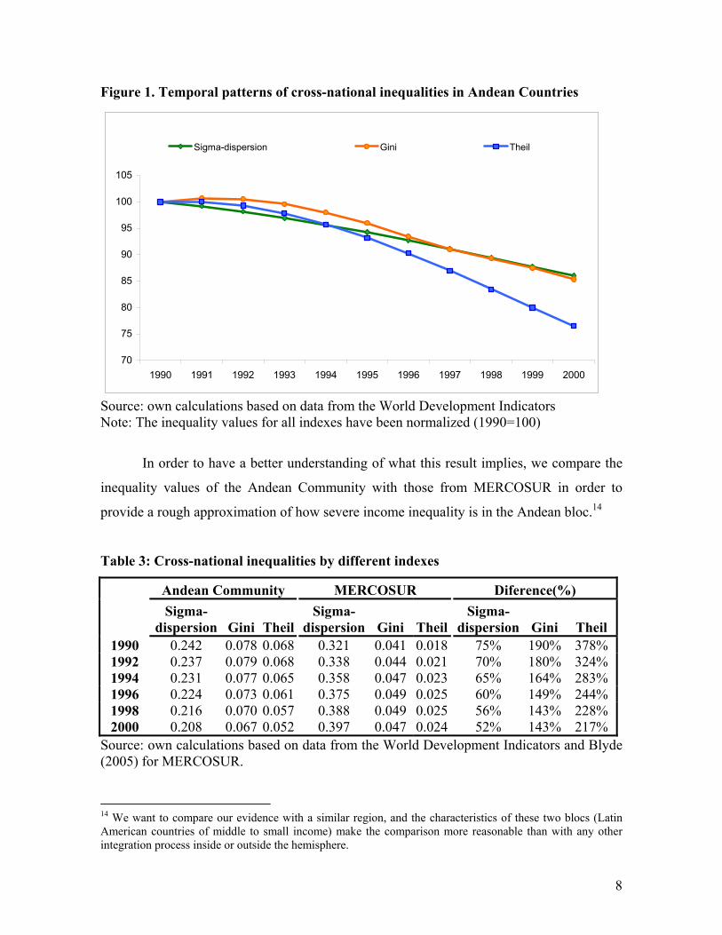
Figure 1. Temporal patterns of cross-national inequalities in Andean Countries

70

75

80

85

90

95

100

105

1990 1991 1992 1993 1994 1995 1996 1997 1998 1999 2000

Sigma-dispersion Gini Theil

Source: own calculations based on data from the World Development Indicators Note: The inequality values for all indexes have been normalized (1990=100)

In order to have a better understanding of what this result implies, we compare the

inequality values of the Andean Community with those from MERCOSUR in order to

provide a rough approximation of how severe income inequality is in the Andean bloc.14

Table 3: Cross-national inequalities by different indexes

Andean Community MERCOSUR Diference(%)

Sigma-

dispersion Gini TheilSigma-


dispersion Gini Theil 1990 0.242 0.078 0.068 0.321 0.041 0.018 75% 190% 378% 1992 0.237 0.079 0.068 0.338 0.044 0.021 70% 180% 324% 1994 0.231 0.077 0.065 0.358 0.047 0.023 65% 164% 283% 1996 0.224 0.073 0.061 0.375 0.049 0.025 60% 149% 244% 1998 0.216 0.070 0.057 0.388 0.049 0.025 56% 143% 228% 2000 0.208 0.067 0.052 0.397 0.047 0.024 52% 143% 217%

Source: own calculations based on data from the World Development Indicators and Blyde (2005) for MERCOSUR.

14 We want to compare our evidence with a similar region, and the characteristics of these two blocs (Latin American countries of middle to small income) make the comparison more reasonable than with any other integration process inside or outside the hemisphere.

8

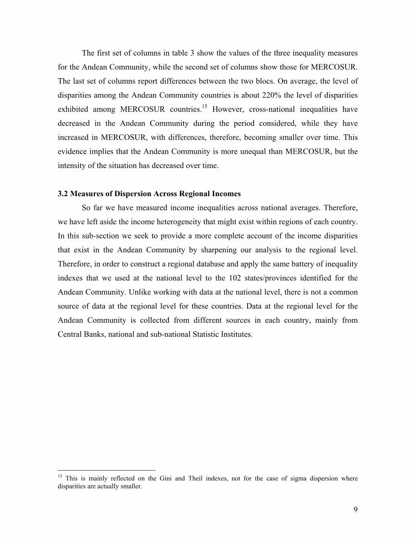
The first set of columns in table 3 show the values of the three inequality measures

for the Andean Community, while the second set of columns show those for MERCOSUR.

The last set of columns report differences between the two blocs. On average, the level of

disparities among the Andean Community countries is about 220% the level of disparities

exhibited among MERCOSUR countries.15 However, cross-national inequalities have

decreased in the Andean Community during the period considered, while they have

increased in MERCOSUR, with differences, therefore, becoming smaller over time. This

evidence implies that the Andean Community is more unequal than MERCOSUR, but the

intensity of the situation has decreased over time.

3.2 Measures of Dispersion Across Regional Incomes

So far we have measured income inequalities across national averages. Therefore,

we have left aside the income heterogeneity that might exist within regions of each country.

In this sub-section we seek to provide a more complete account of the income disparities

that exist in the Andean Community by sharpening our analysis to the regional level.

Therefore, in order to construct a regional database and apply the same battery of inequality

indexes that we used at the national level to the 102 states/provinces identified for the

Andean Community. Unlike working with data at the national level, there is not a common

source of data at the regional level for these countries. Data at the regional level for the

Andean Community is collected from different sources in each country, mainly from

Central Banks, national and sub-national Statistic Institutes.

15 This is mainly reflected on the Gini and Theil indexes, not for the case of sigma dispersion where disparities are actually smaller.

9

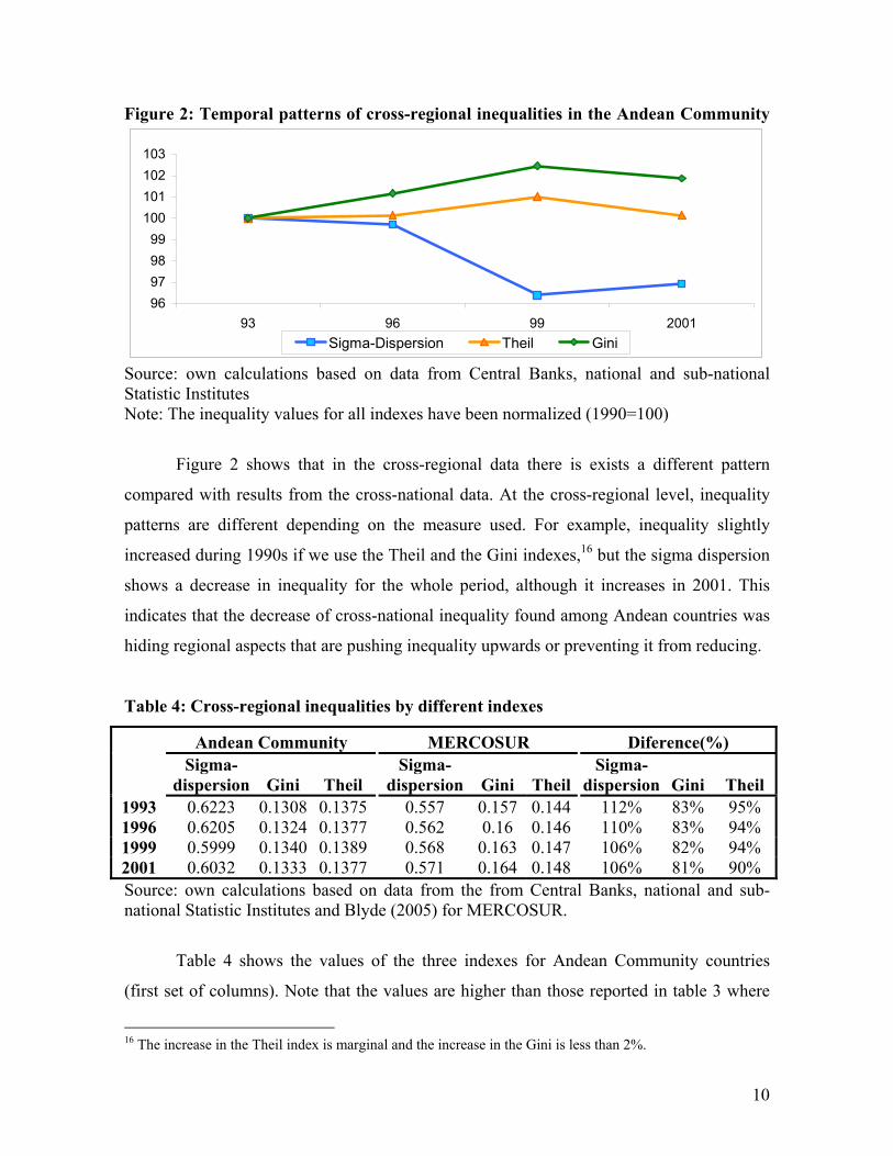
Figure 2: Temporal patterns of cross-regional inequalities in the Andean Community

96979899100101102103

93 96 99 2001Sigma-Dispersion Theil Gini

Source: own calculations based on data from Central Banks, national and sub-national Statistic Institutes Note: The inequality values for all indexes have been normalized (1990=100)

Figure 2 shows that in the cross-regional data there is exists a different pattern

compared with results from the cross-national data. At the cross-regional level, inequality

patterns are different depending on the measure used. For example, inequality slightly

increased during 1990s if we use the Theil and the Gini indexes,16 but the sigma dispersion

shows a decrease in inequality for the whole period, although it increases in 2001. This

indicates that the decrease of cross-national inequality found among Andean countries was

hiding regional aspects that are pushing inequality upwards or preventing it from reducing.

Table 4: Cross-regional inequalities by different indexes

Andean Community MERCOSUR Diference(%)

Sigma-

dispersion Gini Theil Sigma-


dispersion Gini Theil 1993 0.6223 0.1308 0.1375 0.557 0.157 0.144 112% 83% 95% 1996 0.6205 0.1324 0.1377 0.562 0.16 0.146 110% 83% 94% 1999 0.5999 0.1340 0.1389 0.568 0.163 0.147 106% 82% 94% 2001 0.6032 0.1333 0.1377 0.571 0.164 0.148 106% 81% 90% Source: own calculations based on data from the from Central Banks, national and sub-national Statistic Institutes and Blyde (2005) for MERCOSUR.

Table 4 shows the values of the three indexes for Andean Community countries

(first set of columns). Note that the values are higher than those reported in table 3 where

16 The increase in the Theil index is marginal and the increase in the Gini is less than 2%.

10

we only measure inequalities between countries. Therefore, the heterogeneity within

countries is an important part of overall inequality in Andean Community countries. In the

next section, we will tackle this point by decomposing the overall inequality into two

components: inequality between countries and within countries.

We also compare inequality levels in the Andean Community with those in

MERCOSUR. The second set of columns in table 4 shows the results for MERCOSUR,

while the last set of columns report the differences between the two blocs. Same as before,

the differences between the two blocs have become smaller over time. But now, at the

regional level, not all inequality indexes are larger than those of MERCOSUR. In fact, both

Theil and Gini are smaller for Andean Community countries than for MERCOSUR

countries. On average, the level of regional disparities in the Andean Community is close to

95% the exhibited regional disparities in MERCOSUR. Then, we can say by the evidence

presented in table 4 that regional income inequality in the Andean Community is

significant, although not much higher than that in MERCOSUR, and the differences

between the two blocs have been declining over time.

3.3. Inequality Decomposition: Within and Between Groups

Results from the previous sections suggest differences in the contribution of income

inequality at the national and regional levels. In this section we explore the ability of the

Theil index of being able to be partitioned into disjoint subgroups in order to decompose

the overall degree of regional inequality (reflected by T(x)) into two different components:

the within-country inequality factor and the between-country inequality factor. The first

component is computed as a weighted mean of intra-country inequality indexes. The

second component reflects the inequality that would emerge if there were only differences

were among country means. The decomposition of the Theil index, T(x), may be written as

follows:

(3) T ( )g

G

ggg

G

ggBW xpxTpxTxTx /ln)()()()(

11µ∑∑

==

+=+=

where TW (x) is the aggregate within-country inequality component; TB(x) is the aggregate

between-country inequality component; pg is the relative population of country “g”; T(x)g

11

denotes the internal inequality present in country “g”, and xg represents the national mean

income in country “g”.

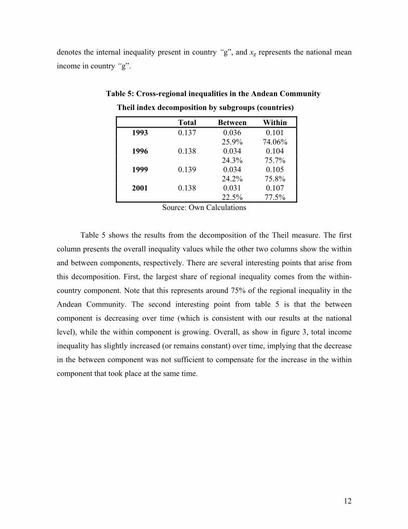
Table 5: Cross-regional inequalities in the Andean Community

Theil index decomposition by subgroups (countries)

Total Between Within 1993 0.137 0.036 0.101

25.9% 74.06% 1996 0.138 0.034 0.104

24.3% 75.7% 1999 0.139 0.034 0.105

24.2% 75.8% 2001 0.138 0.031 0.107

22.5% 77.5% Source: Own Calculations

Table 5 shows the results from the decomposition of the Theil measure. The first

column presents the overall inequality values while the other two columns show the within

and between components, respectively. There are several interesting points that arise from

this decomposition. First, the largest share of regional inequality comes from the within-

country component. Note that this represents around 75% of the regional inequality in the

Andean Community. The second interesting point from table 5 is that the between

component is decreasing over time (which is consistent with our results at the national

level), while the within component is growing. Overall, as show in figure 3, total income

inequality has slightly increased (or remains constant) over time, implying that the decrease

in the between component was not sufficient to compensate for the increase in the within

component that took place at the same time.

12

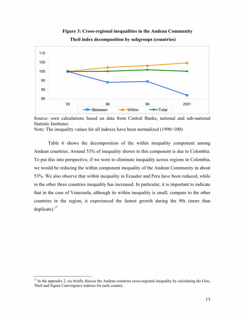
Figure 3: Cross-regional inequalities in the Andean Community

Theil index decomposition by subgroups (countries)

85

90

95

100

105

110

93 96 99 2001Between Within Total

Source: own calculations based on data from Central Banks, national and sub-national Statistic Institutes Note: The inequality values for all indexes have been normalized (1990=100)

Table 6 shows the decomposition of the within inequality component among

Andean countries. Around 53% of inequality shown in this component is due to Colombia.

To put this into perspective, if we were to eliminate inequality across regions in Colombia,

we would be reducing the within component inequality of the Andean Community in about

53%. We also observe that within inequality in Ecuador and Peru have been reduced, while

in the other three countries inequality has increased. In particular, it is important to indicate

that in the case of Venezuela, although its within inequality is small, compare to the other

countries in the region, it experienced the fastest growth during the 90s (more than

duplicate).17

17 In the appendix 2, we briefly discuss the Andean countries cross-regional inequality by calculating the Gini, Theil and Sigma Convergence indexes for each country.

13

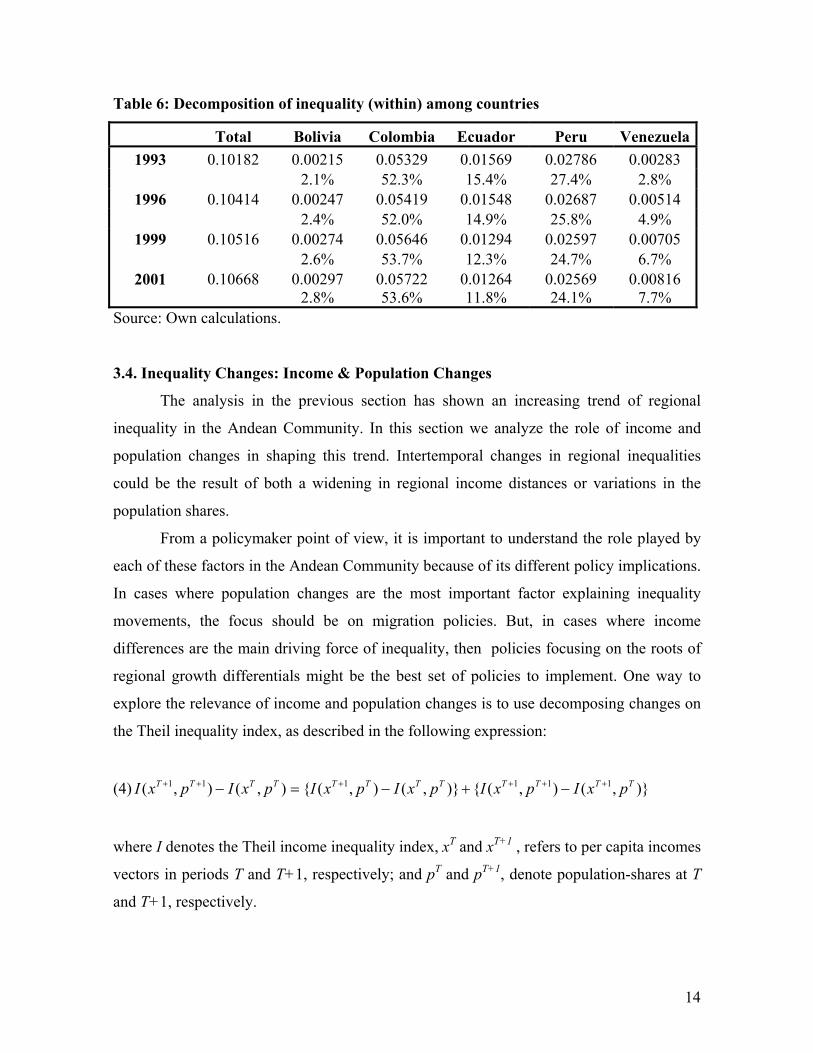
Table 6: Decomposition of inequality (within) among countries

Total Bolivia Colombia Ecuador Peru Venezuela1993 0.10182 0.00215 0.05329 0.01569 0.02786 0.00283

2.1% 52.3% 15.4% 27.4% 2.8% 1996 0.10414 0.00247 0.05419 0.01548 0.02687 0.00514

2.4% 52.0% 14.9% 25.8% 4.9% 1999 0.10516 0.00274 0.05646 0.01294 0.02597 0.00705

2.6% 53.7% 12.3% 24.7% 6.7% 2001 0.10668 0.00297 0.05722 0.01264 0.02569 0.00816

2.8% 53.6% 11.8% 24.1% 7.7% Source: Own calculations.

3.4. Inequality Changes: Income & Population Changes

The analysis in the previous section has shown an increasing trend of regional

inequality in the Andean Community. In this section we analyze the role of income and

population changes in shaping this trend. Intertemporal changes in regional inequalities

could be the result of both a widening in regional income distances or variations in the

population shares.

From a policymaker point of view, it is important to understand the role played by

each of these factors in the Andean Community because of its different policy implications.

In cases where population changes are the most important factor explaining inequality

movements, the focus should be on migration policies. But, in cases where income

differences are the main driving force of inequality, then policies focusing on the roots of

regional growth differentials might be the best set of policies to implement. One way to

explore the relevance of income and population changes is to use decomposing changes on

the Theil inequality index, as described in the following expression:

(4) )},(),({)},(),({),(),( 111111 TTTTTTTTTTTT pxIpxIpxIpxIpxIpxI ++++++ −+−=−

where I denotes the Theil income inequality index, xT and xT+1 , refers to per capita incomes

vectors in periods T and T+1, respectively; and pT and pT+1, denote population-shares at T

and T+1, respectively.

14

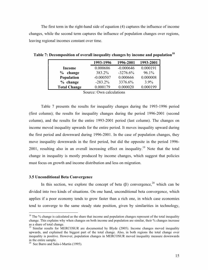
The first term in the right-hand side of equation (4) captures the influence of income

changes, while the second term captures the influence of population changes over regions,

leaving regional incomes constant over time.

Table 7: Decomposition of overall inequality changes by income and population18

1993-1996 1996-2001 1993-2001 Income 0.000686 -0.000646 0.000191

% change 383.2% -3276.6% 96.1% Population -0.000507 0.000666 0.000008 % change -283.2% 3376.6% 3.9%

Total Change 0.000179 0.000020 0.000199 Source: Own calculations

Table 7 presents the results for inequality changes during the 1993-1996 period

(first column); the results for inequality changes during the period 1996-2001 (second

column), and the results for the entire 1993-2001 period (last column). The changes on

income moved inequality upwards for the entire period. It moves inequality upward during

the first period and downward during 1996-2001. In the case of population changes, they

move inequality downwards in the first period, but did the opposite in the period 1996-

2001, resulting also in an overall increasing effect on inequality.19 Note that the total

change in inequality is mostly produced by income changes, which suggest that policies

must focus on growth and income distribution and less on migration.

3.5 Unconditional Beta Convergence

In this section, we explore the concept of beta (β) convergence,20 which can be

divided into two kinds of situations. On one hand, unconditional beta convergence, which

applies if a poor economy tends to grow faster than a rich one, in which case economies

tend to converge to the same steady state position, given by similarities in technology, 18 The % change is calculated as the share that income and population changes represent of the total inequality change. This explains why when changes on both income and population are similar, their % changes increase as a share of total change. 19 Similar results for MERCOSUR are documented by Blyde (2005). Income changes moved inequality upwards, and explained the biggest part of the total change. Also, in both regions the total change over inequality is positive. However, population changes in MERCOSUR moved inequality measure downwards in the entire sample. 20 See Barro and Sala-i-Martin (1995).

15

preferences, and institutions.21 On the other hand, conditional beta convergence, which

implies that an economy that starts out proportionality further below its own steady state

tends to grow faster. That is, if the economies have significant differences in parameters

like technology, preferences and institutions, they will have important differences in their

steady state positions, and the growth product rate of each economy will be inversely

related with the distance from its steady-state position.22 23

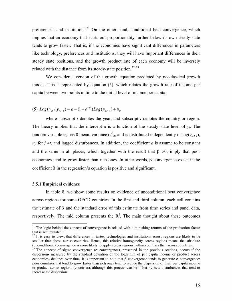
We consider a version of the growth equation predicted by neoclassical growth

model. This is represented by equation (5), which relates the growth rate of income per

capita between two points in time to the initial level of income per capita:

(5) ittitiit uyLogeayyLog +−−= −−

− )()1()/( 1,1,β

where subscript t denotes the year, and subscript i denotes the country or region.

The theory implies that the intercept a is a function of the steady–state level of yi. The

random variable uit has 0 mean, variance σ2ut, and is distributed independently of log(yi, t-1),

ujt for j ≠t, and lagged disturbances. In addition, the coefficient a is assume to be constant

and the same in all places, which together with the result that β >0, imply that poor

economies tend to grow faster than rich ones. In other words, β convergence exists if the

coefficient β in the regression’s equation is positive and significant.

3.5.1 Empirical evidence

In table 8, we show some results on evidence of unconditional beta convergence

across regions for some OECD countries. In the first and third column, each cell contains

the estimate of β and the standard error of this estimate from time series and panel data,

respectively. The mid column presents the R2. The main thought about these outcomes 21 The logic behind the concept of convergence is related with diminishing returns of the production factor that is accumulated. 22 It is easy to view, that differences in tastes, technologies and institutions across regions are likely to be smaller than those across countries. Hence, this relative homogeneity across regions means that absolute (unconditional) convergence is more likely to apply across regions within countries than across countries. 23 The concept of sigma convergence (σ convergence), presented in the previous sections, occurs if the dispersion- measured by the standard deviation of the logarithm of per capita income or product across economies- declines over time. It is important to note that β convergence tends to generate σ convergence: poor countries that tend to grow faster than rich ones tend to reduce the dispersion of their per capita income or product across regions (countries), although this process can be offset by new disturbances that tend to increase the dispersion.

16

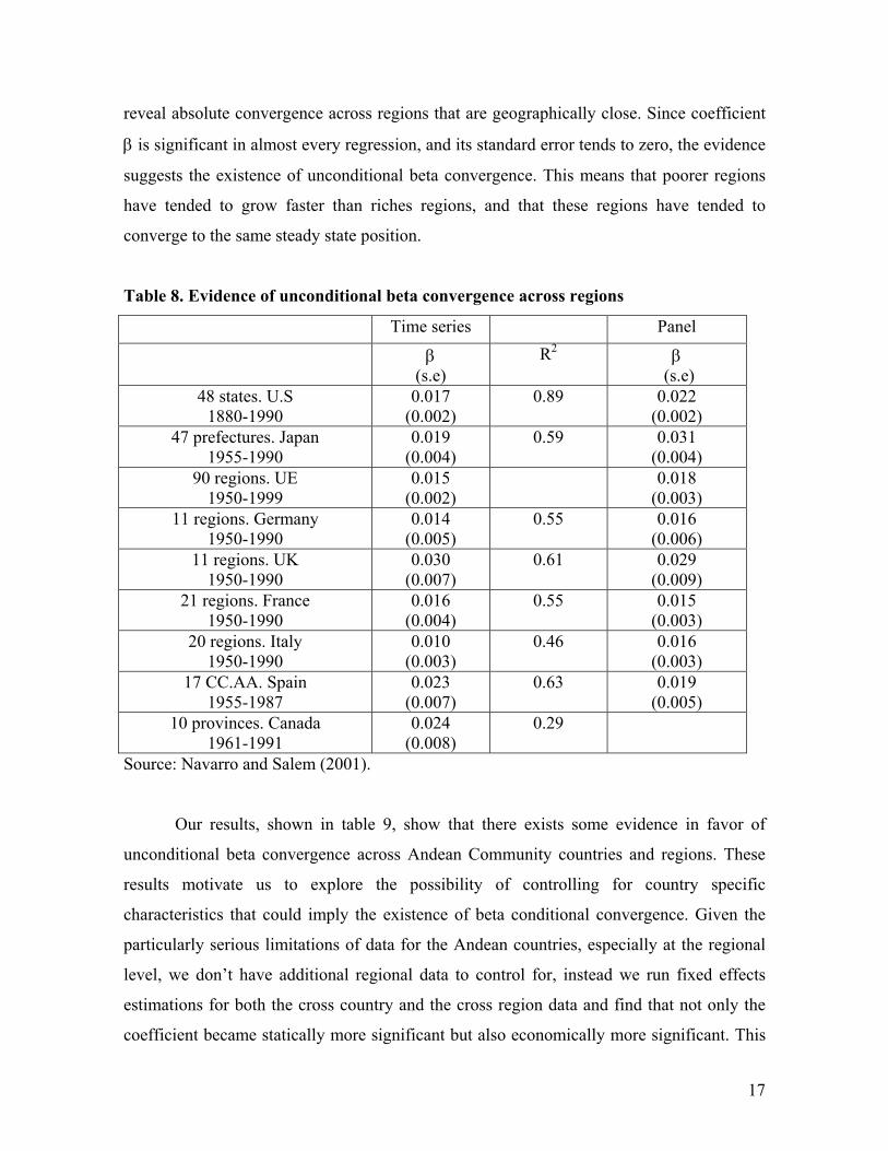
reveal absolute convergence across regions that are geographically close. Since coefficient

β is significant in almost every regression, and its standard error tends to zero, the evidence

suggests the existence of unconditional beta convergence. This means that poorer regions

have tended to grow faster than riches regions, and that these regions have tended to

converge to the same steady state position.

Table 8. Evidence of unconditional beta convergence across regions

Time series Panel β

(s.e) R2 β

(s.e) 48 states. U.S

1880-1990 0.017

(0.002) 0.89 0.022

(0.002) 47 prefectures. Japan

1955-1990 0.019

(0.004) 0.59 0.031

(0.004) 90 regions. UE

1950-1999 0.015

(0.002) 0.018

(0.003) 11 regions. Germany

1950-1990 0.014

(0.005) 0.55 0.016

(0.006) 11 regions. UK

1950-1990 0.030

(0.007) 0.61 0.029

(0.009) 21 regions. France

1950-1990 0.016

(0.004) 0.55 0.015

(0.003) 20 regions. Italy

1950-1990 0.010

(0.003) 0.46 0.016

(0.003) 17 CC.AA. Spain

1955-1987 0.023

(0.007) 0.63 0.019

(0.005) 10 provinces. Canada

1961-1991 0.024

(0.008) 0.29

Source: Navarro and Salem (2001).

Our results, shown in table 9, show that there exists some evidence in favor of

unconditional beta convergence across Andean Community countries and regions. These

results motivate us to explore the possibility of controlling for country specific

characteristics that could imply the existence of beta conditional convergence. Given the

particularly serious limitations of data for the Andean countries, especially at the regional

level, we don’t have additional regional data to control for, instead we run fixed effects

estimations for both the cross country and the cross region data and find that not only the

coefficient became statically more significant but also economically more significant. This

17

evidence is also saying that convergence across countries is higher than convergence across

regions. However, after controlling for country (region) specific characteristics,

convergence across regions is faster than across countries. This result is probably reflecting

the fact differences on steady-states among regions should be more important than across

countries, and not controlling for this would significantly reduce regions convergence.

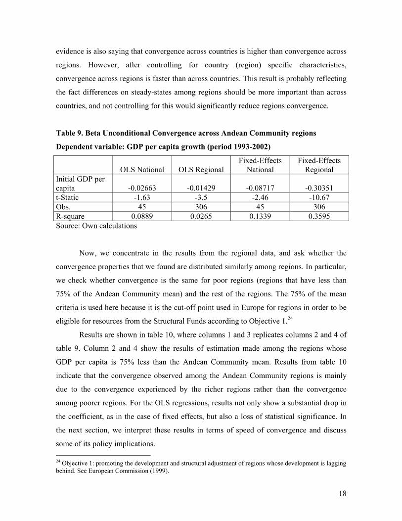
Table 9. Beta Unconditional Convergence across Andean Community regions

Dependent variable: GDP per capita growth (period 1993-2002)

OLS National OLS Regional Fixed-Effects

National Fixed-Effects

Regional Initial GDP per capita -0.02663 -0.01429 -0.08717 -0.30351 t-Static -1.63 -3.5 -2.46 -10.67 Obs. 45 306 45 306 R-square 0.0889 0.0265 0.1339 0.3595 Source: Own calculations

Now, we concentrate in the results from the regional data, and ask whether the

convergence properties that we found are distributed similarly among regions. In particular,

we check whether convergence is the same for poor regions (regions that have less than

75% of the Andean Community mean) and the rest of the regions. The 75% of the mean

criteria is used here because it is the cut-off point used in Europe for regions in order to be

eligible for resources from the Structural Funds according to Objective 1.24

Results are shown in table 10, where columns 1 and 3 replicates columns 2 and 4 of

table 9. Column 2 and 4 show the results of estimation made among the regions whose

GDP per capita is 75% less than the Andean Community mean. Results from table 10

indicate that the convergence observed among the Andean Community regions is mainly

due to the convergence experienced by the richer regions rather than the convergence

among poorer regions. For the OLS regressions, results not only show a substantial drop in

the coefficient, as in the case of fixed effects, but also a loss of statistical significance. In

the next section, we interpret these results in terms of speed of convergence and discuss

some of its policy implications. 24 Objective 1: promoting the development and structural adjustment of regions whose development is lagging behind. See European Commission (1999).

18

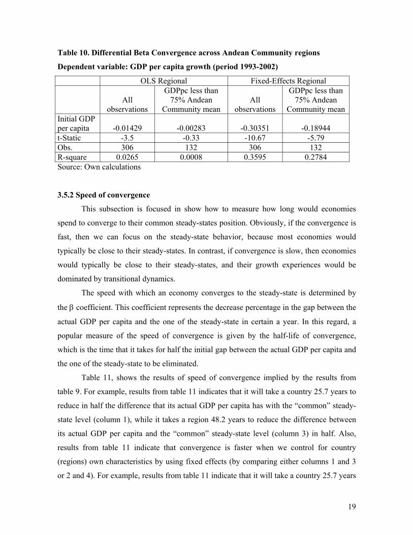
Table 10. Differential Beta Convergence across Andean Community regions

Dependent variable: GDP per capita growth (period 1993-2002)

OLS Regional Fixed-Effects Regional

All

observations

GDPpc less than 75% Andean

Community mean All

observations


Community mean Initial GDP per capita -0.01429 -0.00283 -0.30351 -0.18944 t-Static -3.5 -0.33 -10.67 -5.79 Obs. 306 132 306 132 R-square 0.0265 0.0008 0.3595 0.2784 Source: Own calculations

3.5.2 Speed of convergence

This subsection is focused in show how to measure how long would economies

spend to converge to their common steady-states position. Obviously, if the convergence is

fast, then we can focus on the steady-state behavior, because most economies would

typically be close to their steady-states. In contrast, if convergence is slow, then economies

would typically be close to their steady-states, and their growth experiences would be

dominated by transitional dynamics.

The speed with which an economy converges to the steady-state is determined by

the β coefficient. This coefficient represents the decrease percentage in the gap between the

actual GDP per capita and the one of the steady-state in certain a year. In this regard, a

popular measure of the speed of convergence is given by the half-life of convergence,

which is the time that it takes for half the initial gap between the actual GDP per capita and

the one of the steady-state to be eliminated.

Table 11, shows the results of speed of convergence implied by the results from

table 9. For example, results from table 11 indicates that it will take a country 25.7 years to

reduce in half the difference that its actual GDP per capita has with the “common” steady-

state level (column 1), while it takes a region 48.2 years to reduce the difference between

its actual GDP per capita and the “common” steady-state level (column 3) in half. Also,

results from table 11 indicate that convergence is faster when we control for country

(regions) own characteristics by using fixed effects (by comparing either columns 1 and 3

or 2 and 4). For example, results from table 11 indicate that it will take a country 25.7 years

19

to reduce in half the difference that its actual GDP per capita has with the “common”

Andean Community steady-state level (column 1), while it will take only 7.6 years to

reduce in half the difference that its actual GDP per capita has with its steady-state level

(column 3).25

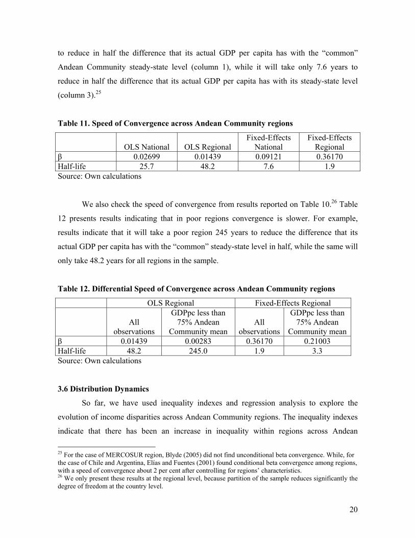
Table 11. Speed of Convergence across Andean Community regions

OLS National OLS Regional Fixed-Effects

National Fixed-Effects

Regional β 0.02699 0.01439 0.09121 0.36170 Half-life 25.7 48.2 7.6 1.9 Source: Own calculations

We also check the speed of convergence from results reported on Table 10.26 Table

12 presents results indicating that in poor regions convergence is slower. For example,

results indicate that it will take a poor region 245 years to reduce the difference that its

actual GDP per capita has with the “common” steady-state level in half, while the same will

only take 48.2 years for all regions in the sample.

Table 12. Differential Speed of Convergence across Andean Community regions

OLS Regional Fixed-Effects Regional

All

observations


Community mean All

observations


Community mean β 0.01439 0.00283 0.36170 0.21003 Half-life 48.2 245.0 1.9 3.3 Source: Own calculations

3.6 Distribution Dynamics

So far, we have used inequality indexes and regression analysis to explore the

evolution of income disparities across Andean Community regions. The inequality indexes

indicate that there has been an increase in inequality within regions across Andean

25 For the case of MERCOSUR region, Blyde (2005) did not find unconditional beta convergence. While, for the case of Chile and Argentina, Elías and Fuentes (2001) found conditional beta convergence among regions, with a speed of convergence about 2 per cent after controlling for regions’ characteristics. 26 We only present these results at the regional level, because partition of the sample reduces significantly the degree of freedom at the country level.

20

Community countries during the 1990s, but regression analysis shows evidence about the

existence of beta unconditional convergence across regions, which suggest that the

distribution of regional mean incomes might have become less polarized over time.

In order to understand the movements inside income distribution, it is important to

notice that our regression approach is to say the least limited. Quah (1995) makes this point

clear and suggest that no region can be studied in isolation independently of others. He

argues that regression-based approaches, averaging across either cross-section or time-

series dimensions, are not useful for the study of income distribution dynamics. Since, such

methods construct a (conditional) representative, and cannot provide a picture of how the

entire cross-section distribution of income evolves.

In this section, we follow Quah (1995) in the use of a distribution dynamics

approach. This approach moves away from characterizing convergence by using single

indexes or regression analyses, since it involves tracking the evolution of the entire income

distribution itself over time. We base our results in the construction of the density of the

regional per capita income distribution relative to the Andean Community average for the

year 1993. Then, we calculate how this distribution has evolve over time, in particular how

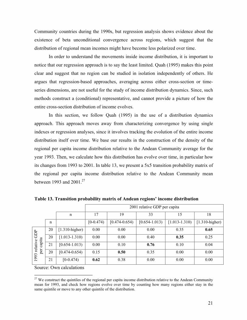
its changes from 1993 to 2001. In table 13, we present a 5x5 transition probability matrix of

the regional per capita income distribution relative to the Andean Community mean

between 1993 and 2001.27

Table 13. Transition probability matrix of Andean regions’ income distribution 2001 relative GDP per capita

n 17 19 33 15 18

n [0-0.474) [0.474-0.654) [0.654-1.013) [1.013-1.310) [1.310-higher)

20 [1.310-higher) 0.00 0.00 0.00 0.35 0.65

20 [1.013-1.310) 0.00 0.00 0.40 0.35 0.25

21 [0.654-1.013) 0.00 0.10 0.76 0.10 0.04

20 [0.474-0.654) 0.15 0.50 0.35 0.00 0.00

1993

rela

tive

GD

P pe

r cap

ita

21 [0-0.474) 0.62 0.38 0.00 0.00 0.00

Source: Own calculations 27 We construct the quintiles of the regional per capita income distribution relative to the Andean Community mean for 1993, and check how regions evolve over time by counting how many regions either stay in the same quintile or move to any other quintile of the distribution.

21

The 45 degree diagonal, numbers in bold, shows the proportion of regions that

remain in the same range of the distribution between the two years. The first row, for

example, shows that from the 20 regions that exhibited the highest GDP per capita in the

region (1.310 or higher the Andean Community average during 1993), 65% remained in the

same range in 2001, while 35% experienced a decrease in their relative position in the

income distribution.

Note that the regions in either the lower or the upper end have considerably moved

to the middle of the distribution, while regions in the middle of the distribution have a

smaller propensity to move.28 However, although regions are converging to the middle, this

is not explained by a greater growth of poorer regions but mainly for the decline

experienced by richer regions. The increase in the number of regions located at the third

quintile is explained in a larger proportion by a decline in the relative position of regions

that belonged to the fourth quintile of the distribution and have decreased its relative

position. Table 13 shows that 40% of regions in the fourth quintile dropped to the third and

only 35% of the regions in the second quintile increased to the third. If the region were

either at the lower or upper ends of the distribution in 1993, it experienced a similar

tendency to move to the upper part and the lower part of the distribution in 2001,

respectively. As a consequence, the distribution became less dense in the tails and thinner

in the middle. In other words, in 2001 there were more regions in the middle of the

distribution as compared to 1993 and fewer regions closer to the tails.

Finally, an important result, not shown in table 13, is that all the regions that

dropped from the fifth quintile to the fourth quintile are from Venezuela. Also, close to

90% of the regions that dropped from the fourth to the third quintile are from Venezuela. In

fact, only 9 of the 23 Venezuelan regions maintain its relative position while the rest reduce

its position. These results suggest that Venezuelan income distribution dynamics are very

important in explaining why Andean Community regions move from the top to the center

of the distribution.29

28 A very different result is obtained by Blyde (2005) for the case of MERCOSUR, where larger numbers in the diagonal are found, especially at the lower and upper ends. This is interpreted for the case of MERCOSUR as an indication on a very high persistence of relative regional income. 29 This evidence is consistent with Rodríguez and Sachs (1999) work that presents a model where Venezuela converges from above to its steady-state.

22

4. Conclusions

In this final section, we present some conclusion of our work and discuss some

policies that could help to reduce the agglomeration forces that are preventing the existence

of convergence between Andean regions.

Our results indicate that there has been a reduction on income disparities across

countries in the Andean Community. However, there are regional considerations that have

to be taken into account in order to have a complete picture of the convergence dynamics in

the region. At the regional level, our results indicate that inequality within countries is not

only important, it represents around 75% of the regional inequality in the Andean

Community, but has also been increasing over time. We also decompose the total change in

inequality in order to analyze the contribution of income and population changes. We find

that for the Andean Community inequality changes are mostly produced by income

changes, explaining 96% of total changes.

At the country level, it is important to mention that around 53% of the inequality

shown in the within component of the Andean Community is due to Colombia. We also

observe that within inequality in Ecuador and Peru have been reduced, while in the other

three countries, especially in Venezuela, inequality has increased. Also, for all Andean

countries, income changes are the main sources of the changes in within country inequality.

We also explore the existence of unconditional beta convergence in the Andean

Community. In general, results indicate that there exists evidence of convergence among

Andean countries (regions). This convergence is faster when we control for country

(regions) own characteristics that determine it’s steady-state level. Our results also indicate

that poor regions tend to converge slower. In fact, they indicate that it will take a poor

region 245 years to reduce the difference that its actual GDP per capita has with its steady-

state level in half, while the same will only take 48.2 years for all regions in the sample.

Our results indicate that the existence of within country differences, mainly

explained by income changes, are widening over time. They also indicate that there are

regional factors preventing poorer regions to converge faster than richer regions. We also

report results about income distribution dynamics indicating that the distribution became

less dense in the tails and thinner in the middle. In other words, in 2001 there were more

regions in the middle of the distribution as compared to 1993 and fewer regions closer to

23

the tails. However, although regions are converging to the middle, this is not explained by a

greater growth of poorer regions but mainly for the decline experienced by richer regions;

in particular the decline experienced by Venezuelan regions.

These results suggest that Andean Community countries are in need of some kind of

Structural “Cohesion” Fund. This fund could be used to revert widening regional disparities

within countries by funding infrastructure projects related to production and trade that, as

we indicated in section 2, could induce a greater effect of the dispersion forces that are

generated by the reduction of trade barriers. This could potentially prevent richer regions to

reduce its growth path and, at the same time, allow more regions to take advantage of the

increase in economic integration among Andean countries.

24

References

Barro, R. and X. Sala-i-Martin. 1995. “Economic Growth”, Mc Graw Hill.

Baldwin, F., M. Ottaviano and R. Nicoud. 2002. Manuscript for Economic Geography and

Public Policy.

Blyde, Juan. 2005. “Convergence Dynamics in Mercosur”. Inter-American Development

Bank

Cowell, F. 1995. “Measuring Inequality, Harvester Wheatsheaf”, London

Duro, J.A. 2001. “Regional income inequalities in Europe: an updated measurement and

some decomposition results”. Processed, Instituto de Análisis Económico CSIC.

Elías, Victor and Rodrigo Fuentes (2001). “Convergencia en el Cono Sur”. En

Convergencia económica e integración. Coordinated by Mancha Navarro, T., and Sotelsek

Salem, D. Ediciones Pirámide. Madrid. 2001.

European Commission. 1999. “Reform of the Structural Funds 2000-2006. Comparative

analysis”.

Hanson, G. (1998). “Regional adjustment to trade liberalization”. Regional Science and

Urban Economics, 28.

Krugman, Paul R. and Anthony J. Venables. 1990. “Integration and the competitiveness of

peripheral industry”. In Christopher Bliss and Jorge Braga de Macedo (eds.) Unity with

Diversity in the European Community. Cambridge: Cambridge University Press.

Krugman, Paul R. and Anthony J. Venables. 1996. “Integration, specialization, and

adjustment”. European Economic Review 40(3–5):959–967.

Mancha Navarro, T., and Sotelsek Salem, D. 2001. “Convergencia económica e

integración”. Ediciones Pirámide. Madrid.

Ottaviano, Gianmarco I. P. and Diego Puga. 1998. “Agglomeration in the global economy:

A survey of the ‘new economic geography’”. World Economy 21(6):707–731.

Puga, Diego and Anthony J. Venables. 1997. “Preferential trading arrangements and

industrial location”. Journal of International Economics 43(3–4):347–368.

Puga, Diego. 2001. “European regional policies in light of recent location theories”.

University of Toronto, CEPR Discussion Paper 2767.

25

Rodríguez, Francisco and Jeffrey D. Sachs. 1999. “Why Do Resource-Abundant

Economies Grow More Slowly”. September, v. 4, issue 3, pp 277-303.

Sanguinetti, P. Y Christian Volpe. (2005) , Does Trade Liberalization Favor Spatial De-

concentration of Industry?. Manuscrito.

Quah, Danny. 1995. “Regional Convergence Clusters across Europe”. Centre for Economic

Performance. Discussion Paper No.274

Venables, Anthony J. and Michael Gasiorek. 1999. “Evaluating regional infrastructure: a

computable equilibrium approach”. In Study of the Socio-economic Impact of the Projects

Financed by the Cohesion Fund — A Modelling Aproach, volume 2. Luxembourg: Office

for Official Publications of the European Communities.

26

Appendix 1. Data and sources description

1. National

• GDP(PPP): (1988-2001) in constant 1995 international $. Source: World

Development Indicators, World Bank. • Population: (1988-2001) total country. Source: World Development Indicators,

World Bank.

2. Regional30 • Bolivia:

GDP: in thousands of current bolivianos. Source: INE. Population: total regional (1993-2000). Source INE.

• Colombia: GDP: Until year 1990 in millions of constant pesos from 1975. Between 1991-2001 in millions of current pesos. Source: DANE. Population: total regional (1988-1997, 1999-2000). Source: DANE.

• Ecuador: GDP: (1993, 1996, 1999, 2001) in thousands of $. Source: BCE. Population: total regional (1990, 2001) INEC. Note: Francisco de Orellana state was included into Napo state to make data comparable across periods.

• Peru: GDP: (1988-2001) in millions of new soles from 1994. Source: APOYO Population: total regional(1990, 1993, 1995, 1997, 1998, 2000). Source: INEI.

• Venezuela: GDP: regional (states) per capita income in $ PPP (1988-2001). Source: INE, PNUD. Population: total regional(1990-2001). Source: INE. Note: Vargas state was included into Distrito Capital to make data comparable across periods.

Data manipulation

For all countries, the GDP regional shares were obtained from their national official

sources, and these were applied to the national values of GDP(PPP) in constant 1995

international US $, from the World Development Indicators (World Bank). We work with

GDP tendencies generated by the Hodrick- Prescott filter. Regional population information,

when it was not available, was estimated by using the inter-annual growth rate.31 Finally,

all the information used is annual.

30 It is important to mention that data from Household Surveys in the Andean countries are not representative at the state level, which could introduce additional problems to our estimation. 31 Specifically, we use the following formula: Vf = Vi(1+r)n.

27

Appendix 2. Regional income disparities by country

In this appendix, we analyze very briefly the Andean countries’ cross-regional

inequality by calculating the Gini, Theil and Sigma Convergence indexes for each country.

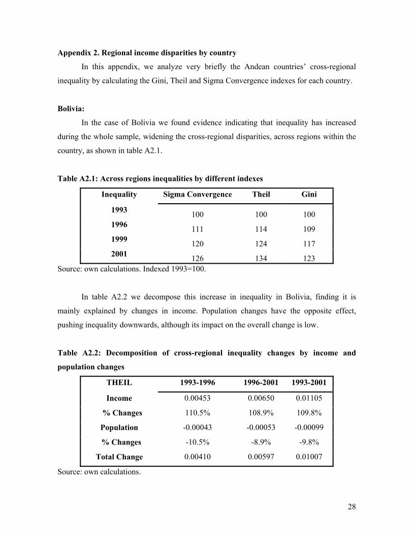
Bolivia:

In the case of Bolivia we found evidence indicating that inequality has increased

during the whole sample, widening the cross-regional disparities, across regions within the

country, as shown in table A2.1.

Table A2.1: Across regions inequalities by different indexes

Inequality Sigma Convergence Theil Gini

1993 100 100 100 1996 111 114 109 1999 120 124 117 2001 126 134 123

Source: own calculations. Indexed 1993=100.

In table A2.2 we decompose this increase in inequality in Bolivia, finding it is

mainly explained by changes in income. Population changes have the opposite effect,

pushing inequality downwards, although its impact on the overall change is low.

Table A2.2: Decomposition of cross-regional inequality changes by income and

population changes

THEIL 1993-1996 1996-2001 1993-2001

Income 0.00453 0.00650 0.01105

% Changes 110.5% 108.9% 109.8%

Population -0.00043 -0.00053 -0.00099

% Changes -10.5% -8.9% -9.8%

Total Change 0.00410 0.00597 0.01007

Source: own calculations.

28

Colombia:

In table A2.3 the three measures of inequality show an increase in inequality

between 1993 and 2001. The Sigma, Theil and Gini indexes show an increase of 5%, 8%

and 2%, respectively.


Sigma Convergence Theil Gini

1993 100 100 100 1996 102 103 101 1999 103 105 102 2001 105 108 102

Source: own calculations. Indexed 1993=100.

In table A2.4 we can observe how these changes are mostly explained by income

changes that move inequality upwards. At the same time, between 1993 and 2001

population changes move inequality upwards, especially after 1996, but its contribution to

the overall change is smaller than the contribution of income changes.

Table A2.4: Decomposition of across regional inequality changes by income and

population changes

1993-1996 1996-2001 1993-2001

Income 0.0038 0.0065 0.0106 % Changes 117% 73% 86% Population -0.0005 0.0025 0.0017

% Changes -17% 27% 14% Total Change 0.0033 0.0090 0.0122


29

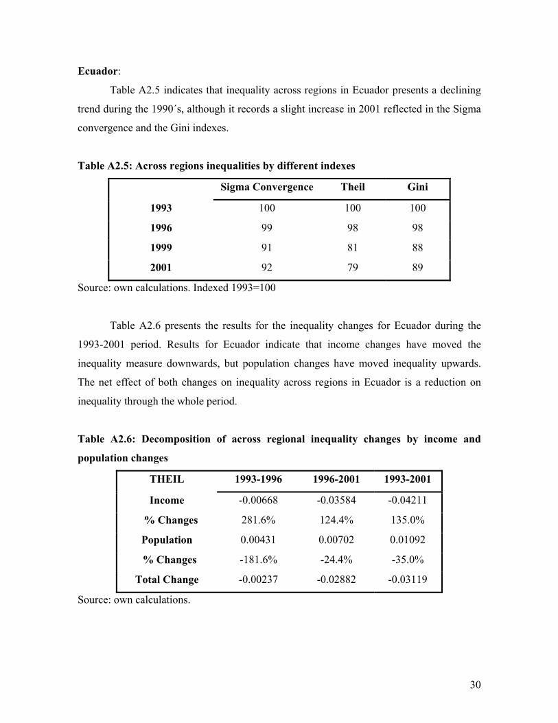
Ecuador:

Table A2.5 indicates that inequality across regions in Ecuador presents a declining

trend during the 1990´s, although it records a slight increase in 2001 reflected in the Sigma

convergence and the Gini indexes.


Sigma Convergence Theil Gini

1993 100 100 100

1996 99 98 98

1999 91 81 88

2001 92 79 89

Source: own calculations. Indexed 1993=100

Table A2.6 presents the results for the inequality changes for Ecuador during the

1993-2001 period. Results for Ecuador indicate that income changes have moved the

inequality measure downwards, but population changes have moved inequality upwards.

The net effect of both changes on inequality across regions in Ecuador is a reduction on

inequality through the whole period.


population changes

THEIL 1993-1996 1996-2001 1993-2001

Income -0.00668 -0.03584 -0.04211

% Changes 281.6% 124.4% 135.0%

Population 0.00431 0.00702 0.01092

% Changes -181.6% -24.4% -35.0%

Total Change -0.00237 -0.02882 -0.03119


30

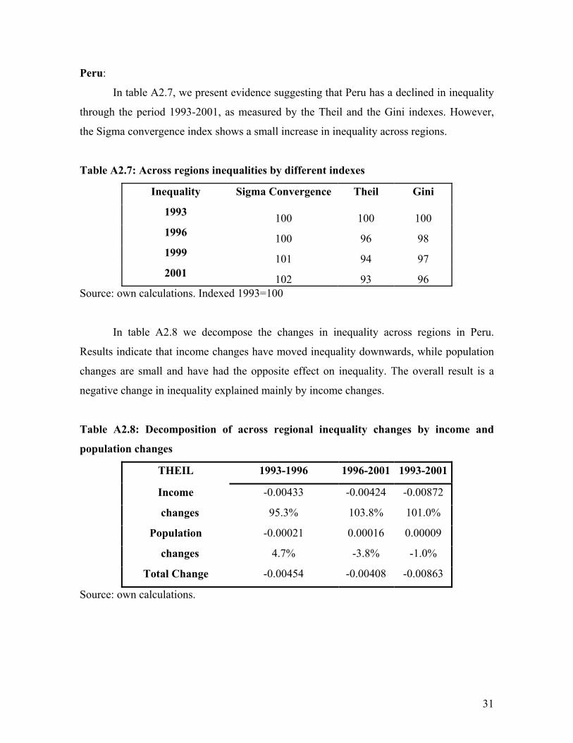
Peru:

In table A2.7, we present evidence suggesting that Peru has a declined in inequality

through the period 1993-2001, as measured by the Theil and the Gini indexes. However,

the Sigma convergence index shows a small increase in inequality across regions.



1993 100 100 100 1996 100 96 98 1999 101 94 97 2001 102 93 96


In table A2.8 we decompose the changes in inequality across regions in Peru.

Results indicate that income changes have moved inequality downwards, while population

changes are small and have had the opposite effect on inequality. The overall result is a

negative change in inequality explained mainly by income changes.


population changes

THEIL 1993-1996 1996-2001 1993-2001

Income -0.00433 -0.00424 -0.00872

changes 95.3% 103.8% 101.0%

Population -0.00021 0.00016 0.00009

changes 4.7% -3.8% -1.0%

Total Change -0.00454 -0.00408 -0.00863


31

32

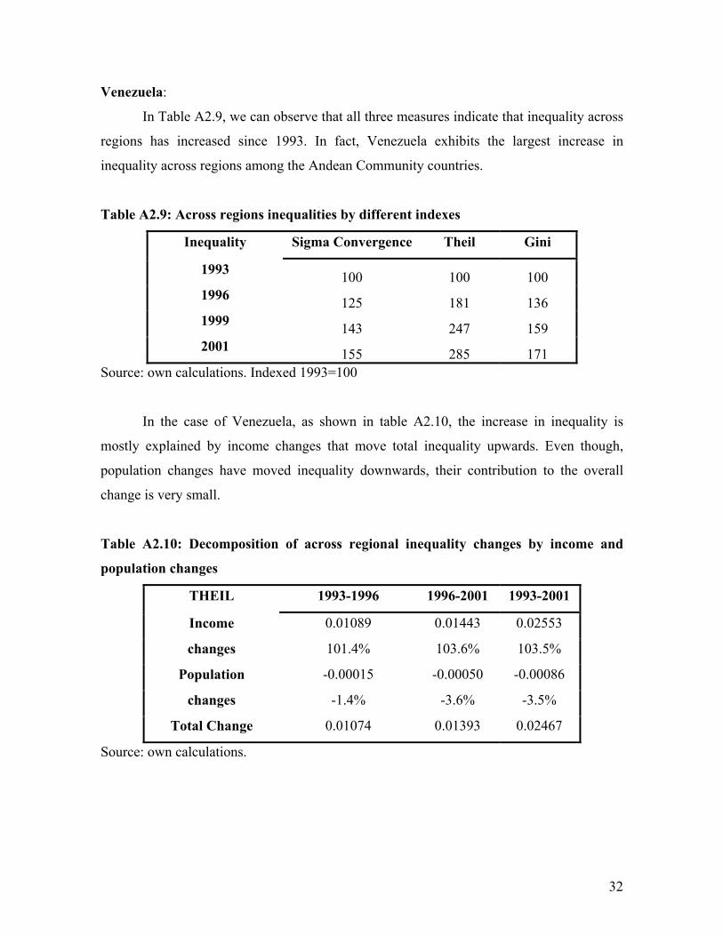
Venezuela:

In Table A2.9, we can observe that all three measures indicate that inequality across

regions has increased since 1993. In fact, Venezuela exhibits the largest increase in

inequality across regions among the Andean Community countries.



1993 100 100 100 1996 125 181 136 1999 143 247 159 2001 155 285 171


In the case of Venezuela, as shown in table A2.10, the increase in inequality is

mostly explained by income changes that move total inequality upwards. Even though,

population changes have moved inequality downwards, their contribution to the overall

change is very small.


population changes

THEIL 1993-1996 1996-2001 1993-2001

Income 0.01089 0.01443 0.02553

changes 101.4% 103.6% 103.5%

Population -0.00015 -0.00050 -0.00086

changes -1.4% -3.6% -3.5%

Total Change 0.01074 0.01393 0.02467


convergence dynamics in the andean community - … dynamics in the andean community josé pineda...

Documents