computer architecture: a constructive approach
TRANSCRIPT
Computer Architecture: A Constructive Approach
Using Executable and Synthesizable Specifications
Arvind 1, Rishiyur S. Nikhil 2,
Joel S. Emer 3, and Murali Vijayaraghavan 1
1 MIT 2 Bluespec, Inc. 3 Intel and MIT
with contributions from
Prof. Li-Shiuan Peh, Abhinav Agarwal, Elliott Fleming,Sang Woo Jun, Asif Khan, Myron King (MIT);
Prof. Derek Chiou (University of Texas, Austin);and Prof. Jihong Kim (Seoul National University)
c© 2012-2013 Arvind, R.S.Nikhil, J.Emer and M.Vijayaraghavan
Revision: December 31, 2012


Acknowledgements
We would like to thank the staff and students of various recent offerings of this course atMIT, Seoul National University and Technion for their feedback and support.
Contents
1 Introduction 1-1
2 Combinational circuits 2-1
2.1 A simple “ripple-carry” adder . . . . . . . . . . . . . . . . . . . . . . . . . . . . . . . 2-1
2.1.1 A 2-bit Ripple-Carry Adder . . . . . . . . . . . . . . . . . . . . . . . . . . . . 2-3
2.2 Static Elaboration and Static Values . . . . . . . . . . . . . . . . . . . . . . . . . . . 2-6
2.3 Integer types, conversion, extension and truncation . . . . . . . . . . . . . . . . . . . 2-7
2.4 Arithmetic-Logic Units (ALUs) . . . . . . . . . . . . . . . . . . . . . . . . . . . . . . 2-9
2.4.1 Shift operations . . . . . . . . . . . . . . . . . . . . . . . . . . . . . . . . . . . 2-9
2.4.2 Enumerated types for expressing ALU opcodes . . . . . . . . . . . . . . . . . 2-12
2.4.3 Combinational ALUs . . . . . . . . . . . . . . . . . . . . . . . . . . . . . . . . 2-13
2.4.4 Multiplication . . . . . . . . . . . . . . . . . . . . . . . . . . . . . . . . . . . . 2-14
2.5 Summary, and a word about efficient ALUs . . . . . . . . . . . . . . . . . . . . . . . 2-16
3 Sequential (Stateful) Circuits and Modules 3-1
3.1 Registers . . . . . . . . . . . . . . . . . . . . . . . . . . . . . . . . . . . . . . . . . . . 3-1
3.1.1 Space and time . . . . . . . . . . . . . . . . . . . . . . . . . . . . . . . . . . . 3-1
3.1.2 D flip-flops . . . . . . . . . . . . . . . . . . . . . . . . . . . . . . . . . . . . . 3-2
3.1.3 Registers . . . . . . . . . . . . . . . . . . . . . . . . . . . . . . . . . . . . . . 3-3
3.2 Sequential loops with registers . . . . . . . . . . . . . . . . . . . . . . . . . . . . . . 3-4
3.3 Sequential version of the multiply operator . . . . . . . . . . . . . . . . . . . . . . . 3-6
3.4 Modules and Interfaces . . . . . . . . . . . . . . . . . . . . . . . . . . . . . . . . . . . 3-7
3.4.1 Polymorphic multiply module . . . . . . . . . . . . . . . . . . . . . . . . . . . 3-11
3.5 Register files . . . . . . . . . . . . . . . . . . . . . . . . . . . . . . . . . . . . . . . . 3-12
3.6 Memories and BRAMs . . . . . . . . . . . . . . . . . . . . . . . . . . . . . . . . . . . 3-14
i
ii CONTENTS
4 Pipelining Complex Combinational Circuits 4-1
4.1 Introduction . . . . . . . . . . . . . . . . . . . . . . . . . . . . . . . . . . . . . . . . . 4-1
4.2 Pipeline registers and Inelastic Pipelines . . . . . . . . . . . . . . . . . . . . . . . . . 4-2
4.2.1 Inelastic Pipelines . . . . . . . . . . . . . . . . . . . . . . . . . . . . . . . . . 4-3
4.2.2 Stalling and Bubbles . . . . . . . . . . . . . . . . . . . . . . . . . . . . . . . . 4-4
4.2.3 Expressing data validity using the Maybe type . . . . . . . . . . . . . . . . . 4-5
4.3 Elastic Pipelines with FIFOs between stages . . . . . . . . . . . . . . . . . . . . . . . 4-8
4.4 Final comments on Inelastic and Elastic Pipelines . . . . . . . . . . . . . . . . . . . . 4-10
5 Introduction to SMIPS: a basic implementation without pipelining 5-1
5.1 Introduction to SMIPS . . . . . . . . . . . . . . . . . . . . . . . . . . . . . . . . . . . 5-1
5.1.1 Instruction Set Architectures, Architecturally Visible State, and Implementa-tion State . . . . . . . . . . . . . . . . . . . . . . . . . . . . . . . . . . . . . . 5-2
5.1.2 SMIPS processor architectural state . . . . . . . . . . . . . . . . . . . . . . . 5-2
5.1.3 SMIPS processor instruction formats . . . . . . . . . . . . . . . . . . . . . . . 5-3
5.2 Uniform interface for our processor implementations . . . . . . . . . . . . . . . . . . 5-4
5.3 A simple single-cycle implementation of SMIPS v1 . . . . . . . . . . . . . . . . . . . 5-5
5.4 Expressing our single-cycle CPU with BSV, versus prior methodologies . . . . . . . . 5-13
5.5 Separating the Fetch and Execute actions . . . . . . . . . . . . . . . . . . . . . . . . 5-15
5.5.1 Analysis . . . . . . . . . . . . . . . . . . . . . . . . . . . . . . . . . . . . . . . 5-17
6 SMIPS: Pipelined 6-1
6.1 Hazards . . . . . . . . . . . . . . . . . . . . . . . . . . . . . . . . . . . . . . . . . . . 6-1
6.1.1 Modern processors are distributed systems . . . . . . . . . . . . . . . . . . . 6-2
6.2 Two-stage pipelined SMIPS . . . . . . . . . . . . . . . . . . . . . . . . . . . . . . . . 6-2
6.2.1 A first step: a single rule, inelastic solution . . . . . . . . . . . . . . . . . . . 6-3
6.2.2 A second step: a two-rule, somewhat elastic solution . . . . . . . . . . . . . . 6-4
6.2.3 A third step: a two-rule, elastic solution using epochs . . . . . . . . . . . . . 6-5
6.2.4 A final step: a two-rule, elastic, fully-decoupled, distributed solution . . . . . 6-7
6.3 Conclusion . . . . . . . . . . . . . . . . . . . . . . . . . . . . . . . . . . . . . . . . . 6-9
7 Rule Semantics and Event Ordering 7-1
7.1 Introduction . . . . . . . . . . . . . . . . . . . . . . . . . . . . . . . . . . . . . . . . . 7-1
7.2 Parallelism: semantics of a rule in isolation . . . . . . . . . . . . . . . . . . . . . . . 7-1
7.2.1 What actions can be combined (simultaneous) in a rule? . . . . . . . . . . . . 7-2
7.2.2 Execution semantics of a single rule . . . . . . . . . . . . . . . . . . . . . . . 7-5
7.3 Logical semantics vs. implementation: sequential rule execution . . . . . . . . . . . . 7-7
7.4 Concurrent rule execution, and scheduling rules into clocks . . . . . . . . . . . . . . 7-7
iii
7.4.1 Schedules, and compilation of schedules . . . . . . . . . . . . . . . . . . . . . 7-9
7.4.2 Examples . . . . . . . . . . . . . . . . . . . . . . . . . . . . . . . . . . . . . . 7-9
7.4.3 Nuances due to conditionals . . . . . . . . . . . . . . . . . . . . . . . . . . . . 7-12
7.5 Hardware intuition for concurrent scheduling . . . . . . . . . . . . . . . . . . . . . . 7-12
7.6 Designing performance-critical ciruits using EHRs . . . . . . . . . . . . . . . . . . . 7-14
7.6.1 Intra-clock concurrency and semantics . . . . . . . . . . . . . . . . . . . . . . 7-15
7.6.2 EHRs . . . . . . . . . . . . . . . . . . . . . . . . . . . . . . . . . . . . . . . . 7-16
7.6.3 Implementing the counter with EHRs . . . . . . . . . . . . . . . . . . . . . . 7-17
7.7 Concurrent FIFOs . . . . . . . . . . . . . . . . . . . . . . . . . . . . . . . . . . . . . 7-18
7.7.1 Multi-element concurrent FIFOs . . . . . . . . . . . . . . . . . . . . . . . . . 7-18
7.7.2 Semantics of single element concurrent FIFOs . . . . . . . . . . . . . . . . . . 7-20
7.7.3 Implementing single element concurrent FIFOs using EHRs . . . . . . . . . . 7-22
8 Data Hazards (Read-after-Write Hazards) 8-1
8.1 Read-after-write (RAW) Hazards and Scoreboards . . . . . . . . . . . . . . . . . . . 8-1
8.2 Concurrency issues in the pipeline with register file and scoreboard . . . . . . . . . . 8-6
8.3 Write-after-Write Hazards . . . . . . . . . . . . . . . . . . . . . . . . . . . . . . . . . 8-7
8.4 Deeper pipelines . . . . . . . . . . . . . . . . . . . . . . . . . . . . . . . . . . . . . . 8-7
8.5 Conclusion . . . . . . . . . . . . . . . . . . . . . . . . . . . . . . . . . . . . . . . . . 8-8
9 Branch Prediction 9-1
9.1 Introduction . . . . . . . . . . . . . . . . . . . . . . . . . . . . . . . . . . . . . . . . . 9-1
9.2 Static Branch Prediction . . . . . . . . . . . . . . . . . . . . . . . . . . . . . . . . . . 9-2
9.3 Dynamic Branch Prediction . . . . . . . . . . . . . . . . . . . . . . . . . . . . . . . . 9-3
9.4 A first attempt at a better Next-Address Predictor (NAP) . . . . . . . . . . . . . . . 9-5
9.5 An improved BTB-based Next-Address Predictor . . . . . . . . . . . . . . . . . . . . 9-6
9.5.1 Implementing the Next-Address Predictor . . . . . . . . . . . . . . . . . . . . 9-6
9.6 Incorporating the BTB-based predictor in the 2-stage pipeline . . . . . . . . . . . . . 9-8
9.7 Direction predictors . . . . . . . . . . . . . . . . . . . . . . . . . . . . . . . . . . . . 9-9
9.8 Incorporating multiple predictors into the pipeline . . . . . . . . . . . . . . . . . . . 9-10
9.8.1 Extending our BSV pipeline code with multiple predictors . . . . . . . . . . . 9-12
9.9 Conclusion . . . . . . . . . . . . . . . . . . . . . . . . . . . . . . . . . . . . . . . . . 9-15
10 Exceptions 10-1
10.1 Introduction . . . . . . . . . . . . . . . . . . . . . . . . . . . . . . . . . . . . . . . . . 10-1
10.2 Asynchronous Interrupts . . . . . . . . . . . . . . . . . . . . . . . . . . . . . . . . . . 10-2
10.2.1 Interrupt Handlers . . . . . . . . . . . . . . . . . . . . . . . . . . . . . . . . . 10-2
10.3 Synchronous Interrupts . . . . . . . . . . . . . . . . . . . . . . . . . . . . . . . . . . 10-3
10.3.1 Using synchronous exceptions to handle complex and infrequent instructions 10-3
10.3.2 Incorporating exception handling into our single-cycle processor . . . . . . . . 10-3
10.4 Incorporating exception handling into our pipelined processor . . . . . . . . . . . . . 10-5
10.4.1 BSV code for pipeline with exception handling . . . . . . . . . . . . . . . . . 10-8
iv CONTENTS
11 Caches 11-1
11.1 Introduction . . . . . . . . . . . . . . . . . . . . . . . . . . . . . . . . . . . . . . . . . 11-1
11.2 Cache organizations . . . . . . . . . . . . . . . . . . . . . . . . . . . . . . . . . . . . 11-4
11.2.1 Replacement policies . . . . . . . . . . . . . . . . . . . . . . . . . . . . . . . . 11-6
11.2.2 Blocking and Non-blocking caches . . . . . . . . . . . . . . . . . . . . . . . . 11-6
11.3 A Blocking Cache Design . . . . . . . . . . . . . . . . . . . . . . . . . . . . . . . . . 11-7
11.4 Integrating caches into the processor pipeline . . . . . . . . . . . . . . . . . . . . . . 11-10
11.5 A Non-blocking cache for the Instruction Memory (Read-Only) . . . . . . . . . . . . 11-11
11.5.1 Completion Buffers . . . . . . . . . . . . . . . . . . . . . . . . . . . . . . . . . 11-13
11.6 Conclusion . . . . . . . . . . . . . . . . . . . . . . . . . . . . . . . . . . . . . . . . . 11-15
12 Virtual Memory 12-1
12.1 Introduction . . . . . . . . . . . . . . . . . . . . . . . . . . . . . . . . . . . . . . . . . 12-1
12.2 Different kinds of addresses . . . . . . . . . . . . . . . . . . . . . . . . . . . . . . . . 12-2
12.3 Paged Memory Systems . . . . . . . . . . . . . . . . . . . . . . . . . . . . . . . . . . 12-2
12.4 Page Tables . . . . . . . . . . . . . . . . . . . . . . . . . . . . . . . . . . . . . . . . . 12-4
12.5 Address translation and protection using TLBs . . . . . . . . . . . . . . . . . . . . . 12-5
12.6 Variable-sized pages . . . . . . . . . . . . . . . . . . . . . . . . . . . . . . . . . . . . 12-7
12.7 Handling TLB misses . . . . . . . . . . . . . . . . . . . . . . . . . . . . . . . . . . . 12-9
12.8 Handling Page Faults . . . . . . . . . . . . . . . . . . . . . . . . . . . . . . . . . . . 12-10
12.9 Recursive Page Faults . . . . . . . . . . . . . . . . . . . . . . . . . . . . . . . . . . . 12-11
12.10Integating Virtual Memory mechanisms ino the processor pipeline . . . . . . . . . . 12-12
12.11Conclusion . . . . . . . . . . . . . . . . . . . . . . . . . . . . . . . . . . . . . . . . . 12-14
13 Future Topics 13-1
13.1 Asynchronous Exceptions and Interrupts . . . . . . . . . . . . . . . . . . . . . . . . . 13-1
13.2 Out-of-order pipelines . . . . . . . . . . . . . . . . . . . . . . . . . . . . . . . . . . . 13-1
13.3 Protection and System Issues . . . . . . . . . . . . . . . . . . . . . . . . . . . . . . . 13-1
13.4 I and D Cache Coherence . . . . . . . . . . . . . . . . . . . . . . . . . . . . . . . . . 13-1
13.5 Multicore and Multicore cache coherence . . . . . . . . . . . . . . . . . . . . . . . . . 13-1
13.6 Simultaneous Multithreading . . . . . . . . . . . . . . . . . . . . . . . . . . . . . . . 13-2
13.7 Energy efficiency . . . . . . . . . . . . . . . . . . . . . . . . . . . . . . . . . . . . . . 13-2
13.8 Hardware accelerators . . . . . . . . . . . . . . . . . . . . . . . . . . . . . . . . . . . 13-2
v
A SMIPS Reference SMIPS-1
A.1 Basic Architecture . . . . . . . . . . . . . . . . . . . . . . . . . . . . . . . . . . . . . SMIPS-2
A.2 System Control Coprocessor (CP0) . . . . . . . . . . . . . . . . . . . . . . . . . . . . SMIPS-3
A.2.1 Test Communication Registers . . . . . . . . . . . . . . . . . . . . . . . . . . SMIPS-3
A.2.2 Counter/Timer Registers . . . . . . . . . . . . . . . . . . . . . . . . . . . . . SMIPS-3
A.2.3 Exception Processing Registers . . . . . . . . . . . . . . . . . . . . . . . . . . SMIPS-4
A.3 Addressing and Memory Protection . . . . . . . . . . . . . . . . . . . . . . . . . . . . SMIPS-6
A.4 Reset, Interrupt, and Exception Processing . . . . . . . . . . . . . . . . . . . . . . . SMIPS-7
A.4.1 Reset . . . . . . . . . . . . . . . . . . . . . . . . . . . . . . . . . . . . . . . . SMIPS-7
A.4.2 Interrupts . . . . . . . . . . . . . . . . . . . . . . . . . . . . . . . . . . . . . . SMIPS-7
A.4.3 Synchronous Exceptions . . . . . . . . . . . . . . . . . . . . . . . . . . . . . . SMIPS-8
A.5 Instruction Semantics and Encodings . . . . . . . . . . . . . . . . . . . . . . . . . . . SMIPS-9
A.5.1 Instruction Formats . . . . . . . . . . . . . . . . . . . . . . . . . . . . . . . . SMIPS-9
A.5.2 Instruction Categories . . . . . . . . . . . . . . . . . . . . . . . . . . . . . . . SMIPS-10
A.5.3 SMIPS Variants . . . . . . . . . . . . . . . . . . . . . . . . . . . . . . . . . . SMIPS-15
A.5.4 Unimplemented Instructions . . . . . . . . . . . . . . . . . . . . . . . . . . . . SMIPS-15
A.6 Instruction listing for SMIPS . . . . . . . . . . . . . . . . . . . . . . . . . . . . . . . SMIPS-16
Bibliography BIB-1

vi CONTENTS
Chapter 1
Introduction
This book is intended as an introductory course in Computer Architecture (or ComputerOrganization, or Computer Engineering) for undergraduate students who have had a basicintroduction to circuits and digital electronics. This book employs a constructive approach,i.e., all concepts are explained with machine descriptions that transparently describe archi-tecture and that can be synthesized to real hardware (for example, they can actually be runon FPGAs). Further, these descriptions will be very modular, enabling experimentationwith alternatives.
Computer Architecture has traditionally been taught with schematic diagrams and ex-planatory text. Diagrams describe general structures, such as ALUs, pipelines, caches,virtual memory mechanisms, and interconnects, or specific examples of historic machines,such as the CDC 6600, Cray-1 (recent machines are usually proprietary, meaning the de-tails of their structure may not be publicly available). These diagrams are accompanied bylectures and texts explaining principles of operation. Small quantitative exercises can bedone by hand, such as measuring cache hit rates for various cache organizations on smallsynthetic instruction streams.
In 1991, with the publication of the classic Computer Architecture: A QuantitativeApproach by Hennessy and Patterson [4] (the Fith Edition was published in 2011), the ped-agogy changed from such almost anecdotal descriptions to serious scientific, quantitativeevaluation. They firmly established the idea that architectural proposals cannot be eval-uated in the abstract, or on toy examples; they must be measured running real programs(applications, operating systems, databases, web servers, etc.) in order properly to evaluatethe engineering trade-offs (cost, performance, power, and so on). Since it has typically notbeen feasible (due to lack of time, funds and skills) for students and researchers actuallyto build the hardware to test an architectural proposal, this evaluation has typically takenthe route of simulation, i.e., writing a program (say in in C or C++) that simulates thearchitecture in question. Most of the papers in leading computer architecture conferencesare supported by data gathered this way.
Unfortunately, there are several problems with simulators written in traditional pro-gramming languages like C and C++. First, it is very hard to write an accurate modelof complex hardware. Computer system hardware is massively parallel (at the level ofregisters, pipeline stages, etc.); the paralleism is very fine-grain (at the level of individualbits and clock cycles); and the parallelism is quite heterogeneous (thousands of dissimilar
1-1

1-2 Ch 1: Introduction (DRAFT)
activities). These features are not easy to express in traditional programming languages,and simulators that try to model these features end up as very complex programs. Further,in a simulator it is too easy, without realizing it, to code actions that are unrealistic orinfeasible in real hardware, such as instantaneous, simultaneous access to a global pieceof state from distributed parts of the architecture. Finally, these simulators are very farremoved from representing any kind of formal specification of an architecture, which wouldbe useful for both manual and automated reasoning about correctness, performance, power,equivalence, and so on. A formal semantics of the interfaces and behavior of architecturalcomponents would also benefit constructive experimentation, where one could more easilysubtract, replace and add architectural components in a model in order to measure theireffectiveness.
Of course, to give confidence in hardware feasibility, one could write a simulator in thesynthesizable subset of a Hardware Description Language (HDL) such as Verilog, VHDL,or the RTL level of SystemC. Unfortunately, these are very low level languages comparedto modern programming languages, requiring orders of magnitude more effort to develop,evolve and maintain simulators; they are certainly not good vehicles for experimentation.And, these languages also lack any useful notion of formal semantics.
In this book we pursue a recently available alternative. The BSV language is a high-level, fully synthesizable hardware description language with a strong formal semantic ba-sis [1, 2, 7]. It is very suitable for describing architectures precisely and succinctly, andhas all the conveniences of modern advanced programming languages such as expressiveuser-defined types, strong type checking, polymorphism, object orientation and even higherorder functions during static elaboration.
BSV’s behavioral model is based on Guarded Atomic Actions (or atomic transactional“rules”). Computer architectures are full of very subtle issues of concurrency and ordering,such as dealing correctly with data hazards or multiple branch predictors in a processorpipeline, or distributed cache coherence in scalable multiprocessors. BSV’s formal behav-ioral model is one of the best vehicles with which to study and understand such topics (itseems also to be the computational model of choice in several other languages and tools forformal specification and analysis of complex hardware systems).
Modern hardware systems-on-a-chip (SoCs) have so much hardware on a single chip thatit is useful to conceptualize them and analyze them as distributed systems rather than asglobally synchronous systems (the traditional view), i.e., where architectural componentsare loosely coupled and communicate with messages, instead of attempting instantaneousaccess to global state. Again, BSV’s formal semantics are well suited to this flavor of models.
The ability to describe hardware module interfaces formally in BSV facilitates creatingreusable architectural components that enables quick experimentation with alternativesstructures, reinforcing the “constructive approach” mentioned in this book’s title.
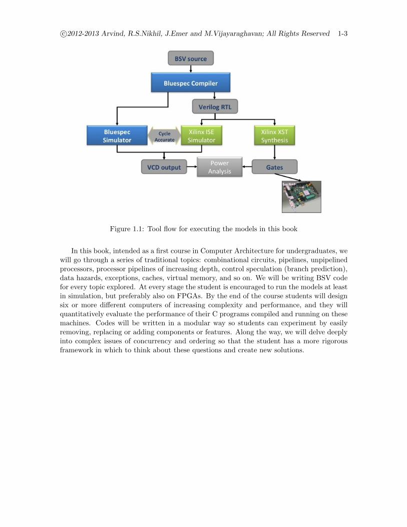
Architectural models written in BSV are fully executable. They can be simulated inthe BluesimTM simulator; they can be synthesized to Verilog and simulated on a Verilogsimulator; and they can be further synthesized to run on FPGAs, as illustrated in Fig. 1.1.This last capability is not only excellent for validating hardware feasibility of the models, butit also enables running much bigger programs on the models, since FPGA-based executioncan be 3 to 4 orders of magnitude faster than simulation. Students are also very excited tosee their designs actually running on real FPGA hardware.
c©2012-2013 Arvind, R.S.Nikhil, J.Emer and M.Vijayaraghavan; All Rights Reserved 1-3
Figure 1.1: Tool flow for executing the models in this book
In this book, intended as a first course in Computer Architecture for undergraduates, wewill go through a series of traditional topics: combinational circuits, pipelines, unpipelinedprocessors, processor pipelines of increasing depth, control speculation (branch prediction),data hazards, exceptions, caches, virtual memory, and so on. We will be writing BSV codefor every topic explored. At every stage the student is encouraged to run the models at leastin simulation, but preferably also on FPGAs. By the end of the course students will designsix or more different computers of increasing complexity and performance, and they willquantitatively evaluate the performance of their C programs compiled and running on thesemachines. Codes will be written in a modular way so students can experiment by easilyremoving, replacing or adding components or features. Along the way, we will delve deeplyinto complex issues of concurrency and ordering so that the student has a more rigorousframework in which to think about these questions and create new solutions.

1-4 Ch 1: Introduction (DRAFT)
Chapter 2
Combinational circuits
Combinational circuits are just acyclic interconnections of gates such as AND, OR, NOT,XOR, NAND, and NOR. In this chapter, we will describe the design of some Arithmetic-Logic Units (ALUs) built out of pure combinational circuits. These are the core“processing”circuits in a processor. Along the way, we will also introduce some BSV notation, types andtype checking.
2.1 A simple “ripple-carry” adder
Our goal is to build an adder that takes two w-bit input integers and produces a w-bitoutput integer plus a “carry” bit (typically, w = 32 or 64 in modern processors). First weneed a building block called a “full adder” whose inputs are the two jth bits of the twoinputs, along with the “carry” bit from the addition of the lower-order bits (up to the j−1th
bit). Its outputs are jth bit of the result, along with the carry bit up to this point. Itsfunctionality is specified by a classical “truth table”:
Inputs Outputs
a b c in c out s
0 0 0 0 00 1 0 0 11 0 0 0 11 1 0 1 00 0 1 0 10 1 1 1 01 0 1 1 01 1 1 1 1
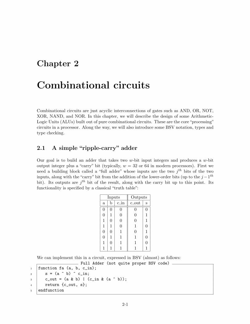
We can implement this in a circuit, expressed in BSV (almost) as follows:Full Adder (not quite proper BSV code)
1 function fa (a, b, c_in);
2 s = (a ^ b) ^ c_in;
3 c_out = (a & b) | (c_in & (a ^ b));
4 return {c_out, s};
5 endfunction
2-1
2-2 Ch 2: Combinational circuits (DRAFT)
Figure 2.1: Full adder circuit
In BSV, as in C, the &, | and ^, symbols stand for the AND, OR, and XOR (exclusiveOR) functions on bits. The circuit it describes is shown in Fig. 2.1, which is in some sensejust a pictorial depiction of the code.
A note about common sub-expressions: the code has two instances of the ex-pression (a ^ b) (on lines 2 and 3), but the circuit shows just one such gate (top-left ofthe circuit), whose output is fed to two places. Conversely, the circuit could have beendrawn with two instances of the gate, or the expression-sharing could have been suggestedexplicitly in the BSV code:
Common sub-expressions1 ...
2 tmp = (a ^ b);
3 s = tmp ^ c_in;
4 c_out = (a & b) | (c_in & tmp);
5 ...
From a functional point of view, these differences are irrelevant, since they all implementthe same truth table. From an implementation point of view it is quite relevant, since ashared gate occupies less silicon but drives a heavier load. However, we do not worryabout this issue at all when writing BSV code because the Bluespec compiler bsc performsextensive and powerful identification and unification of common-sub-expressions, no matterhow you write it. Such sharing is almost always good for implementation. Very occasionally,considerations of high fan-out and long wire-lengths may dictate otherwise; BSV has waysof specifying this, if necessary. (end of note)
The code above is not quite proper BSV, because we have not yet declared the typesof the arguments, results and intermediate variables. Here is a proper BSV version of thecode:
Full Adder (with types)1 function Bit#(2) fa (Bit#(1) a, Bit#(1) b, Bit#(1) c_in);
2 Bit#(1) s = (a ^ b) ^ c_in;
3 Bit#(1) c_out = (a & b) | (c_in & (a ^ b));
4 return {c_out,s};
5 endfunction
BSV is a strongly typed language, following modern practice for robust, scalable pro-gramming. All expressions (including variables, functions, modules and interfaces) have
c©2012-2013 Arvind, R.S.Nikhil, J.Emer and M.Vijayaraghavan; All Rights Reserved 2-3
unique types, and the compiler does extensive type checking to ensure that all operationshave meaningful types. In the above code, we’ve declared the types of all arguments and thetwo intermediate variables as Bit#(1), i.e., a 1-bit value. The result type of the functionhas been declared Bit#(2), a 2-bit value. The expression {c_out,s} represents a concate-nation of bits. The type checker ensures that all operations are meaningful, i.e., that theoperand and result types are proper for the operator (for example, it would be meaninglessto apply the square root function to an Ethernet header packet!).
BSV also has extensive type deduction or type inference, by which it can fill in typesomitted by the user. Thus, the above code could also have been written as follows:
Full Adder (with some omitted types)1 function Bit#(2) fa (Bit#(1) a, Bit#(1) b, Bit#(1) c_in);
2 let s = (a ^ b) ^ c_in;
3 let c_out = (a & b) | (c_in & (a ^ b));
4 return {c_out,s};
5 endfunction
The keyword let indicates that we would like the compiler to work out the types forus. For example, knowing the types of a, b and c_in, and knowing that the ^ operatortakes two w-bit arguments to return a w-bit result, the compiler can deduce that s has typeBit#(1).
Type-checking in BSV is much stronger than in languages like C and C++. For example,one can write an assignment statement in C or C++ that adds a char, a short, a long anda long long and assign the result to a short variable. During the additions, the values aresilently “promoted” to longer values and, during the assignment, the longer value is silentlytruncated to fit in the shorter container. The promotion may be done using zero-extensionor sign-extension, depending on the types of the operands. This kind of silent type “casting”(with no visible type checking error) is the source of many subtle bugs; even C/C++ expertsare often surprised by it. In hardware design, these errors are magnified by the fact that,unlike C/C++, we are not just working with a few fixed sizes of values (1, 2, 4 and 8 bytes)but with arbitrary bit widths in all kinds of combinations. Further, to minimize hardwarethese bit sizes are often chosen to be just large enough for the job, and so the chances ofsilent overlow and truncation are greater. In BSV, type casting is never silent, it must beexplicitly stated by the user.
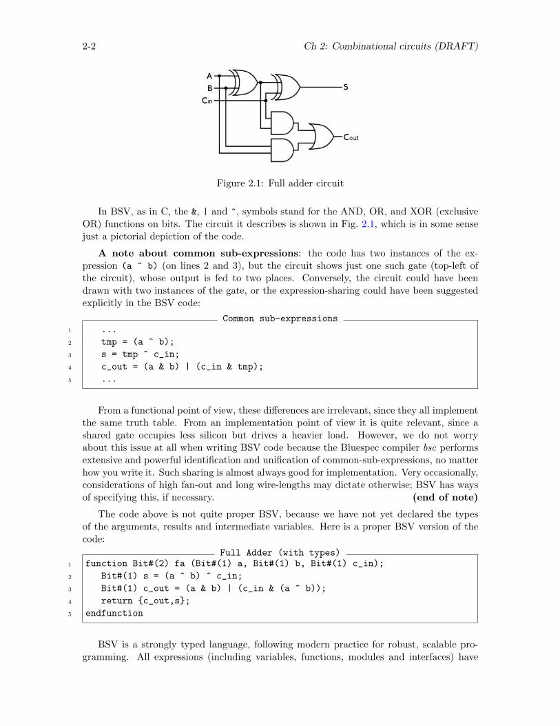
2.1.1 A 2-bit Ripple-Carry Adder
Figure 2.2: 2-bit Ripple Carry Adder circuit
2-4 Ch 2: Combinational circuits (DRAFT)
We now use our Full Adder as a black box for our next stepping stone towards a w-bitripple-carry adder: a 2-bit ripple-carry adder. The circuit is shown in Fig. 2.2, and it isdescribed by the following BSV code.
2-bit Ripple Carry Adder1 function Bit#(3) add(Bit#(2) x, Bit#(2) y, Bit#(1) c0);
2 Bit#(2) s;
3 Bit#(3) c = {?,c0};
4
5 let cs0 = fa(x[0], y[0], c[0]);
6 c[1] = cs0[1]; s[0] = cs0[0];
7
8 let cs1 = fa(x[1], y[1], c[1]);
9 c[2] = cs1[1]; s[1] = cs1[0];
10
11 return {c[2],s};
12 endfunction
Here, x and y represent the two 2-bit inputs, and c0 the input carry bit. The notationx[j] represents its jth bit, with the common convention that j = 0 is the least significantbit. We declare a 2-bit value s and a 3-bit value c to hold some intermediate values. Thelatter is initialized to the value of the expression {?,c0}. This is a bit-concatenation of twovalues, one that is left unspecified, and c0. The compiler can deduce that the unspecifiedvalue must be of type Bit#(2), since the whole expression must have type Bit#(3) and c0
has type Bit#(1).
In BSV, the expression ? represents an unspecified or “don’t care” value, leaving it up tothe compiler to choose. Here we leave it unspecified since we’re going to set the values in thesubsequent code. Similarly, the initial value of s is also unspecified by not even providingan initializer.
A full adder instance is applied to the two lower bits of x and y and the input carry bitproducing 2 bits, cs0. We assign its bits into c[1] and s[0]. A second full adder instanceis applied to the two upper bits of x and y and the carry bit of cs0 to produce 2 bits, cs1.Again, we capture those bits in c[2] and s[1]. Finally, we construct the 3-bit result fromc[2] and s. The type checker will be happy with this bit-concatenation since the widthsadd up correctly.
The types Bit#(1), Bit#(2), Bit#(3) etc. are instances of a more general type Bit#(n),where n is a“type variable”. Such types are variously called parameterized types, polymorphictypes, or generic types, because they represent a class of types, corresponding to each possibleconcrete instantiation of the type variable.
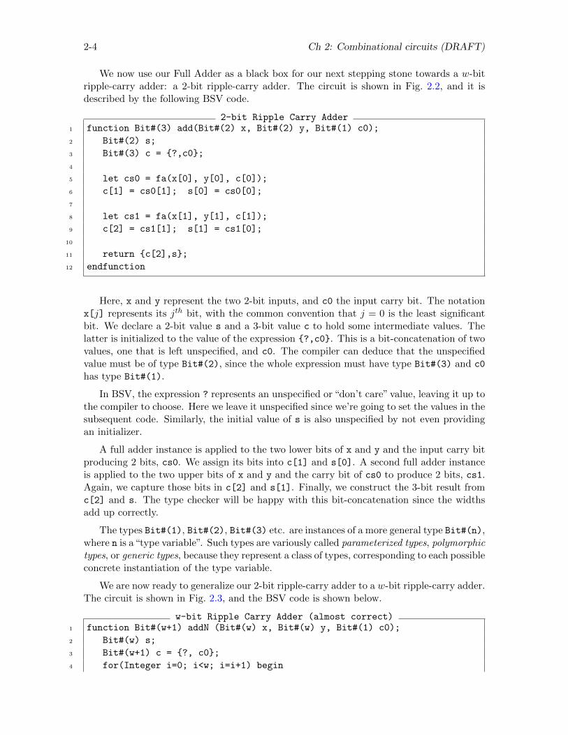
We are now ready to generalize our 2-bit ripple-carry adder to a w-bit ripple-carry adder.The circuit is shown in Fig. 2.3, and the BSV code is shown below.
w-bit Ripple Carry Adder (almost correct)1 function Bit#(w+1) addN (Bit#(w) x, Bit#(w) y, Bit#(1) c0);
2 Bit#(w) s;
3 Bit#(w+1) c = {?, c0};
4 for(Integer i=0; i<w; i=i+1) begin
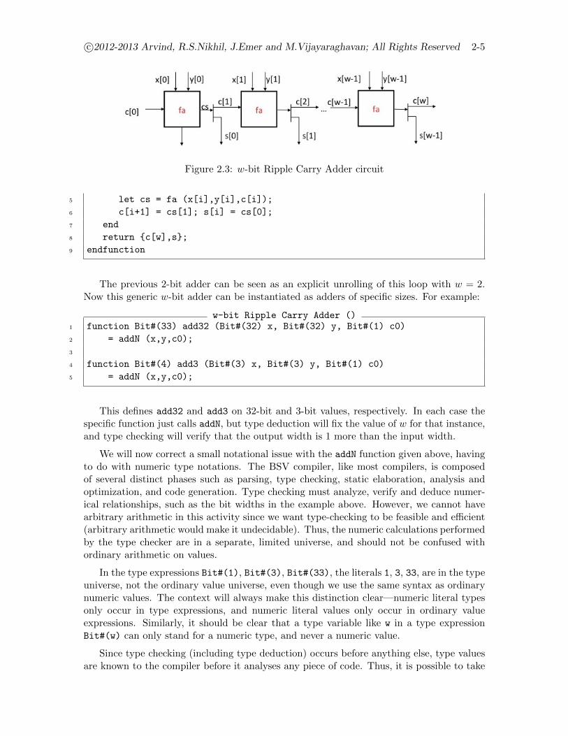
c©2012-2013 Arvind, R.S.Nikhil, J.Emer and M.Vijayaraghavan; All Rights Reserved 2-5
Figure 2.3: w-bit Ripple Carry Adder circuit
5 let cs = fa (x[i],y[i],c[i]);
6 c[i+1] = cs[1]; s[i] = cs[0];
7 end
8 return {c[w],s};
9 endfunction
The previous 2-bit adder can be seen as an explicit unrolling of this loop with w = 2.Now this generic w-bit adder can be instantiated as adders of specific sizes. For example:
w-bit Ripple Carry Adder ()1 function Bit#(33) add32 (Bit#(32) x, Bit#(32) y, Bit#(1) c0)
2 = addN (x,y,c0);
3
4 function Bit#(4) add3 (Bit#(3) x, Bit#(3) y, Bit#(1) c0)
5 = addN (x,y,c0);
This defines add32 and add3 on 32-bit and 3-bit values, respectively. In each case thespecific function just calls addN, but type deduction will fix the value of w for that instance,and type checking will verify that the output width is 1 more than the input width.
We will now correct a small notational issue with the addN function given above, havingto do with numeric type notations. The BSV compiler, like most compilers, is composedof several distinct phases such as parsing, type checking, static elaboration, analysis andoptimization, and code generation. Type checking must analyze, verify and deduce numer-ical relationships, such as the bit widths in the example above. However, we cannot havearbitrary arithmetic in this activity since we want type-checking to be feasible and efficient(arbitrary arithmetic would make it undecidable). Thus, the numeric calculations performedby the type checker are in a separate, limited universe, and should not be confused withordinary arithmetic on values.
In the type expressions Bit#(1), Bit#(3), Bit#(33), the literals 1, 3, 33, are in the typeuniverse, not the ordinary value universe, even though we use the same syntax as ordinarynumeric values. The context will always make this distinction clear—numeric literal typesonly occur in type expressions, and numeric literal values only occur in ordinary valueexpressions. Similarly, it should be clear that a type variable like w in a type expressionBit#(w) can only stand for a numeric type, and never a numeric value.
Since type checking (including type deduction) occurs before anything else, type valuesare known to the compiler before it analyses any piece of code. Thus, it is possible to take
2-6 Ch 2: Combinational circuits (DRAFT)
numeric type values from the types universe into the ordinary value universe, and use themthere (but not vice versa). The bridge is a built-in pseudo-function called valueOf(n).Here, n is a numeric type expression, and the value of the function is an ordinary Integer
value equivalent to the number represented by that type.
Numeric type expressions can also be manipulated by numeric type operators likeTAdd#(t1,t2) and TMul#(t1,t2), corresponding to addition and subtraction, respectively(other available operators include min, max, exponentiation, base-2 log, and so on).
With this in mind, we can fix up our w-bit ripple carry adder code:
w-bit Ripple Carry Adder (corrected)1 function Bit#(TAdd#(w,1)) addN (Bit#(w) x, Bit#(w) y, Bit#(1) c0);
2 Bit#(w) s;
3 Bit#(TAdd#(w,1)) c = {?, c0};
4 for(Integer i=0; i< valueOf(w); i=i+1) begin
5 let cs = fa (x[i],y[i],c[i]);
6 c[i+1] = cs[1]; s[i] = cs[0];
7 end
8 return {c[w],s};
9 endfunction
The only differences from the earlier, almost correct version is that we have usedTAdd#(w,1) instead of w+1 in lines 1 and 3 and we have inserted valueOf() in line 4.
2.2 Static Elaboration and Static Values
The w-bit ripple carry adder in the previous section illustrated how we can use syntacticfor-loops to represent repetitive circuit structures. Conceptually, the compiler “unfolds”such loops into an acyclic graph representing a (possibly large) combinational circuit. Thisprocess in the compiler is called static elaboration. In fact, in BSV you can even writerecursive functions that will be statically unfolded to represent, for example, a tree-shapedcircuit.
Of course, this unfolding needs to terminate statically (during compilation), i.e., theconditions that control the unfolding cannot depend on a dynamic, or run-time value (avalue that is only known when the circuit itself runs in hardware, or is simulated in asimulator). For example, if we wrote a for-loop whose termination index was such a run-time value, or a recursive function whose base case test depended on such a run-time value,such a loop/function could not be unfolded statically. Thus, static elaboration of loops andrecursion must only depend on static values (values known during compilation).
This distinction of static elaboration vs. dynamic execution is not something that soft-ware programmers typically think about, but it is an important topic in hardware design.In software, a recursive function is typically implemented by “unfolding” it into a stack offrames, and this stack grows and shrinks dynamically; in addition, data is communicatedbetween frames, and computation is done on this data. In a corresponding hardware imple-mentation, on the other hand, the function may be statically unfolded by the compiler intoa tree of modules (corresponding to pre-elaborating the software stack of frames), and only
c©2012-2013 Arvind, R.S.Nikhil, J.Emer and M.Vijayaraghavan; All Rights Reserved 2-7
the data communication and computation happens dynamically. Similarly, the for-loop inthe w-bit adder, if written in C, would typically actually execute as a sequential loop, dy-namically, whereas what we have seen is that our loop is statically expanded into repetitivehardware structures, and only the bits flow through it dynamically.
Of course, it is equally possible in hardware as well to implement recursive structuresand loops dynamically (the former by pushing and popping frames or contexts in memory,the latter with FSMs), mimicing exactly what software does. In fact, later we shall seethe BSV “FSM” sub-language where we can express dynamic sequential loops with dynamicbounds. But this discussion is intended to highlight the fact that hardware designers usuallythink much more carefully about what structures should/will be statically elaborated vs.what remains to execute dynamically.
To emphasize this point a little further, let us take a slight variation of our w-bit adder,in which we do not declare c as a Bit#(TAdd#(w,1)) bit vector:
w-bit Ripple Carry Adder (variation)1 function Bit#(w+1) addN (Bit#(w) x, Bit#(w) y, Bit#(1) c);
2 Bit#(w) s;
3 for(Integer i=0; i<w; i=i+1) begin
4 let cs = fa (x[i],y[i],c);
5 c = cs[1]; s[i] = cs[0];
6 end
7 return {c,s};
8 endfunction
Note that c is declared as an input parameter; it is “repeatedly updated” in the loop,and it is returned in the final result. The traditional software view of this is that c refersto a location in memory which is repeatedly updated as the loop is traversed sequentially,and whatever value finally remains in that location is returned in the result.
In BSV, c is just a name for value (there is no memory involved here, let alone anyconcept of c being a name for a location in memory that can be updated). The loop isstaticaly elaborated, and the “update” of c is just a notational device to say that this iswhat c now means for the rest of the elaboration. In fact this code, and the previousversion where c was declared as Bit#(TAdd#(w,1)) are both statically elaborated intoidentical hardware.
Over time, it becomes second nature to the BSV programmer to think of variables inthis way, i.e., not the traditional software view as an assignable location, but the purer viewof being simply a name for a value during static elaboration (ultimately, a name for a setof wires).1
2.3 Integer types, conversion, extension and truncation
One particular value type in BSV, Integer is only available as a static type for staticvariables. Semantically, these are true mathematical unbounded integers, not limited to
1For compiler afficionados: this is a pure functional view, or Static Single Assignement (SSA) view ofvariables.
2-8 Ch 2: Combinational circuits (DRAFT)
any arbitrary bit width like 32, 64, or 64K (of course, they’re ultimately limited by thememory of the system your compiler runs on). However, for dynamic integer values inhardware we typically limit them to a certain bit width, such as:
Various BSV fixed-width signed and unsigned integer types1 int, Int #(32) \\ 32-bit signed integers
2 Int #(23) \\ 23-bit signed integers
3 Int #(w) \\ signed integer of polymorphic width w
4 UInt #(48) \\ 48-bit unsigned integers
5 ...
One frequently sees Integer used in statically elaborated loops; the use of this type isa further signal to remind the reader that this is a statically elaborated loop.
In keeping with BSV’s philosophy of strong type checking, the compiler never performsautomatic (silent) conversion between these various integer types; the user needs to signala desired conversion explicitly. To convert from Integer to a fixed-width integer type, oneapplies the fromInteger function. Examples:
fromInteger1 for(Integer j=0; i< 100; j=j+1) begin
2 Int #(32) x = fromInteger (j /4);
3 UInt #(17) y = fromInteger (valueOf (w) + j);
4 ...
5 end
For truncation of one fixed-size integer type to a shorter one, use the truncate function.For extension to a longer type, use zeroExtend, signExtend and extend. The latterfunction will zero-extend for unsigned types and sign-extend for signed types. Examples:
extend and truncate1 Int #(32) x = ...;
2 Int #(64) y = signExtend (x);
3 x = truncate (y);
4 y = extend (x+2); // will sign extend
Finally, wherever you really need to, you can always convert one type to another. Forexample you might declare a memory address to be of type UInt#(32), but in some cacheyou may want to treat bits [8:6] as a signed integer bank address. You’d use notation likethe following:
pack and unpack1 typedef UInt #(32) Addr;
2 typedef Int #(3) BankAddr;
3
4 Addr a = ...
5 BankAddr ba = unpack (pack (a)[8:6]);
c©2012-2013 Arvind, R.S.Nikhil, J.Emer and M.Vijayaraghavan; All Rights Reserved 2-9
The first two lines define some type synonyms, i.e., Addr and BankAddr can now beregarded as more readable synonyms for UInt#(32) abd Int#(3). The pack function con-verts the Int #(32) value a into a Bit#(32) value; we then select bits [8:6] of this, yieldinga Bit#(3) value; the unpack function then converts this into an Int#(3) value.
This last discussion is not a compromise on strong static type checking. Type conversionswill always be necessary because one always plays application-specific representational tricks(how abtract values and structures are coded in bits) that the compiler cannot possible knowabout, particularly in hardware designs. However, by making type conversions explicit inthe source code, we eliminate most of the accidental and obscure errors that creep in eitherdue to weak type checking or due to silent implicit conversions.
2.4 Arithmetic-Logic Units (ALUs)
At the heart of any processor is an ALU (perhaps more than one) that performs all theadditions, subtractions, multiplications, ANDs, ORs, comparisons, shifts, and so on, theoperations on which computations are built. In the previous sections we had a glimpse ofbuilding one such operation—an adder. In this section we look at a few more operations,which we then combine into an ALU.
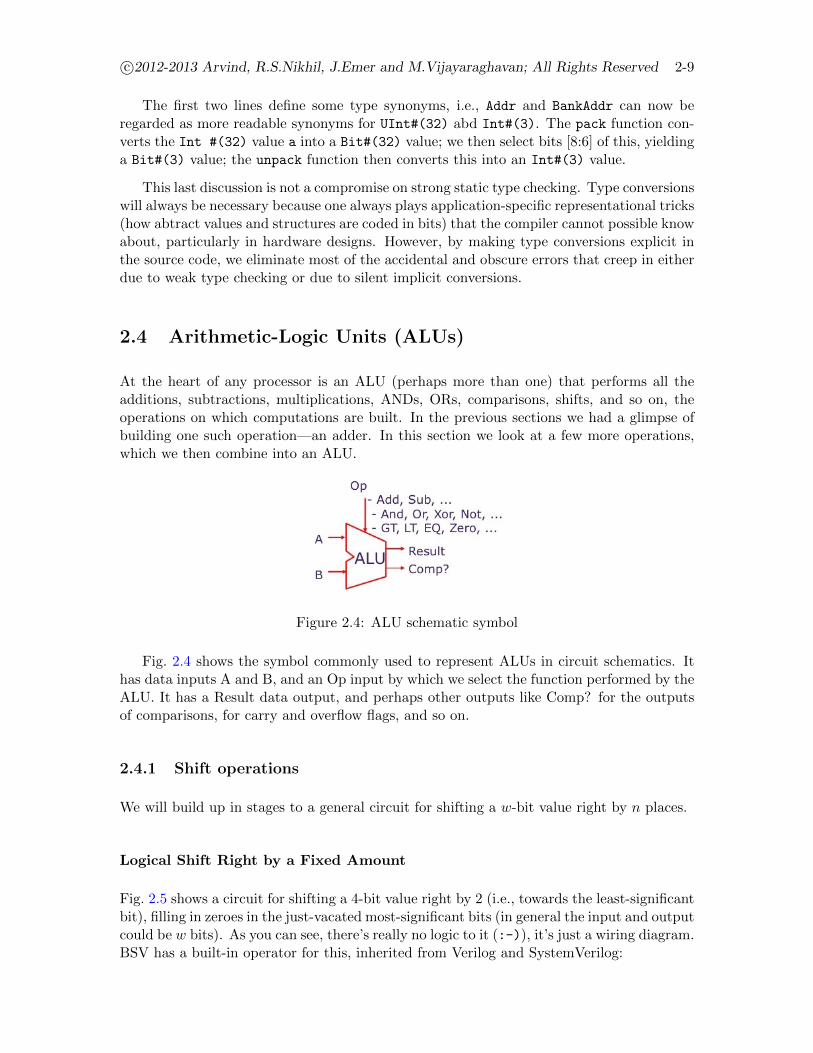
Figure 2.4: ALU schematic symbol
Fig. 2.4 shows the symbol commonly used to represent ALUs in circuit schematics. Ithas data inputs A and B, and an Op input by which we select the function performed by theALU. It has a Result data output, and perhaps other outputs like Comp? for the outputsof comparisons, for carry and overflow flags, and so on.
2.4.1 Shift operations
We will build up in stages to a general circuit for shifting a w-bit value right by n places.
Logical Shift Right by a Fixed Amount
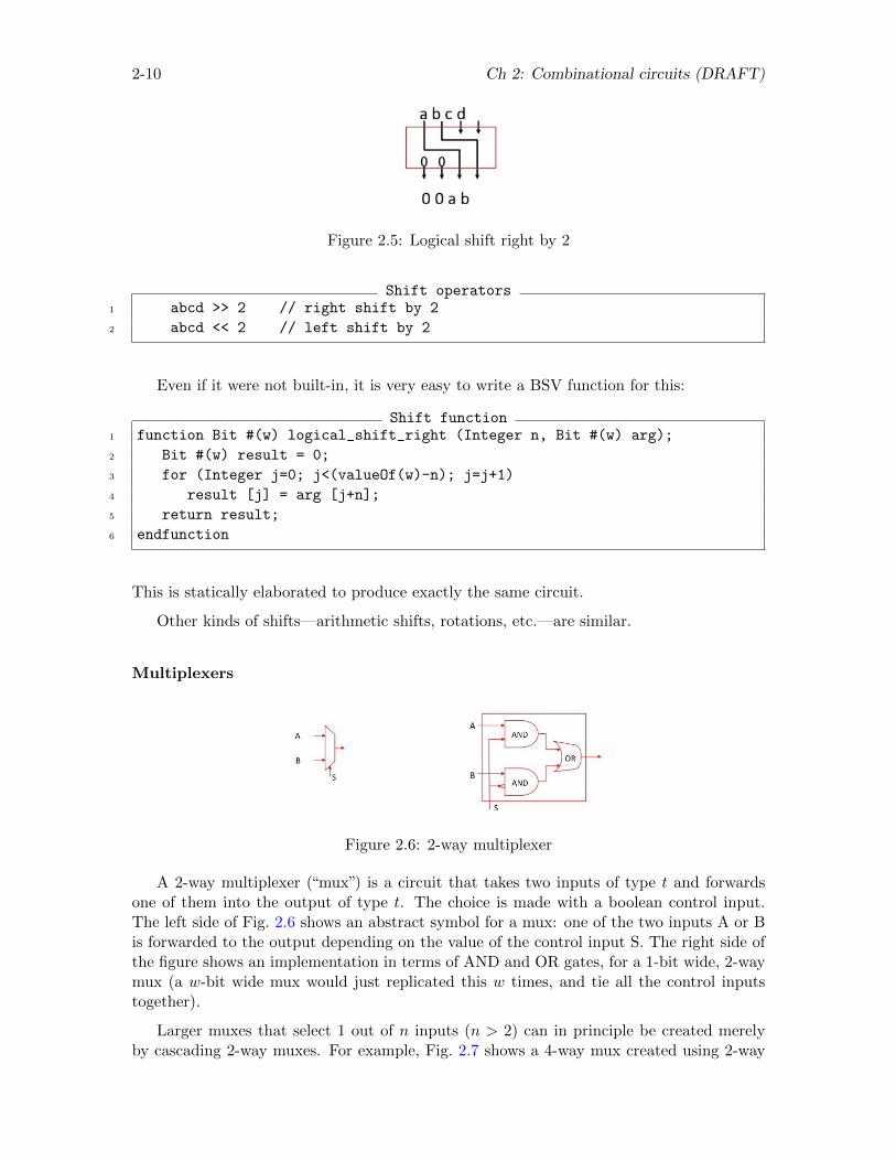
Fig. 2.5 shows a circuit for shifting a 4-bit value right by 2 (i.e., towards the least-significantbit), filling in zeroes in the just-vacated most-significant bits (in general the input and outputcould be w bits). As you can see, there’s really no logic to it (:-)), it’s just a wiring diagram.BSV has a built-in operator for this, inherited from Verilog and SystemVerilog:
2-10 Ch 2: Combinational circuits (DRAFT)
Figure 2.5: Logical shift right by 2
Shift operators1 abcd >> 2 // right shift by 2
2 abcd << 2 // left shift by 2
Even if it were not built-in, it is very easy to write a BSV function for this:
Shift function1 function Bit #(w) logical_shift_right (Integer n, Bit #(w) arg);
2 Bit #(w) result = 0;
3 for (Integer j=0; j<(valueOf(w)-n); j=j+1)
4 result [j] = arg [j+n];
5 return result;
6 endfunction
This is statically elaborated to produce exactly the same circuit.
Other kinds of shifts—arithmetic shifts, rotations, etc.—are similar.
Multiplexers
Figure 2.6: 2-way multiplexer
A 2-way multiplexer (“mux”) is a circuit that takes two inputs of type t and forwardsone of them into the output of type t. The choice is made with a boolean control input.The left side of Fig. 2.6 shows an abstract symbol for a mux: one of the two inputs A or Bis forwarded to the output depending on the value of the control input S. The right side ofthe figure shows an implementation in terms of AND and OR gates, for a 1-bit wide, 2-waymux (a w-bit wide mux would just replicated this w times, and tie all the control inputstogether).
Larger muxes that select 1 out of n inputs (n > 2) can in principle be created merelyby cascading 2-way muxes. For example, Fig. 2.7 shows a 4-way mux created using 2-way
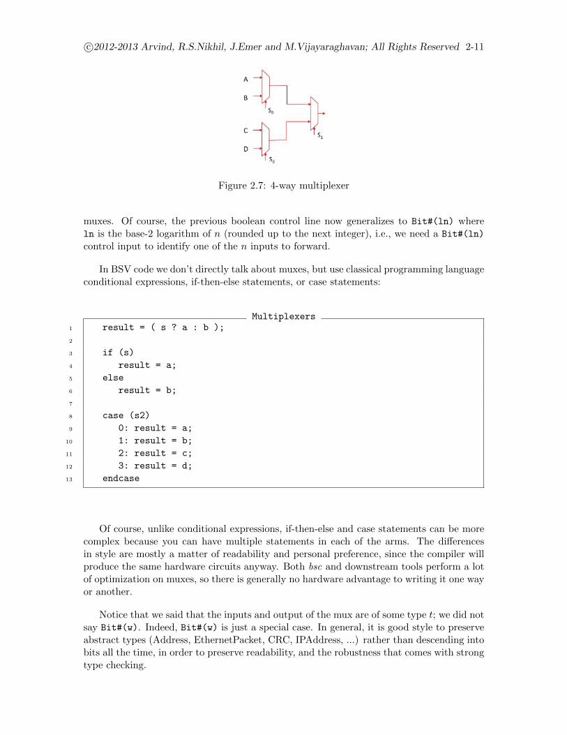
c©2012-2013 Arvind, R.S.Nikhil, J.Emer and M.Vijayaraghavan; All Rights Reserved 2-11
Figure 2.7: 4-way multiplexer
muxes. Of course, the previous boolean control line now generalizes to Bit#(ln) whereln is the base-2 logarithm of n (rounded up to the next integer), i.e., we need a Bit#(ln)
control input to identify one of the n inputs to forward.
In BSV code we don’t directly talk about muxes, but use classical programming languageconditional expressions, if-then-else statements, or case statements:
Multiplexers1 result = ( s ? a : b );
2
3 if (s)
4 result = a;
5 else
6 result = b;
7
8 case (s2)
9 0: result = a;
10 1: result = b;
11 2: result = c;
12 3: result = d;
13 endcase
Of course, unlike conditional expressions, if-then-else and case statements can be morecomplex because you can have multiple statements in each of the arms. The differencesin style are mostly a matter of readability and personal preference, since the compiler willproduce the same hardware circuits anyway. Both bsc and downstream tools perform a lotof optimization on muxes, so there is generally no hardware advantage to writing it one wayor another.
Notice that we said that the inputs and output of the mux are of some type t; we did notsay Bit#(w). Indeed, Bit#(w) is just a special case. In general, it is good style to preserveabstract types (Address, EthernetPacket, CRC, IPAddress, ...) rather than descending intobits all the time, in order to preserve readability, and the robustness that comes with strongtype checking.
2-12 Ch 2: Combinational circuits (DRAFT)
Figure 2.8: Shift by s = 0,1,2,3
Logical Shift Right by n, a Dynamic Amount
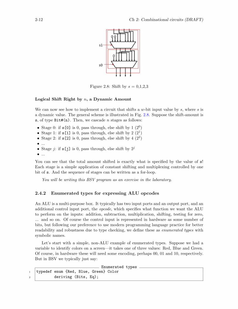
We can now see how to implement a circuit that shifts a w-bit input value by s, where s isa dynamic value. The general scheme is illustrated in Fig. 2.8. Suppose the shift-amount iss, of type Bit#(n). Then, we cascade n stages as follows:
• Stage 0: if s[0] is 0, pass through, else shift by 1 (20)• Stage 1: if s[1] is 0, pass through, else shift by 2 (21)• Stage 2: if s[2] is 0, pass through, else shift by 4 (22)• ...• Stage j: if s[j] is 0, pass through, else shift by 2j
• ...
You can see that the total amount shifted is exactly what is specified by the value of s!Each stage is a simple application of constant shifting and multiplexing controlled by onebit of s. And the sequence of stages can be written as a for-loop.
You will be writing this BSV program as an exercise in the laboratory.
2.4.2 Enumerated types for expressing ALU opcodes
An ALU is a multi-purpose box. It typically has two input ports and an output port, and anadditional control input port, the opcode, which specifies what function we want the ALUto perform on the inputs: addition, subtraction, multiplication, shifting, testing for zero,... and so on. Of course the control input is represented in hardware as some number ofbits, but following our preference to use modern programming language practice for betterreadability and robustness due to type checking, we define these as enumerated types withsymbolic names.
Let’s start with a simple, non-ALU example of enumerated types. Suppose we had avariable to identify colors on a screen—it takes one of three values: Red, Blue and Green.Of course, in hardware these will need some encoding, perhaps 00, 01 and 10, respectively.But in BSV we typically just say:
Enumerated types1 typedef enum {Red, Blue, Green} Color
2 deriving (Bits, Eq);
c©2012-2013 Arvind, R.S.Nikhil, J.Emer and M.Vijayaraghavan; All Rights Reserved 2-13
Line 1 is an enumerated type just like in C or C++, defining a new type called Color
which has three constants called Red, Blue and Green. Line 2 is a BSV incantation thattells the compiler to pick a canonical bit representation for these constants, and to definethe == and the != operators for this type, so we can compare to expressions of type Color
for equality and inequality. In fact, in this case bsc will actually choose the representations00, 01 an 10, respectively for these constants, but (a) that is an internal detail that neednot concern us, and (b) BSV has mechanisms to choose alternate encodings if we so wish.
The real payoff comes in strong type checking. Suppose, elsewhere, we have anothertype representing traffic light colors:
Enumerated types1 typedef enum {Green, Yellow, Red} TrafficLightColor
2 deriving (Bits, Eq);
These, too, will be represented using 00, 01 and 10, respectively, but strong typecheckingwill ensure that we never accidentally mix up the Color values with TrafficLightColor
values, even though both are represented using 2 bits. Any attempt to compare valuesacross these types, or to pass an argument of one of these type when the other is expected,will be caught as a static type checking error by bsc.
Processors execute instructions, which nowadays are often encoded in 32-bits. A fewfields in a 32-bit instruction usually refer to ALU opcodes of a few classes. We define themusing enumerated types like this:
Enumerated types for ALU opcodes1 typedef enum {Eq, Neq, Le, Lt, Ge, Gt, AT, NT} BrFunc
2 deriving (Bits, Eq);
3
4 typedef enum {Add, Sub, And, Or, Xor, Nor,
5 Slt, Sltu, LShift, RShift, Sra} AluFunc
6 deriving (Bits, Eq);
The first definition is for comparison operators, and the second one is for arithmetic, logicand shift operators.
2.4.3 Combinational ALUs
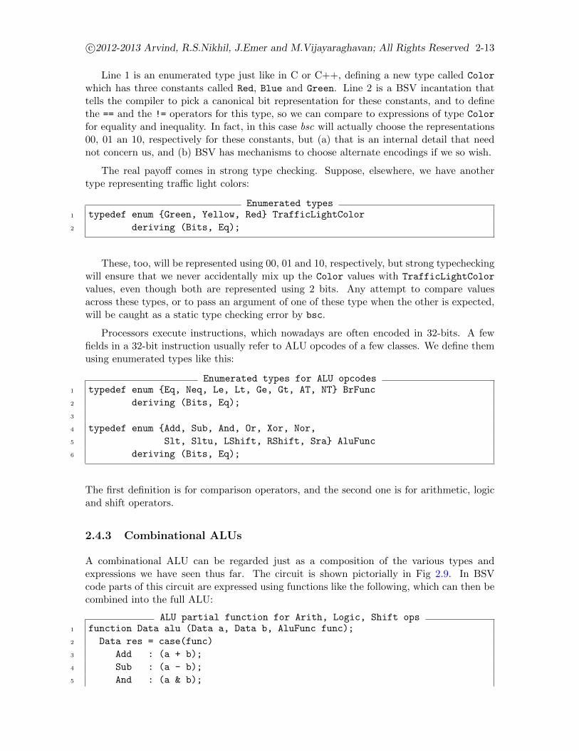
A combinational ALU can be regarded just as a composition of the various types andexpressions we have seen thus far. The circuit is shown pictorially in Fig 2.9. In BSVcode parts of this circuit are expressed using functions like the following, which can then becombined into the full ALU:
ALU partial function for Arith, Logic, Shift ops1 function Data alu (Data a, Data b, AluFunc func);
2 Data res = case(func)
3 Add : (a + b);
4 Sub : (a - b);
5 And : (a & b);
2-14 Ch 2: Combinational circuits (DRAFT)
Figure 2.9: A combinational ALU
6 Or : (a | b);
7 Xor : (a ^ b);
8 Nor : ~(a | b);
9 Slt : zeroExtend( pack( signedLT(a, b) ) );
10 Sltu : zeroExtend( pack( a < b ) );
11 LShift: (a << b[4:0]);
12 RShift: (a >> b[4:0]);
13 Sra : signedShiftRight(a, b[4:0]);
14 endcase;
15 return res;
16 endfunction
ALU partial function for Comparison1 function Bool aluBr (Data a, Data b, BrFunc brFunc);
2 Bool brTaken = case(brFunc)
3 Eq : (a == b);
4 Neq : (a != b);
5 Le : signedLE(a, 0);
6 Lt : signedLT(a, 0);
7 Ge : signedGE(a, 0);
8 Gt : signedGT(a, 0);
9 AT : True;
10 NT : False;
11 endcase;
12 return brTaken;
13 endfunction
2.4.4 Multiplication
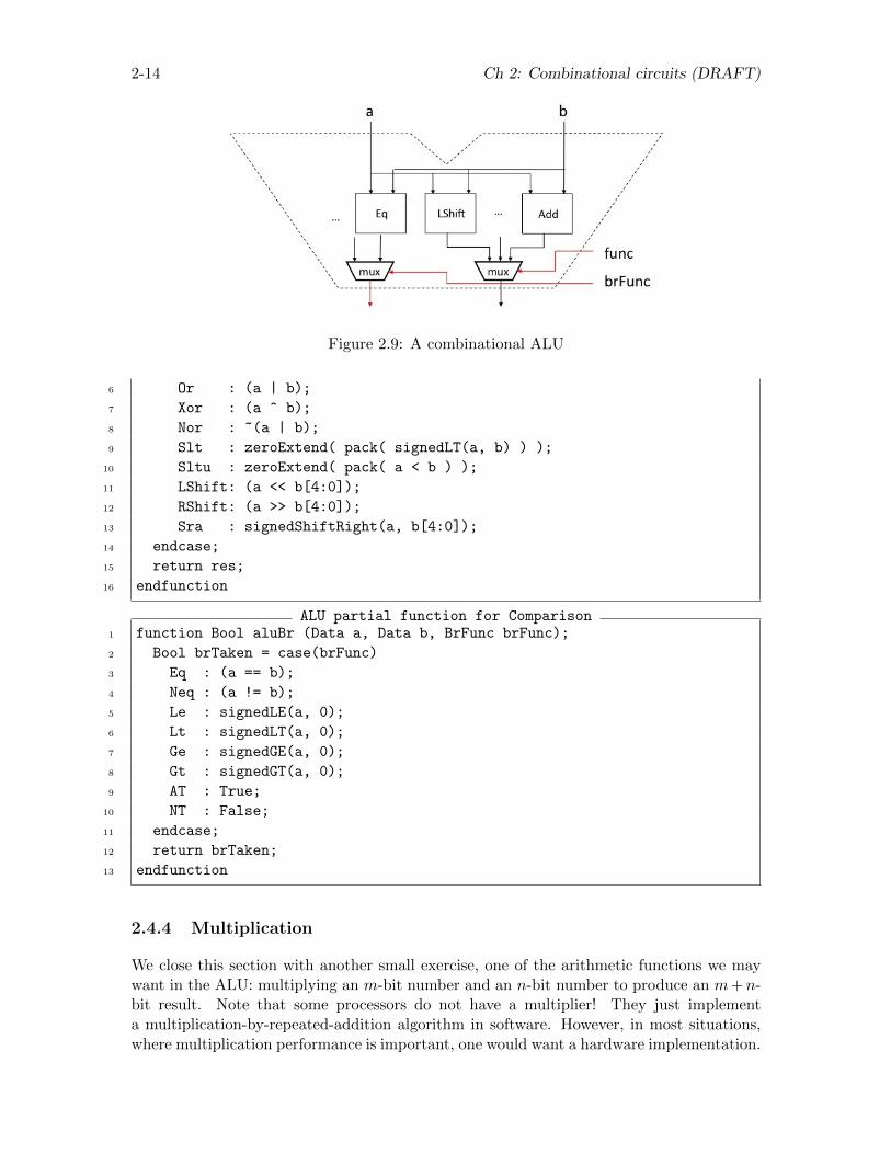
We close this section with another small exercise, one of the arithmetic functions we maywant in the ALU: multiplying an m-bit number and an n-bit number to produce an m+n-bit result. Note that some processors do not have a multiplier! They just implementa multiplication-by-repeated-addition algorithm in software. However, in most situations,where multiplication performance is important, one would want a hardware implementation.
c©2012-2013 Arvind, R.S.Nikhil, J.Emer and M.Vijayaraghavan; All Rights Reserved 2-15
Suppose were multiplying two 4-bit values together. Our high-school multiplicationalgorithm (translated from decimal to binary) looks like this:
Multiplication by repeated addition1 1 1 0 1 // Multiplicand, b
2 1 0 1 1 // Multiplier, a
3 -------
4 1 1 0 1 // b x a[0] (== b), shifted by 0
5 1 1 0 1 // b x a[1] (== b), shifted by 1
6 0 0 0 0 // b x a[2] (== 0), shifted by 2
7 1 1 0 1 // b x a[3] (== b), shifted by 3
8 ---------------
9 1 0 0 0 1 1 1 1
Thus, the jth partial sum is (a[j]==0 ? 0 : b) << j, and the overall sum is just afor-loop to add these sums. Fig. 2.10 illustrates the circuit, and here is the BSV code toexpress this:
BSV code for combinational multiplication1 function Bit#(64) mul32(Bit#(32) a, Bit#(32) b);
2 Bit#(32) prod = 0;
3 Bit#(32) tp = 0;
4 for (Integer i=0; i<32; i=i+1) begin
5 Bit#(32) m = (a[i]==0)? 0 : b;
6 Bit#(33) sum = add32(m,tp,0);
7 prod[i] = sum[0];
8 tp = truncateLSB(sum);
9 end
10 return {tp,prod};
11 endfunction
Figure 2.10: A combinational multiplier
2-16 Ch 2: Combinational circuits (DRAFT)
2.5 Summary, and a word about efficient ALUs
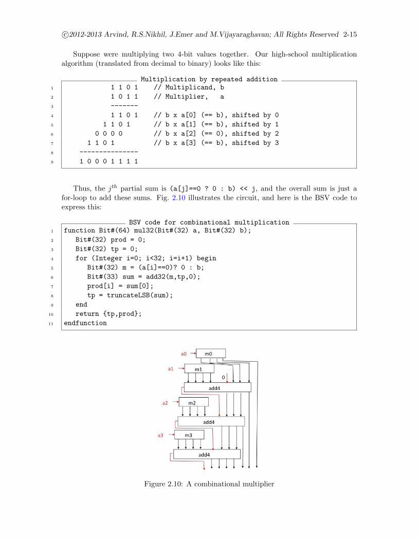
Figure 2.11: Various combinational circuits
Fig. 2.11 shows symbols for various combinational circuits. We have already discussedmultiplexers and ALUs. A demultiplexer (“demux”) transmits its input value to one of noutput ports identified by the Sel input (the other output ports are typically forced to 0).A decoder takes an input A of log n bits carrying some value 0 ≤ j ≤ 2n − 1. It has noutputs such that the jth output is 1 and all the other outputs are 0. We also say that theoutputs represent a “one-hot” bit vector, because exactly one of the outputs is 1. Thus, adecoder is equivalent to a demux where the demux’s Sel input is the decoder’s A, and thedemux’s A input is the constant 1-bit value 1.
The simple examples in this chapter of a ripple-carry adder and a simple multiplierare not meant to stand as examples of efficient design. They are merely tutorial examplesto demystify ALUs for the new student of computer architecture. Both our combinationalripple-carry adder and our combinational repeated-addition multiplier have very long chainsof gates, and wider inputs and outputs make this worse. Long combinational paths, inturn, restrict the speed of the clocks of the circuits in which we embed these ALUs, and thisultimately affects processor speeds. We may have to work, instead, with pipelined multipliersthat take multiple clock cycles to compute a result; we will discuss clocks, pipelines and soon in subsequent chapters.
In addition, modern processors also have hardware implementations for floating pointoperations, fixed point operations, transcendental functions, and more. A further concernfor the modern processor designer is power consumption. Circuit design choices for theALU can affect the power consumed per operation, and other controls may be able toswitch off power to portions of the ALU that are not currently active. In fact, the topic ofefficient computer arithmetic and ALUs has a deep and long history; people have devotedtheir careers to it, whole journals and conferences are devoted to it; here, we have barelyscratched the surface.
Chapter 3
Sequential (Stateful) Circuits andModules
3.1 Registers
3.1.1 Space and time
Recall the combinational “multiply” function from Sec. 2.4.4:
BSV code for combinational multiplication1 function Bit#(64) mul32(Bit#(32) a, Bit#(32) b);
2 Bit#(32) prod = 0;
3 Bit#(32) tp = 0;
4 for (Integer i=0; i<32; i=i+1) begin
5 Bit#(32) m = (a[i]==0)? 0 : b;
6 Bit#(33) sum = add32(m,tp,0);
7 prod[i] = sum[0];
8 tp = truncateLSB(sum);
9 end
10 return {tp,prod};
11 endfunction
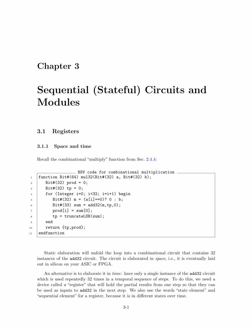
Static elaboration will unfold the loop into a combinational circuit that contains 32instances of the add32 circuit. The circuit is elaborated in space, i.e., it is eventually laidout in silicon on your ASIC or FPGA.
An alternative is to elaborate it in time: have only a single instance of the add32 circuitwhich is used repeatedly 32 times in a temporal sequence of steps. To do this, we need adevice called a “register” that will hold the partial results from one step so that they canbe used as inputs to add32 in the next step. We also use the words “state element” and“sequential element” for a register, because it is in different states over time.
3-1
3-2 Ch 3: Sequential circuits (DRAFT)
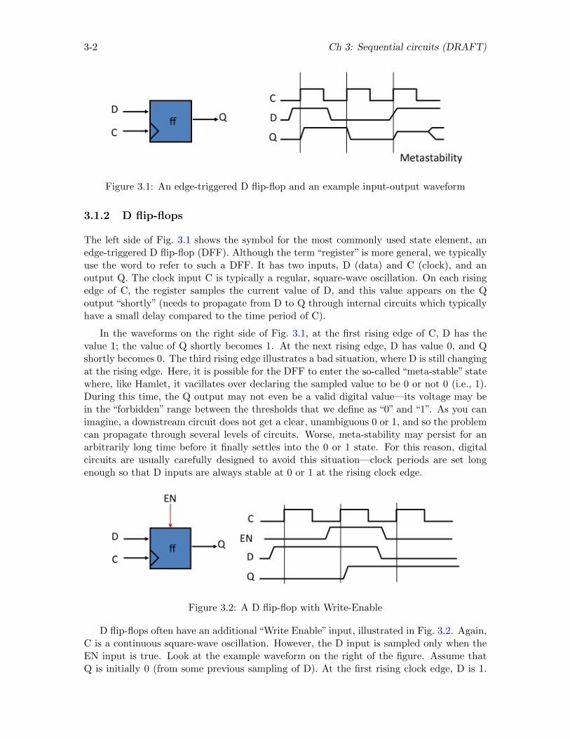
Figure 3.1: An edge-triggered D flip-flop and an example input-output waveform
3.1.2 D flip-flops
The left side of Fig. 3.1 shows the symbol for the most commonly used state element, anedge-triggered D flip-flop (DFF). Although the term “register” is more general, we typicallyuse the word to refer to such a DFF. It has two inputs, D (data) and C (clock), and anoutput Q. The clock input C is typically a regular, square-wave oscillation. On each risingedge of C, the register samples the current value of D, and this value appears on the Qoutput “shortly” (needs to propagate from D to Q through internal circuits which typicallyhave a small delay compared to the time period of C).
In the waveforms on the right side of Fig. 3.1, at the first rising edge of C, D has thevalue 1; the value of Q shortly becomes 1. At the next rising edge, D has value 0, and Qshortly becomes 0. The third rising edge illustrates a bad situation, where D is still changingat the rising edge. Here, it is possible for the DFF to enter the so-called “meta-stable” statewhere, like Hamlet, it vacillates over declaring the sampled value to be 0 or not 0 (i.e., 1).During this time, the Q output may not even be a valid digital value—its voltage may bein the “forbidden” range between the thresholds that we define as “0” and “1”. As you canimagine, a downstream circuit does not get a clear, unambiguous 0 or 1, and so the problemcan propagate through several levels of circuits. Worse, meta-stability may persist for anarbitrarily long time before it finally settles into the 0 or 1 state. For this reason, digitalcircuits are usually carefully designed to avoid this situation—clock periods are set longenough so that D inputs are always stable at 0 or 1 at the rising clock edge.
Figure 3.2: A D flip-flop with Write-Enable
D flip-flops often have an additional “Write Enable” input, illustrated in Fig. 3.2. Again,C is a continuous square-wave oscillation. However, the D input is sampled only when theEN input is true. Look at the example waveform on the right of the figure. Assume thatQ is initially 0 (from some previous sampling of D). At the first rising clock edge, D is 1.
c©2012-2013 Arvind, R.S.Nikhil, J.Emer and M.Vijayaraghavan; All Rights Reserved 3-3
However, since EN is 0, it is not sampled, and Q retains its previous value of 0. At thesecond clock edge, EN is 1, and so the value of D (1) is sampled, and arrives at Q. At thethird clock edge, EN is 0, so D (0) is not sampled, and Q remains at 1.
Figure 3.3: Implementing a D flip-flop with Write-Enable
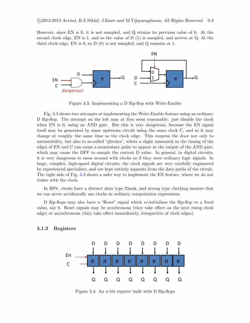
Fig. 3.3 shows two attempts at implementing the Write-Enable feature using an ordinaryD flip-flop. The attempt on the left may at first seem reasonable: just disable the clockwhen EN is 0, using an AND gate. But this is very dangerous, because the EN signalitself may be generated by some upstream circuit using the same clock C, and so it maychange at roughly the same time as the clock edge. This reopens the door not only tometastability, but also to so-called “glitches”, where a slight mismatch in the timing of theedges of EN and C can cause a momentary pulse to appear at the output of the AND gate,which may cause the DFF to sample the current D value. In general, in digital circuits,it is very dangerous to mess around with clocks as if they were ordinary logic signals. Inlarge, complex, high-speed digital circuits, the clock signals are very carefully engineeredby experienced specialists, and are kept entirely separate from the data paths of the circuit.The right side of Fig. 3.3 shows a safer way to implement the EN feature, where we do nottinker with the clock.
In BSV, clocks have a distinct data type Clock, and strong type checking ensures thatwe can never accidentally use clocks in ordinary computation expressions.
D flip-flops may also have a “Reset” signal which re-initializes the flip-flop to a fixedvalue, say 0. Reset signals may be synchronous (they take effect on the next rising clockedge) or asynchronous (they take effect immediately, irrespective of clock edges).
3.1.3 Registers
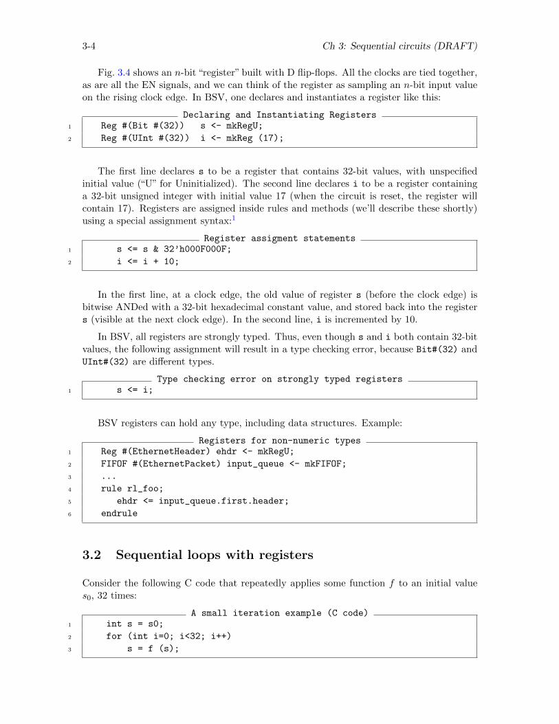
Figure 3.4: An n-bit register built with D flip-flops
3-4 Ch 3: Sequential circuits (DRAFT)
Fig. 3.4 shows an n-bit “register” built with D flip-flops. All the clocks are tied together,as are all the EN signals, and we can think of the register as sampling an n-bit input valueon the rising clock edge. In BSV, one declares and instantiates a register like this:
Declaring and Instantiating Registers1 Reg #(Bit #(32)) s <- mkRegU;
2 Reg #(UInt #(32)) i <- mkReg (17);
The first line declares s to be a register that contains 32-bit values, with unspecifiedinitial value (“U” for Uninitialized). The second line declares i to be a register containinga 32-bit unsigned integer with initial value 17 (when the circuit is reset, the register willcontain 17). Registers are assigned inside rules and methods (we’ll describe these shortly)using a special assignment syntax:1
Register assigment statements1 s <= s & 32’h000F000F;
2 i <= i + 10;
In the first line, at a clock edge, the old value of register s (before the clock edge) isbitwise ANDed with a 32-bit hexadecimal constant value, and stored back into the registers (visible at the next clock edge). In the second line, i is incremented by 10.
In BSV, all registers are strongly typed. Thus, even though s and i both contain 32-bitvalues, the following assignment will result in a type checking error, because Bit#(32) andUInt#(32) are different types.
Type checking error on strongly typed registers1 s <= i;
BSV registers can hold any type, including data structures. Example:
Registers for non-numeric types1 Reg #(EthernetHeader) ehdr <- mkRegU;
2 FIFOF #(EthernetPacket) input_queue <- mkFIFOF;
3 ...
4 rule rl_foo;
5 ehdr <= input_queue.first.header;
6 endrule
3.2 Sequential loops with registers
Consider the following C code that repeatedly applies some function f to an initial values0, 32 times:
A small iteration example (C code)1 int s = s0;
2 for (int i=0; i<32; i++)
3 s = f (s);
c©2012-2013 Arvind, R.S.Nikhil, J.Emer and M.Vijayaraghavan; All Rights Reserved 3-5
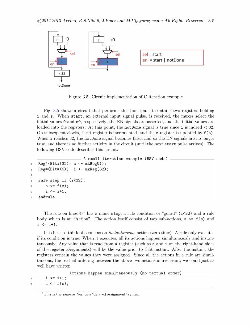
Figure 3.5: Circuit implementation of C iteration example
Fig. 3.5 shows a circuit that performs this function. It contains two registers holdingi and s. When start, an external input signal pulse, is received, the muxes select theinitial values 0 and s0, respectively; the EN signals are asserted, and the initial values areloaded into the registers. At this point, the notDone signal is true since i is indeed < 32.On subsequent clocks, the i register is incremented, and the s register is updated by f(s).When i reaches 32, the notDone signal becomes false, and so the EN signals are no longertrue, and there is no further activity in the circuit (until the next start pulse arrives). Thefollowing BSV code describes this circuit:
A small iteration example (BSV code)1 Reg#(Bit#(32)) s <- mkRegU();
2 Reg#(Bit#(6)) i <- mkReg(32);
3
4 rule step if (i<32);
5 s <= f(s);
6 i <= i+1;
7 endrule
The rule on lines 4-7 has a name step, a rule condition or “guard” (i<32) and a rulebody which is an “Action”. The action itself consist of two sub-actions, s <= f(s) andi <= i+1.
It is best to think of a rule as an instantaneous action (zero time). A rule only executesif its condition is true. When it executes, all its actions happen simultaneously and instan-taneously. Any value that is read from a register (such as s and i on the right-hand sidesof the register assignments) will be the value prior to that instant. After the instant, theregisters contain the values they were assigned. Since all the actions in a rule are simul-taneous, the textual ordering between the above two actions is irrelevant; we could just aswell have written:
Actions happen simultaneously (no textual order)1 i <= i+1;
2 s <= f(s);
1This is the same as Verilog’s “delayed assignment” syntax
3-6 Ch 3: Sequential circuits (DRAFT)
Thus, this rule acts as a sequential loop, repeatedly updating registers i and s until(i>=32). When synthesized by bsc, we get the circuit of Fig.3.5.
A small BSV nuance regarding types
Why did we declare i to have the type Bit#(6) instead of Bit#(5)? It’s because in theexpression (i<32), the literal value 32 needs 6 bits, and the comparision operator < expectsboth its operands to have the same type. If we had declared i to have type Bit#(5) wewould have got a type checking error in the expression (i<32). Suppose we try changingthe condition to (i<=31), since the literal 31 only needs 5 bits?
Types subtlety1 ...
2 Reg#(Bit#(5)) i <- ...
3
4 rule step if (i<=31);
5 ...
6 i <= i+1;
7 endrule
This program will type check and run, but it will never terminate! The reason is thatwhen i has the value 31 and we increment it to i+1, it will simply wrap around to the value0. Thus, the condition i<=31 is always true, and so the rule will fire forever. Note, the sameissue could occur in a C program as well, but since we usually use 32-bit arithmetic in Cprograms, we rarely encounter it. We need to be much more sensitive to this in hardwaredesigns, because we usually try to use the minimum number of bits adequate for the job.
3.3 Sequential version of the multiply operator
Looking at the combinational multiply operator code at the beginning of this chapter, wesee that the values that change during the loop are i, prod and tp; we will need to holdthese in registers when writing a sequential version of the loop:
BSV code for sequential multiplication1 Reg #(Bit#(32)) a <- mkRegU;
2 Reg #(Bit#(32)) b <- mkRegU;
3 Reg #(Bit#(32)) prod <- mkRegU;
4 Reg #(Bit#(32)) tp <- mkRegU;
5 Reg #(Bit#(6)) i <- mkReg (32);
6
7 rule mulStep if (i<32);
8 Bit#(32) m = (a[i]==0)? 0 : b;
9 Bit#(33) sum = add32(m,tp,0);
10 prod[i] <= sum[0]; // (not quite kosher BSV)
11 tp <= truncateLSB(sum);
12 i <= i + 1;
13 endrule
c©2012-2013 Arvind, R.S.Nikhil, J.Emer and M.Vijayaraghavan; All Rights Reserved 3-7
The register i is initialized to 32, which is the quiescent state of the circuit (no activity).To start the computation, something has to load a and b with the values to be multipliedand load prod, tp and i with their initial value of 0 (we will see this initialization later).Then, the rule fires repeatedly as long as (i<32). The first four lines of the body of therule are identical to the body of the for-loop in the combinational function at the start ofthis chapter, except that the assignments to prod[i] and tp have been changed to registerassignments.
Although functionally ok, we can improve it to a more efficient circuit by eliminatingdynamic indexing. Consider the expression a[i]. This is a 32-way mux: 32 1-bit inputwires connected to the bits of a, with i as the mux selector. However, since i is a simpleincrementing series, we could instead repeatedly shift a right by 1, and always look atthe least significant bit (LSB), effectively looking at a[0], a[1], a[2], ... Shifting by 1requires no gates (it’s just wires!), and so we eliminate a mux. Similarly, when we assign toprod[i], we need a decoder to route the value into the ith bit of prod. Instead, we couldrepeatedly shift prod right by 1, and insert the new bit at the most significant bit (MSB).This eliminates the decoder. Here is the fixed-up code:
BSV code for sequential multiplication1 Reg #(Bit#(32)) a <- mkRegU;
2 Reg #(Bit#(32)) b <- mkRegU;
3 Reg #(Bit#(32)) prod <- mkRegU;
4 Reg #(Bit#(32)) tp <- mkRegU;
5 Reg #(Bit#(6)) i <- mkReg (32);
6
7 rule mulStep if (i<32);
8 Bit#(32) m = (a[0]==0)? 0 : b; // only look at LSB of a
9 a <= a >> 1; // shift a by 1
10 Bit#(33) sum = add32(m,tp,0);
11 prod <= { sum[0], prod [31:1] }; // shift prod by 1, insert at MSB
12 tp <= truncateLSB(sum);
13 i <= i + 1;
14 endrule
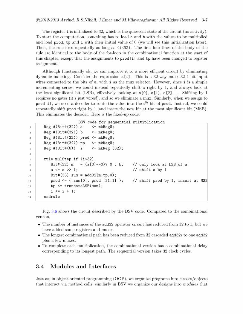
Fig. 3.6 shows the circuit described by the BSV code. Compared to the combinationalversion,
• The number of instances of the add32 operator circuit has reduced from 32 to 1, but wehave added some registers and muxes.
• The longest combinational path has been reduced from 32 cascaded add32s to one add32plus a few muxes.
• To complete each multiplication, the combinational version has a combinational delaycorresponding to its longest path. The sequential version takes 32 clock cycles.
3.4 Modules and Interfaces
Just as, in object-oriented programming (OOP), we organize programs into classes/objectsthat interact via method calls, similarly in BSV we organize our designs into modules that
3-8 Ch 3: Sequential circuits (DRAFT)
Figure 3.6: Sequential multiplication circuit
interact using methods. And in BSV, just like OOP, we separate the concept of the interfaceof a module—“What methods does it implement and what are the argument and resulttypes?”—from the module itself— “How does it implement the methods?”.
For example, if we want to package our multiplier into a module that can be instantiated(reused) multiple times, we first think about the interface it should present to the externalworld. Here is a proposed interface:
Multiplier module interface1 interface Multiply32;
2 method Action start (Bit#(32) a, Bit#(32) b);
3 method Bit#(64) result;
4 endinterface
A module with this interface offers two methods that can be invoked from outside. Thestart method takes two arguments a and b, and has Action type, namely it just performssome action (this method does not return any result). In this case, it just kicks off theinternal computation to multiply a and b, which may take many steps. The result methodhas no arguments, and returns a value of type Bit#(64).
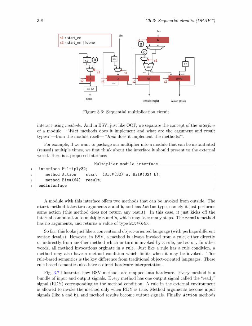
So far, this looks just like a conventional object-oriented language (with perhaps differentsyntax details). However, in BSV, a method is always invoked from a rule, either directlyor indirectly from another method which in turn is invoked by a rule, and so on. In otherwords, all method invocations orginate in a rule. Just like a rule has a rule condition, amethod may also have a method condition which limits when it may be invoked. Thisrule-based semantics is the key difference from traditional object-oriented languages. Theserule-based semantics also have a direct hardware interpretation.
Fig. 3.7 illustrates how BSV methods are mapped into hardware. Every method is abundle of input and output signals. Every method has one output signal called the “ready”signal (RDY) corresponding to the method condition. A rule in the external environmentis allowed to invoke the method only when RDY is true. Method arguments become inputsignals (like a and b), and method results become output signals. Finally, Action methods
c©2012-2013 Arvind, R.S.Nikhil, J.Emer and M.Vijayaraghavan; All Rights Reserved 3-9
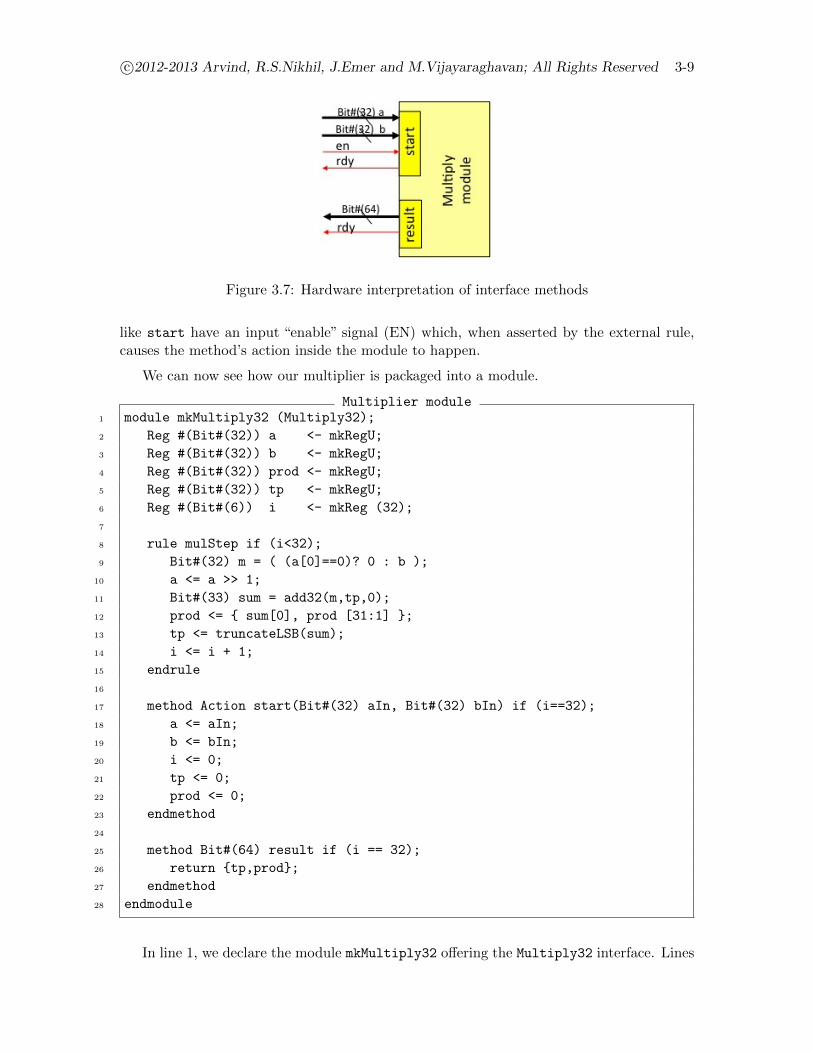
Figure 3.7: Hardware interpretation of interface methods
like start have an input “enable” signal (EN) which, when asserted by the external rule,causes the method’s action inside the module to happen.
We can now see how our multiplier is packaged into a module.
Multiplier module1 module mkMultiply32 (Multiply32);
2 Reg #(Bit#(32)) a <- mkRegU;
3 Reg #(Bit#(32)) b <- mkRegU;
4 Reg #(Bit#(32)) prod <- mkRegU;
5 Reg #(Bit#(32)) tp <- mkRegU;
6 Reg #(Bit#(6)) i <- mkReg (32);
7
8 rule mulStep if (i<32);
9 Bit#(32) m = ( (a[0]==0)? 0 : b );
10 a <= a >> 1;
11 Bit#(33) sum = add32(m,tp,0);
12 prod <= { sum[0], prod [31:1] };
13 tp <= truncateLSB(sum);
14 i <= i + 1;
15 endrule
16
17 method Action start(Bit#(32) aIn, Bit#(32) bIn) if (i==32);
18 a <= aIn;
19 b <= bIn;
20 i <= 0;
21 tp <= 0;
22 prod <= 0;
23 endmethod
24
25 method Bit#(64) result if (i == 32);
26 return {tp,prod};
27 endmethod
28 endmodule
In line 1, we declare the module mkMultiply32 offering the Multiply32 interface. Lines
3-10 Ch 3: Sequential circuits (DRAFT)
2-15 are identical to what we developed in the last section. Lines 17-23 implement thestart method. The method condition, or guard, is (i==32). When invoked, it initializesall the registers. Lines 25-27 implement the result method. Its method condition or guardis also (i==32). When invoked it returns {tp,prod} as its result.
BSV modules typically follow this organization: internal state (here, lines 2-6), followedby internal behavior (here, lines 8-15) followed by interface definitions (here, lines 17-27).As a programming convention, we typically write module names as mk..., and pronouncethe first syllable as “make”, reflecting the fact that a module can be instantiated multipletimes.
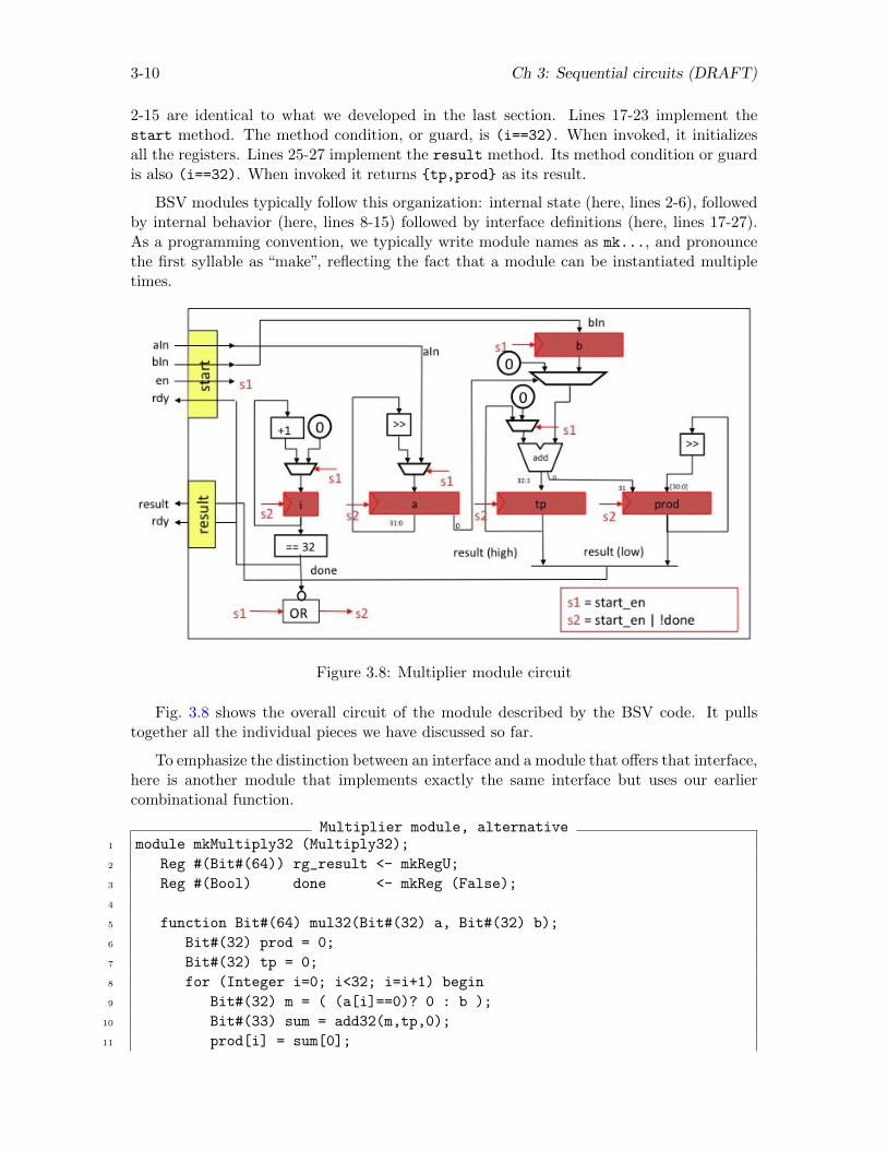
Figure 3.8: Multiplier module circuit
Fig. 3.8 shows the overall circuit of the module described by the BSV code. It pullstogether all the individual pieces we have discussed so far.
To emphasize the distinction between an interface and a module that offers that interface,here is another module that implements exactly the same interface but uses our earliercombinational function.
Multiplier module, alternative1 module mkMultiply32 (Multiply32);
2 Reg #(Bit#(64)) rg_result <- mkRegU;
3 Reg #(Bool) done <- mkReg (False);
4
5 function Bit#(64) mul32(Bit#(32) a, Bit#(32) b);
6 Bit#(32) prod = 0;
7 Bit#(32) tp = 0;
8 for (Integer i=0; i<32; i=i+1) begin
9 Bit#(32) m = ( (a[i]==0)? 0 : b );
10 Bit#(33) sum = add32(m,tp,0);
11 prod[i] = sum[0];

c©2012-2013 Arvind, R.S.Nikhil, J.Emer and M.Vijayaraghavan; All Rights Reserved 3-11
12 tp = truncateLSB(sum);
13 end
14 return {tp,prod};
15 endfunction
16
17 method Action start(Bit#(32) aIn, Bit#(32) bIn) if (! done);
18 rg_result <= mult32 (aIn, bIn);
19 done <= True;
20 endmethod
21
22 method Bit#(64) result if (done);
23 return rg_result;
24 endmethod
25 endmodule
Lines 4-14 are the same combinational function we saw earlier. The start methodsimply invokes the combinational function on its arguments and stores the output in therg_result register. The result register simply returns the value in the register, when thecomputation is done.
Similarly, one can have many other implementations of the same multiplier interface,with different internal algorithms that offer various efficiency tradeoffs (area, power, latency,throughput):
Multiplier module, more alternatives1 module mkBlockMultiply (Multiply);
2 module mkBoothMultiply (Multiply);
3.4.1 Polymorphic multiply module
Let us now generalize our multiplier circuit so that it doesn’t just work with 32-bit argu-ments, producing a 64-bit result, but works with n-bit arguments and produces a 2n-bitresult. Thus, we could use the same module in other environments which may require, say,a 13-bit multiplier or a 24-bit multiplier. The interface declaration changes to the following:
Polymorphic multiplier module interface1 interface Multiply #(numeric type tn);
2 method Action start (Bit#(tn) a, Bit#(tn) b);
3 method Bit#(TAdd#(tn,tn)) result;
4 endinterface
And the module definition changes to the following:
Polymorphic multiplier module1 module mkMultiply (Multiply #(tn));
2 Integer n = valueOf (tn);
3
4 Reg #(Bit#(n)) a <- mkRegU;
3-12 Ch 3: Sequential circuits (DRAFT)
5 Reg #(Bit#(n)) b <- mkRegU;
6 Reg #(Bit#(n)) prod <- mkRegU;
7 Reg #(Bit#(n)) tp <- mkRegU;
8 Reg #(Bit#(TAdd#(1,TLog#(tn)))) i <- mkReg (fromInteger(n));
9
10 rule mulStep if (i<32);
11 Bit#(n) m = (a[0]==0)? 0 : b;
12 a <= a >> 1;
13 Bit#(Tadd#(tn,1)) sum = addN(m,tp,0);
14 prod <= { sum[0], prod [n-1:1] };
15 tp <= truncateLSB(sum);
16 i <= i + 1;
17 endrule
18
19 method Action start(Bit#(n) aIn, Bit#(n) bIn) if (i==fromInteger(n));
20 a <= aIn;
21 b <= bIn;
22 i <= 0;
23 tp <= 0;
24 prod <= 0;
25 endmethod
26
27 method Bit#(64) result if (i==fromInteger(n));
28 return {tp,prod};
29 endmethod
30 endmodule
Note the use of the pseudo-function valueOf to convert from an integer in the typedomain to an integer in the value domain; the use of the function fromInteger to convertfrom type Integer to type Bit#(...), and the use of type-domain operators like TAdd,TLog and so on to derive related numeric types.
3.5 Register files
Figure 3.9: A Register File with four 8-bit registers
c©2012-2013 Arvind, R.S.Nikhil, J.Emer and M.Vijayaraghavan; All Rights Reserved 3-13
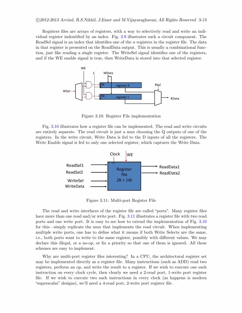
Registers files are arrays of registers, with a way to selectively read and write an indi-vidual register indentified by an index. Fig. 3.9 illustrates such a circuit component. TheReadSel signal is an index that identifies one of the n registers in the register file. The datain that register is presented on the ReadData output. This is usually a combinational func-tion, just like reading a single register. The WriteSel signal identifies one of the registers,and if the WE enable signal is true, then WriteData is stored into that selected register.
Figure 3.10: Register File implementation
Fig. 3.10 illustrates how a register file can be implemented. The read and write circuitsare entirely separate. The read circuit is just a mux choosing the Q outputs of one of theregisters. In the write circuit, Write Data is fed to the D inputs of all the registers. TheWrite Enable signal is fed to only one selected register, which captures the Write Data.
Figure 3.11: Multi-port Register File
The read and write interfaces of the register file are called “ports”. Many register fileshave more than one read and/or write port. Fig. 3.11 illustrates a register file with two readports and one write port. It is easy to see how to extend the implementation of Fig. 3.10for this—simply replicate the mux that implements the read circuit. When implementingmultiple write ports, one has to define what it means if both Write Selects are the same,i.e., both ports want to write to the same register, possibly with different values. We maydeclare this illegal, or a no-op, or fix a priority so that one of them is ignored. All theseschemes are easy to implement.
Why are multi-port register files interesting? In a CPU, the architectural register setmay be implemented directly as a register file. Many instructions (such as ADD) read tworegisters, perform an op, and write the result to a register. If we wish to execute one suchinstruction on every clock cycle, then clearly we need a 2-read port, 1-write port registerfile. If we wish to execute two such instructions in every clock (as happens is modern“superscalar” designs), we’ll need a 4-read port, 2-write port register file.
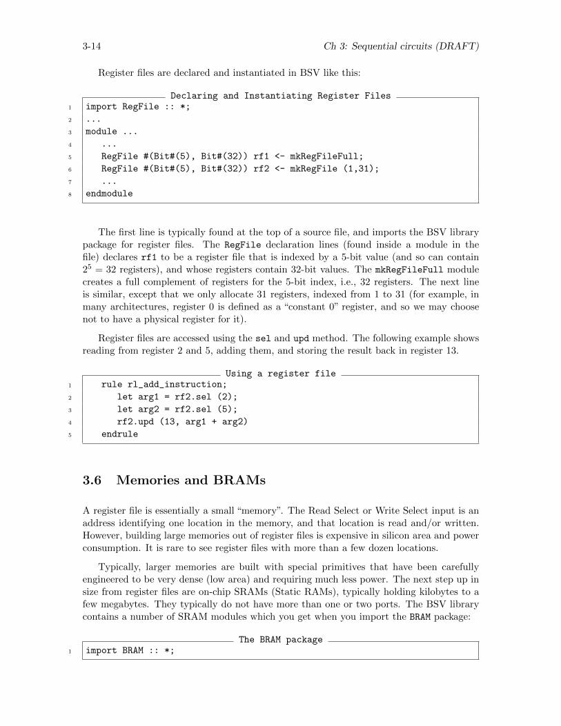
3-14 Ch 3: Sequential circuits (DRAFT)
Register files are declared and instantiated in BSV like this:
Declaring and Instantiating Register Files1 import RegFile :: *;
2 ...
3 module ...
4 ...
5 RegFile #(Bit#(5), Bit#(32)) rf1 <- mkRegFileFull;
6 RegFile #(Bit#(5), Bit#(32)) rf2 <- mkRegFile (1,31);
7 ...
8 endmodule
The first line is typically found at the top of a source file, and imports the BSV librarypackage for register files. The RegFile declaration lines (found inside a module in thefile) declares rf1 to be a register file that is indexed by a 5-bit value (and so can contain25 = 32 registers), and whose registers contain 32-bit values. The mkRegFileFull modulecreates a full complement of registers for the 5-bit index, i.e., 32 registers. The next lineis similar, except that we only allocate 31 registers, indexed from 1 to 31 (for example, inmany architectures, register 0 is defined as a “constant 0” register, and so we may choosenot to have a physical register for it).
Register files are accessed using the sel and upd method. The following example showsreading from register 2 and 5, adding them, and storing the result back in register 13.
Using a register file1 rule rl_add_instruction;
2 let arg1 = rf2.sel (2);
3 let arg2 = rf2.sel (5);
4 rf2.upd (13, arg1 + arg2)
5 endrule
3.6 Memories and BRAMs
A register file is essentially a small “memory”. The Read Select or Write Select input is anaddress identifying one location in the memory, and that location is read and/or written.However, building large memories out of register files is expensive in silicon area and powerconsumption. It is rare to see register files with more than a few dozen locations.
Typically, larger memories are built with special primitives that have been carefullyengineered to be very dense (low area) and requiring much less power. The next step up insize from register files are on-chip SRAMs (Static RAMs), typically holding kilobytes to afew megabytes. They typically do not have more than one or two ports. The BSV librarycontains a number of SRAM modules which you get when you import the BRAM package:
The BRAM package1 import BRAM :: *;
c©2012-2013 Arvind, R.S.Nikhil, J.Emer and M.Vijayaraghavan; All Rights Reserved 3-15
When you synthesize your BSV code for FPGAs, these will typically be “inferred” bydownstream FPGA synthesis tools as “Block RAMs” which are built-in high-density SRAMstructures on FPGAs. Whey you synthesize for ASICs, these will typically be “inferred” asSRAMs by downstream ASIC synthesis tools.
For even larger memories, you typically have to go to off-chip SRAMs (multi-megabytes)and DRAMs (Dynamic RAMs) in the megabyte to gigabyte range. On chip, you willtypically have a “memory interface” circuit that communicates with the off-chip memories.
Unlike register files, SRAMs and DRAMs usually do not have combinational reads, i.e.,data is only available 1 or more clock cycles after the address has been presented. And theytypically do not have multiple ports for reading or writing.

3-16 Ch 3: Sequential circuits (DRAFT)
Chapter 4
Pipelining Complex CombinationalCircuits
4.1 Introduction
In the last chapter we introduced sequential elements (registers), motivated by “folding”a large combinational circuit from an elaboration in space to an elaboration in time, inorder to reduce area. Let us now consider the throughput or repetition rate of such circuits.Suppose the circuit computes some function f() (e.g., multiply), and we wish repeatedly tocompute f() on a series of input datasets as fast as possible. The throughput of a circuitis measured by how often we can feed successive sets of inputs (which, in steady state, willbe the same as how often we can extract successive sets of outputs). Throughput is oftenexpressed in units such as as samples/second, megabits/second, etc., or by its inverse, therepetition rate, such as nanoseconds/sample.
In the pure combinational version (elaborated in space), we can feed the next set ofinputs to the circuit only after the current set has made it safely through the circuit, i.e.,after the longest combinational delay through the circuit. In practice what this means isthat the combinational circuit is likely to have registers at either end, and we will onlyclock these registers at a rate that ensures that signals have propagated safely through thecombinational circuit.
In the folded version (elaborated in time), after supplying one set of inputs we mustclock the circuit n times where n is the degree of folding, producing the final answer, beforewe supply the next set of inputs. The folded version can likely be clocked at much higherspeeds than the pure combinational version, since the largest combinational delay is likelyto be much smaller. However, the maximum throughput is likely to be somewhat less thanthe pure combinational version because, in both versions, each sample must flow throughthe same total amount of combinational logic before the next sample is accepted, and inthe folded version there is likely to some extra timing margin for safe registering in eachcirculation of data.
Note that in both the above versions, at any given time, the entire circuit is only involvedin computation for one set of inputs, i.e., the output must be delivered before we can acceptthe next set of inputs.
4-1
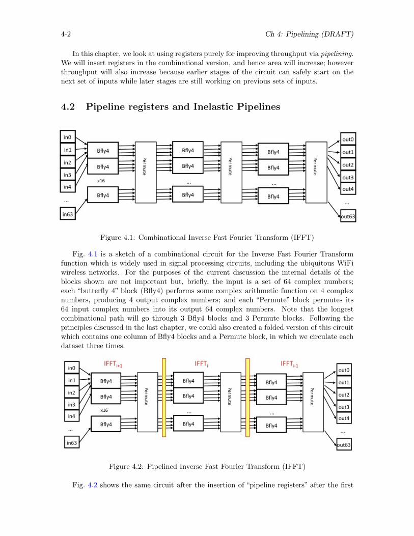
4-2 Ch 4: Pipelining (DRAFT)
In this chapter, we look at using registers purely for improving throughput via pipelining.We will insert registers in the combinational version, and hence area will increase; howeverthroughput will also increase because earlier stages of the circuit can safely start on thenext set of inputs while later stages are still working on previous sets of inputs.
4.2 Pipeline registers and Inelastic Pipelines
Figure 4.1: Combinational Inverse Fast Fourier Transform (IFFT)
Fig. 4.1 is a sketch of a combinational circuit for the Inverse Fast Fourier Transformfunction which is widely used in signal processing circuits, including the ubiquitous WiFiwireless networks. For the purposes of the current discussion the internal details of theblocks shown are not important but, briefly, the input is a set of 64 complex numbers;each “butterfly 4” block (Bfly4) performs some complex arithmetic function on 4 complexnumbers, producing 4 output complex numbers; and each “Permute” block permutes its64 input complex numbers into its output 64 complex numbers. Note that the longestcombinational path will go through 3 Bfly4 blocks and 3 Permute blocks. Following theprinciples discussed in the last chapter, we could also created a folded version of this circuitwhich contains one column of Bfly4 blocks and a Permute block, in which we circulate eachdataset three times.
Figure 4.2: Pipelined Inverse Fast Fourier Transform (IFFT)
Fig. 4.2 shows the same circuit after the insertion of “pipeline registers” after the first
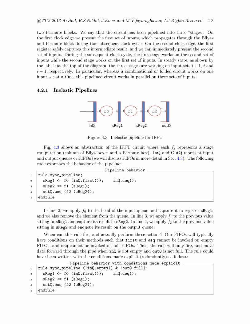
c©2012-2013 Arvind, R.S.Nikhil, J.Emer and M.Vijayaraghavan; All Rights Reserved 4-3
two Permute blocks. We say that the circuit has been pipelined into three “stages”. Onthe first clock edge we present the first set of inputs, which propagates through the Bfly4sand Permute block during the subsequent clock cycle. On the second clock edge, the firstregister safely captures this intermediate result, and we can immediately present the secondset of inputs. During the subsequent clock cycle, the first stage works on the second set ofinputs while the second stage works on the first set of inputs. In steady state, as shown bythe labels at the top of the diagram, the three stages are working on input sets i+ 1, i andi − 1, respectively. In particular, whereas a combinational or folded circuit works on oneinput set at a time, this pipelined circuit works in parallel on three sets of inputs.
4.2.1 Inelastic Pipelines
Figure 4.3: Inelastic pipeline for IFFT
Fig. 4.3 shows an abstraction of the IFFT circuit where each fj represents a stagecomputation (column of Bfly4 boxes and a Permute box). InQ and OutQ represent inputand output queues or FIFOs (we will discuss FIFOs in more detail in Sec. 4.3). The followingcode expresses the behavior of the pipeline:
Pipeline behavior1 rule sync_pipeline;
2 sReg1 <= f0 (inQ.first()); inQ.deq();
3 sReg2 <= f1 (sReg1);
4 outQ.enq (f2 (sReg2));
5 endrule
In line 2, we apply f0 to the head of the input queue and capture it in register sReg1;and we also remove the element from the queue. In line 3, we apply f1 to the previous valuesitting in sReg1 and capture its result in sReg2. In line 4, we apply f2 to the previous valuesitting in sReg2 and enqueue its result on the output queue.
When can this rule fire, and actually perform these actions? Our FIFOs will typicallyhave conditions on their methods such that first and deq cannot be invoked on emptyFIFOs, and enq cannot be invoked on full FIFOs. Thus, the rule will only fire, and movedata forward through the pipe when inQ is not empty and outQ is not full. The rule couldhave been written with the conditions made explicit (redundantly) as follows:
Pipeline behavior with conditions made explicit1 rule sync_pipeline (!inQ.empty() & !outQ.full);
2 sReg1 <= f0 (inQ.first()); inQ.deq();
3 sReg2 <= f1 (sReg1);
4 outQ.enq (f2 (sReg2));
5 endrule

4-4 Ch 4: Pipelining (DRAFT)
Recall that, semantically, all the actions in a rule occur simultaneously and instanta-neously. We also say that a rule is an atomic action or transaction. The code within arule should never be read as a sequential program. For example, there is no chance that,after dequeueing a dataset from inQ, we somehow then find that we are unable to enqueueinto outQ. Either the rule fires and everything in the rule happens, or it stalls and nothinghappens. As will become evident through the rest of the book, this is a key and pow-erful property for reasoning about the correctness of circuits. It is what fundamentallydistinguishes BSV from other hardware design languages.
4.2.2 Stalling and Bubbles
Suppose outQ is not full, but inQ is empty. The rule cannot fire, as just discussed, and wesay that the pipeline is stalled. Unfortunately, also, any data sitting in sReg1 and sReg2
will be stuck there until fresh input data arrive allowing the pipeline to move. We’ll nowmodify the rule to permit such data to continue moving. Once we do this, of course, wehave to distinguish the situation when a pipeline register actually contains data vs. it is“empty”. We do this by adding a flag bit to each pipeline register to indicate whether itcontains valid data or not, as illustrated in Fig. 4.4.
Figure 4.4: Valid bits on pipeline registers
When a pipeline register is empty, we also call this a bubble in the pipeline. The modifiedcode is shown below.
Adding Valid bits1 rule sync_pipeline;
2 if (inQ.notEmpty) begin
3 sReg1 <= f0 (inQ.first); inQ.deq;
4 sReg1f <= Valid
5 end
6 else
7 sReg1f <= Invalid;
8
9 sReg2 <= f1 (sReg1);
10 sReg2f <= sReg1f;
11
12 if (sReg2f == Valid)
13 outQ.enq (f2 (sReg2));
14 endrule
Lines 2-7 are the first stage: if inQ has data, we move the data as usual into sReg1,and also set sReg1f to the constant Valid. If inQ has no data, we set sReg1f to Invalid.
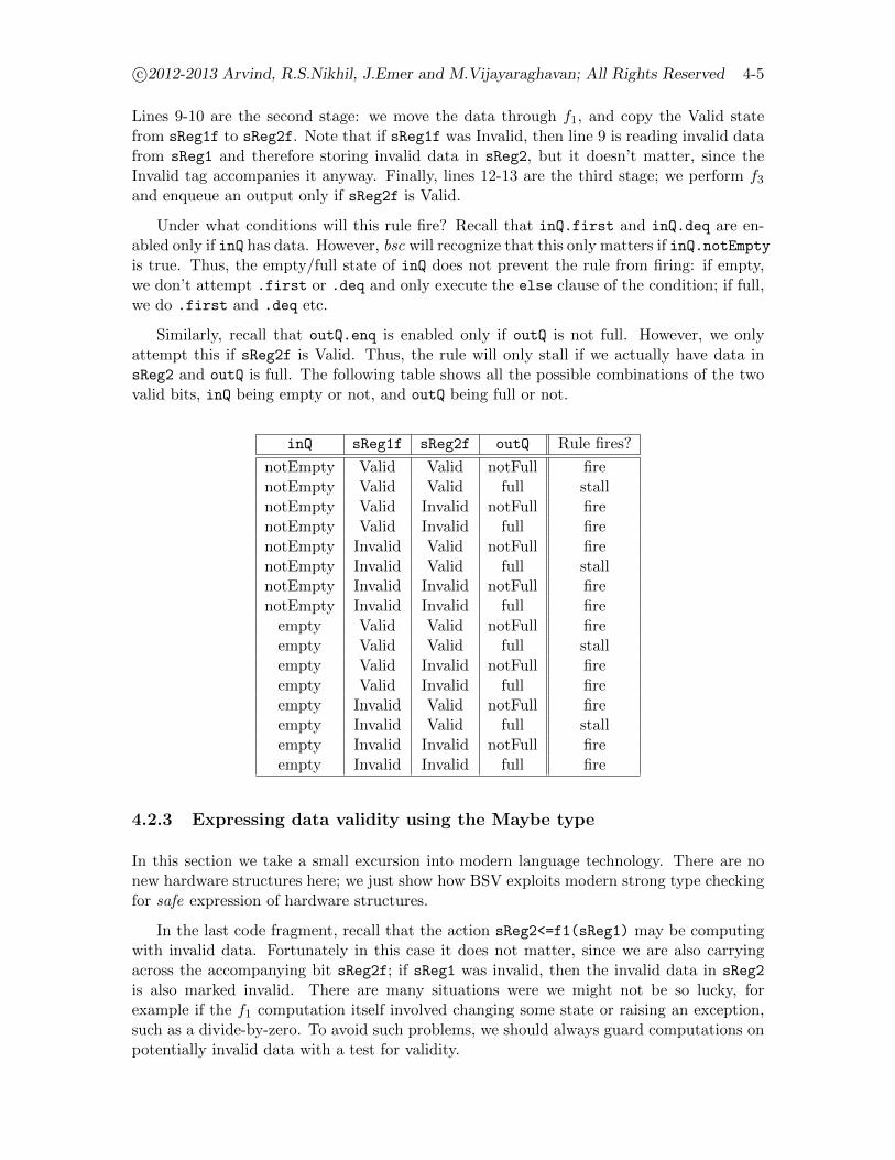
c©2012-2013 Arvind, R.S.Nikhil, J.Emer and M.Vijayaraghavan; All Rights Reserved 4-5
Lines 9-10 are the second stage: we move the data through f1, and copy the Valid statefrom sReg1f to sReg2f. Note that if sReg1f was Invalid, then line 9 is reading invalid datafrom sReg1 and therefore storing invalid data in sReg2, but it doesn’t matter, since theInvalid tag accompanies it anyway. Finally, lines 12-13 are the third stage; we perform f3and enqueue an output only if sReg2f is Valid.
Under what conditions will this rule fire? Recall that inQ.first and inQ.deq are en-abled only if inQ has data. However, bsc will recognize that this only matters if inQ.notEmptyis true. Thus, the empty/full state of inQ does not prevent the rule from firing: if empty,we don’t attempt .first or .deq and only execute the else clause of the condition; if full,we do .first and .deq etc.
Similarly, recall that outQ.enq is enabled only if outQ is not full. However, we onlyattempt this if sReg2f is Valid. Thus, the rule will only stall if we actually have data insReg2 and outQ is full. The following table shows all the possible combinations of the twovalid bits, inQ being empty or not, and outQ being full or not.
inQ sReg1f sReg2f outQ Rule fires?
notEmpty Valid Valid notFull firenotEmpty Valid Valid full stallnotEmpty Valid Invalid notFull firenotEmpty Valid Invalid full firenotEmpty Invalid Valid notFull firenotEmpty Invalid Valid full stallnotEmpty Invalid Invalid notFull firenotEmpty Invalid Invalid full fire
empty Valid Valid notFull fireempty Valid Valid full stallempty Valid Invalid notFull fireempty Valid Invalid full fireempty Invalid Valid notFull fireempty Invalid Valid full stallempty Invalid Invalid notFull fireempty Invalid Invalid full fire
4.2.3 Expressing data validity using the Maybe type
In this section we take a small excursion into modern language technology. There are nonew hardware structures here; we just show how BSV exploits modern strong type checkingfor safe expression of hardware structures.
In the last code fragment, recall that the action sReg2<=f1(sReg1) may be computingwith invalid data. Fortunately in this case it does not matter, since we are also carryingacross the accompanying bit sReg2f; if sReg1 was invalid, then the invalid data in sReg2
is also marked invalid. There are many situations were we might not be so lucky, forexample if the f1 computation itself involved changing some state or raising an exception,such as a divide-by-zero. To avoid such problems, we should always guard computations onpotentially invalid data with a test for validity.
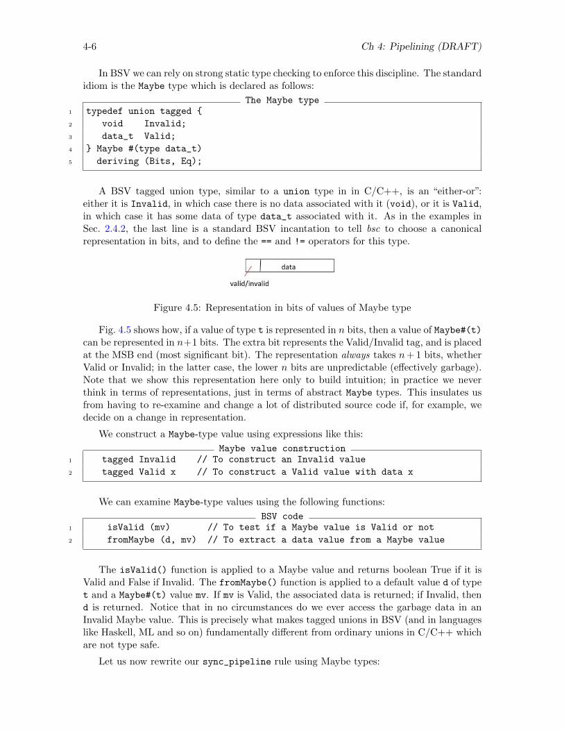
4-6 Ch 4: Pipelining (DRAFT)
In BSV we can rely on strong static type checking to enforce this discipline. The standardidiom is the Maybe type which is declared as follows:
The Maybe type1 typedef union tagged {
2 void Invalid;
3 data_t Valid;
4 } Maybe #(type data_t)
5 deriving (Bits, Eq);
A BSV tagged union type, similar to a union type in in C/C++, is an “either-or”:either it is Invalid, in which case there is no data associated with it (void), or it is Valid,in which case it has some data of type data_t associated with it. As in the examples inSec. 2.4.2, the last line is a standard BSV incantation to tell bsc to choose a canonicalrepresentation in bits, and to define the == and != operators for this type.
Figure 4.5: Representation in bits of values of Maybe type
Fig. 4.5 shows how, if a value of type t is represented in n bits, then a value of Maybe#(t)can be represented in n+1 bits. The extra bit represents the Valid/Invalid tag, and is placedat the MSB end (most significant bit). The representation always takes n+ 1 bits, whetherValid or Invalid; in the latter case, the lower n bits are unpredictable (effectively garbage).Note that we show this representation here only to build intuition; in practice we neverthink in terms of representations, just in terms of abstract Maybe types. This insulates usfrom having to re-examine and change a lot of distributed source code if, for example, wedecide on a change in representation.
We construct a Maybe-type value using expressions like this:
Maybe value construction1 tagged Invalid // To construct an Invalid value
2 tagged Valid x // To construct a Valid value with data x
We can examine Maybe-type values using the following functions:
BSV code1 isValid (mv) // To test if a Maybe value is Valid or not
2 fromMaybe (d, mv) // To extract a data value from a Maybe value
The isValid() function is applied to a Maybe value and returns boolean True if it isValid and False if Invalid. The fromMaybe() function is applied to a default value d of typet and a Maybe#(t) value mv. If mv is Valid, the associated data is returned; if Invalid, thend is returned. Notice that in no circumstances do we ever access the garbage data in anInvalid Maybe value. This is precisely what makes tagged unions in BSV (and in languageslike Haskell, ML and so on) fundamentally different from ordinary unions in C/C++ whichare not type safe.
Let us now rewrite our sync_pipeline rule using Maybe types:
c©2012-2013 Arvind, R.S.Nikhil, J.Emer and M.Vijayaraghavan; All Rights Reserved 4-7
Using Maybe types1 module ...
2 ...
3 Reg #(Maybe #(t)) sReg1 <- mkRegU;
4 Reg #(Maybe #(t)) sReg2 <- mkRegU;
5
6 rule sync_pipeline;
7 if (inQ.notEmpty)
8 sReg1 <= tagged Valid (f0 (inQ.first)); inQ.deq;
9 else
10 sReg1 <= tagged Invalid;
11
12 sReg2 <= ( isValid (sReg1) ? tagged Valid f1 (fromMaybe (?, sReg1))
13 : tagged Invalid );
14
15 if (isValid (sReg2))
16 outQ.enq (f2 (fromMaybe (?, sReg2)));
17 endrule
18 ...
19 endmodule
In lines 3-4 we declare sReg1 and sReg2 now to contain Maybe values. In lines 8 and 10we construct Valid and Invalid values, respectively. In lines 12-13 we test sReg1 for validity,and we construct Valid and Invalid values for sReg2, respectively. We supply a “don’t care”argument (?) to fromMaybe because we have guarded this with a test for validity. Finally,in lines 15-16 we test sReg2 for validity, and use fromMaybe again to extract its value.
Instead of using the functions isValid and fromMaybe, tagged unions are more oftenexamined using the much more readable “pattern matching” notation:
Using Maybe types1 rule sync_pipeline;
2 if (inQ.notEmpty)
3 sReg1 <= tagged Valid (f0 (inQ.first)); inQ.deq;
4 else
5 sReg1 <= tagged Invalid;
6
7 case (sReg1) matches
8 tagged Invalid : sReg2 <= tagged Invalid;
9 tagged Valid .x: sReg2 <= tagged Valid f1 (x);
10 endcase
11
12 case (sReg2) matches
13 tagged Valid .x: outQ.enq (f2 (x));
14 endcase
15 endrule
Notice the keyword matches in the case statements. In each clause of the case state-ments, the left-hand side (before the “:”) is a pattern to match against the Maybe value. In

4-8 Ch 4: Pipelining (DRAFT)
line 9, the pattern tagged Valid .x not only checks if sReg1 is a valid value, but it alsobinds the new variable x to the contained data; this is used in the right-hand side as anargument to f1. Note the dot “.” in front of the x in the pattern: this signals that x is a newpattern variable that is effectively declared at this point, and must be bound to whatever isin the value in that position (its type is obvious, and inferred, based on its position in thepattern). The scope of x is the right-hand side of that case clause.
4.3 Elastic Pipelines with FIFOs between stages
In inelastic pipelines (previous section) each stage is separated by an ordinary register,and the overall behavior is expressed in a rule the combines the behavior of each stageinto a single atomic (and therefore synchronous) transaction. In elastic pipelines, eachstage is separated by a FIFO, and each stage’s behavior is expressed as rule that may fireindependently (asynchronously) with respect to the other stages.
Figure 4.6: An elastic pipeline
Fig. 4.6 shows a sketch of an elastic pipeline. The BSV code structure is shown below:
Elastic pipeline1 import FIFOF :: *;
2
3 module ...
4 ...
5 FIFOF #(t) inQ <- mkFIFOF;
6 FIFOF #(t) fifo1 <- mkFIFOF;
7 FIFOF #(t) fifo2 <- mkFIFOF;
8 FIFOF #(t) outQ <- mkFIFOF;
9
10 rule stage1;
11 fifo1.enq (f1 (inQ.first); inQ.deq;
12 endrule
13
14 rule stage2;
15 fifo2.enq (f2 (fifo1.first); fifo1.deq();
16 endrule
17
18 rule stage3;
19 outQ.enq (f3 (fifo2.first); fifo2.deq;
20 endrule
21 ...
22 endmodule
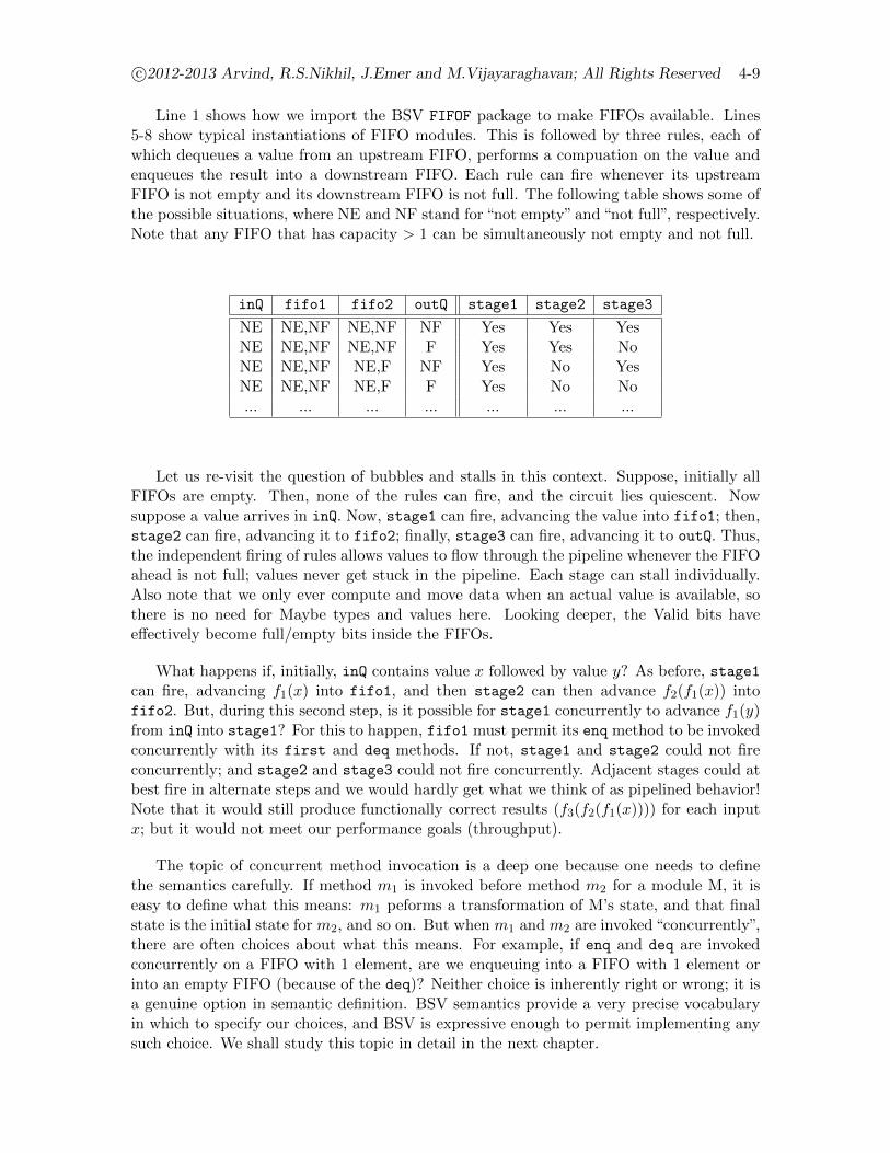
c©2012-2013 Arvind, R.S.Nikhil, J.Emer and M.Vijayaraghavan; All Rights Reserved 4-9
Line 1 shows how we import the BSV FIFOF package to make FIFOs available. Lines5-8 show typical instantiations of FIFO modules. This is followed by three rules, each ofwhich dequeues a value from an upstream FIFO, performs a compuation on the value andenqueues the result into a downstream FIFO. Each rule can fire whenever its upstreamFIFO is not empty and its downstream FIFO is not full. The following table shows some ofthe possible situations, where NE and NF stand for “not empty” and “not full”, respectively.Note that any FIFO that has capacity > 1 can be simultaneously not empty and not full.
inQ fifo1 fifo2 outQ stage1 stage2 stage3
NE NE,NF NE,NF NF Yes Yes YesNE NE,NF NE,NF F Yes Yes NoNE NE,NF NE,F NF Yes No YesNE NE,NF NE,F F Yes No No... ... ... ... ... ... ...
Let us re-visit the question of bubbles and stalls in this context. Suppose, initially allFIFOs are empty. Then, none of the rules can fire, and the circuit lies quiescent. Nowsuppose a value arrives in inQ. Now, stage1 can fire, advancing the value into fifo1; then,stage2 can fire, advancing it to fifo2; finally, stage3 can fire, advancing it to outQ. Thus,the independent firing of rules allows values to flow through the pipeline whenever the FIFOahead is not full; values never get stuck in the pipeline. Each stage can stall individually.Also note that we only ever compute and move data when an actual value is available, sothere is no need for Maybe types and values here. Looking deeper, the Valid bits haveeffectively become full/empty bits inside the FIFOs.
What happens if, initially, inQ contains value x followed by value y? As before, stage1can fire, advancing f1(x) into fifo1, and then stage2 can then advance f2(f1(x)) intofifo2. But, during this second step, is it possible for stage1 concurrently to advance f1(y)from inQ into stage1? For this to happen, fifo1 must permit its enq method to be invokedconcurrently with its first and deq methods. If not, stage1 and stage2 could not fireconcurrently; and stage2 and stage3 could not fire concurrently. Adjacent stages could atbest fire in alternate steps and we would hardly get what we think of as pipelined behavior!Note that it would still produce functionally correct results (f3(f2(f1(x)))) for each inputx; but it would not meet our performance goals (throughput).
The topic of concurrent method invocation is a deep one because one needs to definethe semantics carefully. If method m1 is invoked before method m2 for a module M, it iseasy to define what this means: m1 peforms a transformation of M’s state, and that finalstate is the initial state for m2, and so on. But when m1 and m2 are invoked “concurrently”,there are often choices about what this means. For example, if enq and deq are invokedconcurrently on a FIFO with 1 element, are we enqueuing into a FIFO with 1 element orinto an empty FIFO (because of the deq)? Neither choice is inherently right or wrong; it isa genuine option in semantic definition. BSV semantics provide a very precise vocabularyin which to specify our choices, and BSV is expressive enough to permit implementing anysuch choice. We shall study this topic in detail in the next chapter.
4-10 Ch 4: Pipelining (DRAFT)
4.4 Final comments on Inelastic and Elastic Pipelines
Inelastic pipeline stages are typically separated by ordinary registers, and behavior (datamovement) is expressed as a single rule that specifies the actions of all the stages. All theactions happen as a single, atomic transaction. We saw that, in order to handle pipelinebubbles and keep data moving, we had to introduce a lot of “flow control” control logic:valid bits to accompany data, and many conditionals in the rule to manage data movement.It was not trivial to reason about correctness, i.e., that our circuit did not accidentally dropa valid sample or overwrite one with another. The problem with writing pipelines in thisstyle (which is the natural style in Verilog and VHDL) is that it does not evolve or scaleeasily; it gets more and more complex with each change, and as we go to larger pipelines.For scalability one would like a compositional way to define pipelines, where we define stagesindividually and then compose them into pipelines.
Elastic pipeline stages are typically separated by FIFOs, and each stage’s behavior isexpressed as an individual, local rule. Flow control is naturally encapsulated into methodconditions preventing us from enqueuing into a full FIFO and from dequeuing from anempty FIFO. Correctness is more obvious in such pipelines, and they are easier to write ina compositional (modular) way. However, when we compose elastic descriptions into largersystems, we must ensure that rules can fire concurrently when they have to, so that weachieve our desired throughput.

Chapter 5
Introduction to SMIPS: a basicimplementation without pipelining
5.1 Introduction to SMIPS
We now have enough foundational material to turn to the central focus of this book, namely,processor architectures. An immediate choice is: which instruction set? We can invent anew one, or reuse an existing instruction set. The advantages of the latter include validationand credibility (it has been tested in the the field and in commercial products). More impor-tantly, we can reuse existing tool chains (compilers, linkers, debuggers) and system software(operating systems, device drivers) in order quickly to produce realistic programs to run onour system. Real system software and applications are essential for taking meaningful andcredible measurements regarding efficiency and performance of hardware implementations.
In this book, we will be implementing an instruction set architecture (ISA) called SMIPS(“Simple MIPS”), which is a subset of the full MIPS32 ISA. MIPS was one of the firstcommercial RISC (Reduced Instruction Set Computer) processors and continues to be usedin a wide range of commercial products such as Casio PDAs, Sony Playstation and Ciscointernet routers (see Appendix A for some more history). MIPS implementations probablyspan the widest range for any commercial ISA, from simple single-issue in-order pipelinesto quad-issue out-of-order superscalar processors.
Our subset, SMIPS, does not include floating point instructions, trap instructions, mis-aligned load/stores, branch and link instructions, or branch likely instructions. There arethree SMIPS variants which are discussed in more detail in Appendix A. SMIPSv1 has onlyfive instructions and it is mainly used as a toy ISA for instructional purposes. SMIPSv2includes the basic integer, memory, and control instructions. It excludes multiply instruc-tions, divide instructions, byte/halfword loads/stores, and instructions which cause arith-metic overflows. Neither SMIPSv1 noor SMIPSv2 support exceptions, interrupts, or mostof the system coprocessor. SMIPSv3 is the full SMIPS ISA and includes all the instructionsin our MIPS subset.
Appendix A has a detailed technical reference for SMIPS. We now sketch a high-leveloverview.
5-1
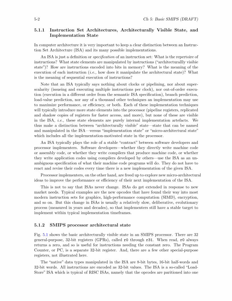
5-2 Ch 5: Basic SMIPS (DRAFT)
5.1.1 Instruction Set Architectures, Architecturally Visible State, andImplementation State
In computer architecture it is very important to keep a clear distinction between an Instruc-tion Set Architecture (ISA) and its many possible implementations.
An ISA is just a definition or specification of an instruction set: What is the repertoire ofinstructions? What state elements are manipulated by instructions (“architecturallly visibiestate”)? How are instructions encoded into bits in memory? What is the meaning of theexecution of each instruction (i.e., how does it manipulate the architectural state)? Whatis the meaning of sequential execution of instructions?
Note that an ISA typically says nothing about clocks or pipelining, nor about super-scalarity (issueing and executing multiple instructions per clock), nor out-of-order execu-tion (execution in a different order from the semantic ISA specification), branch prediction,load-value prediction, nor any of a thousand other techniques an implementation may useto maximize performance, or efficiency, or both. Each of these implementation techniqueswill typically introduce more state elements into the processor (pipeline registers, replicatedand shadow copies of registers for faster access, and more), but none of these are visiblein the ISA, i.e., these state elements are purely internal implementation artefacts. Wethus make a distinction between “architecturally visible” state—state that can be namedand manipulated in the ISA—versus “implementation state” or “micro-architectural state”which includes all the implementation-motivated state in the processor.
An ISA typically plays the role of a stable “contract” between software developers andprocessor implementers. Software developers—whether they directly write machine codeor assembly code, or whether they write compilers that produce machine code, or whetherthey write application codes using compilers developed by others—use the ISA as an un-ambiguous specification of what their machine code programs will do. They do not have toreact and revise their codes every time there is a new implementation of the given ISA.
Processor implementers, on the other hand, are freed up to explore new micro-architecturalideas to improve the performance or efficiency of their next implementation of the ISA.
This is not to say that ISAs never change. ISAs do get extended in response to newmarket needs. Typical examples are the new opcodes that have found their way into mostmodern instruction sets for graphics, high-performance computation (SIMD), encryption,and so on. But this change in ISAs is usually a relatively slow, deliberative, evolutionaryprocess (measured in years and decades), so that implementers still have a stable target toimplement within typical implementation timeframes.
5.1.2 SMIPS processor architectural state
Fig. 5.1 shows the basic architecturally visible state in an SMIPS processor. There are 32general-purpose, 32-bit registers (GPRs), called r0 through r31. When read, r0 alwaysreturns a zero, and so is useful for instructions needing the constant zero. The ProgramCounter, or PC, is a separate 32-bit register. And, there are a few other special-purposeregisters, not illustrated here.
The “native” data types manipulated in the ISA are 8-bit bytes, 16-bit half-words and32-bit words. All instructions are encoded as 32-bit values. The ISA is a so-called “Load-Store” ISA which is typical of RISC ISAs, namely that the opcodes are paritioned into one
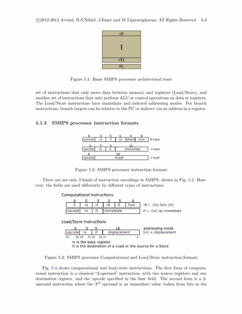
c©2012-2013 Arvind, R.S.Nikhil, J.Emer and M.Vijayaraghavan; All Rights Reserved 5-3
Figure 5.1: Basic SMIPS processor architectural state
set of instructions that only move data between memory and registers (Load/Store), andanother set of instructions that only perform ALU or control operations on data in registers.The Load/Store instructions have immediate and indexed addressing modes. For branchinstructions, branch targets can be relative to the PC or indirect via an address in a register.
5.1.3 SMIPS processor instruction formats
Figure 5.2: SMIPS processor instruction formats
There are are only 3 kinds of instruction encodings in SMIPS, shown in Fig. 5.2. How-ever, the fields are used differently by different types of instructions.
Figure 5.3: SMIPS processor Computational and Load/Store instruction formats
Fig. 5.3 shows computational and load/store instructions. The first form of computa-tional instruction is a classical “3-operand” instruction, with two source registers and onedestination register, and the opcode specified in the func field. The second form is a 2-operand instruction where the 3rd operand is an immediate value (taken from bits in the
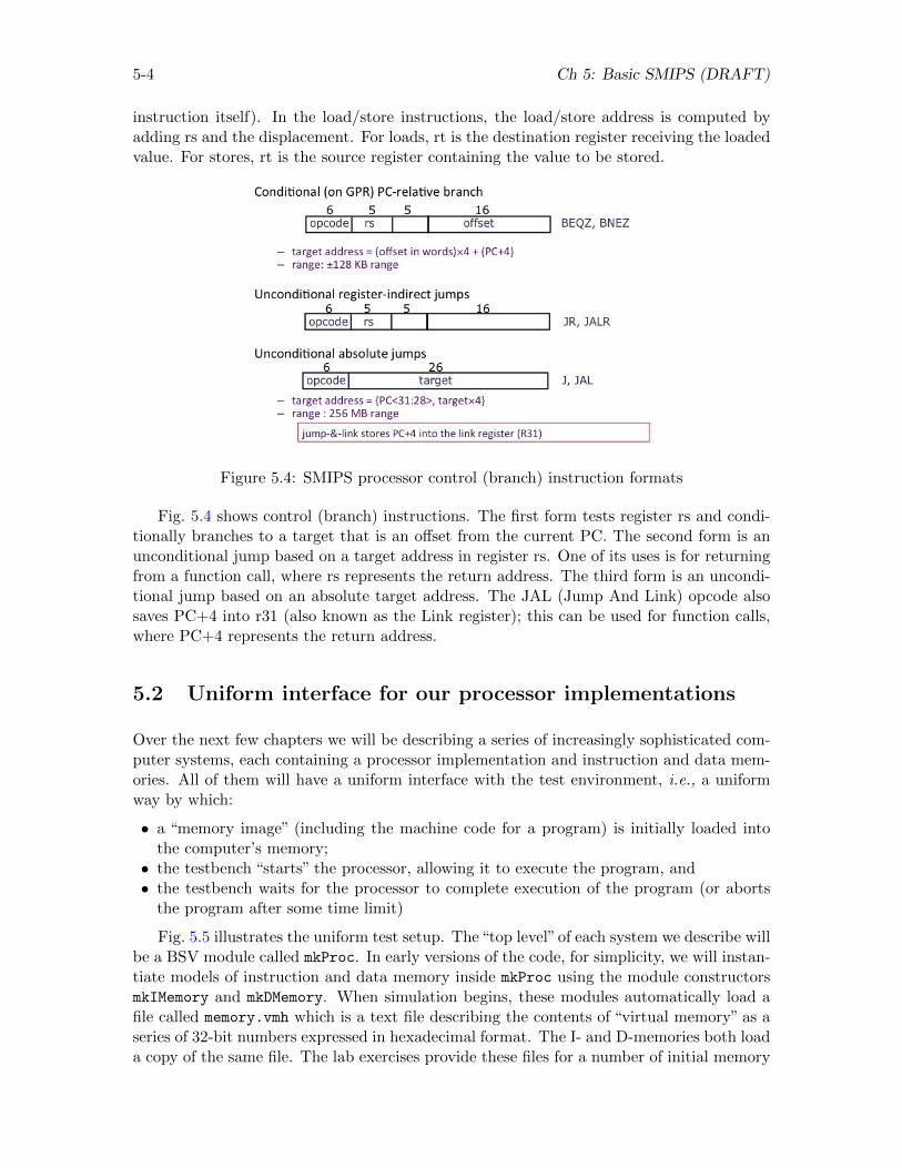
5-4 Ch 5: Basic SMIPS (DRAFT)
instruction itself). In the load/store instructions, the load/store address is computed byadding rs and the displacement. For loads, rt is the destination register receiving the loadedvalue. For stores, rt is the source register containing the value to be stored.
Figure 5.4: SMIPS processor control (branch) instruction formats
Fig. 5.4 shows control (branch) instructions. The first form tests register rs and condi-tionally branches to a target that is an offset from the current PC. The second form is anunconditional jump based on a target address in register rs. One of its uses is for returningfrom a function call, where rs represents the return address. The third form is an uncondi-tional jump based on an absolute target address. The JAL (Jump And Link) opcode alsosaves PC+4 into r31 (also known as the Link register); this can be used for function calls,where PC+4 represents the return address.
5.2 Uniform interface for our processor implementations
Over the next few chapters we will be describing a series of increasingly sophisticated com-puter systems, each containing a processor implementation and instruction and data mem-ories. All of them will have a uniform interface with the test environment, i.e., a uniformway by which:
• a “memory image” (including the machine code for a program) is initially loaded intothe computer’s memory;
• the testbench “starts” the processor, allowing it to execute the program, and• the testbench waits for the processor to complete execution of the program (or aborts
the program after some time limit)
Fig. 5.5 illustrates the uniform test setup. The“top level”of each system we describe willbe a BSV module called mkProc. In early versions of the code, for simplicity, we will instan-tiate models of instruction and data memory inside mkProc using the module constructorsmkIMemory and mkDMemory. When simulation begins, these modules automatically load afile called memory.vmh which is a text file describing the contents of “virtual memory” as aseries of 32-bit numbers expressed in hexadecimal format. The I- and D-memories both loada copy of the same file. The lab exercises provide these files for a number of initial memory
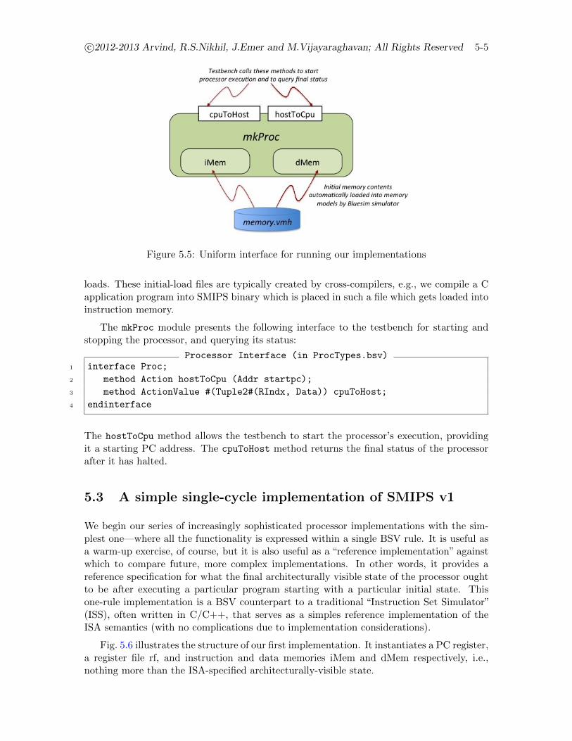
c©2012-2013 Arvind, R.S.Nikhil, J.Emer and M.Vijayaraghavan; All Rights Reserved 5-5
Figure 5.5: Uniform interface for running our implementations
loads. These initial-load files are typically created by cross-compilers, e.g., we compile a Capplication program into SMIPS binary which is placed in such a file which gets loaded intoinstruction memory.
The mkProc module presents the following interface to the testbench for starting andstopping the processor, and querying its status:
Processor Interface (in ProcTypes.bsv)1 interface Proc;
2 method Action hostToCpu (Addr startpc);
3 method ActionValue #(Tuple2#(RIndx, Data)) cpuToHost;
4 endinterface
The hostToCpu method allows the testbench to start the processor’s execution, providingit a starting PC address. The cpuToHost method returns the final status of the processorafter it has halted.
5.3 A simple single-cycle implementation of SMIPS v1
We begin our series of increasingly sophisticated processor implementations with the sim-plest one—where all the functionality is expressed within a single BSV rule. It is useful asa warm-up exercise, of course, but it is also useful as a “reference implementation” againstwhich to compare future, more complex implementations. In other words, it provides areference specification for what the final architecturally visible state of the processor oughtto be after executing a particular program starting with a particular initial state. Thisone-rule implementation is a BSV counterpart to a traditional “Instruction Set Simulator”(ISS), often written in C/C++, that serves as a simples reference implementation of theISA semantics (with no complications due to implementation considerations).
Fig. 5.6 illustrates the structure of our first implementation. It instantiates a PC register,a register file rf, and instruction and data memories iMem and dMem respectively, i.e.,nothing more than the ISA-specified architecturally-visible state.
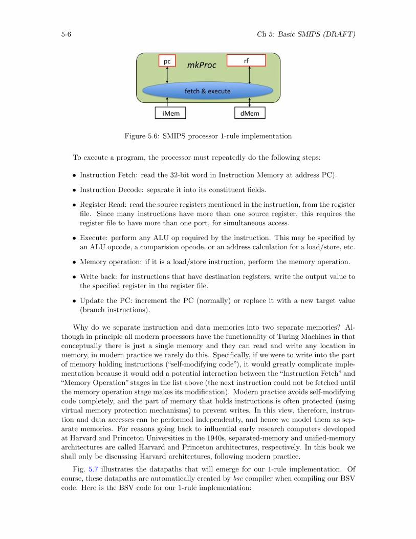
5-6 Ch 5: Basic SMIPS (DRAFT)
Figure 5.6: SMIPS processor 1-rule implementation
To execute a program, the processor must repeatedly do the following steps:
• Instruction Fetch: read the 32-bit word in Instruction Memory at address PC).
• Instruction Decode: separate it into its constituent fields.
• Register Read: read the source registers mentioned in the instruction, from the registerfile. Since many instructions have more than one source register, this requires theregister file to have more than one port, for simultaneous access.
• Execute: perform any ALU op required by the instruction. This may be specified byan ALU opcode, a comparision opcode, or an address calculation for a load/store, etc.
• Memory operation: if it is a load/store instruction, perform the memory operation.
• Write back: for instructions that have destination registers, write the output value tothe specified register in the register file.
• Update the PC: increment the PC (normally) or replace it with a new target value(branch instructions).
Why do we separate instruction and data memories into two separate memories? Al-though in principle all modern processors have the functionality of Turing Machines in thatconceptually there is just a single memory and they can read and write any location inmemory, in modern practice we rarely do this. Specifically, if we were to write into the partof memory holding instructions (“self-modifying code”), it would greatly complicate imple-mentation because it would add a potential interaction between the “Instruction Fetch” and“Memory Operation” stages in the list above (the next instruction could not be fetched untilthe memory operation stage makes its modification). Modern practice avoids self-modifyingcode completely, and the part of memory that holds instructions is often protected (usingvirtual memory protection mechanisms) to prevent writes. In this view, therefore, instruc-tion and data accesses can be performed independently, and hence we model them as sep-arate memories. For reasons going back to influential early research computers developedat Harvard and Princeton Universities in the 1940s, separated-memory and unified-memoryarchitectures are called Harvard and Princeton architectures, respectively. In this book weshall only be discussing Harvard architectures, following modern practice.
Fig. 5.7 illustrates the datapaths that will emerge for our 1-rule implementation. Ofcourse, these datapaths are automatically created by bsc compiler when compiling our BSVcode. Here is the BSV code for our 1-rule implementation:
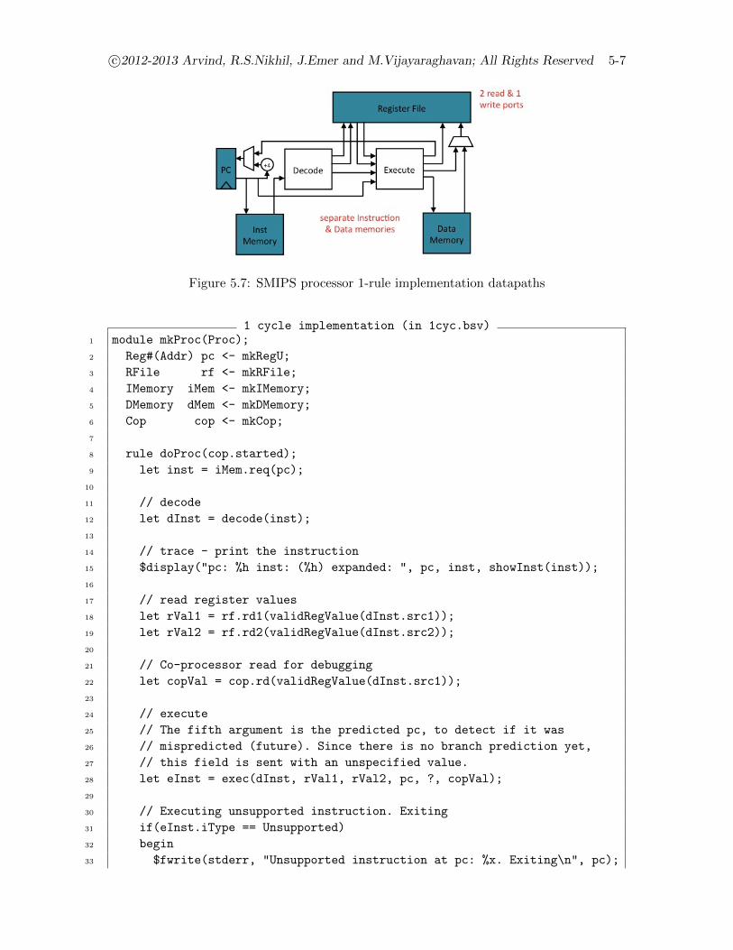
c©2012-2013 Arvind, R.S.Nikhil, J.Emer and M.Vijayaraghavan; All Rights Reserved 5-7
Figure 5.7: SMIPS processor 1-rule implementation datapaths
1 cycle implementation (in 1cyc.bsv)1 module mkProc(Proc);
2 Reg#(Addr) pc <- mkRegU;
3 RFile rf <- mkRFile;
4 IMemory iMem <- mkIMemory;
5 DMemory dMem <- mkDMemory;
6 Cop cop <- mkCop;
7
8 rule doProc(cop.started);
9 let inst = iMem.req(pc);
10
11 // decode
12 let dInst = decode(inst);
13
14 // trace - print the instruction
15 $display("pc: %h inst: (%h) expanded: ", pc, inst, showInst(inst));
16
17 // read register values
18 let rVal1 = rf.rd1(validRegValue(dInst.src1));
19 let rVal2 = rf.rd2(validRegValue(dInst.src2));
20
21 // Co-processor read for debugging
22 let copVal = cop.rd(validRegValue(dInst.src1));
23
24 // execute
25 // The fifth argument is the predicted pc, to detect if it was
26 // mispredicted (future). Since there is no branch prediction yet,
27 // this field is sent with an unspecified value.
28 let eInst = exec(dInst, rVal1, rVal2, pc, ?, copVal);
29
30 // Executing unsupported instruction. Exiting
31 if(eInst.iType == Unsupported)
32 begin
33 $fwrite(stderr, "Unsupported instruction at pc: %x. Exiting\n", pc);
5-8 Ch 5: Basic SMIPS (DRAFT)
34 $finish;
35 end
36
37 // memory
38 if(eInst.iType == Ld) begin
39 eInst.data <- dMem.req(MemReq{op: Ld, addr: eInst.addr, data: ?});
40 end
41 else if(eInst.iType == St) begin
42 let d <- dMem.req(MemReq{op: St, addr: eInst.addr, data: eInst.data});
43 end
44
45 // write back
46 if(isValid(eInst.dst) && validValue(eInst.dst).regType == Normal)
47 rf.wr(validRegValue(eInst.dst), eInst.data);
48
49 // update the pc depending on whether the branch is taken or not
50 pc <= eInst.brTaken ? eInst.addr : pc + 4;
51
52 // Co-processor write for debugging and stats
53 cop.wr(eInst.dst, eInst.data);
54 endrule
55
56 method ActionValue#(Tuple2#(RIndx, Data)) cpuToHost;
57 let ret <- cop.cpuToHost;
58 $display("sending %d %d", tpl_1(ret), tpl_2(ret));
59 return ret;
60 endmethod
61
62 method Action hostToCpu(Bit#(32) startpc) if (!cop.started);
63 cop.start;
64 pc <= startpc;
65 endmethod
66 endmodule
Line 2 declares the mkProc module with the previously described Proc interface. Lines3-7 instantiate the sub-modules: the PC register, a register file, the instruction and datamemories, and cop, a standard co-processor. The co-processor is the administrative con-troller of the processor, allowing it to start, stop, keeping a record of time (cycle count),number of instructions executed, and so on.
Lines 9-54 specify the single rule that does everything, and it is only enabled whencop.started is true. It more-or-less follows the itemized list described earlier: Line 10 isthe Instruction Fetch; line 13 is Instruction Decode. Lines 19-20 perform the two sourceregister reads (the validRegValue functions are needed because not all instructions havetwo source registers). Ignore line 23 for now; it’s using the co-processor for debugging. Line28 is Execute. Lines 30-35 detect bad instructions (not supported in this ISA). Lines 37-43do the memory operation, if any. Line 46-47 do the Write Back, if any, and line 50 updatesthe PC. Lines 56-65 implement the Proc interface methods.
c©2012-2013 Arvind, R.S.Nikhil, J.Emer and M.Vijayaraghavan; All Rights Reserved 5-9
Note that all the functions and methods used in this rule including iMem.req(), decode(),rf.rd1(), rf.rd2(), exec(), dMem.req(), and rf.wr() are instantaneous (purely combi-national). In fact they must be, since they are in a single rule.
Let us dig a little deeper into the BSV code. We start with some type definitions:
Some type definitions (in ProcTypes.bsv)1 typedef Bit#(5) RIndx;
2
3 typedef enum {Unsupported, Alu, Ld, St, J, Jr, Br, Mfc0, Mtc0} IType
4 deriving(Bits, Eq);
5 typedef enum {Eq, Neq, Le, Lt, Ge, Gt, AT, NT} BrFunc
6 deriving(Bits, Eq);
7 typedef enum {Add, Sub, And, Or, Xor, Nor,
8 Slt, Sltu, LShift, RShift, Sra} AluFunc
9 deriving(Bits, Eq);
Line 1 defines a register index to be a 5-bit value (since we have 32 registers in SMIPS).The next few lines describe symbolic names for various opcode functions. The followingcode describes a decoded instruction:
Decoded instructions (in ProcTypes.bsv)1 typedef struct {
2 IType iType;
3 AluFunc aluFunc;
4 BrFunc brFunc;
5 Maybe#(FullIndx) dst;
6 Maybe#(FullIndx) src1;
7 Maybe#(FullIndx) src2;
8 Maybe#(Data) imm;
9 } DecodedInst deriving(Bits, Eq);
The decode() function is in the file Decode.bsv and has the following outline:
Decode function outline (in Decode.bsv)1 function DecodedInst decode(Data inst);
2 DecodedInst dInst = ?;
3 let opcode = inst[ 31 : 26 ];
4 let rs = inst[ 25 : 21 ];
5 let rt = inst[ 20 : 16 ];
6 let rd = inst[ 15 : 11 ];
7 let shamt = inst[ 10 : 6 ];
8 let funct = inst[ 5 : 0 ];
9 let imm = inst[ 15 : 0 ];
10 let target = inst[ 25 : 0 ];
11
12 case (opcode)
13 ... fill out the dInst structure accordingly ...
14 endcase
5-10 Ch 5: Basic SMIPS (DRAFT)
15 return dInst;
16 endfunction
We show below one of the case arms, corresponding to I-Type ALU instructions:
Decode function; I-type section (in Decode.bsv)1 ...
2 case (opcode)
3 opADDIU, opSLTI, opSLTIU, opANDI, opORI, opXORI, opLUI:
4 begin
5 dInst.iType = Alu;
6 dInst.aluFunc = case (opcode)
7 opADDIU, opLUI: Add;
8 opSLTI: Slt;
9 opSLTIU: Sltu;
10 opANDI: And;
11 opORI: Or;
12 opXORI: Xor;
13 endcase;
14 dInst.dst = validReg(rt);
15 dInst.src1 = validReg(rs);
16 dInst.src2 = Invalid;
17 dInst.imm = Valid(case (opcode)
18 opADDIU, opSLTI, opSLTIU: signExtend(imm);
19 opLUI: {imm, 16’b0};
20 default: zeroExtend(imm);
21 endcase);
22 dInst.brFunc = NT;
23 end
24 ... other case arms ...
25 endcase
Please refer to the file Decode.bsv to see the full function. At the bottom of the functionis a case-arm “catch all” that handles bad instructions, i.e., 32-bit encodings that do notconform to any of the specified instructions:
Decoding unsupported instructions (in Decode.bsv)1 ...
2 case
3 ... other case arms
4
5 default:
6 begin
7 dInst.iType = Unsupported;
8 dInst.dst = Invalid;
9 dInst.src1 = Invalid;
10 dInst.src2 = Invalid;
11 dInst.imm = Invalid;
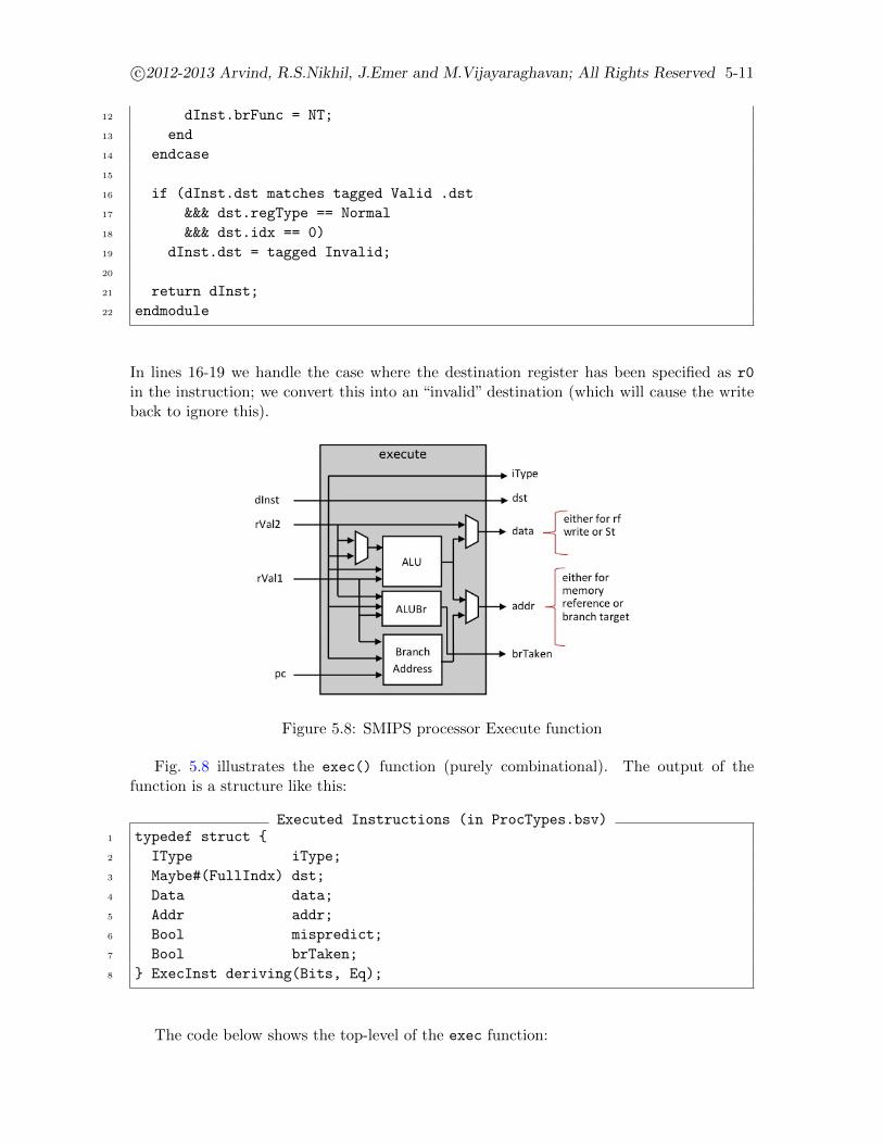
c©2012-2013 Arvind, R.S.Nikhil, J.Emer and M.Vijayaraghavan; All Rights Reserved 5-11
12 dInst.brFunc = NT;
13 end
14 endcase
15
16 if (dInst.dst matches tagged Valid .dst
17 &&& dst.regType == Normal
18 &&& dst.idx == 0)
19 dInst.dst = tagged Invalid;
20
21 return dInst;
22 endmodule
In lines 16-19 we handle the case where the destination register has been specified as r0
in the instruction; we convert this into an “invalid” destination (which will cause the writeback to ignore this).
Figure 5.8: SMIPS processor Execute function
Fig. 5.8 illustrates the exec() function (purely combinational). The output of thefunction is a structure like this:
Executed Instructions (in ProcTypes.bsv)1 typedef struct {
2 IType iType;
3 Maybe#(FullIndx) dst;
4 Data data;
5 Addr addr;
6 Bool mispredict;
7 Bool brTaken;
8 } ExecInst deriving(Bits, Eq);
The code below shows the top-level of the exec function:
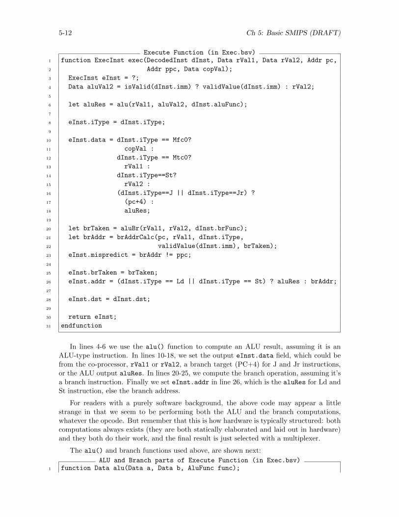
5-12 Ch 5: Basic SMIPS (DRAFT)
Execute Function (in Exec.bsv)1 function ExecInst exec(DecodedInst dInst, Data rVal1, Data rVal2, Addr pc,
2 Addr ppc, Data copVal);
3 ExecInst eInst = ?;
4 Data aluVal2 = isValid(dInst.imm) ? validValue(dInst.imm) : rVal2;
5
6 let aluRes = alu(rVal1, aluVal2, dInst.aluFunc);
7
8 eInst.iType = dInst.iType;
9
10 eInst.data = dInst.iType == Mfc0?
11 copVal :
12 dInst.iType == Mtc0?
13 rVal1 :
14 dInst.iType==St?
15 rVal2 :
16 (dInst.iType==J || dInst.iType==Jr) ?
17 (pc+4) :
18 aluRes;
19
20 let brTaken = aluBr(rVal1, rVal2, dInst.brFunc);
21 let brAddr = brAddrCalc(pc, rVal1, dInst.iType,
22 validValue(dInst.imm), brTaken);
23 eInst.mispredict = brAddr != ppc;
24
25 eInst.brTaken = brTaken;
26 eInst.addr = (dInst.iType == Ld || dInst.iType == St) ? aluRes : brAddr;
27
28 eInst.dst = dInst.dst;
29
30 return eInst;
31 endfunction
In lines 4-6 we use the alu() function to compute an ALU result, assuming it is anALU-type instruction. In lines 10-18, we set the output eInst.data field, which could befrom the co-processor, rVal1 or rVal2, a branch target (PC+4) for J and Jr instructions,or the ALU output aluRes. In lines 20-25, we compute the branch operation, assuming it’sa branch instruction. Finally we set eInst.addr in line 26, which is the aluRes for Ld andSt instruction, else the branch address.
For readers with a purely software background, the above code may appear a littlestrange in that we seem to be performing both the ALU and the branch computations,whatever the opcode. But remember that this is how hardware is typically structured: bothcomputations always exists (they are both statically elaborated and laid out in hardware)and they both do their work, and the final result is just selected with a multiplexer.
The alu() and branch functions used above, are shown next:
ALU and Branch parts of Execute Function (in Exec.bsv)1 function Data alu(Data a, Data b, AluFunc func);
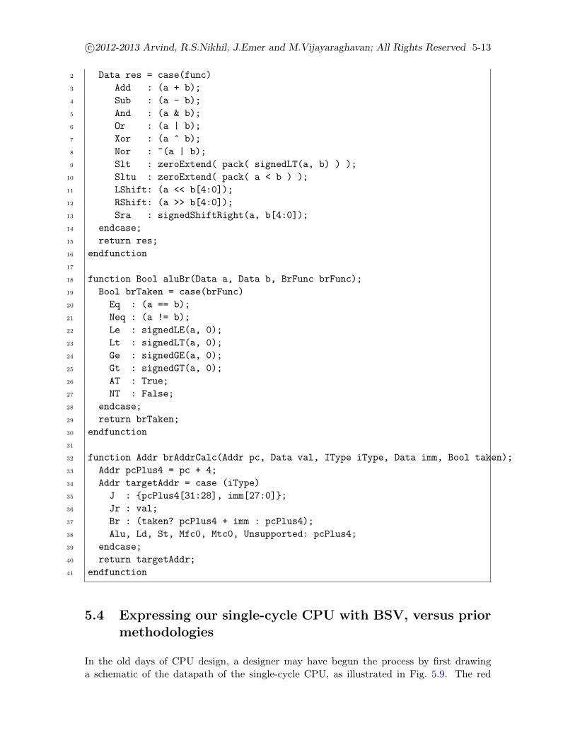
c©2012-2013 Arvind, R.S.Nikhil, J.Emer and M.Vijayaraghavan; All Rights Reserved 5-13
2 Data res = case(func)
3 Add : (a + b);
4 Sub : (a - b);
5 And : (a & b);
6 Or : (a | b);
7 Xor : (a ^ b);
8 Nor : ~(a | b);
9 Slt : zeroExtend( pack( signedLT(a, b) ) );
10 Sltu : zeroExtend( pack( a < b ) );
11 LShift: (a << b[4:0]);
12 RShift: (a >> b[4:0]);
13 Sra : signedShiftRight(a, b[4:0]);
14 endcase;
15 return res;
16 endfunction
17
18 function Bool aluBr(Data a, Data b, BrFunc brFunc);
19 Bool brTaken = case(brFunc)
20 Eq : (a == b);
21 Neq : (a != b);
22 Le : signedLE(a, 0);
23 Lt : signedLT(a, 0);
24 Ge : signedGE(a, 0);
25 Gt : signedGT(a, 0);
26 AT : True;
27 NT : False;
28 endcase;
29 return brTaken;
30 endfunction
31
32 function Addr brAddrCalc(Addr pc, Data val, IType iType, Data imm, Bool taken);
33 Addr pcPlus4 = pc + 4;
34 Addr targetAddr = case (iType)
35 J : {pcPlus4[31:28], imm[27:0]};
36 Jr : val;
37 Br : (taken? pcPlus4 + imm : pcPlus4);
38 Alu, Ld, St, Mfc0, Mtc0, Unsupported: pcPlus4;
39 endcase;
40 return targetAddr;
41 endfunction
5.4 Expressing our single-cycle CPU with BSV, versus priormethodologies
In the old days of CPU design, a designer may have begun the process by first drawinga schematic of the datapath of the single-cycle CPU, as illustrated in Fig. 5.9. The red
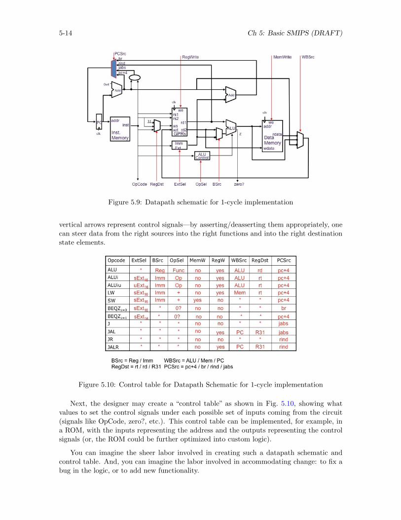
5-14 Ch 5: Basic SMIPS (DRAFT)
Figure 5.9: Datapath schematic for 1-cycle implementation
vertical arrows represent control signals—by asserting/deasserting them appropriately, onecan steer data from the right sources into the right functions and into the right destinationstate elements.
Figure 5.10: Control table for Datapath Schematic for 1-cycle implementation
Next, the designer may create a “control table” as shown in Fig. 5.10, showing whatvalues to set the control signals under each possible set of inputs coming from the circuit(signals like OpCode, zero?, etc.). This control table can be implemented, for example, ina ROM, with the inputs representing the address and the outputs representing the controlsignals (or, the ROM could be further optimized into custom logic).
You can imagine the sheer labor involved in creating such a datapath schematic andcontrol table. And, you can imagine the labor involved in accommodating change: to fix abug in the logic, or to add new functionality.
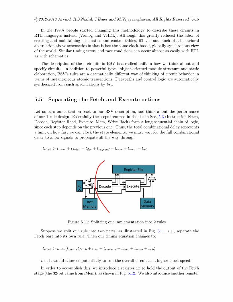
c©2012-2013 Arvind, R.S.Nikhil, J.Emer and M.Vijayaraghavan; All Rights Reserved 5-15
In the 1990s people started changing this methodology to describe these circuits inRTL languages instead (Verilog and VHDL). Although this greatly reduced the labor ofcreating and maintaining schematics and control tables, RTL is not much of a behavioralabstraction above schematics in that it has the same clock-based, globally synchronous viewof the world. Similar timing errors and race conditions can occur almost as easily with RTLas with schematics.
The description of these circuits in BSV is a radical shift in how we think about andspecify circuits. In addition to powerful types, object-oriented module structure and staticelaboration, BSV’s rules are a dramatically different way of thinking of circuit behavior interms of instantaneous atomic transactions. Datapaths and control logic are automaticallysynthesized from such specifications by bsc.
5.5 Separating the Fetch and Execute actions
Let us turn our attention back to our BSV description, and think about the performanceof our 1-rule design. Essentially the steps itemized in the list in Sec. 5.3 (Instruction Fetch,Decode, Register Read, Execute, Mem, Write Back) form a long sequential chain of logic,since each step depends on the previous one. Thus, the total combinational delay representsa limit on how fast we can clock the state elements; we must wait for the full combinationaldelay to allow signals to propagate all the way through:
tclock > tmem + tfetch + tdec + tregread + texec + tmem + twb
Figure 5.11: Splitting our implementation into 2 rules
Suppose we split our rule into two parts, as illustrated in Fig. 5.11, i.e., separate theFetch part into its own rule. Then our timing equation changes to:
tclock > max(tmem, tfetch + tdec + tregread + texec + tmem + twb)
i.e., it would allow us potentially to run the overall circuit at a higher clock speed.
In order to accomplish this, we introduce a register ir to hold the output of the Fetchstage (the 32-bit value from iMem), as shown in Fig. 5.12. We also introduce another register
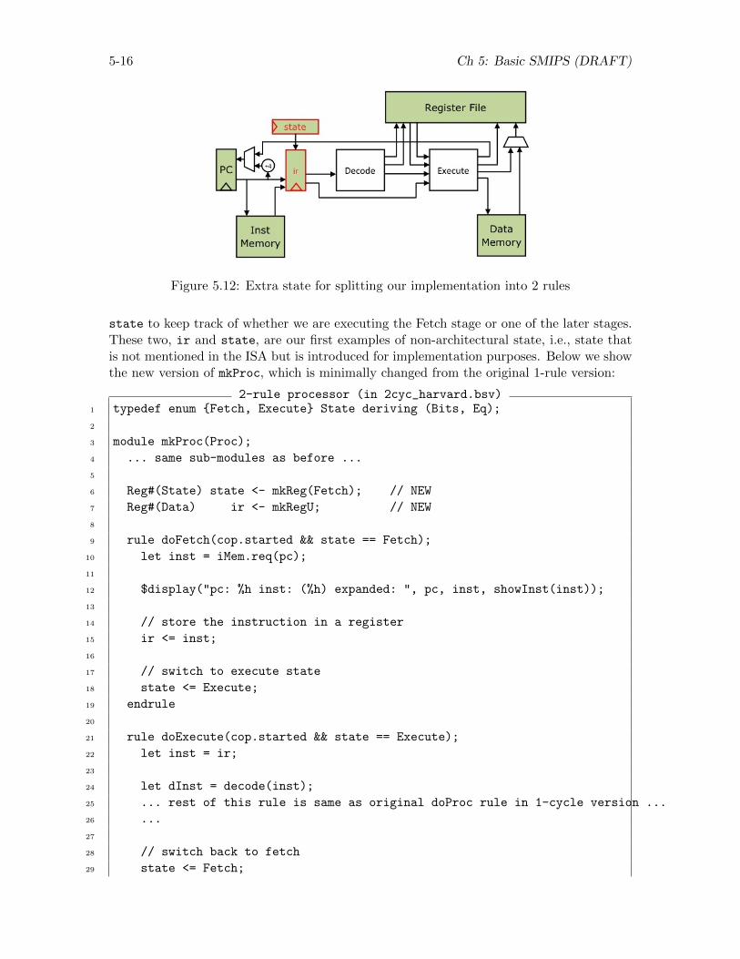
5-16 Ch 5: Basic SMIPS (DRAFT)
Figure 5.12: Extra state for splitting our implementation into 2 rules
state to keep track of whether we are executing the Fetch stage or one of the later stages.These two, ir and state, are our first examples of non-architectural state, i.e., state thatis not mentioned in the ISA but is introduced for implementation purposes. Below we showthe new version of mkProc, which is minimally changed from the original 1-rule version:
2-rule processor (in 2cyc_harvard.bsv)1 typedef enum {Fetch, Execute} State deriving (Bits, Eq);
2
3 module mkProc(Proc);
4 ... same sub-modules as before ...
5
6 Reg#(State) state <- mkReg(Fetch); // NEW
7 Reg#(Data) ir <- mkRegU; // NEW
8
9 rule doFetch(cop.started && state == Fetch);
10 let inst = iMem.req(pc);
11
12 $display("pc: %h inst: (%h) expanded: ", pc, inst, showInst(inst));
13
14 // store the instruction in a register
15 ir <= inst;
16
17 // switch to execute state
18 state <= Execute;
19 endrule
20
21 rule doExecute(cop.started && state == Execute);
22 let inst = ir;
23
24 let dInst = decode(inst);
25 ... rest of this rule is same as original doProc rule in 1-cycle version ...
26 ...
27
28 // switch back to fetch
29 state <= Fetch;
c©2012-2013 Arvind, R.S.Nikhil, J.Emer and M.Vijayaraghavan; All Rights Reserved 5-17
30 endrule
31
32 ...
33 endmodule
Line 1 declares a type for the state of the 2-rule system: it is either in the Fetch rule, orit is in the Execute rule. Inside the module, lines 6-7 instantiate the two new registers stateand |verb|ir|. The original doProc rule is now split into two rules, doFetch and doExecute;we add state==Fetch and state==Execute to the rule conditions. At the end of doFetch,we store the retreived instruction in the ir register and change state to Execute. At thestart of the doExecute rule we retrieve the just-stored instruction from ir, and proceed asbefore. At the end of the rule we set state to Fetch to re-enable the doFetch rule.
Thus, the doFetch and doExecute rules will alternate performing the fetch and executefunctions.
5.5.1 Analysis
Have we really gained anything by splitting into two rules and potentially running themat a faster clock speed? In fact we have not: since the two rules alternate, the total timeto execute an instruction becomes two clock cycles, and unless we were able to more thandouble the clock speed (unlikely!) we will be running no faster than before. And, we’re nowusing more state (and therefore likely more hardware area and power).
However, this exercise has demonstrated one key BSV principle: refinement. In BSV, oneoften refines a design by splitting rules into smaller rules (typically with a goal of increasingclock speed). The strength of rule semantics is that this can often be done independentlyin different parts of a design, i.e., refining a rule typically does not break other parts ofthe design because we typically do not have tight timing assumptions (as is common inRTL languages). This allows us incrementally to refine a design towards meeting particularperformance goals.
This exercise has also set the stage for the real payoff which we shall start exploringin the next chapter, when we start pipelining the two (and more) rules, so that, whilethe Execute rule is doing its thing, the Fetch rule is busy fetching the next instructionconcurrently within the same clock.

5-18 Ch 5: Basic SMIPS (DRAFT)
Chapter 6
SMIPS: Pipelined
We ended the last chapter with a 2-rule version of the basic MIPS processor, illustratedin Fig. 5.12. Other than demonstrating how to refine a BSV program by breaking largerrules into smaller rules, it did not buy us anything either in terms of overall performanceor area. Performance was not improved since the two rules alternate, based on the state
register: the total time per instruction is the same, it just happens in two rules one afterthe other, instead of in one rule. And area likely increased due to the introduction of thenon-architectural state registers state and ir.
In this chapter we will explore how to execute the two rules concurrently (in the sameclock), so that they operate as a pipeline. This should substantially improve the performance(throughput) compared to the original 1-rule version, since the smaller rules should allow usto increase clock speed, and we should be able to complete one instruction on every clock.
6.1 Hazards
When creating a processo pipeline, we typically encounter three kinds of hazards:
• Control Hazards: We do not really know the next instruction to fetch until we haveat least decoded the current instruction. If the decoded instruction is not a branchinstruction, the next instruction is likely to be at PC+4. If it is a branch instruction,we may not know the new PC until the end of the Execute stage. Even if it is not abranch instruction, it may raise an trap/exception later in the pipeline (such as divide-by-zero, or page fault), requiring the next instruction to be from a trap/exceptionhandler.
• Structural Hazard : Two instructions in the pipeline may require the same resourceat the same time. For example, in Princeton architectures, both the Fetch and theExecute stages need to access the same memory.
• Data Hazard : For example, if one instruction writes into register 13, a later instructionthat reads register 13 must wait until the data has been computed and is available.In general, when different stages of the pipeline read and write common state (theregister file being just one example), we must be careful about the order of reads andwrites.
6-1
6-2 Ch 6: SMIPS: Control Hazards (DRAFT)
These are general issues encountered in many kinds of pipelines, not just processors.Simple, pure “feed-forward” pipelines such as the IFFT pipeline of Chapter 4, or an arith-metic multiplier pipeline, typically do not encounter any of these hazards, because thereis no dependence between successive samples flowing through the pipeline. However it isin the very nature of instructions in an ISA that they depend on each other, and so weencounter all these kinds of hazards in their full glory. This leads to significantly morecomplex mechanisms in order to maintain pipeline flow. In fact, dealing with these issuesis the essence of creative computer architecture design.
We will focus on control hazards in this chapter, and address the other types of hazardsin later chapters.
6.1.1 Modern processors are distributed systems
Historically, the Computer Science topic of Distributed Systems grew in the context of LocalArea Networks and Wide Area Networks based on the recognition that, in such systems,communication is not free. In particular,
1. There is no instantly visible or updatable global state. Entities only have local state,and they can only send and receive messages to other entities to query or update remotestate.
2. Messages cannot be delivered instantaneously; there is a discernable latency, and thislatency may not be predictable.
3. Even between the same two entities, messages may get re-ordered, i.e., they may arrivein an order different from the order in which they were sent.
4. Messages may get dropped, spuriously generated, duplicated, or corrupted along theway.
At first glance it may seem startling to refer to a single chip that occupies a few squaremillimeters of silicon (a modern processor or System-on-a-chip) as a “distributed system”,but remember that space and time are relative. Modern processors run at multi-gigahertzspeeds, and communicating across a chip has a discernable delay, and is best addressedby message-passing between relatively independent entities instead of in terms of any glob-ally visible state. Modern chip designers also talk about “GALS” methodology (GloballyAsynchronous, Locally Synchronous), and this is just another manifestation of the sameobservation. Modern system-level communication protocols, such as PCI Express and In-tel’s Quick Path Interconnect (QPI) even deal with the complexities of unreliable messagedelivery (bullet items 3 and 4 above).
In summary, it is fruitful to apply the insights and solutions developed in the field ofDistributed Systems to the design of modern processor architectures. This insight pervadesour approach. In this chapter, the evolution from a globally updated PC to an “epoch”based solution follows this trajectory.
6.2 Two-stage pipelined SMIPS
Fig. 6.1 illustrates a two-stage pipelined version of our SMIPS processor. Let us comparethis with Fig. 5.12. First, we have replaced the “PC+4” function in the Fetch stage with
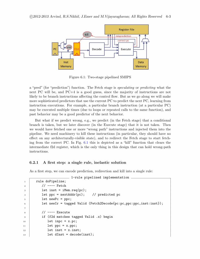
c©2012-2013 Arvind, R.S.Nikhil, J.Emer and M.Vijayaraghavan; All Rights Reserved 6-3
Figure 6.1: Two-stage pipelined SMIPS
a “pred” (for “prediction”) function. The Fetch stage is speculating or predicting what thenext PC will be, and PC+4 is a good guess, since the majority of instructions are notlikely to be branch instructions affecting the control flow. But as we go along we will makemore sophisticated predictors that use the current PC to predict the next PC, learning frominstruction executions. For example, a particular branch instruction (at a particular PC)may be executed multiple times (due to loops or repeated calls to the same function), andpast behavior may be a good predictor of the next behavior.
But what if we predict wrong, e.g., we predict (in the Fetch stage) that a conditionalbranch is taken, but we later discover (in the Execute stage) that it is not taken. Thenwe would have fetched one or more “wrong path” instructions and injected them into thepipeline. We need machinery to kill these instructions (in particular, they should have noeffect on any architecturally-visible state), and to redirect the Fetch stage to start fetch-ing from the correct PC. In Fig. 6.1 this is depicted as a “kill” function that clears theintermediate f2d register, which is the only thing in this design that can hold wrong-pathinstructions.
6.2.1 A first step: a single rule, inelastic solution
As a first step, we can encode prediction, redirection and kill into a single rule:
1-rule pipelined implementation1 rule doPipeline;
2 // ---- Fetch
3 let inst = iMem.req(pc);
4 let ppc = nextAddr(pc); // predicted pc
5 let newPc = ppc;
6 let newIr = tagged Valid (Fetch2Decode{pc:pc,ppc:ppc,inst:inst});
7
8 // ---- Execute
9 if (f2d matches tagged Valid .x) begin
10 let inpc = x.pc;
11 let ppc = x.ppc;
12 let inst = x.inst;
13 let dInst = decode(inst);
6-4 Ch 6: SMIPS: Control Hazards (DRAFT)
14 ... register fetch ...;
15 let eInst = exec(dInst, rVal1, rVal2, inpc, ppc);
16 ...memory operation ...
17 ...register file update ...
18 if (eInst.mispredict) begin
19 newIr = tagged Invalid;
20 newPc = eInst.addr;
21 end
22 end
23 pc <= newPc; f2d <= newIr;
24 endrule
Prediction is encoded in the nextAddr(pc) function, which can be as simple as pc+4.Redirection happens because we initially bind newPC to ppc, but if we encounter a mis-prediction we rebind newPC to the corrected PC (eInst.addr), and we update pc to fi-nal binding of newPc. Killing a wrong-path instruction happens because we initially bindnewIr to the (decoded) predicted instruction, and in the case we discover a misprediction(eInst.mispredict is True) we rebind newIr to tagged Invalid, and this final binding isstored in the f2d register. Pipelining happens because Fetch and Execute both execute ineach rule execution.
This solution works, but is quite complex in lumping all the logic into one big rule. It willbe very difficult to extend this to handle more complex features such as multi-cycle memoryaccesses or functional units, variable latencies due to cache misses and data-dependentfunctional unit latencies, multiple branch predictors and resolvers, etc.
6.2.2 A second step: a two-rule, somewhat elastic solution
A more modular solution would be to evolve towards an elastic pipeline with FIFO coupling,as discussed in Chapter 4. Let us now think of f2d not as a register with a Valid bit, butas a FIFO with enq, first, deq and clear methods. The new code will look like this:
2-rule pipelined implementation1 rule doFetch;
2 let inst = iMem.req(pc);
3 let ppc = nextAddr(pc); // predicted pc
4 pc <= ppc;
5 f2d.enq (tagged Valid (Fetch2Decode{pc:pc,ppc:ppc,inst:inst}));
6 endrule
7
8 rule doExecute;
9 let x = f2d.first;
10 let inpc = x.pc;
11 let ppc = x.ppc;
12 let inst = x.inst;
13 let dInst = decode(inst);
14 ... register fetch ...;
15 let eInst = exec(dInst, rVal1, rVal2, inpc, ppc);
c©2012-2013 Arvind, R.S.Nikhil, J.Emer and M.Vijayaraghavan; All Rights Reserved 6-5
16 ...memory operation ...
17 ...register file update ...
18 if (eInst.mispredict) begin
19 pc <= eInst.addr;
20 f2d.clear;
21 end
22 else
23 f2d.deq;
24 endrule
The doFetch rule now immediately updates pc to the predicted value. In the doExecuterule, when we encounter a misprediction (eInst.mispredic is True), we write the correctvalue into the pc register and simultaneously clear the f2d FIFO.
Can these rules execute concurrently, assuming the FIFO f2d allows concurrent invo-cations of its methods enq, first, deq and clear? The answer is yes, but there are manysubtleties about what we mean by “concurrent”, which are explored in detail in Chapter 7.
The key point to note here is that atomicity of rules guarantees correct operation. RuledoFetch contains three activities, F1: read pc, F2: write pc, and F3: update f2d. RuledoExecute contains two activities, E1: write pc and E2: update f2d. Anyone who hasdone any parallel programming will immediately recognize this as a potentially dangeroussituation. If F1, F2, and F3 can interleave with E1 and E2, bad things can happen: Forexample, the interleaving F1,E1,F2 can leave a mispredicted value in pc. The interleavingF1,F2,E1,E2,F3 can leave a mispredicted instruction in f2d. Such interleavings are ruledout by atomicity of rules— either E1,E2,E3 happen before F1,F2, or vice versa; either way,we get correct operation.
This 2-rule solution is more elastic and decoupled than the previous 1-rule solution,but it still has a number of features which will not scale well to more complex pipelines.First, the Fetch and Execute sections (each of which will themselves evolve into multi-stagepipelines later) both access a common piece of global state, the pc, and we are relying onan instantaneous update to manage redirection on misprediction.
Second, f2d was the only piece of state holding speculative instructions, which couldbe killed with a simple FIFO clear operation. As we evolve to deeper pipelines, there willbe multiple state elements holding speculative instructions, and we may be nested severallevels deep in branch predictions so that when a branch resolves we must kill only some,and not all of the speculative instructions. It will be hard to perform all this activity in asingle, instantaneous, atomic action.
6.2.3 A third step: a two-rule, elastic solution using epochs
We first relax one aspect of our tight coupling, where we instantly kill all speculative instruc-tions as soon as we discover a misprediction. We add an “epoch” register to the processorstate in the Fetch stage, as illustrated in Fig. 6.2. Let’s assume its value is initially 0. TheFetch stage attaches the value in this register to every instruction it sends into f2d. In theExecute stage, we do two new things:
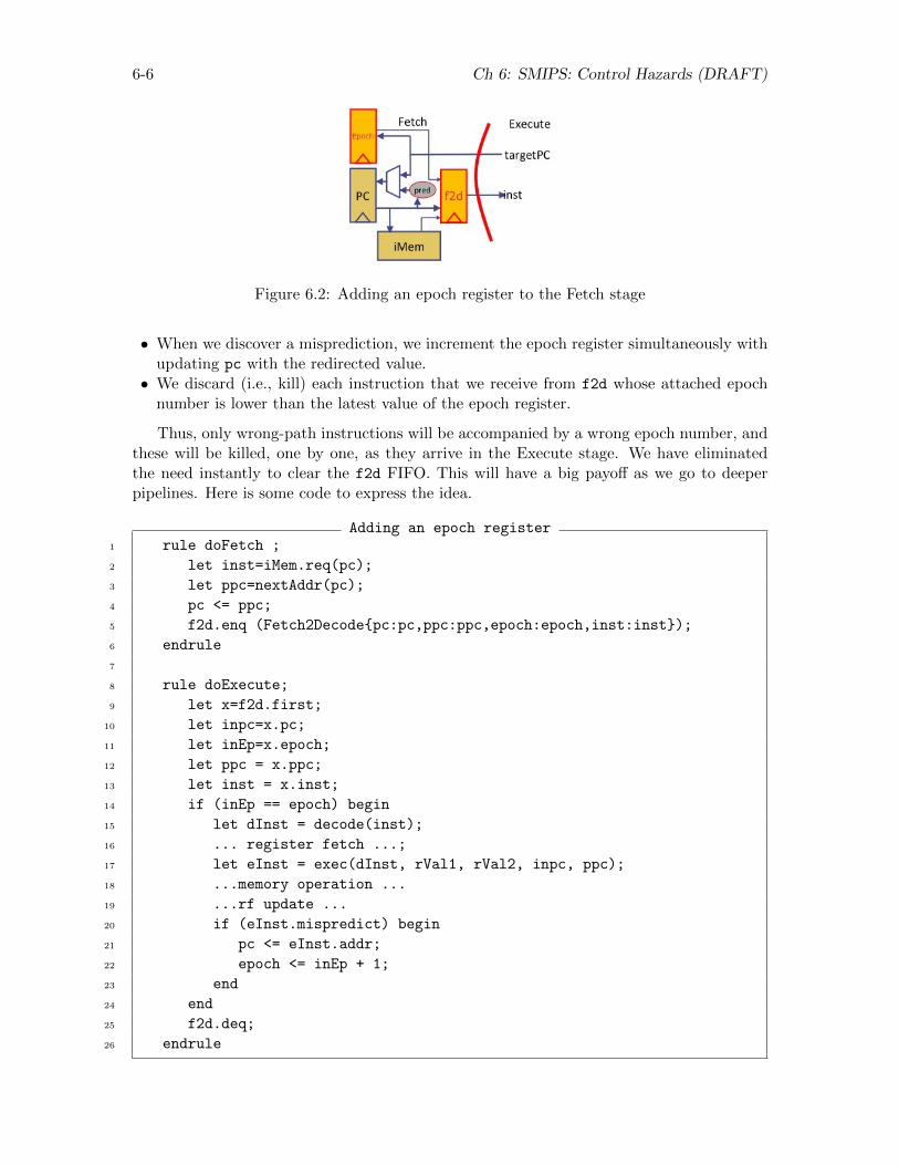
6-6 Ch 6: SMIPS: Control Hazards (DRAFT)
Figure 6.2: Adding an epoch register to the Fetch stage
• When we discover a misprediction, we increment the epoch register simultaneously withupdating pc with the redirected value.
• We discard (i.e., kill) each instruction that we receive from f2d whose attached epochnumber is lower than the latest value of the epoch register.
Thus, only wrong-path instructions will be accompanied by a wrong epoch number, andthese will be killed, one by one, as they arrive in the Execute stage. We have eliminatedthe need instantly to clear the f2d FIFO. This will have a big payoff as we go to deeperpipelines. Here is some code to express the idea.
Adding an epoch register1 rule doFetch ;
2 let inst=iMem.req(pc);
3 let ppc=nextAddr(pc);
4 pc <= ppc;
5 f2d.enq (Fetch2Decode{pc:pc,ppc:ppc,epoch:epoch,inst:inst});
6 endrule
7
8 rule doExecute;
9 let x=f2d.first;
10 let inpc=x.pc;
11 let inEp=x.epoch;
12 let ppc = x.ppc;
13 let inst = x.inst;
14 if (inEp == epoch) begin
15 let dInst = decode(inst);
16 ... register fetch ...;
17 let eInst = exec(dInst, rVal1, rVal2, inpc, ppc);
18 ...memory operation ...
19 ...rf update ...
20 if (eInst.mispredict) begin
21 pc <= eInst.addr;
22 epoch <= inEp + 1;
23 end
24 end
25 f2d.deq;
26 endrule
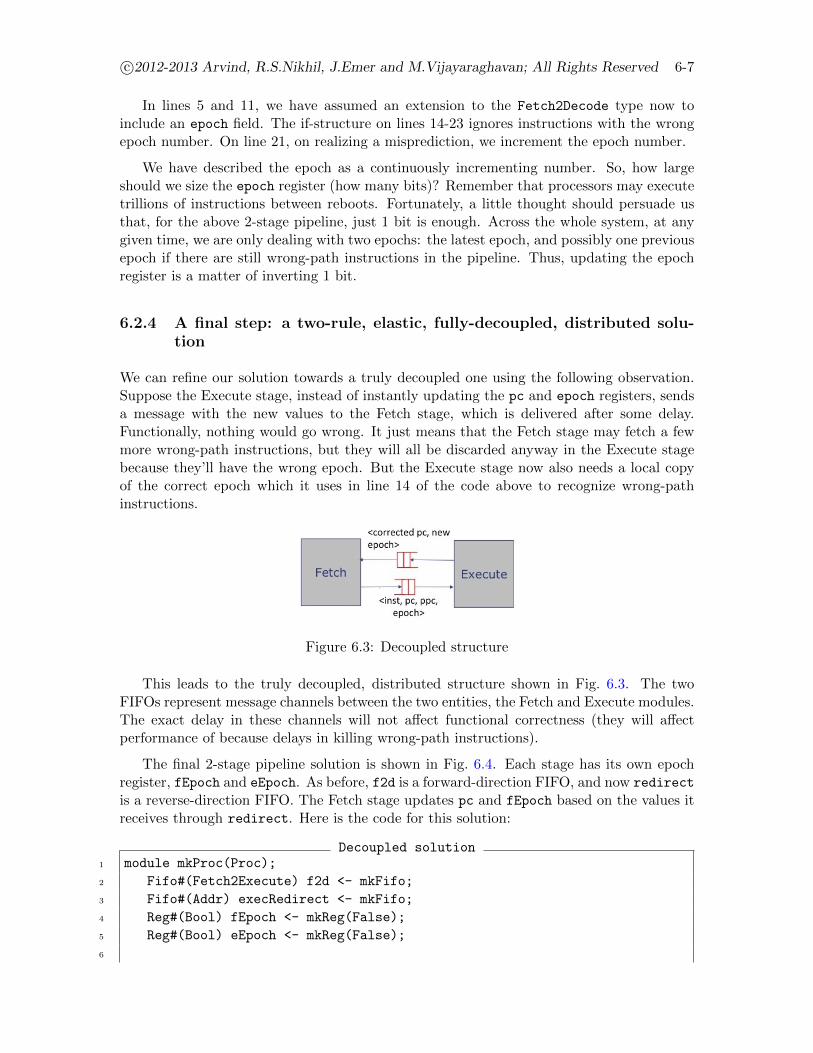
c©2012-2013 Arvind, R.S.Nikhil, J.Emer and M.Vijayaraghavan; All Rights Reserved 6-7
In lines 5 and 11, we have assumed an extension to the Fetch2Decode type now toinclude an epoch field. The if-structure on lines 14-23 ignores instructions with the wrongepoch number. On line 21, on realizing a misprediction, we increment the epoch number.
We have described the epoch as a continuously incrementing number. So, how largeshould we size the epoch register (how many bits)? Remember that processors may executetrillions of instructions between reboots. Fortunately, a little thought should persuade usthat, for the above 2-stage pipeline, just 1 bit is enough. Across the whole system, at anygiven time, we are only dealing with two epochs: the latest epoch, and possibly one previousepoch if there are still wrong-path instructions in the pipeline. Thus, updating the epochregister is a matter of inverting 1 bit.
6.2.4 A final step: a two-rule, elastic, fully-decoupled, distributed solu-tion
We can refine our solution towards a truly decoupled one using the following observation.Suppose the Execute stage, instead of instantly updating the pc and epoch registers, sendsa message with the new values to the Fetch stage, which is delivered after some delay.Functionally, nothing would go wrong. It just means that the Fetch stage may fetch a fewmore wrong-path instructions, but they will all be discarded anyway in the Execute stagebecause they’ll have the wrong epoch. But the Execute stage now also needs a local copyof the correct epoch which it uses in line 14 of the code above to recognize wrong-pathinstructions.
Figure 6.3: Decoupled structure
This leads to the truly decoupled, distributed structure shown in Fig. 6.3. The twoFIFOs represent message channels between the two entities, the Fetch and Execute modules.The exact delay in these channels will not affect functional correctness (they will affectperformance of because delays in killing wrong-path instructions).
The final 2-stage pipeline solution is shown in Fig. 6.4. Each stage has its own epochregister, fEpoch and eEpoch. As before, f2d is a forward-direction FIFO, and now redirect
is a reverse-direction FIFO. The Fetch stage updates pc and fEpoch based on the values itreceives through redirect. Here is the code for this solution:
Decoupled solution1 module mkProc(Proc);
2 Fifo#(Fetch2Execute) f2d <- mkFifo;
3 Fifo#(Addr) execRedirect <- mkFifo;
4 Reg#(Bool) fEpoch <- mkReg(False);
5 Reg#(Bool) eEpoch <- mkReg(False);
6
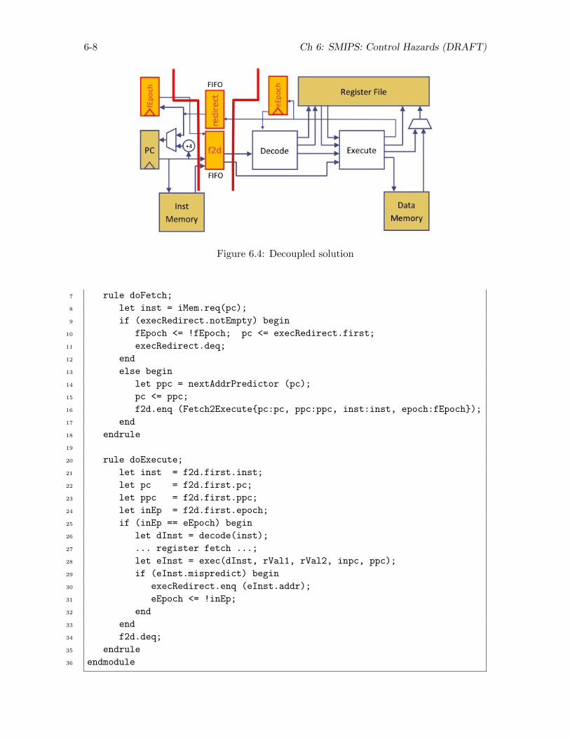
6-8 Ch 6: SMIPS: Control Hazards (DRAFT)
Figure 6.4: Decoupled solution
7 rule doFetch;
8 let inst = iMem.req(pc);
9 if (execRedirect.notEmpty) begin
10 fEpoch <= !fEpoch; pc <= execRedirect.first;
11 execRedirect.deq;
12 end
13 else begin
14 let ppc = nextAddrPredictor (pc);
15 pc <= ppc;
16 f2d.enq (Fetch2Execute{pc:pc, ppc:ppc, inst:inst, epoch:fEpoch});
17 end
18 endrule
19
20 rule doExecute;
21 let inst = f2d.first.inst;
22 let pc = f2d.first.pc;
23 let ppc = f2d.first.ppc;
24 let inEp = f2d.first.epoch;
25 if (inEp == eEpoch) begin
26 let dInst = decode(inst);
27 ... register fetch ...;
28 let eInst = exec(dInst, rVal1, rVal2, inpc, ppc);
29 if (eInst.mispredict) begin
30 execRedirect.enq (eInst.addr);
31 eEpoch <= !inEp;
32 end
33 end
34 f2d.deq;
35 endrule
36 endmodule
c©2012-2013 Arvind, R.S.Nikhil, J.Emer and M.Vijayaraghavan; All Rights Reserved 6-9
Since we need only 1 bit to represent an epoch, and since epoch numbers always togglebetween 0 and 1, we don’t actually have to carry any epoch number on a redirect mes-sage. The very arrival of the message is a signal to toggle it. Thus, the redirect queue(execRedirect) only carries PC values.
In the Fetch rule, if there is any message in the redirect queue, we update pc and fEpoch
(toggle it). Otherwise, we perform the normal instruction fetch and send it into f2d. In theExecute rule, on line 25, if the instruction’s epoch is not equal to the actual current epocheEpoch, we ignore the instruction. If we resolve a misprediction we send eInst.addr backto the Fetch stage via the execRedirect queue, and immediately update the local, actualepoch number eEpoch.
If we revert back for a moment to the abstract idea that the epoch is a continuouslyincrementing number, notice that fEpoch is an approximation of the real epoch, eEpoch.Further, it is always true that fEpoch≤eEpoch, i.e., it always approximates it from below,giving us safe behavior. In later chapters, as we refine to more pipeline stages and havemore sophisticated speculation, each stage will have its own copy of the epoch number, andthis property will continue to hold, i.e., each stage’s local epoch register will approximatefrom below the epoch registers of downstream stages.
6.3 Conclusion
In this chapter we developed a decoupled 2-stage SMIPS pipeline implementation, illus-trating the principle of treating the design as a distributed system of independent entitiescommunicating only with messages. Decoupling simplifies reasoning about correctness, andsimplifies the independent refinement of entities (stages) for higher performance. We havestill been somewhat informal about what we mean by “concurrent” execution of rules (whichis necessary for actually getting pipelined behavior); this will be addressed in the chapteron rule semantics.

6-10 Ch 6: SMIPS: Control Hazards (DRAFT)
Chapter 7
Rule Semantics and EventOrdering
Parallelism within rules, and Concurrent rules within clocks
7.1 Introduction
We now examine rule semantics in more detail, which we have discussed informally so far.In particular, we will examine two key semantic questions:
• What actions can be combined into an individual rule, and what does it mean to executea rule?• What rules can execute within a clock cycle; in what order, and what does it mean?
We will see that in both cases, it comes down to a fairly simple consideration on orderingconstraints on pairs of methods.
We use the words“simultaneous”and“parallel” to refer to the instantaneous execution ofall actions within a rule. We use the word “concurrent” to refer to the execution of multiplerules within a clock. Even though multiple rules may execute in a single clock period, inBSV semantics they will still have a logical sequential order.
We have also used the word “action” informally so far to refer to the actions in a rule.In fact, BSV has a type Action (and a more general type called ActionValue); the bodyof a rule has Action type, and many methods have Action and ActionValue type. Beingformal types in BSV, one can even write expressions and functions of type Action andActionValue.
7.2 Parallelism: semantics of a rule in isolation
A rule can be executed only if its rule condition is true. By this we mean the net, overallcondition of the rule, combining any explicit user-supplied predicate and all the method
7-1
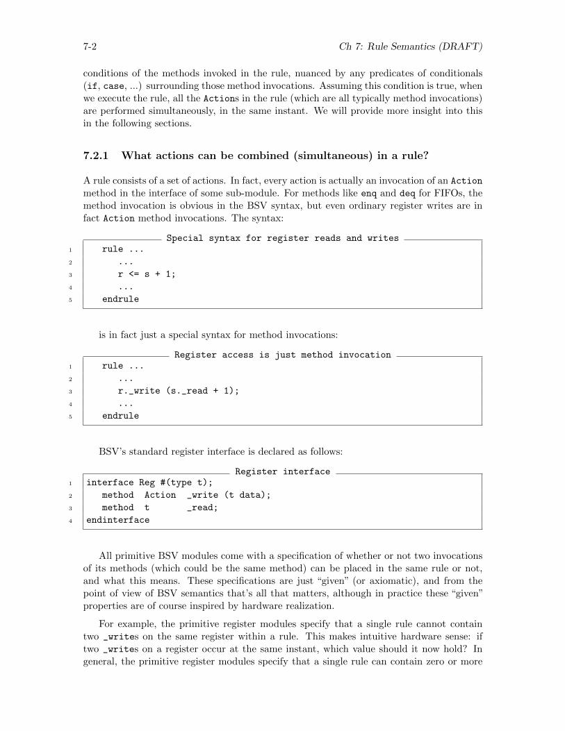
7-2 Ch 7: Rule Semantics (DRAFT)
conditions of the methods invoked in the rule, nuanced by any predicates of conditionals(if, case, ...) surrounding those method invocations. Assuming this condition is true, whenwe execute the rule, all the Actions in the rule (which are all typically method invocations)are performed simultaneously, in the same instant. We will provide more insight into thisin the following sections.
7.2.1 What actions can be combined (simultaneous) in a rule?
A rule consists of a set of actions. In fact, every action is actually an invocation of an Action
method in the interface of some sub-module. For methods like enq and deq for FIFOs, themethod invocation is obvious in the BSV syntax, but even ordinary register writes are infact Action method invocations. The syntax:
Special syntax for register reads and writes1 rule ...
2 ...
3 r <= s + 1;
4 ...
5 endrule
is in fact just a special syntax for method invocations:
Register access is just method invocation1 rule ...
2 ...
3 r._write (s._read + 1);
4 ...
5 endrule
BSV’s standard register interface is declared as follows:
Register interface1 interface Reg #(type t);
2 method Action _write (t data);
3 method t _read;
4 endinterface
All primitive BSV modules come with a specification of whether or not two invocationsof its methods (which could be the same method) can be placed in the same rule or not,and what this means. These specifications are just “given” (or axiomatic), and from thepoint of view of BSV semantics that’s all that matters, although in practice these “given”properties are of course inspired by hardware realization.
For example, the primitive register modules specify that a single rule cannot containtwo _writes on the same register within a rule. This makes intuitive hardware sense: iftwo _writes on a register occur at the same instant, which value should it now hold? Ingeneral, the primitive register modules specify that a single rule can contain zero or more
c©2012-2013 Arvind, R.S.Nikhil, J.Emer and M.Vijayaraghavan; All Rights Reserved 7-3
_reads and/or a single _write on any particular register. It specifies the meaning of each_read as returning the value that was in the register just before the rule execution instant,and the meaning of a _write Action as leaving its argument value in the register just afterthe rule execution instant.
Similarly, FIFO modules will specify that you cannot have two enqs on the same FIFOin the same rule (if they are simultaneous, in what order are they enqueued?).
Although these constraints and meanings are “given”, or axiomatic, for primitive mod-ules, they logically imply similar constraints on user-defined modules (which, ultimately,must be built with primitive modules either directly or indirectly). For example if a modulehas two methods m1 and m2 which both write into a common register, the constraints andmeaning of the underlying _writes carry upward to m1 and m2.
Constraints on methods of primitive or user-defined modules may also arise due to hard-ware resource limitations. For example, a method m3(x), when implemented in hardware,may have a single input bus for x; this bus can only be driven with one value at a time;thus, it would not make sense to have two invocations of m3 within a single rule.
In summary: we can place any actions into a rule for simultaneous execution, providedwe respect such (mostly obvious) constraints. The bsc compiler will flag any violations asa static, compile-time error.
Examples of legal and illegal combinations of actions into rules
Example 1:
Parallel methods in a rule1 rule ra if (z>10);
2 x <= x+1;
3 endrule
This rule is fine: a read and a write on register x is ok, as is a read from register z.
Example 2:
Parallel methods in a rule1 rule rb;
2 x <= x+1;
3 if (p) x <= 7;
4 endrule
This rule is not ok, since it potentially performs two writes on regster x. bsc will acceptit only in the trivial case where it can statically prove that p is false.
7-4 Ch 7: Rule Semantics (DRAFT)
Example 3:
Parallel methods in a rule1 rule rb;
2 if (q)
3 x <= x+1;
4 else
5 x <= 7;
6 endrule
This rule is ok. Even though there are two syntatic occurrences of a write to x, theyare in the context of a conditional which ensures that only one of them will be performed.It is equivalent to a more explicit muxed expression:
Parallel methods in a rule1 rule rb;
2 x <= (q ? x+1 : 7);
3 endrule
Example 4:
Parallel methods in a rule1 rule rc;
2 x <= y+1;
3 y <= x+2;
4 endrule
This rule is ok, since it contains one read and one write for each of x and y. Accordingto the given (axiomatic) semantics of the _read and _write methods, both reads of x and y
read the value just before the rule execution instant, and both writes of x and y will updatethe registers with values visible just after the execution instant. Thus, this rule does a kindof “exchange and increment” of x and y, incrementing by 2 and 1, respectively.
Example 5:
Parallel methods in a rule1 rule rd;
2 let t1 = f (t2);
3 let t2 = g (t1);
4 x <= t1;
5 endrule
This rule will not be ok because it likely represents a combinational cycle (note that theoutput of each function is fed into the input of the other). bsc checks for combinationalcycles and raises a compile time error if found.
c©2012-2013 Arvind, R.S.Nikhil, J.Emer and M.Vijayaraghavan; All Rights Reserved 7-5
Example 6:
Parallel methods in a rule1 rule re;
2 s2 = f (s1);
3 s3 = g (s2);
4 x <= s3;
5 endrule
This rule will be ok if it is ok to call f and g simultaneously. For example, if f andg are ordinary arithmetic functions, there is no problem. Even if f and g are the samearithmetic function, the logic will simply be replicated. However, suppose f and g containcalls to a method on some hardware module (such as reading a single port in a register filebut with different indexes); then that method will have a constraint that it cannot be calledsimultaneously, and the rule will not be ok. This constraint is likely driven by the hardwareconstraint that s1 and s2 are input wires into the module, and can only carry one value inany particular instant.
7.2.2 Execution semantics of a single rule
A rule can be seen as a specification of an acyclic combinational circuit whose inputs andoutputs are connected to the interface methods of sub-modules invoked in the rule. Pleaserefer to Figs. 3.7 and 3.8 to refresh your memory about how interface methods map to inputand output wires of a module. Also recall that for any Action or ActionValue method,there is an input “enable” wire (“EN”); when this wire is asserted the method’s action isperformed inside the module. For example, consider this rule:
Simple example for 1-rule semantics1 rule rf (mod1.f > 3);
2 x <= x+1;
3 if (x != 0) y <= x >> 7;
4 endrule
Figure 7.1: Combinational circuit for a rule
Fig. 7.1 illustrates the combinational circuit, or the “data flow graph” for this rule. Themethod mod1.f can only be invoked when it is enabled (its RDY signal is true). This ishandled by the AND gate on the left. The CAN FIRE signal is a boolean indicating whether
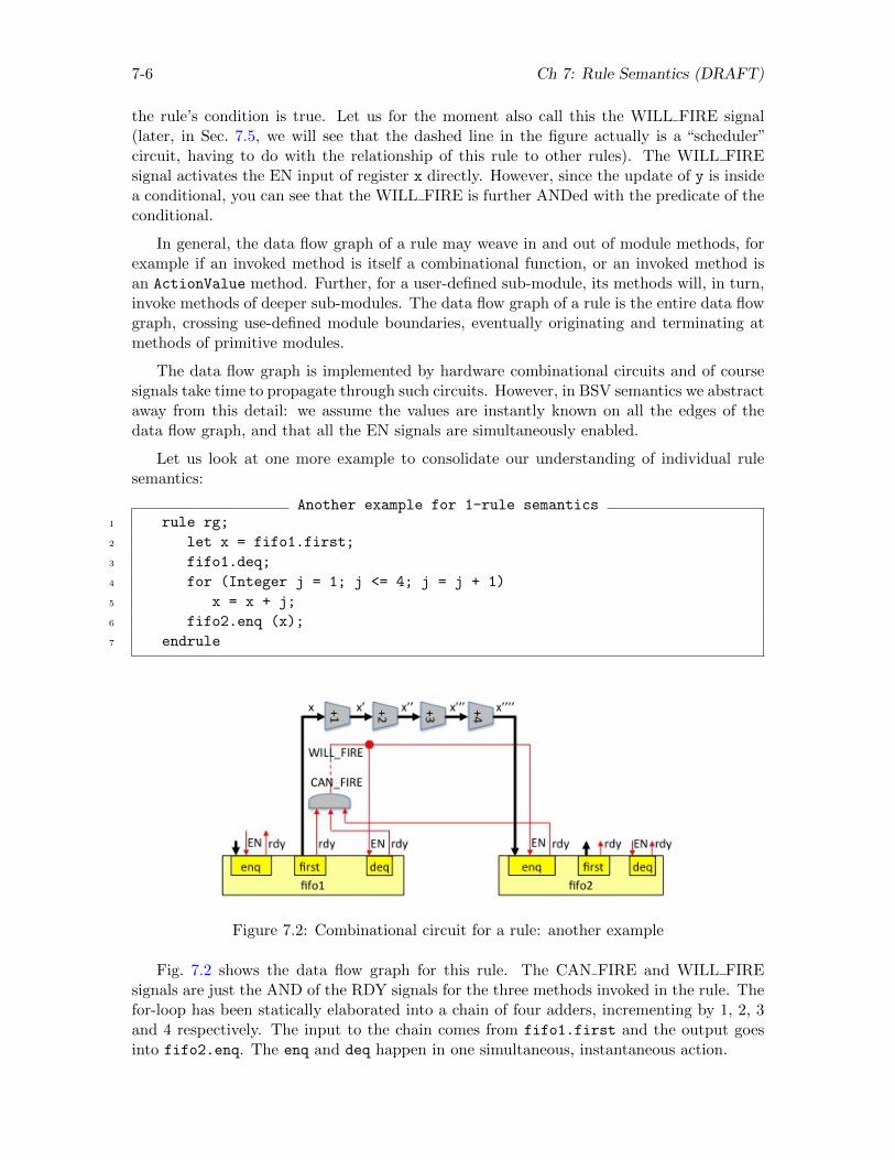
7-6 Ch 7: Rule Semantics (DRAFT)
the rule’s condition is true. Let us for the moment also call this the WILL FIRE signal(later, in Sec. 7.5, we will see that the dashed line in the figure actually is a “scheduler”circuit, having to do with the relationship of this rule to other rules). The WILL FIREsignal activates the EN input of register x directly. However, since the update of y is insidea conditional, you can see that the WILL FIRE is further ANDed with the predicate of theconditional.
In general, the data flow graph of a rule may weave in and out of module methods, forexample if an invoked method is itself a combinational function, or an invoked method isan ActionValue method. Further, for a user-defined sub-module, its methods will, in turn,invoke methods of deeper sub-modules. The data flow graph of a rule is the entire data flowgraph, crossing use-defined module boundaries, eventually originating and terminating atmethods of primitive modules.
The data flow graph is implemented by hardware combinational circuits and of coursesignals take time to propagate through such circuits. However, in BSV semantics we abstractaway from this detail: we assume the values are instantly known on all the edges of thedata flow graph, and that all the EN signals are simultaneously enabled.
Let us look at one more example to consolidate our understanding of individual rulesemantics:
Another example for 1-rule semantics1 rule rg;
2 let x = fifo1.first;
3 fifo1.deq;
4 for (Integer j = 1; j <= 4; j = j + 1)
5 x = x + j;
6 fifo2.enq (x);
7 endrule
Figure 7.2: Combinational circuit for a rule: another example
Fig. 7.2 shows the data flow graph for this rule. The CAN FIRE and WILL FIREsignals are just the AND of the RDY signals for the three methods invoked in the rule. Thefor-loop has been statically elaborated into a chain of four adders, incrementing by 1, 2, 3and 4 respectively. The input to the chain comes from fifo1.first and the output goesinto fifo2.enq. The enq and deq happen in one simultaneous, instantaneous action.
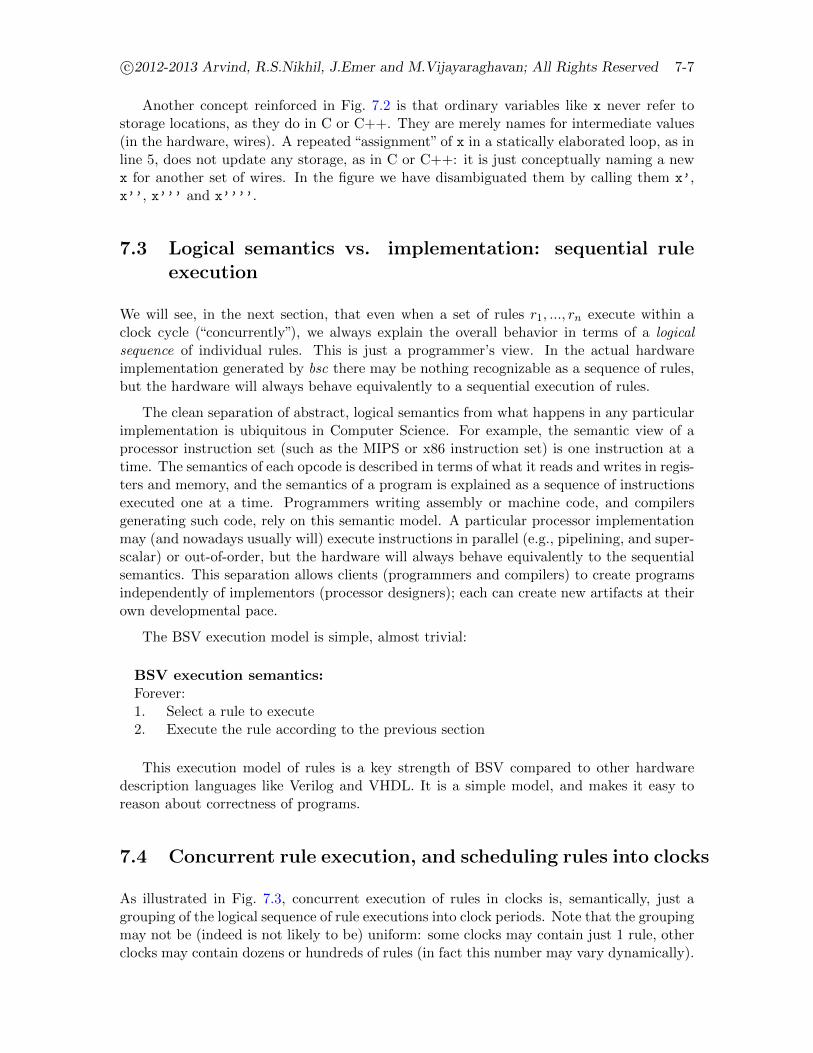
c©2012-2013 Arvind, R.S.Nikhil, J.Emer and M.Vijayaraghavan; All Rights Reserved 7-7
Another concept reinforced in Fig. 7.2 is that ordinary variables like x never refer tostorage locations, as they do in C or C++. They are merely names for intermediate values(in the hardware, wires). A repeated “assignment” of x in a statically elaborated loop, as inline 5, does not update any storage, as in C or C++: it is just conceptually naming a newx for another set of wires. In the figure we have disambiguated them by calling them x’,x’’, x’’’ and x’’’’.
7.3 Logical semantics vs. implementation: sequential ruleexecution
We will see, in the next section, that even when a set of rules r1, ..., rn execute within aclock cycle (“concurrently”), we always explain the overall behavior in terms of a logicalsequence of individual rules. This is just a programmer’s view. In the actual hardwareimplementation generated by bsc there may be nothing recognizable as a sequence of rules,but the hardware will always behave equivalently to a sequential execution of rules.
The clean separation of abstract, logical semantics from what happens in any particularimplementation is ubiquitous in Computer Science. For example, the semantic view of aprocessor instruction set (such as the MIPS or x86 instruction set) is one instruction at atime. The semantics of each opcode is described in terms of what it reads and writes in regis-ters and memory, and the semantics of a program is explained as a sequence of instructionsexecuted one at a time. Programmers writing assembly or machine code, and compilersgenerating such code, rely on this semantic model. A particular processor implementationmay (and nowadays usually will) execute instructions in parallel (e.g., pipelining, and super-scalar) or out-of-order, but the hardware will always behave equivalently to the sequentialsemantics. This separation allows clients (programmers and compilers) to create programsindependently of implementors (processor designers); each can create new artifacts at theirown developmental pace.
The BSV execution model is simple, almost trivial:
BSV execution semantics:Forever:1. Select a rule to execute2. Execute the rule according to the previous section
This execution model of rules is a key strength of BSV compared to other hardwaredescription languages like Verilog and VHDL. It is a simple model, and makes it easy toreason about correctness of programs.
7.4 Concurrent rule execution, and scheduling rules into clocks
As illustrated in Fig. 7.3, concurrent execution of rules in clocks is, semantically, just agrouping of the logical sequence of rule executions into clock periods. Note that the groupingmay not be (indeed is not likely to be) uniform: some clocks may contain just 1 rule, otherclocks may contain dozens or hundreds of rules (in fact this number may vary dynamically).
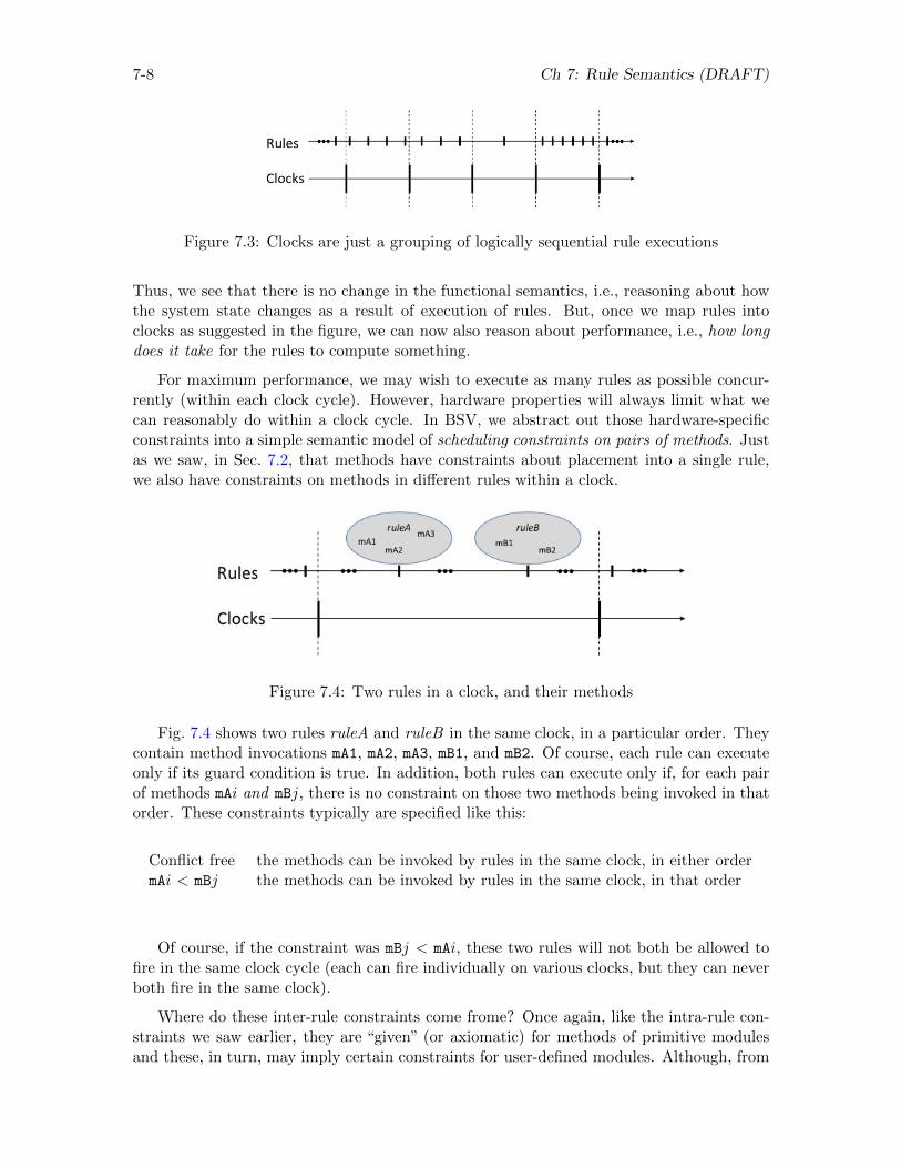
7-8 Ch 7: Rule Semantics (DRAFT)
Figure 7.3: Clocks are just a grouping of logically sequential rule executions
Thus, we see that there is no change in the functional semantics, i.e., reasoning about howthe system state changes as a result of execution of rules. But, once we map rules intoclocks as suggested in the figure, we can now also reason about performance, i.e., how longdoes it take for the rules to compute something.
For maximum performance, we may wish to execute as many rules as possible concur-rently (within each clock cycle). However, hardware properties will always limit what wecan reasonably do within a clock cycle. In BSV, we abstract out those hardware-specificconstraints into a simple semantic model of scheduling constraints on pairs of methods. Justas we saw, in Sec. 7.2, that methods have constraints about placement into a single rule,we also have constraints on methods in different rules within a clock.
Figure 7.4: Two rules in a clock, and their methods
Fig. 7.4 shows two rules ruleA and ruleB in the same clock, in a particular order. Theycontain method invocations mA1, mA2, mA3, mB1, and mB2. Of course, each rule can executeonly if its guard condition is true. In addition, both rules can execute only if, for each pairof methods mAi and mBj, there is no constraint on those two methods being invoked in thatorder. These constraints typically are specified like this:
Conflict free the methods can be invoked by rules in the same clock, in either ordermAi < mBj the methods can be invoked by rules in the same clock, in that order
Of course, if the constraint was mBj < mAi, these two rules will not both be allowed tofire in the same clock cycle (each can fire individually on various clocks, but they can neverboth fire in the same clock).
Where do these inter-rule constraints come frome? Once again, like the intra-rule con-straints we saw earlier, they are “given” (or axiomatic) for methods of primitive modulesand these, in turn, may imply certain constraints for user-defined modules. Although, from

c©2012-2013 Arvind, R.S.Nikhil, J.Emer and M.Vijayaraghavan; All Rights Reserved 7-9
a semantic point of view, we just take the constaints on primitive modules as “given”, theyare of course, in practice, inspired by hardware implementation constraints.
Consider again the register interface. We have already seen the constraints for combining_read and _write methods within a rule. For concurrent execution, we have the constraint:
_read < _write
We can easily see the hardware intuitions behind this. Within a clock, the value weread from a register is the one from the previous clock edge, and any value we write willonly be visible at the next clock edge. The above constraint allows BSV register _readsand _writes to map naturally onto ordinary hardware register reads and writes. If we hadallowed a rule with a _write to precede another rule with a _read within the same clock,then value written in the first rule would have to be read in the second rule, all within aclock, and this does not map naturally and directly to ordinary hardware registers.
We also use the word “conflict” to describe the situation where the method constraintsimply contradictory rule orderings, i.e., some method constraints require ruleA<ruleB andother method constraints require ruleB<ruleA. Whenever there is a conflict in a set of rules,whether given by primitives or induced like this, those rules cannot execute concurrently.
7.4.1 Schedules, and compilation of schedules
A schedule for a clock cycle is any linear list of rules to be attempted in that clock cycle.It can contain a subset or superset of the rules in a design, including duplicates. Executinga schedule is simple:
Forever (for each clock):1. For each rule in the schedule (in order):
If it is enabledand it has no intra-rule conflictsand it has no inter-rule conflicts with rules already executed in this clock
2. Perform the actions of the rule body
Different schedules can result in different performance. If two rules Ri and Rj are placedin a schedule such that a method ordering constraint is violated, then they can never firein the same clock. Reversing their order in the schedule may allow them to fire in the sameclock. The logical semantics leaves it open to the implementation to choose good schedules.
The bsc compiler performs extensive static analysis of the intra-rule and inter-rule con-straints of a BSV program to create a good schedule, one that maximizes the number ofrules that can execute within each clock. The user can place “attributes” in the source codeto fix certain choices in schedule. Compilation outputs allow the user to view the schedulechosen, both graphically and textually. bsc generates hardware that implements the ruleswith this schedule.
7.4.2 Examples
Let us now firm up this simple idea by looking at a series of examples.

7-10 Ch 7: Rule Semantics (DRAFT)
Example 1
Conflict free example1 rule ra if (z>10);
2 x <= x+1;
3 endrule
4
5 rule rb if (z>20);
6 y <= y+2;
7 endrule
The methods involved are: z._read, x._read, x._write, y._read, and y._write.There are no constraints between x’s methods and y’s methods and z’s methods. There areno constraints between z._read in different rules. Thus, there are no constraints betweenthe rules, and bsc will compile hardware that permits these rules to fire concurrently (ofcourse, only whenever both their rule conditions are true).
Example 2
Conflict example1 rule ra if (z>10);
2 x <= y+1;
3 endrule
4
5 rule rb if (z>20);
6 y <= x+2;
7 endrule
Here, y._read < y._write requires ra to precede rb. But, x._read < x._write re-quires rb to precede ra. This is a conflict, and bsc will ensure that these rules do not fireconcurrently.
Example 3
Conflict-free example1 rule ra if (z>10);
2 x <= y+1;
3 endrule
4
5 rule rb if (z>20);
6 y <= y+2;
7 endrule
Here, y._read < y._write requires ra to precede rb, and that is the only inter-ruleconstraint. bsc will allow these rules to fire concurrently, in the logical order: ra before rb.
c©2012-2013 Arvind, R.S.Nikhil, J.Emer and M.Vijayaraghavan; All Rights Reserved 7-11
Example 4
Conflict example1 rule ra;
2 x <= y+1;
3 u <= u+2;
4 endrule
5
6 rule rb;
7 y <= y+2;
8 v <= u+1;
9 endrule
Here, y._read < y._write requires ra to precede rb. u._read < u._write requiresrb to precede ra. Once again, we have a conflict, and bsc will not allow these rules to fireconcurrently.
Example 5
Conflict-free example1 rule ra (z>10);
2 x <= x+1;
3 endrule
4
5 rule rb if (z>20);
6 x <= 23;
7 endrule
Here, x._read < x._write requires ra to precede rb. The primitive register modulesactually place no inter-rule scheduling constraint between x._write and x._write because:
• between rules there is always a clear logical sequential order;• semantically, the final value in the register is what was written by the last rule in this
order, and• since the order is known statically to bsc, it is trivial to generate hardware to only
perform the write from the last rule.
Thus, there is no conflict in this example, and bsc will allow the rules to execute con-currently with the logical ordering of ra before rb. Note that since the rules have differentfiring conditions, it is possible for rule ra to fire alone, incrementing x; it is only when theyfire together that the increment is discarded and x is set to 23.
This example is sometimes surprising to hardware designers because it might appear asif we were doing two writes to the same register in the same clock. But this is confusinglogical semantics with implementation. Here, the logical semantics is indeed doing twowrites to the register; the implementation does just one. This happens all the time, notjust in BSV! For example, if you wrote a C program with the statements:
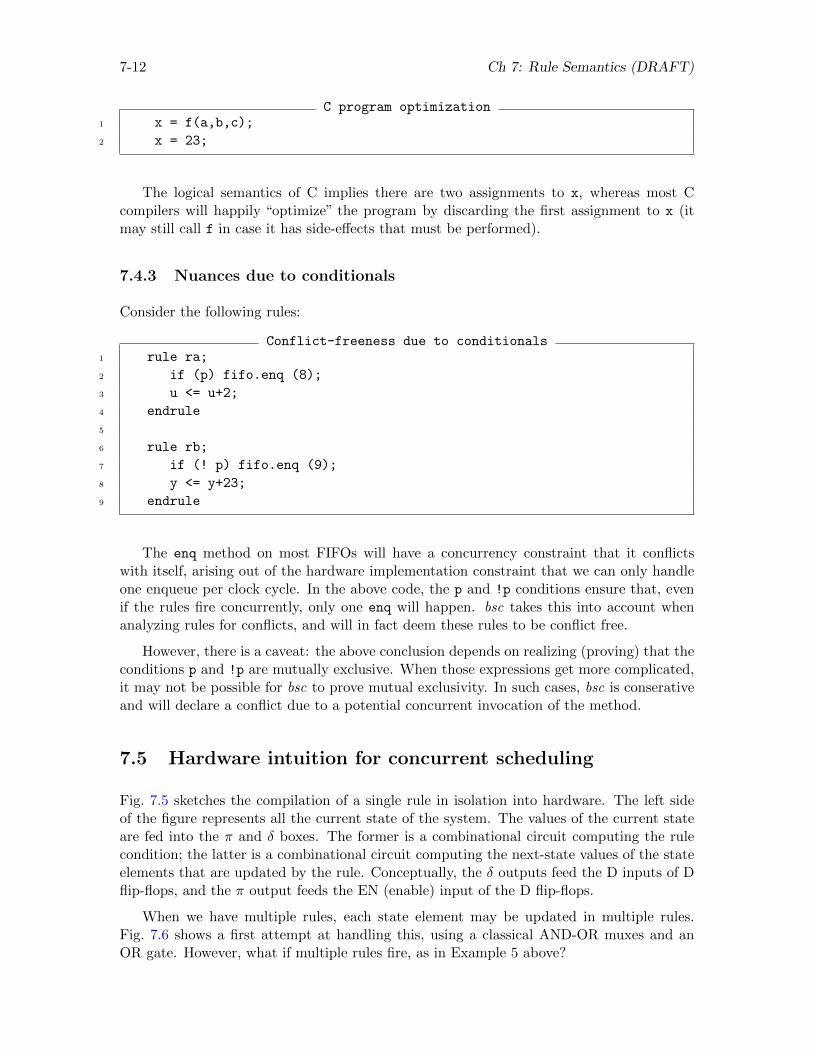
7-12 Ch 7: Rule Semantics (DRAFT)
C program optimization1 x = f(a,b,c);
2 x = 23;
The logical semantics of C implies there are two assignments to x, whereas most Ccompilers will happily “optimize” the program by discarding the first assignment to x (itmay still call f in case it has side-effects that must be performed).
7.4.3 Nuances due to conditionals
Consider the following rules:
Conflict-freeness due to conditionals1 rule ra;
2 if (p) fifo.enq (8);
3 u <= u+2;
4 endrule
5
6 rule rb;
7 if (! p) fifo.enq (9);
8 y <= y+23;
9 endrule
The enq method on most FIFOs will have a concurrency constraint that it conflictswith itself, arising out of the hardware implementation constraint that we can only handleone enqueue per clock cycle. In the above code, the p and !p conditions ensure that, evenif the rules fire concurrently, only one enq will happen. bsc takes this into account whenanalyzing rules for conflicts, and will in fact deem these rules to be conflict free.
However, there is a caveat: the above conclusion depends on realizing (proving) that theconditions p and !p are mutually exclusive. When those expressions get more complicated,it may not be possible for bsc to prove mutual exclusivity. In such cases, bsc is conserativeand will declare a conflict due to a potential concurrent invocation of the method.
7.5 Hardware intuition for concurrent scheduling
Fig. 7.5 sketches the compilation of a single rule in isolation into hardware. The left sideof the figure represents all the current state of the system. The values of the current stateare fed into the π and δ boxes. The former is a combinational circuit computing the rulecondition; the latter is a combinational circuit computing the next-state values of the stateelements that are updated by the rule. Conceptually, the δ outputs feed the D inputs of Dflip-flops, and the π output feeds the EN (enable) input of the D flip-flops.
When we have multiple rules, each state element may be updated in multiple rules.Fig. 7.6 shows a first attempt at handling this, using a classical AND-OR muxes and anOR gate. However, what if multiple rules fire, as in Example 5 above?
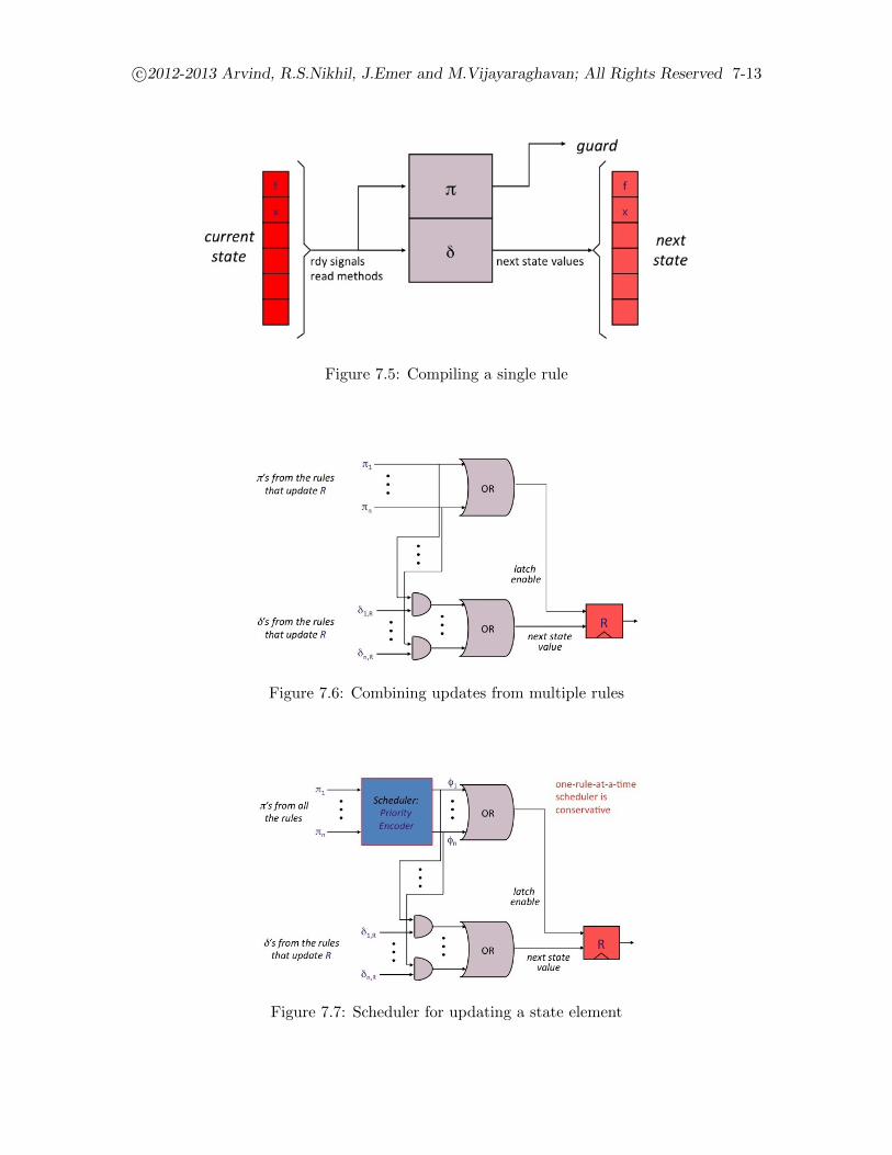
c©2012-2013 Arvind, R.S.Nikhil, J.Emer and M.Vijayaraghavan; All Rights Reserved 7-13
Figure 7.5: Compiling a single rule
Figure 7.6: Combining updates from multiple rules
Figure 7.7: Scheduler for updating a state element
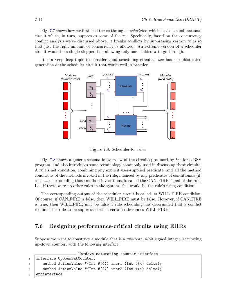
7-14 Ch 7: Rule Semantics (DRAFT)
Fig. 7.7 shows how we first feed the πs through a scheduler, which is also a combinationalcircuit which, in turn, suppresses some of the πs. Specifically, based on the concurrencyconflict analysis we’ve discussed above, it breaks conflicts by suppressing certain rules sothat just the right amount of concurrency is allowed. An extreme version of a schedulercircuit would be a single-stepper, i.e., allowing only one enabled π to go through.
It is a very deep topic to consider good scheduling circuits. bsc has a sophisticatedgeneration of the scheduler circuit that works well in practice.
Figure 7.8: Scheduler for rules
Fig. 7.8 shows a generic schematic overview of the circuits produced by bsc for a BSVprogram, and also introduces some terminology commonly used in discussing these circuits.A rule’s net condition, combining any explicit user-supplied predicate, and all the methodconditions of the methods invoked in the rule, nuanced by any predicates of conditionals (if,case, ...) surrounding those method invocations, is called the CAN FIRE signal of the rule.I.e., if there were no other rules in the system, this would be the rule’s firing condition.
The corresponding output of the scheduler circuit is called its WILL FIRE condition.Of course, if CAN FIRE is false, then WILL FIRE must be false. However, if CAN FIREis true, then WILL FIRE may be false if rule scheduling has determined that a conflictrequires this rule to be suppressed when certain other rules WILL FIRE.
7.6 Designing performance-critical ciruits using EHRs
Suppose we want to construct a module that is a two-port, 4-bit signed integer, saturatingup-down counter, with the following interface:
Up-down saturating counter interface1 interface UpDownSatCounter;
2 method ActionValue #(Int #(4)) incr1 (Int #(4) delta);
3 method ActionValue #(Int #(4)) incr2 (Int #(4) delta);
4 endinterface
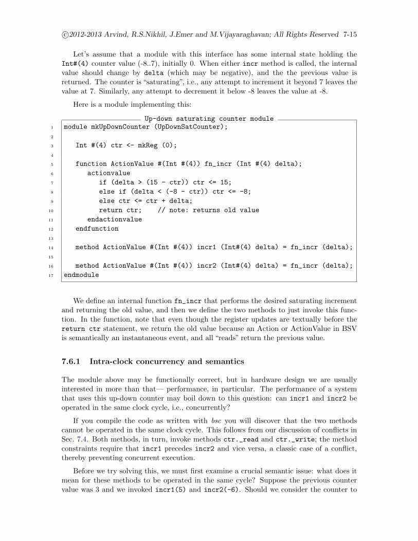
c©2012-2013 Arvind, R.S.Nikhil, J.Emer and M.Vijayaraghavan; All Rights Reserved 7-15
Let’s assume that a module with this interface has some internal state holding theInt#(4) counter value (-8..7), initially 0. When either incr method is called, the internalvalue should change by delta (which may be negative), and the the previous value isreturned. The counter is “saturating”, i.e., any attempt to increment it beyond 7 leaves thevalue at 7. Similarly, any attempt to decrement it below -8 leaves the value at -8.
Here is a module implementing this:
Up-down saturating counter module1 module mkUpDownCounter (UpDownSatCounter);
2
3 Int #(4) ctr <- mkReg (0);
4
5 function ActionValue #(Int #(4)) fn_incr (Int #(4) delta);
6 actionvalue
7 if (delta > (15 - ctr)) ctr <= 15;
8 else if (delta < (-8 - ctr)) ctr <= -8;
9 else ctr <= ctr + delta;
10 return ctr; // note: returns old value
11 endactionvalue
12 endfunction
13
14 method ActionValue #(Int #(4)) incr1 (Int#(4) delta) = fn_incr (delta);
15
16 method ActionValue #(Int #(4)) incr2 (Int#(4) delta) = fn_incr (delta);
17 endmodule
We define an internal function fn_incr that performs the desired saturating incrementand returning the old value, and then we define the two methods to just invoke this func-tion. In the function, note that even though the register updates are textually before thereturn ctr statement, we return the old value because an Action or ActionValue in BSVis semantically an instantaneous event, and all “reads” return the previous value.
7.6.1 Intra-clock concurrency and semantics
The module above may be functionally correct, but in hardware design we are usuallyinterested in more than that— performance, in particular. The performance of a systemthat uses this up-down counter may boil down to this question: can incr1 and incr2 beoperated in the same clock cycle, i.e., concurrently?
If you compile the code as written with bsc you will discover that the two methodscannot be operated in the same clock cycle. This follows from our discussion of conflicts inSec. 7.4. Both methods, in turn, invoke methods ctr._read and ctr._write; the methodconstraints require that incr1 precedes incr2 and vice versa, a classic case of a conflict,thereby preventing concurrent execution.
Before we try solving this, we must first examine a crucial semantic issue: what does itmean for these methods to be operated in the same cycle? Suppose the previous countervalue was 3 and we invoked incr1(5) and incr2(-6). Should we consider the counter to
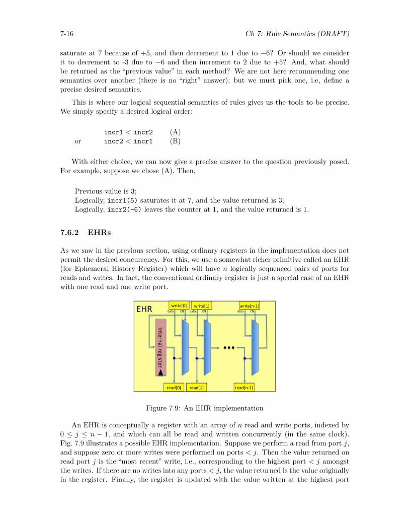
7-16 Ch 7: Rule Semantics (DRAFT)
saturate at 7 because of +5, and then decrement to 1 due to −6? Or should we considerit to decrement to -3 due to −6 and then increment to 2 due to +5? And, what shouldbe returned as the “previous value” in each method? We are not here recommending onesemantics over another (there is no “right” answer); but we must pick one, i.e, define aprecise desired semantics.
This is where our logical sequential semantics of rules gives us the tools to be precise.We simply specify a desired logical order:
incr1 < incr2 (A)or incr2 < incr1 (B)
With either choice, we can now give a precise answer to the question previously posed.For example, suppose we chose (A). Then,
Previous value is 3;Logically, incr1(5) saturates it at 7, and the value returned is 3;Logically, incr2(-6) leaves the counter at 1, and the value returned is 1.
7.6.2 EHRs
As we saw in the previous section, using ordinary registers in the implementation does notpermit the desired concurrency. For this, we use a somewhat richer primitive called an EHR(for Ephemeral History Register) which will have n logically sequenced pairs of ports forreads and writes. In fact, the conventional ordinary register is just a special case of an EHRwith one read and one write port.
Figure 7.9: An EHR implementation
An EHR is conceptually a register with an array of n read and write ports, indexed by0 ≤ j ≤ n − 1, and which can all be read and written concurrently (in the same clock).Fig. 7.9 illustrates a possible EHR implementation. Suppose we perform a read from port j,and suppose zero or more writes were performed on ports < j. Then the value returned onread port j is the “most recent” write, i.e., corresponding to the highest port < j amongstthe writes. If there are no writes into any ports < j, the value returned is the value originallyin the register. Finally, the register is updated with the value written at the highest port
c©2012-2013 Arvind, R.S.Nikhil, J.Emer and M.Vijayaraghavan; All Rights Reserved 7-17
number, if any; if there are no writes, the original value is preserved. Thus, increasingport numbers correspond to an intra-clock, concurrent, logical sequence. The concurrencyscheduling constraints on an EHR’s ports are shown below:
ports[0]._read < ports[0]._write
< ports[1]._read < ports[1]._write
...< ports[n-1]._read < ports[n-1]._write
7.6.3 Implementing the counter with EHRs
Using EHRs, it is easy to see how to implement our up-down saturating counter.
Up-down saturating counter with EHRs1 module mkUpDownCounter (UpDownSatCounter);
2
3 EHR #(2, Int #(4)) ctr <- mkEHR (0); // 2 ports
4
5 function ActionValue #(Int #(4)) fn_incr (Integer port, Int #(4) delta);
6 actionvalue
7 if (delta > (15 - ctr.ports[port])) ctr.ports[port] <= 15;
8 else if (delta < (-8 - ctr.ports[port])) ctr.ports[port] <= -8;
9 else ctr.ports[port] <= ctr.ports[port] + delta;
10 return ctr.ports[port];
11 endactionvalue
12 endfunction
13
14 method ActionValue #(Int#(4)) incr1 (Int#(4) delta) = fn_incr(0,delta);
15
16 method ActionValue #(Int#(4)) incr2 (Int#(4) delta) = fn_incr(1,delta);
17 endmodule
In line 3, we instantiate an EHR with two ports holding an Int#(4) value. The functionfn_incr is parametrized by by a port number. The method incr1 uses port 0, while themethod incr2 uses port 1. This implements semantic choice (A), i.e., incr1<incr2. If weexchanged the 0 and 1 indexes, we’d implement choice (B), i.e., incr2<incr1.
Exercise
Add a third method which just sets the counter to a known value n:
Additional set method1 method Action set (UInt #(4) n);
First, define a semantics for this, i.e., provide a specification of what should happenwhen this method is called in the same clock as either or both of the other two methods(there is no“right”answer to this: you should choose a semantics). Then, extend the moduleimplementation so that it implements this new method with these semantics.
7-18 Ch 7: Rule Semantics (DRAFT)
7.7 Concurrent FIFOs
In Sec. 4.3 we introduced elastic pipelines where the stages are separated by FIFOs. Fortrue pipeline behavior, all the individual rules (one for each stage) must be capable of firingconcurrently, so that the whole pipeline moves together. More specifically, the enq methodin an upstream rule must fire concurrently with the first and deq methods in a downstreamrule. In this section we will introduce various FIFOs with this behavior, but with differentsemantics. Most of the FIFOs we present will have the following standard interface fromthe BSV library, which is obtained by importing the FIFOF package:
FIFOF interface1 interface FIFOF #(type t);
2 method Bool notEmpty;
3 method Bool notFull;
4
5 method Action enq (t x);
6
7 method t first;
8 method Action deq;
9
10 method Action clear;
11 endinterface
The notEmpty and notFull methods are always enabled, and can be used to test foremptiness and fullness. The enq method will only be enabled in the notFull state. Thefirst and deq methods will only be enabled in the notEmpty state. The clear method isalways enabled, and can be used to set the FIFO to the empty state.
7.7.1 Multi-element concurrent FIFOs
It is subtle, but not hard to create a concurrent multi-element FIFO using ordinary registers.Here is a first attempt at creating a two element FIFO (note that arithmetic on Bit#(n)
types is unsigned, and will wrap around):
Two element FIFO, first attempt1 module mkFIFOF2 (FIFOF #(t));
2 Reg #(t) rg_0 <- mkRegU; // data storage
3 Reg #(t) rg_1 <- mkRegU; // data storage
4 Reg #(Bit #(1)) rg_tl <- mkReg (0); // index of tail (0 or 1)
5 Reg #(Bit #(2)) rg_count <- mkReg (0); // # of items in FIFO
6
7 Bit #(2) hd = extend (rg_tl) - rg_count; // index of head
8
9 method Bool notEmpty = (rg_count > 0);
10 method Bool notFull = (rg_count < 2);
11
12 method Action enq (t x) if (rg_count < 2);
13 if (rg_tl == 0)
c©2012-2013 Arvind, R.S.Nikhil, J.Emer and M.Vijayaraghavan; All Rights Reserved 7-19
14 rg_0 <= x;
15 else
16 rg_1 <= x;
17 rg_count <= rg_count + 1;
18 endmethod
19
20 method t first () if (rg_count > 0);
21 return ((hd[0] == 0) ? rg_0 : rg_1);
22 endmethod
23
24 method Action deq () if (rg_count > 0);
25 rg_count <= rg_count - 1;
26 endmethod
27
28 method Action clear;
29 rg_count <= 0;
30 endmethod
31 endmodule
Although functionally ok, enq and deq cannot run concurrently because they bothread and write the rg_count register, and so any concurrent execution would violate a“_read < _write” constraint. We can modify the code to avoid this, as follows:
Concurrent two element FIFO1 module mkFIFOF2 (FIFOF #(t));
2 Reg #(t) rg_0 <- mkRegU; // data storage
3 Reg #(t) rg_1 <- mkRegU; // data storage
4 Reg #(Bit #(2)) rg_hd <- mkReg (0); // index of head
5 Reg #(Bit #(2)) rg_tl <- mkReg (0); // index of tail
6
7 Bit #(2) count = ( (rg_hd <= rh_tl)
8 ? (rg_tl - rg_hd)
9 : (rg_tl + 2 - rg_hd));
10
11 method Bool notEmpty = (count > 0);
12 method Bool notFull = (count < 2);
13
14 method Action enq (t x) if (count < 2);
15 if (rg_tl[0] == 0)
16 rg_0 <= x;
17 else
18 rg_1 <= x;
19 rg_tl <= rg_tl + 1;
20 endmethod
21
22 method t first () if (count > 0);
23 return ((rg_hd[0] == 0) ? rg_0 : rg_1);
24 endmethod
7-20 Ch 7: Rule Semantics (DRAFT)
25
26 method Action deq () if (count > 0);
27 rg_hd <= rg_hd + 1;
28 endmethod
29
30 method Action clear;
31 rg_hd <= 0;
32 rg_tl <= 0;
33 endmethod
34 endmodule
In this version of the code, enq and deq both read the rg_hd and rg_tl registers. Theformer only writes rg_tl, and the latter only writes rg_hd. Thus, the methods can runconcurrently. Note that first reads rg_0 and rg_1, while enq writes them; therefore,because of the “_read < _write” constraint, first must precede enq in any concurrentschedule.
Larger FIFOs
In the two-element FIFOs just shown, we explicitly instantiated two registers to holdthe FIFO data. This would get quite tedious for larger FIFOs, where n > 2. We could,instead, use BSV’s Vector library, like this:
Concurrent n-element FIFO1 import Vector :: *;
2 ...
3 module mkFIFOF_n #(numeric type n)
4 (FIFOF #(t));
5 Vector #(n, Reg #(t)) vrg <- replicateM (mkRegU);
6 ...
7 method t first () if (count > 0);
8 return vrg [rg_hd];
9 endmethod
10 ...
11 endmodule
The BSV library provides the mkSizedFIFOF family of modules to create such FIFOs.When n is very large, even such implementations would not be efficient, since it requireslarge muxes to select a particular value from the vector. The BSV library provides variousmemory-based FIFO modules for very large FIFOs, in the BRAMFIFO package.
7.7.2 Semantics of single element concurrent FIFOs
If we attempt to define a single element concurrent FIFO using ordinary registers, we willface a problem. Here is a first attempt (a specialization of the two element FIFO):
c©2012-2013 Arvind, R.S.Nikhil, J.Emer and M.Vijayaraghavan; All Rights Reserved 7-21
One element FIFO, first attempt1 module mkFIFOF1 (FIFOF #(t));
2 Reg #(t) rg <- mkRegU; // data storage
3 Reg #(Bit #(1)) rg_count <- mkReg (0); // # of items in FIFO (0 or 1)
4
5 method Bool notEmpty = (rg_count == 1);
6 method Bool notFull = (rg_count == 0);
7
8 method Action enq (t x) if (rg_count == 0);
9 rg <= x;
10 rg_count <= 1;
11 endmethod
12
13 method t first () if (rg_count == 1);
14 return rg;
15 endmethod
16
17 method Action deq () if (rg_count == 1);
18 rg_count <= 0;
19 endmethod
20
21 method Action clear;
22 rg_count <= 0;
23 endmethod
24 endmodule
The problem is that, since a one element FIFO is either empty or full (equivalently,either notFull or notEmpty), either enq or deq will be enabled, but not both. Thus, wecould never concurrently enq and deq into this FIFO.
Before looking at implementations, let us first step back and clarify what we mean byconcurrency on a one element FIFO, i.e., define the semantics. There are two obviouschoices:
• In a Pipeline FIFO, we can enq and deq concurrenty even when it already containsan element, with the following logical ordering:
first < enq
deq < enq
This ordering makes it clear that the element returned by first is the element alreadyin the FIFO; that deq logically empties the FIFO; and that enq then inserts a newelement into the FIFO. When the FIFO is empty, first and deq are not enabled, andthere is no concurrency.
• In a Bypass FIFO, we can enq and deq concurrenty even when it contains no elements,with the following logical ordering:
enq < first
enq < deq
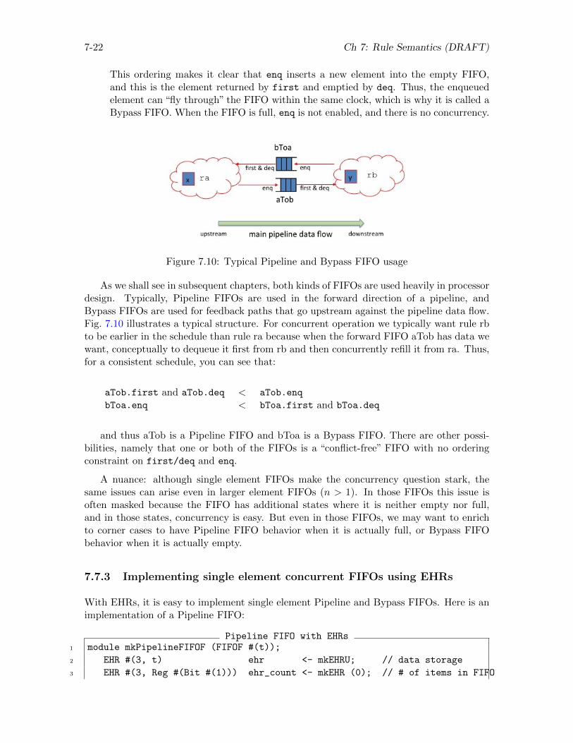
7-22 Ch 7: Rule Semantics (DRAFT)
This ordering makes it clear that enq inserts a new element into the empty FIFO,and this is the element returned by first and emptied by deq. Thus, the enqueuedelement can “fly through” the FIFO within the same clock, which is why it is called aBypass FIFO. When the FIFO is full, enq is not enabled, and there is no concurrency.
Figure 7.10: Typical Pipeline and Bypass FIFO usage
As we shall see in subsequent chapters, both kinds of FIFOs are used heavily in processordesign. Typically, Pipeline FIFOs are used in the forward direction of a pipeline, andBypass FIFOs are used for feedback paths that go upstream against the pipeline data flow.Fig. 7.10 illustrates a typical structure. For concurrent operation we typically want rule rbto be earlier in the schedule than rule ra because when the forward FIFO aTob has data wewant, conceptually to dequeue it first from rb and then concurrently refill it from ra. Thus,for a consistent schedule, you can see that:
aTob.first and aTob.deq < aTob.enq
bToa.enq < bToa.first and bToa.deq
and thus aTob is a Pipeline FIFO and bToa is a Bypass FIFO. There are other possi-bilities, namely that one or both of the FIFOs is a “conflict-free” FIFO with no orderingconstraint on first/deq and enq.
A nuance: although single element FIFOs make the concurrency question stark, thesame issues can arise even in larger element FIFOs (n > 1). In those FIFOs this issue isoften masked because the FIFO has additional states where it is neither empty nor full,and in those states, concurrency is easy. But even in those FIFOs, we may want to enrichto corner cases to have Pipeline FIFO behavior when it is actually full, or Bypass FIFObehavior when it is actually empty.
7.7.3 Implementing single element concurrent FIFOs using EHRs
With EHRs, it is easy to implement single element Pipeline and Bypass FIFOs. Here is animplementation of a Pipeline FIFO:
Pipeline FIFO with EHRs1 module mkPipelineFIFOF (FIFOF #(t));
2 EHR #(3, t) ehr <- mkEHRU; // data storage
3 EHR #(3, Reg #(Bit #(1))) ehr_count <- mkEHR (0); // # of items in FIFO
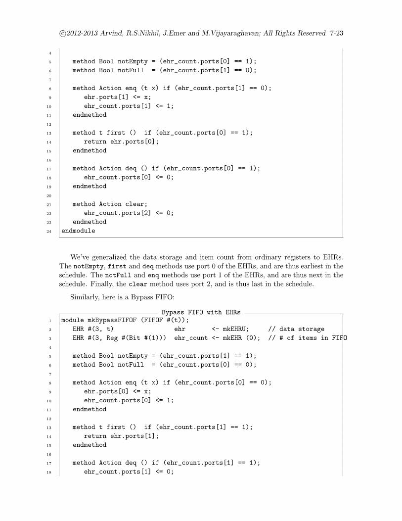
c©2012-2013 Arvind, R.S.Nikhil, J.Emer and M.Vijayaraghavan; All Rights Reserved 7-23
4
5 method Bool notEmpty = (ehr_count.ports[0] == 1);
6 method Bool notFull = (ehr_count.ports[1] == 0);
7
8 method Action enq (t x) if (ehr_count.ports[1] == 0);
9 ehr.ports[1] <= x;
10 ehr_count.ports[1] <= 1;
11 endmethod
12
13 method t first () if (ehr_count.ports[0] == 1);
14 return ehr.ports[0];
15 endmethod
16
17 method Action deq () if (ehr_count.ports[0] == 1);
18 ehr_count.ports[0] <= 0;
19 endmethod
20
21 method Action clear;
22 ehr_count.ports[2] <= 0;
23 endmethod
24 endmodule
We’ve generalized the data storage and item count from ordinary registers to EHRs.The notEmpty, first and deq methods use port 0 of the EHRs, and are thus earliest in theschedule. The notFull and enq methods use port 1 of the EHRs, and are thus next in theschedule. Finally, the clear method uses port 2, and is thus last in the schedule.
Similarly, here is a Bypass FIFO:
Bypass FIFO with EHRs1 module mkBypassFIFOF (FIFOF #(t));
2 EHR #(3, t) ehr <- mkEHRU; // data storage
3 EHR #(3, Reg #(Bit #(1))) ehr_count <- mkEHR (0); // # of items in FIFO
4
5 method Bool notEmpty = (ehr_count.ports[1] == 1);
6 method Bool notFull = (ehr_count.ports[0] == 0);
7
8 method Action enq (t x) if (ehr_count.ports[0] == 0);
9 ehr.ports[0] <= x;
10 ehr_count.ports[0] <= 1;
11 endmethod
12
13 method t first () if (ehr_count.ports[1] == 1);
14 return ehr.ports[1];
15 endmethod
16
17 method Action deq () if (ehr_count.ports[1] == 1);
18 ehr_count.ports[1] <= 0;
7-24 Ch 7: Rule Semantics (DRAFT)
19 endmethod
20
21 method Action clear;
22 ehr_count.ports[2] <= 0;
23 endmethod
24 endmodule
Here we have just reversed the port assignments compared to the Pipeline FIFO: notFulland enq use port 0 and are thus earliest in the schedule; notEmpty, first and deq use port1 and are next in the schedule; and clear, as before, used port 2 and is last in the schedule.
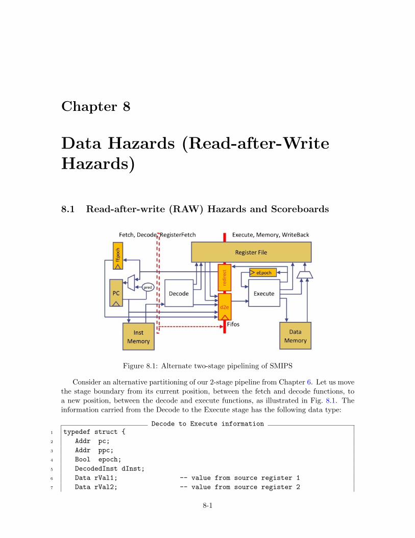
Chapter 8
Data Hazards (Read-after-WriteHazards)
8.1 Read-after-write (RAW) Hazards and Scoreboards
Figure 8.1: Alternate two-stage pipelining of SMIPS
Consider an alternative partitioning of our 2-stage pipeline from Chapter 6. Let us movethe stage boundary from its current position, between the fetch and decode functions, toa new position, between the decode and execute functions, as illustrated in Fig. 8.1. Theinformation carried from the Decode to the Execute stage has the following data type:
Decode to Execute information1 typedef struct {
2 Addr pc;
3 Addr ppc;
4 Bool epoch;
5 DecodedInst dInst;
6 Data rVal1; -- value from source register 1
7 Data rVal2; -- value from source register 2
8-1
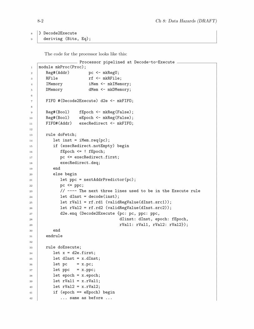
8-2 Ch 8: Data Hazards (DRAFT)
8 } Decode2Execute
9 deriving (Bits, Eq);
The code for the processor looks like this:
Processor pipelined at Decode-to-Execute1 module mkProc(Proc);
2 Reg#(Addr) pc <- mkRegU;
3 RFile rf <- mkRFile;
4 IMemory iMem <- mkIMemory;
5 DMemory dMem <- mkDMemory;
6
7 FIFO #(Decode2Execute) d2e <- mkFIFO;
8
9 Reg#(Bool) fEpoch <- mkReg(False);
10 Reg#(Bool) eEpoch <- mkReg(False);
11 FIFO#(Addr) execRedirect <- mkFIFO;
12
13 rule doFetch;
14 let inst = iMem.req(pc);
15 if (execRedirect.notEmpty) begin
16 fEpoch <= ! fEpoch;
17 pc <= execRedirect.first;
18 execRedirect.deq;
19 end
20 else begin
21 let ppc = nextAddrPredictor(pc);
22 pc <= ppc;
23 // ---- The next three lines used to be in the Execute rule
24 let dInst = decode(inst);
25 let rVal1 = rf.rd1 (validRegValue(dInst.src1));
26 let rVal2 = rf.rd2 (validRegValue(dInst.src2));
27 d2e.enq (Decode2Execute {pc: pc, ppc: ppc,
28 dIinst: dInst, epoch: fEpoch,
29 rVal1: rVal1, rVal2: rVal2});
30 end
31 endrule
32
33 rule doExecute;
34 let x = d2e.first;
35 let dInst = x.dInst;
36 let pc = x.pc;
37 let ppc = x.ppc;
38 let epoch = x.epoch;
39 let rVal1 = x.rVal1;
40 let rVal2 = x.rVal2;
41 if (epoch == eEpoch) begin
42 ... same as before ...
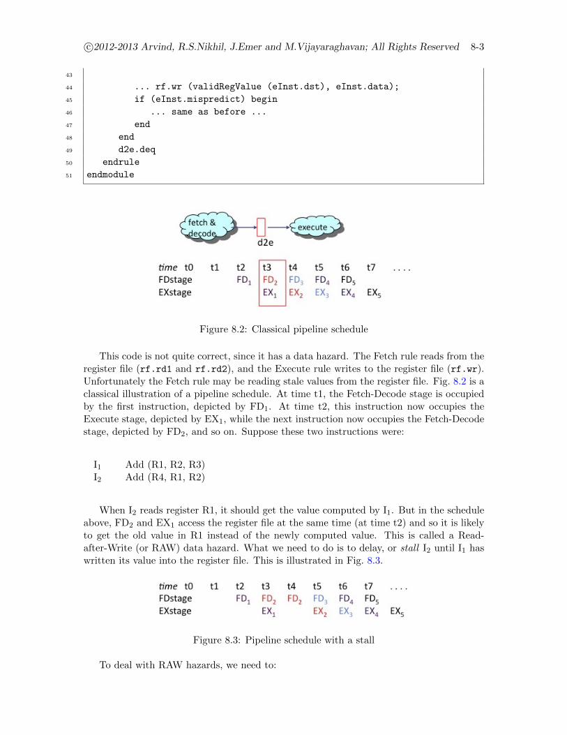
c©2012-2013 Arvind, R.S.Nikhil, J.Emer and M.Vijayaraghavan; All Rights Reserved 8-3
43
44 ... rf.wr (validRegValue (eInst.dst), eInst.data);
45 if (eInst.mispredict) begin
46 ... same as before ...
47 end
48 end
49 d2e.deq
50 endrule
51 endmodule
Figure 8.2: Classical pipeline schedule
This code is not quite correct, since it has a data hazard. The Fetch rule reads from theregister file (rf.rd1 and rf.rd2), and the Execute rule writes to the register file (rf.wr).Unfortunately the Fetch rule may be reading stale values from the register file. Fig. 8.2 is aclassical illustration of a pipeline schedule. At time t1, the Fetch-Decode stage is occupiedby the first instruction, depicted by FD1. At time t2, this instruction now occupies theExecute stage, depicted by EX1, while the next instruction now occupies the Fetch-Decodestage, depicted by FD2, and so on. Suppose these two instructions were:
I1 Add (R1, R2, R3)I2 Add (R4, R1, R2)
When I2 reads register R1, it should get the value computed by I1. But in the scheduleabove, FD2 and EX1 access the register file at the same time (at time t2) and so it is likelyto get the old value in R1 instead of the newly computed value. This is called a Read-after-Write (or RAW) data hazard. What we need to do is to delay, or stall I2 until I1 haswritten its value into the register file. This is illustrated in Fig. 8.3.
Figure 8.3: Pipeline schedule with a stall
To deal with RAW hazards, we need to:
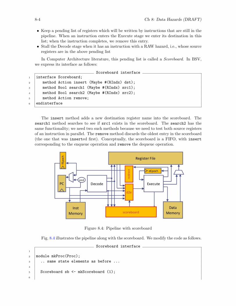
8-4 Ch 8: Data Hazards (DRAFT)
• Keep a pending list of registers which will be written by instructions that are still in thepipeline. When an instruction enters the Execute stage we enter its destination in thislist; when the instruction completes, we remove this entry.• Stall the Decode stage when it has an instruction with a RAW hazard, i.e., whose source
registers are in the above pending list
In Computer Architecture literature, this pending list is called a Scoreboard. In BSV,we express its interface as follows:
Scoreboard interface1 interface Scoreboard;
2 method Action insert (Maybe #(RIndx) dst);
3 method Bool search1 (Maybe #(RIndx) src1);
4 method Bool search2 (Maybe #(RIndx) src2);
5 method Action remove;
6 endinterface
The insert method adds a new destination register name into the scoreboard. Thesearch1 method searches to see if src1 exists in the scoreboard. The search2 has thesame functionality; we need two such methods because we need to test both source registersof an instruction in parallel. The remove method discards the oldest entry in the scoreboard(the one that was inserted first). Conceptually, the scoreboard is a FIFO, with insert
corresponding to the enqueue operation and remove the dequeue operation.
Figure 8.4: Pipeline with scoreboard
Fig. 8.4 illustrates the pipeline along with the scoreboard. We modify the code as follows.
Scoreboard interface1
2 module mkProc(Proc);
3 .. same state elements as before ...
4
5 Scoreboard sb <- mkScoreboard (1);
6
c©2012-2013 Arvind, R.S.Nikhil, J.Emer and M.Vijayaraghavan; All Rights Reserved 8-5
7 rule doFetch;
8 let inst = iMem.req(pc);
9 if (execRedirect.notEmpty) begin
10 ... seame as before ...
11 end
12 else begin
13 let ppc = nextAddrPredictor (pc);
14 let dInst = decode(inst);
15 let stall = sb.search1 (dInst.src1) || sb.search2 (dInst.src2);
16 if (! stall) begin
17 let rVal1 = rf.rd1 (validRegValue(dInst.src1));
18 let rVal2 = rf.rd2 (validRegValue(dInst.src2));
19 d2e.enq(Decode2Execute {pc: pc, ppc: ppc,
20 dIinst: dInst, epoch: fEpoch,
21 rVal1: rVal1, rVal2: rVal2});
22 sb.insert(dInst.rDst);
23 pc <= ppc;
24 end
25 end
26 endrule
27
28 rule doExecute;
29 let x = d2e.first;
30 ... same as before ...
31 if (epoch == eEpoch) begin
32 ... same execution as before ...
33 end
34 d2e.deq;
35 sb.remove;
36 endrule
37 endmodule
In line 5 we instantiate a scoreboard with size 1 (holds one entry). This is because,in this pipeline, there is at most one pending instruction in the Execute stage. In line 15we search the scoreboard for data hazards; we perform the register reads and forward theinstruction in the following lines only if we do not stall. In line 22 we insert the destinationregister of the current instruction into the scoreboard. Note that line 23 updates the PConly if we do not stall; if we stall, this rule will be repeated at the same PC. In the Executerule, the only difference is that, in line 35, we remove the completed instruction’s destinationregister from the scoreboard.
We invoke search1, search2 and insert in a single rule (doFetch), i.e., at a singleinstant. Clearly, we expect the single-rule semantics of these methods to be such that thesearches check the existing state of the scoreboard (due to previous instructions only), andinsert creates the next state of the scoreboard. There is no concurrency issue here sincethey are invoked in the same rule.
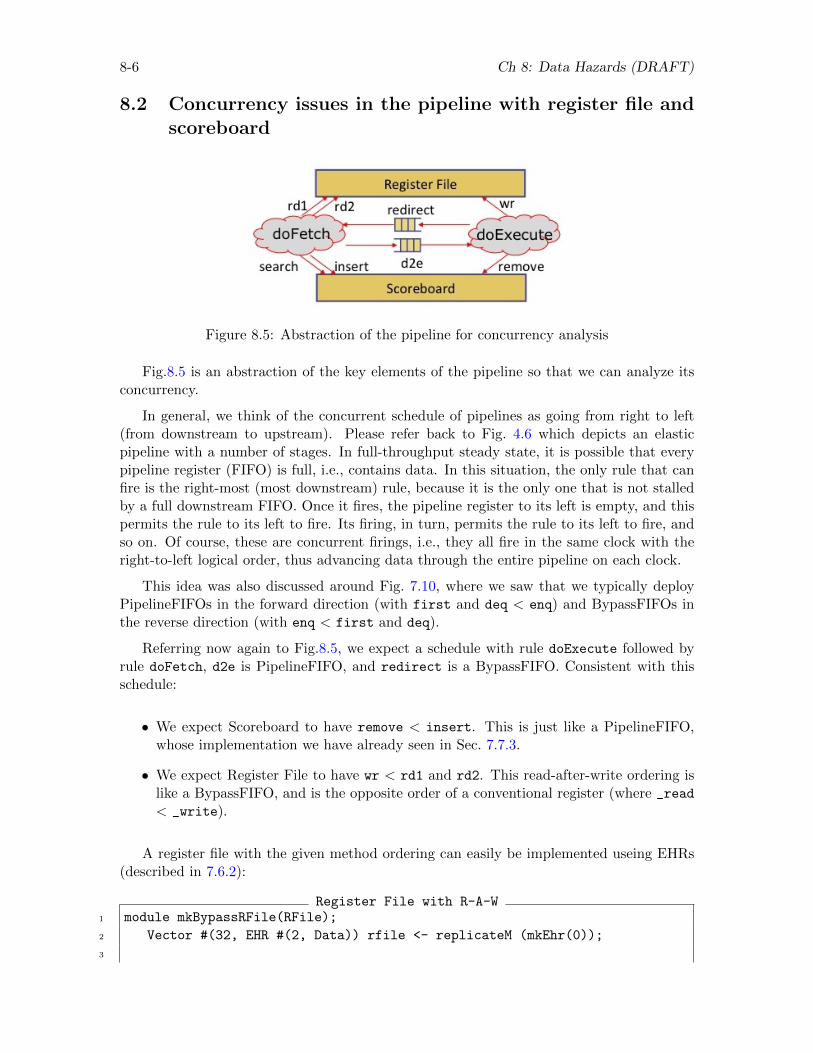
8-6 Ch 8: Data Hazards (DRAFT)
8.2 Concurrency issues in the pipeline with register file andscoreboard
Figure 8.5: Abstraction of the pipeline for concurrency analysis
Fig.8.5 is an abstraction of the key elements of the pipeline so that we can analyze itsconcurrency.
In general, we think of the concurrent schedule of pipelines as going from right to left(from downstream to upstream). Please refer back to Fig. 4.6 which depicts an elasticpipeline with a number of stages. In full-throughput steady state, it is possible that everypipeline register (FIFO) is full, i.e., contains data. In this situation, the only rule that canfire is the right-most (most downstream) rule, because it is the only one that is not stalledby a full downstream FIFO. Once it fires, the pipeline register to its left is empty, and thispermits the rule to its left to fire. Its firing, in turn, permits the rule to its left to fire, andso on. Of course, these are concurrent firings, i.e., they all fire in the same clock with theright-to-left logical order, thus advancing data through the entire pipeline on each clock.
This idea was also discussed around Fig. 7.10, where we saw that we typically deployPipelineFIFOs in the forward direction (with first and deq < enq) and BypassFIFOs inthe reverse direction (with enq < first and deq).
Referring now again to Fig.8.5, we expect a schedule with rule doExecute followed byrule doFetch, d2e is PipelineFIFO, and redirect is a BypassFIFO. Consistent with thisschedule:
• We expect Scoreboard to have remove < insert. This is just like a PipelineFIFO,whose implementation we have already seen in Sec. 7.7.3.
• We expect Register File to have wr < rd1 and rd2. This read-after-write ordering islike a BypassFIFO, and is the opposite order of a conventional register (where _read
< _write).
A register file with the given method ordering can easily be implemented useing EHRs(described in 7.6.2):
Register File with R-A-W1 module mkBypassRFile(RFile);
2 Vector #(32, EHR #(2, Data)) rfile <- replicateM (mkEhr(0));
3
c©2012-2013 Arvind, R.S.Nikhil, J.Emer and M.Vijayaraghavan; All Rights Reserved 8-7
4 method Action wr(RIndx rindx, Data data);
5 if (rindex!==0)
6 (rfile[rindex])[0] <= data;
7 endmethod
8
9 method Data rd1 (RIndx rindx) = (rfile[rindx])[1];
10
11 method Data rd2 (RIndx rindx) = (rfile[rindx])[1];
12 endmodule
8.3 Write-after-Write Hazards
What happens if a fetched instruction has no RAW hazards, but writes to the same registeras an instruction that is still in the pipeline? This is called a Write-after-Write (WAW)hazard. Note, there can be no instruction ahead of it that reads that register, since anyinstruction would still be stalled in the Fetch stage.
There are two ways we could solve this problem:
1. If we implement our scoreboard as a FIFO, there is no problem. The current instruc-tion will be enqueued into the scoreboard, which may now contain two identical entries.Any later instruction that reads this register will be stalled until both correspondingwriting instructions have completed and these entries have been removed.
2. We could implement the scoreboard as a simple bit vector with one bit per registerin the register file. The insert method sets a bit, and the remove method resets it.In this case, since we can’t keep track of multiple instructions writing to the sameregister, we must stall any instruction that has a WAW hazard. This will requireanother search3 method to test the destination register of an instruction in additionto its sources, in the Decode logic.
8.4 Deeper pipelines
Fig. 8.6 illustrates a version of our pipeline that is partitioned into 3 stages. The previousExecute stage has been refined into two parts, one that performs the ALU and memoryoperations and another, the“Commit”stage, that performs the writeback of the output valueto the register file (if the instruction has an output). Since there can now be two instructions“in flight” ahead of the Decode stage, we need to increase the size of the scoreboard to holdtwo destination register names.
In the Execute stage, when we kill a wrong-path instruction, we can pass an “Invalid”destination to the Commit stage, like so:
Execute stage in 3-stage pipeline1 rule doExecute;
2 ... same as before ...
3 if (epoch == eEpoch) begin
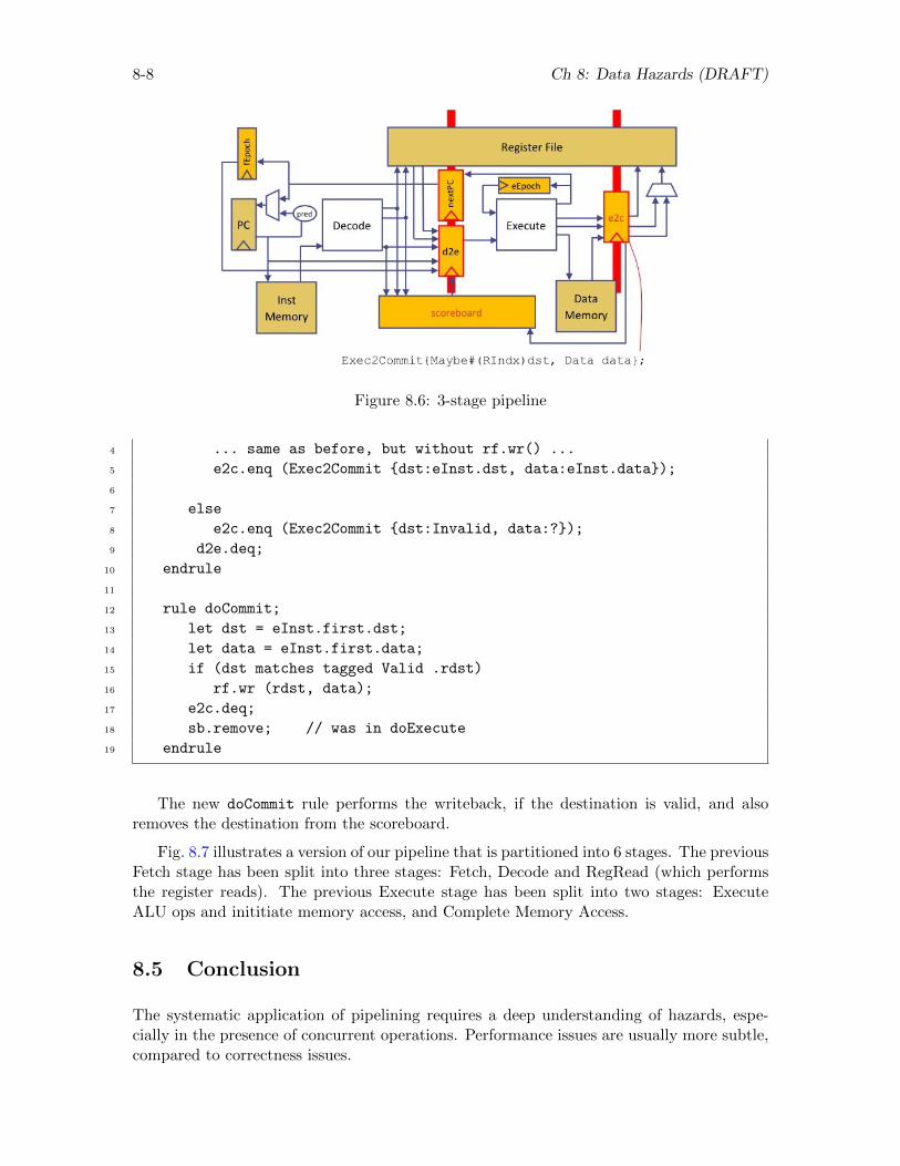
8-8 Ch 8: Data Hazards (DRAFT)
Figure 8.6: 3-stage pipeline
4 ... same as before, but without rf.wr() ...
5 e2c.enq (Exec2Commit {dst:eInst.dst, data:eInst.data});
6
7 else
8 e2c.enq (Exec2Commit {dst:Invalid, data:?});
9 d2e.deq;
10 endrule
11
12 rule doCommit;
13 let dst = eInst.first.dst;
14 let data = eInst.first.data;
15 if (dst matches tagged Valid .rdst)
16 rf.wr (rdst, data);
17 e2c.deq;
18 sb.remove; // was in doExecute
19 endrule
The new doCommit rule performs the writeback, if the destination is valid, and alsoremoves the destination from the scoreboard.
Fig. 8.7 illustrates a version of our pipeline that is partitioned into 6 stages. The previousFetch stage has been split into three stages: Fetch, Decode and RegRead (which performsthe register reads). The previous Execute stage has been split into two stages: ExecuteALU ops and inititiate memory access, and Complete Memory Access.
8.5 Conclusion
The systematic application of pipelining requires a deep understanding of hazards, espe-cially in the presence of concurrent operations. Performance issues are usually more subtle,compared to correctness issues.
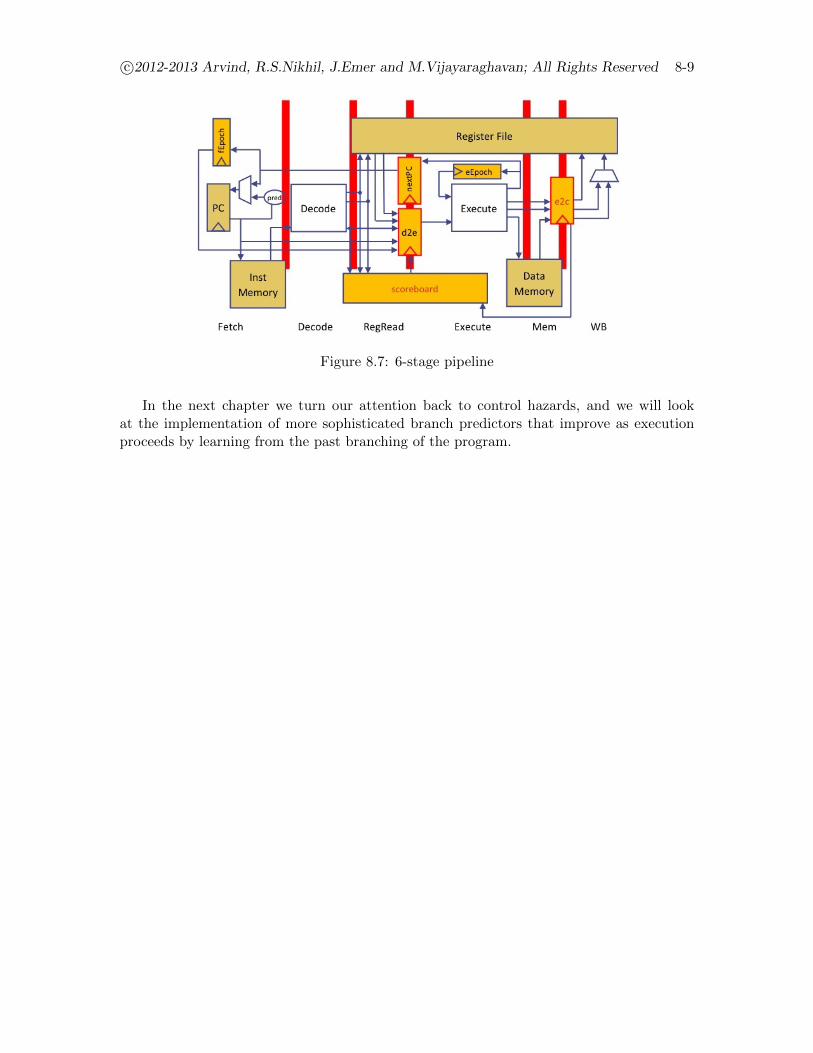
c©2012-2013 Arvind, R.S.Nikhil, J.Emer and M.Vijayaraghavan; All Rights Reserved 8-9
Figure 8.7: 6-stage pipeline
In the next chapter we turn our attention back to control hazards, and we will lookat the implementation of more sophisticated branch predictors that improve as executionproceeds by learning from the past branching of the program.

8-10 Ch 8: Data Hazards (DRAFT)
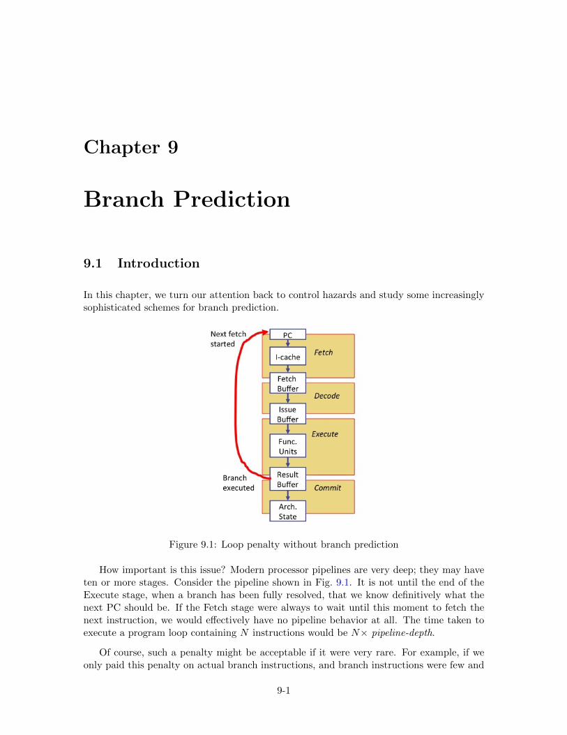
Chapter 9
Branch Prediction
9.1 Introduction
In this chapter, we turn our attention back to control hazards and study some increasinglysophisticated schemes for branch prediction.
Figure 9.1: Loop penalty without branch prediction
How important is this issue? Modern processor pipelines are very deep; they may haveten or more stages. Consider the pipeline shown in Fig. 9.1. It is not until the end of theExecute stage, when a branch has been fully resolved, that we know definitively what thenext PC should be. If the Fetch stage were always to wait until this moment to fetch thenext instruction, we would effectively have no pipeline behavior at all. The time taken toexecute a program loop containing N instructions would be N× pipeline-depth.
Of course, such a penalty might be acceptable if it were very rare. For example, if weonly paid this penalty on actual branch instructions, and branch instructions were few and
9-1
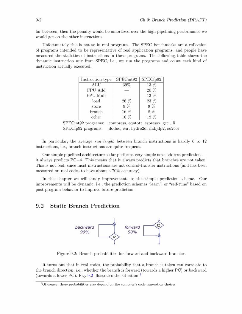
9-2 Ch 9: Branch Prediction (DRAFT)
far between, then the penalty would be amortized over the high pipelining performance wewould get on the other instructions.
Unfortunately this is not so in real programs. The SPEC benchmarks are a collectionof programs intended to be representative of real application programs, and people havemeasured the statistics of instructions in these programs. The following table shows thedynamic instruction mix from SPEC, i.e., we run the programs and count each kind ofinstruction actually executed.
Instruction type SPECint92 SPECfp92
ALU 39% 13 %FPU Add — 20 %FPU Mult — 13 %
load 26 % 23 %store 9 % 9 %
branch 16 % 8 %other 10 % 12 %
SPECint92 programs: compress, eqntott, espresso, gcc , liSPECfp92 programs: doduc, ear, hydro2d, mdijdp2, su2cor
In particular, the average run length between branch instructions is hardly 6 to 12instructions, i.e., branch instructions are quite frequent.
Our simple pipelined architecture so far performs very simple next-address predictions—it always predicts PC+4. This means that it always predicts that branches are not taken.This is not bad, since most instructions are not control-transfer instructions (and has beenmeasured on real codes to have about a 70% accuracy).
In this chapter we will study improvements to this simple prediction scheme. Ourimprovements will be dynamic, i.e., the prediction schemes “learn”, or “self-tune” based onpast program behavior to improve future prediction.
9.2 Static Branch Prediction
Figure 9.2: Branch probabilities for forward and backward branches
It turns out that in real codes, the probability that a branch is taken can correlate tothe branch direction, i.e., whether the branch is forward (towards a higher PC) or backward(towards a lower PC). Fig. 9.2 illustrates the situation.1
1Of course, these probabilities also depend on the compiler’s code generation choices.
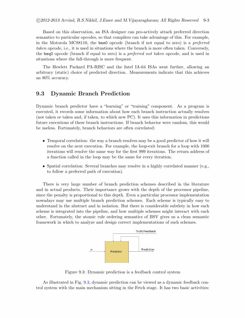
c©2012-2013 Arvind, R.S.Nikhil, J.Emer and M.Vijayaraghavan; All Rights Reserved 9-3
Based on this observation, an ISA designer can pro-actively attach preferred directionsemantics to particular opcodes, so that compilers can take advantage of this. For example,in the Motorola MC88110, the bne0 opcode (branch if not equal to zero) is a preferredtaken opcode, i.e., it is used in situations where the branch is more often taken. Conversely,the beq0 opcode (branch if equal to zero) is a preferred not taken opcode, and is used insituations where the fall-through is more frequent.
The Hewlett Packard PA-RISC and the Intel IA-64 ISAs went further, allowing anarbitrary (static) choice of predicted direction. Measurements indicate that this achievesan 80% accuracy.
9.3 Dynamic Branch Prediction
Dynamic branch predictor have a “learning” or “training” component. As a program isexecuted, it records some information about how each branch instruction actually resolves(not taken or taken and, if taken, to which new PC). It uses this information in predictionsfuture executions of these branch instructions. If branch behavior were random, this wouldbe useless. Fortunately, branch behaviors are often correlated:
• Temporal correlation: the way a branch resolves may be a good predictor of how it willresolve on the next execution. For example, the loop-exit branch for a loop with 1000iterations will resolve the same way for the first 999 iterations. The return address ofa function called in the loop may be the same for every iteration.
• Spatial correlation: Several branches may resolve in a highly correlated manner (e.g.,to follow a preferred path of execution).
There is very large number of branch prediction schemes described in the literatureand in actual products. Their importance grows with the depth of the processor pipeline,since the penalty is proportional to this depth. Even a particular processor implementationnowadays may use multiple branch prediction schemes. Each scheme is typically easy tounderstand in the abstract and in isolation. But there is considerable subtlety in how eachscheme is integrated into the pipeline, and how multiple schemes might interact with eachother. Fortunately, the atomic rule ordering semantics of BSV gives us a clean semanticframework in which to analyze and design correct implementations of such schemes.
Figure 9.3: Dynamic prediction is a feedback control system
As illustrated in Fig. 9.3, dynamic prediction can be viewed as a dynamic feedback con-trol system with the main mechanism sitting in the Fetch stage. It has two basic activities:
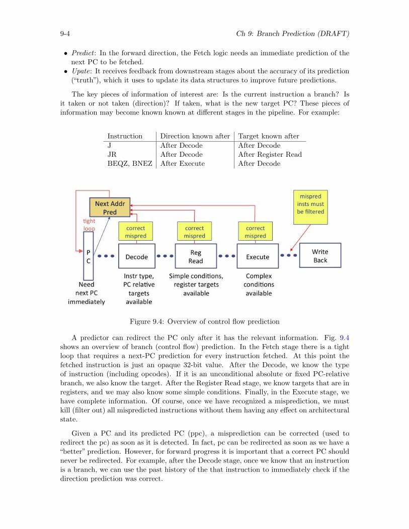
9-4 Ch 9: Branch Prediction (DRAFT)
• Predict : In the forward direction, the Fetch logic needs an immediate prediction of thenext PC to be fetched.• Upate: It receives feedback from downstream stages about the accuracy of its prediction
(“truth”), which it uses to update its data structures to improve future predictions.
The key pieces of information of interest are: Is the current instruction a branch? Isit taken or not taken (direction)? If taken, what is the new target PC? These pieces ofinformation may become known known at different stages in the pipeline. For example:
Instruction Direction known after Target known after
J After Decode After DecodeJR After Decode After Register ReadBEQZ, BNEZ After Execute After Decode
Figure 9.4: Overview of control flow prediction
A predictor can redirect the PC only after it has the relevant information. Fig. 9.4shows an overview of branch (control flow) prediction. In the Fetch stage there is a tightloop that requires a next-PC prediction for every instruction fetched. At this point thefetched instruction is just an opaque 32-bit value. After the Decode, we know the typeof instruction (including opcodes). If it is an unconditional absolute or fixed PC-relativebranch, we also know the target. After the Register Read stage, we know targets that are inregisters, and we may also know some simple conditions. Finally, in the Execute stage, wehave complete information. Of course, once we have recognized a misprediction, we mustkill (filter out) all mispredicted instructions without them having any effect on architecturalstate.
Given a PC and its predicted PC (ppc), a misprediction can be corrected (used toredirect the pc) as soon as it is detected. In fact, pc can be redirected as soon as we have a“better” prediction. However, for forward progress it is important that a correct PC shouldnever be redirected. For example, after the Decode stage, once we know that an instructionis a branch, we can use the past history of the that instruction to immediately check if thedirection prediction was correct.
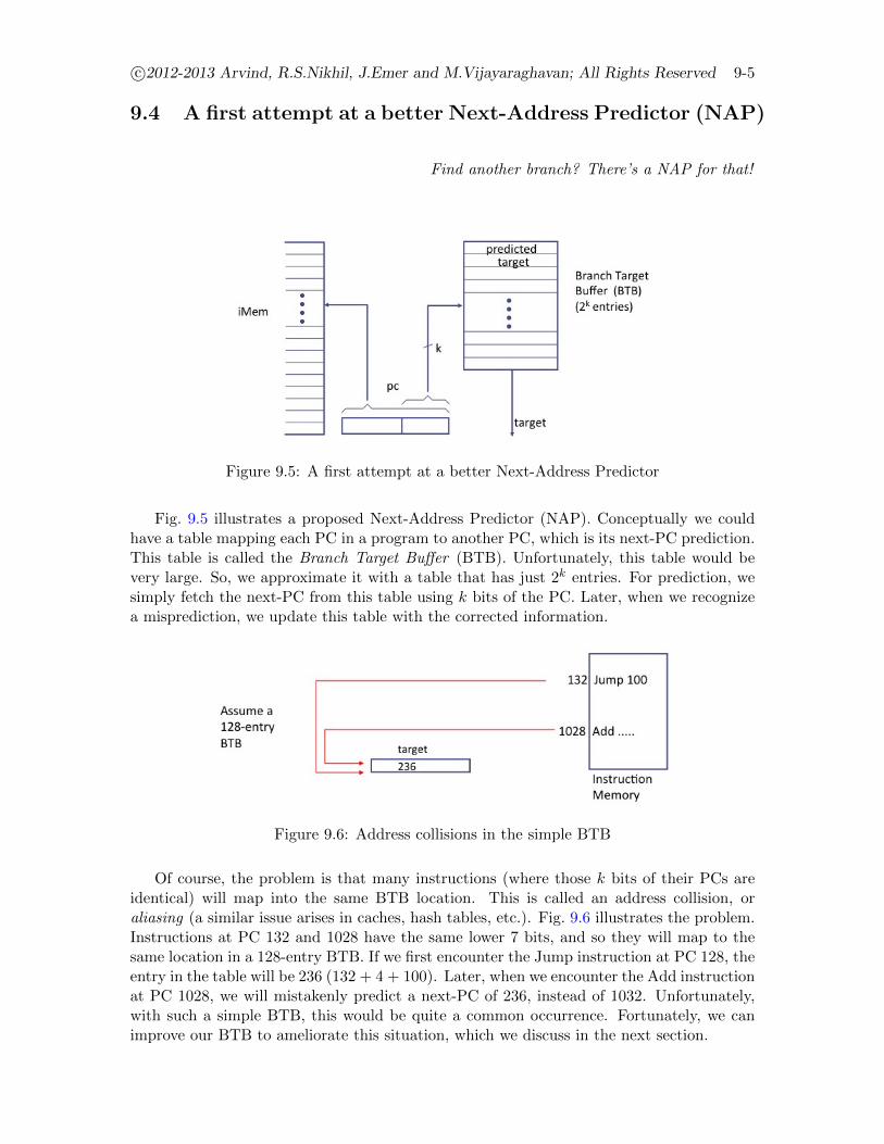
c©2012-2013 Arvind, R.S.Nikhil, J.Emer and M.Vijayaraghavan; All Rights Reserved 9-5
9.4 A first attempt at a better Next-Address Predictor (NAP)
Find another branch? There’s a NAP for that!
Figure 9.5: A first attempt at a better Next-Address Predictor
Fig. 9.5 illustrates a proposed Next-Address Predictor (NAP). Conceptually we couldhave a table mapping each PC in a program to another PC, which is its next-PC prediction.This table is called the Branch Target Buffer (BTB). Unfortunately, this table would bevery large. So, we approximate it with a table that has just 2k entries. For prediction, wesimply fetch the next-PC from this table using k bits of the PC. Later, when we recognizea misprediction, we update this table with the corrected information.
Figure 9.6: Address collisions in the simple BTB
Of course, the problem is that many instructions (where those k bits of their PCs areidentical) will map into the same BTB location. This is called an address collision, oraliasing (a similar issue arises in caches, hash tables, etc.). Fig. 9.6 illustrates the problem.Instructions at PC 132 and 1028 have the same lower 7 bits, and so they will map to thesame location in a 128-entry BTB. If we first encounter the Jump instruction at PC 128, theentry in the table will be 236 (132 + 4 + 100). Later, when we encounter the Add instructionat PC 1028, we will mistakenly predict a next-PC of 236, instead of 1032. Unfortunately,with such a simple BTB, this would be quite a common occurrence. Fortunately, we canimprove our BTB to ameliorate this situation, which we discuss in the next section.
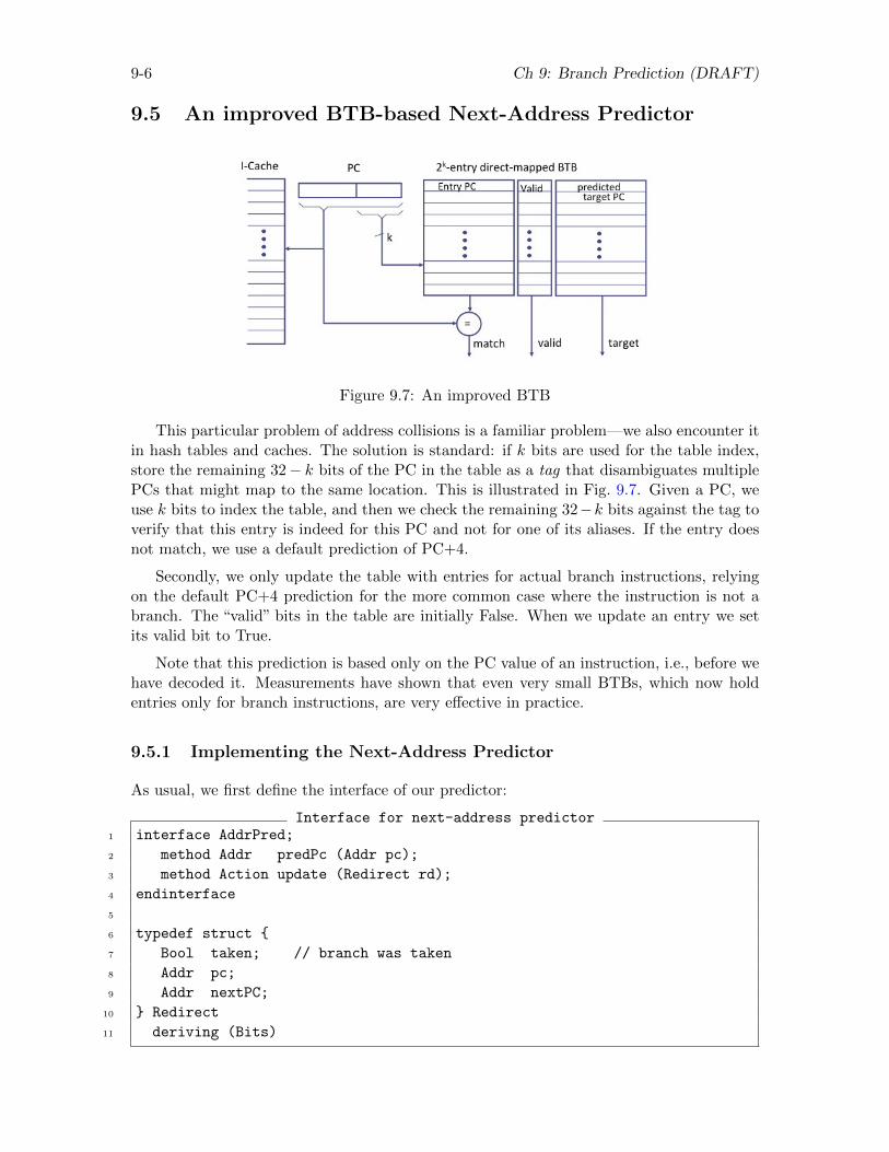
9-6 Ch 9: Branch Prediction (DRAFT)
9.5 An improved BTB-based Next-Address Predictor
Figure 9.7: An improved BTB
This particular problem of address collisions is a familiar problem—we also encounter itin hash tables and caches. The solution is standard: if k bits are used for the table index,store the remaining 32− k bits of the PC in the table as a tag that disambiguates multiplePCs that might map to the same location. This is illustrated in Fig. 9.7. Given a PC, weuse k bits to index the table, and then we check the remaining 32−k bits against the tag toverify that this entry is indeed for this PC and not for one of its aliases. If the entry doesnot match, we use a default prediction of PC+4.
Secondly, we only update the table with entries for actual branch instructions, relyingon the default PC+4 prediction for the more common case where the instruction is not abranch. The “valid” bits in the table are initially False. When we update an entry we setits valid bit to True.
Note that this prediction is based only on the PC value of an instruction, i.e., before wehave decoded it. Measurements have shown that even very small BTBs, which now holdentries only for branch instructions, are very effective in practice.
9.5.1 Implementing the Next-Address Predictor
As usual, we first define the interface of our predictor:
Interface for next-address predictor1 interface AddrPred;
2 method Addr predPc (Addr pc);
3 method Action update (Redirect rd);
4 endinterface
5
6 typedef struct {
7 Bool taken; // branch was taken
8 Addr pc;
9 Addr nextPC;
10 } Redirect
11 deriving (Bits)
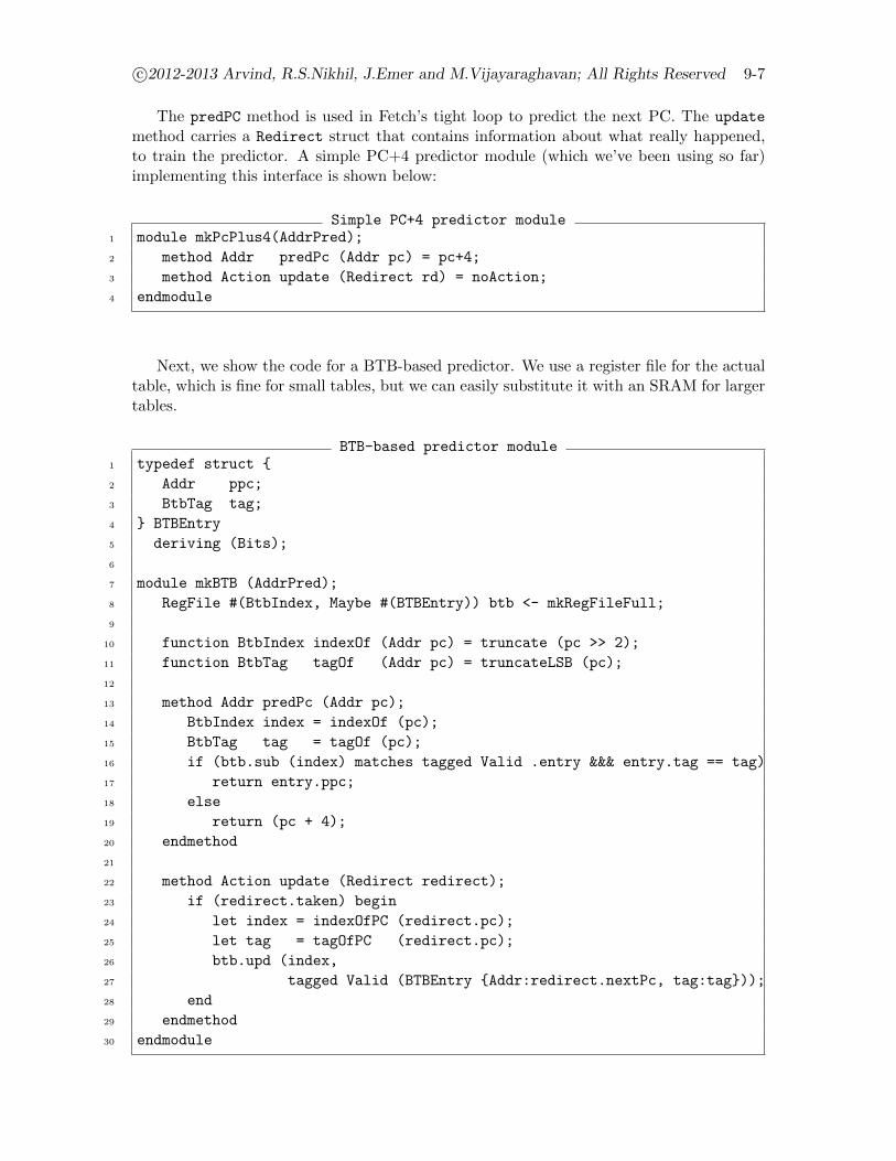
c©2012-2013 Arvind, R.S.Nikhil, J.Emer and M.Vijayaraghavan; All Rights Reserved 9-7
The predPC method is used in Fetch’s tight loop to predict the next PC. The update
method carries a Redirect struct that contains information about what really happened,to train the predictor. A simple PC+4 predictor module (which we’ve been using so far)implementing this interface is shown below:
Simple PC+4 predictor module1 module mkPcPlus4(AddrPred);
2 method Addr predPc (Addr pc) = pc+4;
3 method Action update (Redirect rd) = noAction;
4 endmodule
Next, we show the code for a BTB-based predictor. We use a register file for the actualtable, which is fine for small tables, but we can easily substitute it with an SRAM for largertables.
BTB-based predictor module1 typedef struct {
2 Addr ppc;
3 BtbTag tag;
4 } BTBEntry
5 deriving (Bits);
6
7 module mkBTB (AddrPred);
8 RegFile #(BtbIndex, Maybe #(BTBEntry)) btb <- mkRegFileFull;
9
10 function BtbIndex indexOf (Addr pc) = truncate (pc >> 2);
11 function BtbTag tagOf (Addr pc) = truncateLSB (pc);
12
13 method Addr predPc (Addr pc);
14 BtbIndex index = indexOf (pc);
15 BtbTag tag = tagOf (pc);
16 if (btb.sub (index) matches tagged Valid .entry &&& entry.tag == tag)
17 return entry.ppc;
18 else
19 return (pc + 4);
20 endmethod
21
22 method Action update (Redirect redirect);
23 if (redirect.taken) begin
24 let index = indexOfPC (redirect.pc);
25 let tag = tagOfPC (redirect.pc);
26 btb.upd (index,
27 tagged Valid (BTBEntry {Addr:redirect.nextPc, tag:tag}));
28 end
29 endmethod
30 endmodule
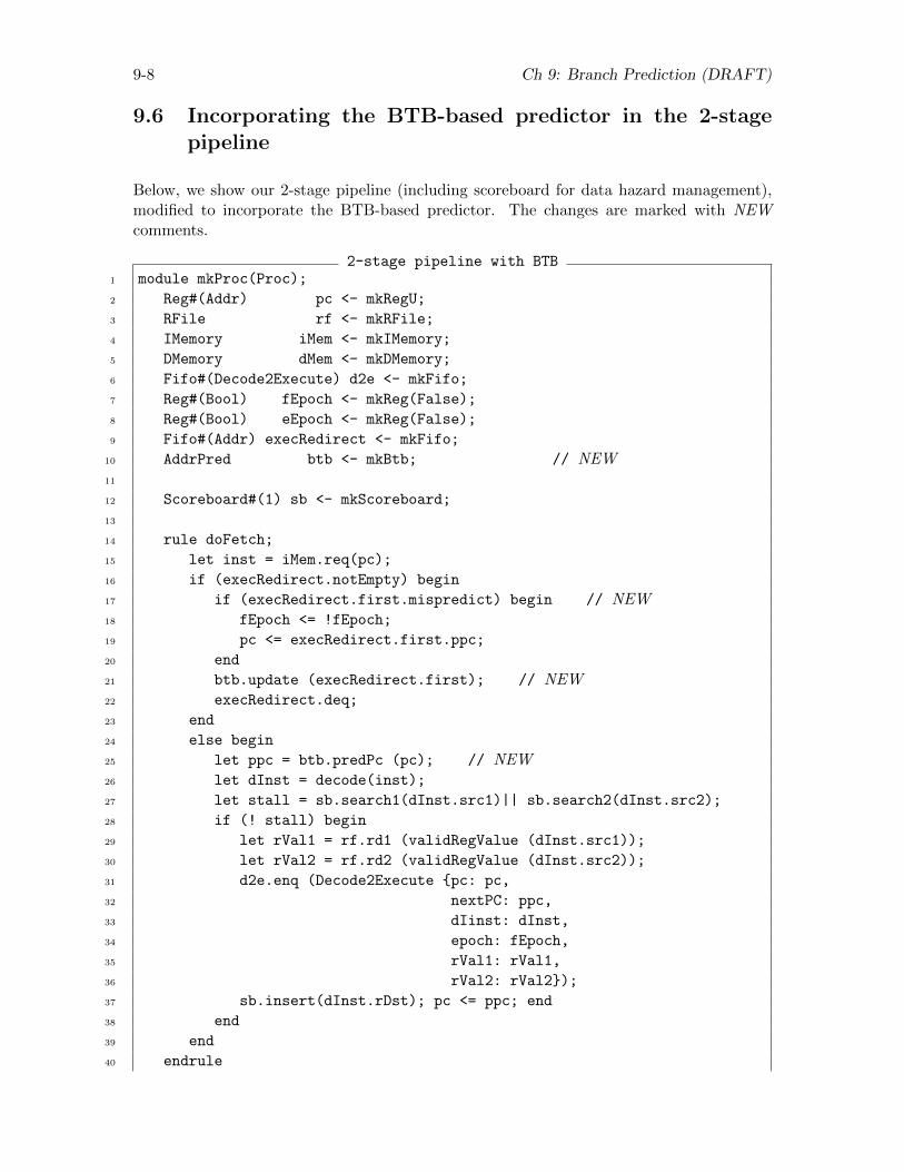
9-8 Ch 9: Branch Prediction (DRAFT)
9.6 Incorporating the BTB-based predictor in the 2-stagepipeline
Below, we show our 2-stage pipeline (including scoreboard for data hazard management),modified to incorporate the BTB-based predictor. The changes are marked with NEWcomments.
2-stage pipeline with BTB1 module mkProc(Proc);
2 Reg#(Addr) pc <- mkRegU;
3 RFile rf <- mkRFile;
4 IMemory iMem <- mkIMemory;
5 DMemory dMem <- mkDMemory;
6 Fifo#(Decode2Execute) d2e <- mkFifo;
7 Reg#(Bool) fEpoch <- mkReg(False);
8 Reg#(Bool) eEpoch <- mkReg(False);
9 Fifo#(Addr) execRedirect <- mkFifo;
10 AddrPred btb <- mkBtb; // NEW11
12 Scoreboard#(1) sb <- mkScoreboard;
13
14 rule doFetch;
15 let inst = iMem.req(pc);
16 if (execRedirect.notEmpty) begin
17 if (execRedirect.first.mispredict) begin // NEW18 fEpoch <= !fEpoch;
19 pc <= execRedirect.first.ppc;
20 end
21 btb.update (execRedirect.first); // NEW22 execRedirect.deq;
23 end
24 else begin
25 let ppc = btb.predPc (pc); // NEW26 let dInst = decode(inst);
27 let stall = sb.search1(dInst.src1)|| sb.search2(dInst.src2);
28 if (! stall) begin
29 let rVal1 = rf.rd1 (validRegValue (dInst.src1));
30 let rVal2 = rf.rd2 (validRegValue (dInst.src2));
31 d2e.enq (Decode2Execute {pc: pc,
32 nextPC: ppc,
33 dIinst: dInst,
34 epoch: fEpoch,
35 rVal1: rVal1,
36 rVal2: rVal2});
37 sb.insert(dInst.rDst); pc <= ppc; end
38 end
39 end
40 endrule
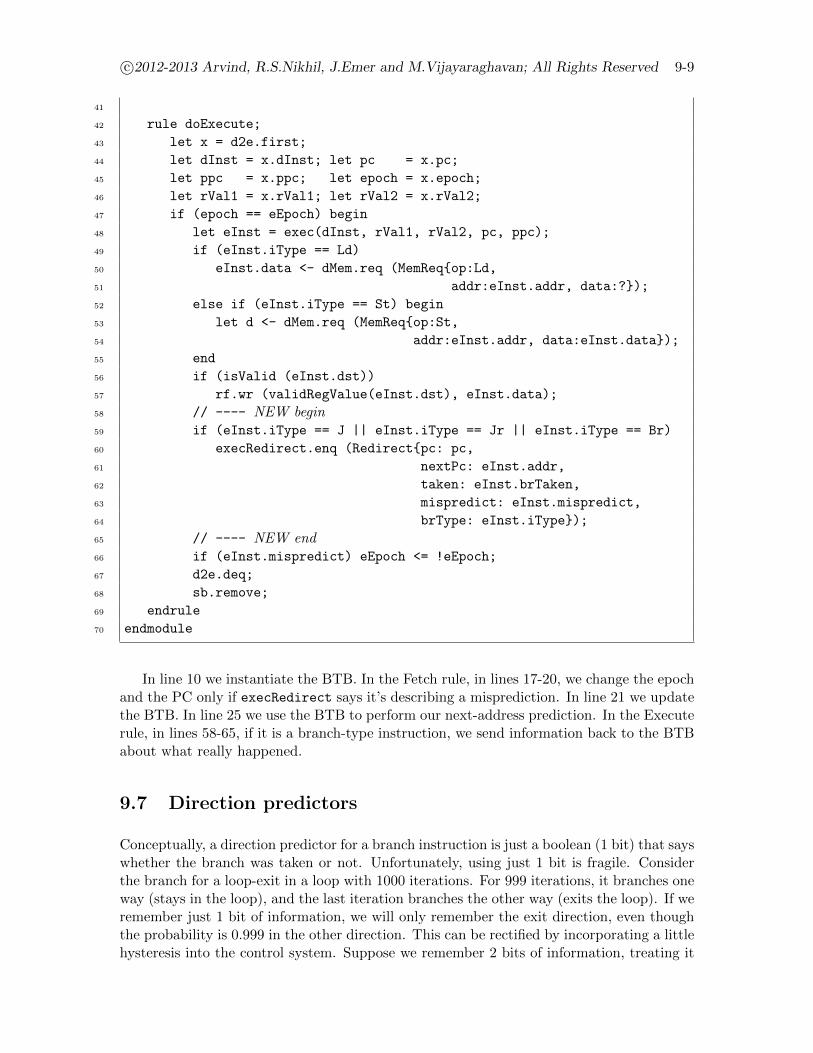
c©2012-2013 Arvind, R.S.Nikhil, J.Emer and M.Vijayaraghavan; All Rights Reserved 9-9
41
42 rule doExecute;
43 let x = d2e.first;
44 let dInst = x.dInst; let pc = x.pc;
45 let ppc = x.ppc; let epoch = x.epoch;
46 let rVal1 = x.rVal1; let rVal2 = x.rVal2;
47 if (epoch == eEpoch) begin
48 let eInst = exec(dInst, rVal1, rVal2, pc, ppc);
49 if (eInst.iType == Ld)
50 eInst.data <- dMem.req (MemReq{op:Ld,
51 addr:eInst.addr, data:?});
52 else if (eInst.iType == St) begin
53 let d <- dMem.req (MemReq{op:St,
54 addr:eInst.addr, data:eInst.data});
55 end
56 if (isValid (eInst.dst))
57 rf.wr (validRegValue(eInst.dst), eInst.data);
58 // ---- NEW begin59 if (eInst.iType == J || eInst.iType == Jr || eInst.iType == Br)
60 execRedirect.enq (Redirect{pc: pc,
61 nextPc: eInst.addr,
62 taken: eInst.brTaken,
63 mispredict: eInst.mispredict,
64 brType: eInst.iType});
65 // ---- NEW end66 if (eInst.mispredict) eEpoch <= !eEpoch;
67 d2e.deq;
68 sb.remove;
69 endrule
70 endmodule
In line 10 we instantiate the BTB. In the Fetch rule, in lines 17-20, we change the epochand the PC only if execRedirect says it’s describing a misprediction. In line 21 we updatethe BTB. In line 25 we use the BTB to perform our next-address prediction. In the Executerule, in lines 58-65, if it is a branch-type instruction, we send information back to the BTBabout what really happened.
9.7 Direction predictors
Conceptually, a direction predictor for a branch instruction is just a boolean (1 bit) that sayswhether the branch was taken or not. Unfortunately, using just 1 bit is fragile. Considerthe branch for a loop-exit in a loop with 1000 iterations. For 999 iterations, it branches oneway (stays in the loop), and the last iteration branches the other way (exits the loop). If weremember just 1 bit of information, we will only remember the exit direction, even thoughthe probability is 0.999 in the other direction. This can be rectified by incorporating a littlehysteresis into the control system. Suppose we remember 2 bits of information, treating it
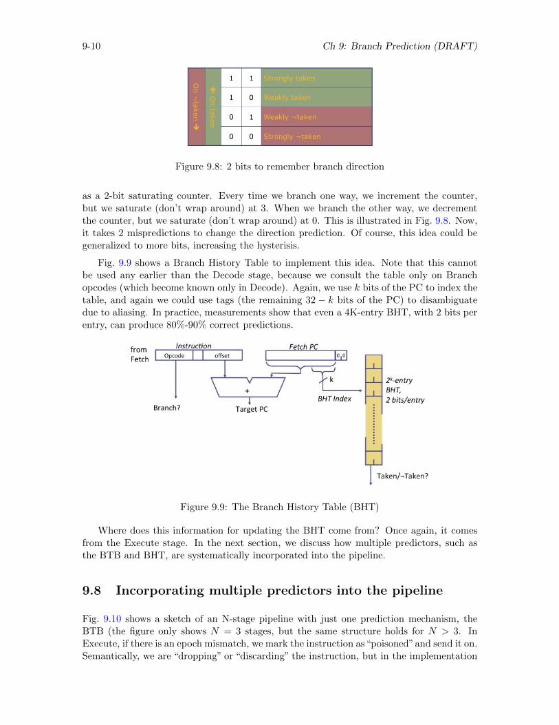
9-10 Ch 9: Branch Prediction (DRAFT)
Figure 9.8: 2 bits to remember branch direction
as a 2-bit saturating counter. Every time we branch one way, we increment the counter,but we saturate (don’t wrap around) at 3. When we branch the other way, we decrementthe counter, but we saturate (don’t wrap around) at 0. This is illustrated in Fig. 9.8. Now,it takes 2 mispredictions to change the direction prediction. Of course, this idea could begeneralized to more bits, increasing the hysterisis.
Fig. 9.9 shows a Branch History Table to implement this idea. Note that this cannotbe used any earlier than the Decode stage, because we consult the table only on Branchopcodes (which become known only in Decode). Again, we use k bits of the PC to index thetable, and again we could use tags (the remaining 32 − k bits of the PC) to disambiguatedue to aliasing. In practice, measurements show that even a 4K-entry BHT, with 2 bits perentry, can produce 80%-90% correct predictions.
Figure 9.9: The Branch History Table (BHT)
Where does this information for updating the BHT come from? Once again, it comesfrom the Execute stage. In the next section, we discuss how multiple predictors, such asthe BTB and BHT, are systematically incorporated into the pipeline.
9.8 Incorporating multiple predictors into the pipeline
Fig. 9.10 shows a sketch of an N-stage pipeline with just one prediction mechanism, theBTB (the figure only shows N = 3 stages, but the same structure holds for N > 3. InExecute, if there is an epoch mismatch, we mark the instruction as“poisoned”and send it on.Semantically, we are “dropping” or “discarding” the instruction, but in the implementation
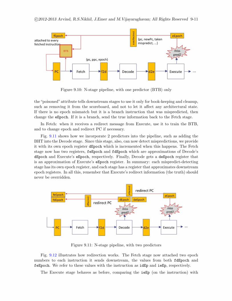
c©2012-2013 Arvind, R.S.Nikhil, J.Emer and M.Vijayaraghavan; All Rights Reserved 9-11
Figure 9.10: N-stage pipeline, with one predictor (BTB) only
the“poisoned”attribute tells downstream stages to use it only for book-keeping and cleanup,such as removing it from the scoreboard, and not to let it affect any architectural state.If there is no epoch mismatch but it is a branch instruction that was mispredicted, thenchange the eEpoch. If it is a branch, send the true information back to the Fetch stage.
In Fetch: when it receives a redirect message from Execute, use it to train the BTB,and to change epoch and redirect PC if necessary.
Fig. 9.11 shows how we incorporate 2 predictors into the pipeline, such as adding theBHT into the Decode stage. Since this stage, also, can now detect mispredictions, we provideit with its own epoch register dEpoch which is incremented when this happens. The Fetchstage now has two registers, feEpoch and fdEpoch which are approximations of Decode’sdEpoch and Execute’s eEpoch, respectively. Finally, Decode gets a deEpoch register thatis an approximation of Execute’s eEpoch register. In summary: each mispredict-detectingstage has its own epoch register, and each stage has a register that approximates downstreamepoch registers. In all this, remember that Execute’s redirect information (the truth) shouldnever be overridden.
Figure 9.11: N-stage pipeline, with two predictors
Fig. 9.12 illustrates how redirection works. The Fetch stage now attached two epochnumbers to each instruction it sends downstream, the values from both fdEpoch andfeEpoch. We refer to these values with the instruction as idEp and ieEp, respectively.
The Execute stage behaves as before, comparing the ieEp (on the instruction) with
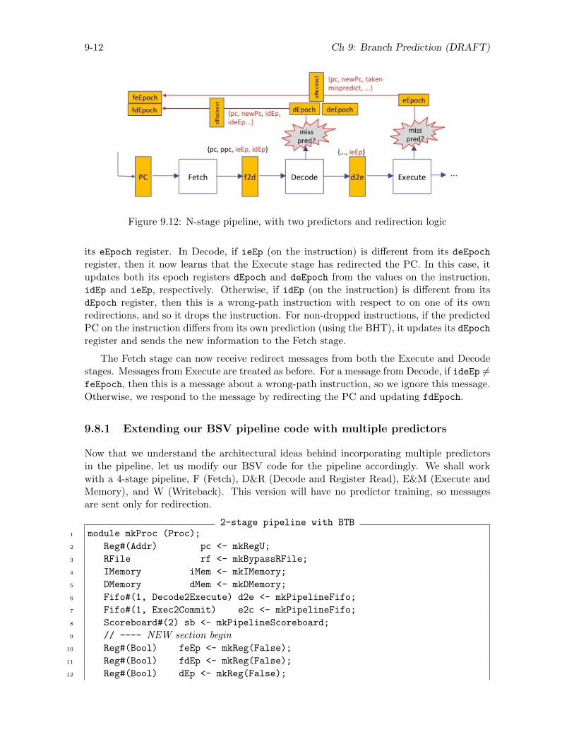
9-12 Ch 9: Branch Prediction (DRAFT)
Figure 9.12: N-stage pipeline, with two predictors and redirection logic
its eEpoch register. In Decode, if ieEp (on the instruction) is different from its deEpoch
register, then it now learns that the Execute stage has redirected the PC. In this case, itupdates both its epoch registers dEpoch and deEpoch from the values on the instruction,idEp and ieEp, respectively. Otherwise, if idEp (on the instruction) is different from itsdEpoch register, then this is a wrong-path instruction with respect to on one of its ownredirections, and so it drops the instruction. For non-dropped instructions, if the predictedPC on the instruction differs from its own prediction (using the BHT), it updates its dEpochregister and sends the new information to the Fetch stage.
The Fetch stage can now receive redirect messages from both the Execute and Decodestages. Messages from Execute are treated as before. For a message from Decode, if ideEp 6=feEpoch, then this is a message about a wrong-path instruction, so we ignore this message.Otherwise, we respond to the message by redirecting the PC and updating fdEpoch.
9.8.1 Extending our BSV pipeline code with multiple predictors
Now that we understand the architectural ideas behind incorporating multiple predictorsin the pipeline, let us modify our BSV code for the pipeline accordingly. We shall workwith a 4-stage pipeline, F (Fetch), D&R (Decode and Register Read), E&M (Execute andMemory), and W (Writeback). This version will have no predictor training, so messagesare sent only for redirection.
2-stage pipeline with BTB1 module mkProc (Proc);
2 Reg#(Addr) pc <- mkRegU;
3 RFile rf <- mkBypassRFile;
4 IMemory iMem <- mkIMemory;
5 DMemory dMem <- mkDMemory;
6 Fifo#(1, Decode2Execute) d2e <- mkPipelineFifo;
7 Fifo#(1, Exec2Commit) e2c <- mkPipelineFifo;
8 Scoreboard#(2) sb <- mkPipelineScoreboard;
9 // ---- NEW section begin10 Reg#(Bool) feEp <- mkReg(False);
11 Reg#(Bool) fdEp <- mkReg(False);
12 Reg#(Bool) dEp <- mkReg(False);
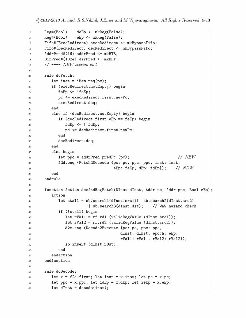
c©2012-2013 Arvind, R.S.Nikhil, J.Emer and M.Vijayaraghavan; All Rights Reserved 9-13
13 Reg#(Bool) deEp <- mkReg(False);
14 Reg#(Bool) eEp <- mkReg(False);
15 Fifo#(ExecRedirect) execRedirect <- mkBypassFifo;
16 Fifo#(DecRedirect) decRedirect <- mkBypassFifo;
17 AddrPred#(16) addrPred <- mkBTB;
18 DirPred#(1024) dirPred <- mkBHT;
19 // ---- NEW section end20
21 rule doFetch;
22 let inst = iMem.req(pc);
23 if (execRedirect.notEmpty) begin
24 feEp <= !feEp;
25 pc <= execRedirect.first.newPc;
26 execRedirect.deq;
27 end
28 else if (decRedirect.notEmpty) begin
29 if (decRedirect.first.eEp == feEp) begin
30 fdEp <= ! fdEp;
31 pc <= decRedirect.first.newPc;
32 end
33 decRedirect.deq;
34 end
35 else begin
36 let ppc = addrPred.predPc (pc); // NEW37 f2d.enq (Fetch2Decoode {pc: pc, ppc: ppc, inst: inst,
38 eEp: feEp, dEp: fdEp}); // NEW39 end
40 endrule
41
42 function Action decAndRegFetch(DInst dInst, Addr pc, Addr ppc, Bool eEp);
43 action
44 let stall = sb.search1(dInst.src1)|| sb.search2(dInst.src2)
45 || sb.search3(dInst.dst); // WAW hazard check
46 if (!stall) begin
47 let rVal1 = rf.rd1 (validRegValue (dInst.src1));
48 let rVal2 = rf.rd2 (validRegValue (dInst.src2));
49 d2e.enq (Decode2Execute {pc: pc, ppc: ppc,
50 dInst: dInst, epoch: eEp,
51 rVal1: rVal1, rVal2: rVal2});
52 sb.insert (dInst.rDst);
53 end
54 endaction
55 endfunction
56
57 rule doDecode;
58 let x = f2d.first; let inst = x.inst; let pc = x.pc;
59 let ppc = x.ppc; let idEp = x.dEp; let ieEp = x.eEp;
60 let dInst = decode(inst);
9-14 Ch 9: Branch Prediction (DRAFT)
61 let newPc = dirPrec.predAddr(pc, dInst);
62 if (ieEp != deEp) begin // change Decode’s epochs and
63 // continue normal instruction execution
64 deEp <= ieEp; let newdEp = idEp;
65 decAndRegRead (inst, pc, newPc, ieEp);
66 if (ppc != newPc) begin
67 newDEp = !newdEp;
68 decRedirect.enq (DecRedirect {pc: pc,
69 newPc: newPc, eEp: ieEp});
70 end
71 dEp <= newdEp
72 end
73 else if (idEp == dEp) begin
74 decAndRegRead (inst, pc, newPc, ieEp);
75 if (ppc != newPc) begin
76 dEp <= !dEp;
77 decRedirect.enq (DecRedirect {pc: pc,
78 newPc: newPc, eEp: ieEp});
79 end
80 end
81 f2d.deq;
82 endrule
83
84 rule doExecute;
85 let x = d2e.first;
86 let dInst = x.dInst; let pc = x.pc;
87 let ppc = x.ppc; let epoch = x.epoch;
88 let rVal1 = x.rVal1; let rVal2 = x.rVal2;
89 if (epoch == eEpoch) begin
90 let eInst = exec (dInst, rVal1, rVal2, pc, ppc);
91 if (eInst.iType == Ld)
92 eInst.data <- dMem.req (MemReq {op:Ld, addr:eInst.addr, data:?});
93 else if (eInst.iType == St)
94 let d <- dMem.req (MemReq {op:St, addr:eInst.addr, data:eInst.data});
95 e2c.enq (Exec2Commit {dst:eInst.dst, data:eInst.data});
96 if (eInst.mispredict) begin
97 execRedirect.enq (eInst.addr);
98 eEpoch <= !eEpoch;
99 end
100 end
101 else
102 e2c.enq (Exec2Commit {dst:Invalid, data:?});
103 d2e.deq;
104 endrule
105
106 rule doCommit;
107 let dst = eInst.first.dst;
108 let data = eInst.first.data;
c©2012-2013 Arvind, R.S.Nikhil, J.Emer and M.Vijayaraghavan; All Rights Reserved 9-15
109 if (isValid (dst))
110 rf.wr (validValue(dst), data);
111 e2c.deq;
112 sb.remove;
113 endrule
Lines 10-19 instantiate all the new modules and state needed for the predictors. Line38, in the Fetch rule, attaches two epoch values to each instruction sent downstream. Lines62-80 in the Decode rule perform the decode-stage prediction that we just described. Theyuse the function shown on lines 42-55. The Execute and Commit rules are completelyunchanged from before.
9.9 Conclusion
This chapter has again shown the value of thinking about processor pipelines as distributedsystems (logically independent units communicating with messages) instead of as a globallysynchronous state machine. Trying to manage the complex concurrency issues around mul-tiple branch predictors by thinking about the pipeline as a globally synchronous machinecan be very, very difficult and error-prone. The concept of epochs, distributed approxima-tions of the epoch, and messages whose exact latency does not affect correctness, allow usto design a solution that is clean and modular, and whose correctness is easier to reasonabout.

9-16 Ch 9: Branch Prediction (DRAFT)
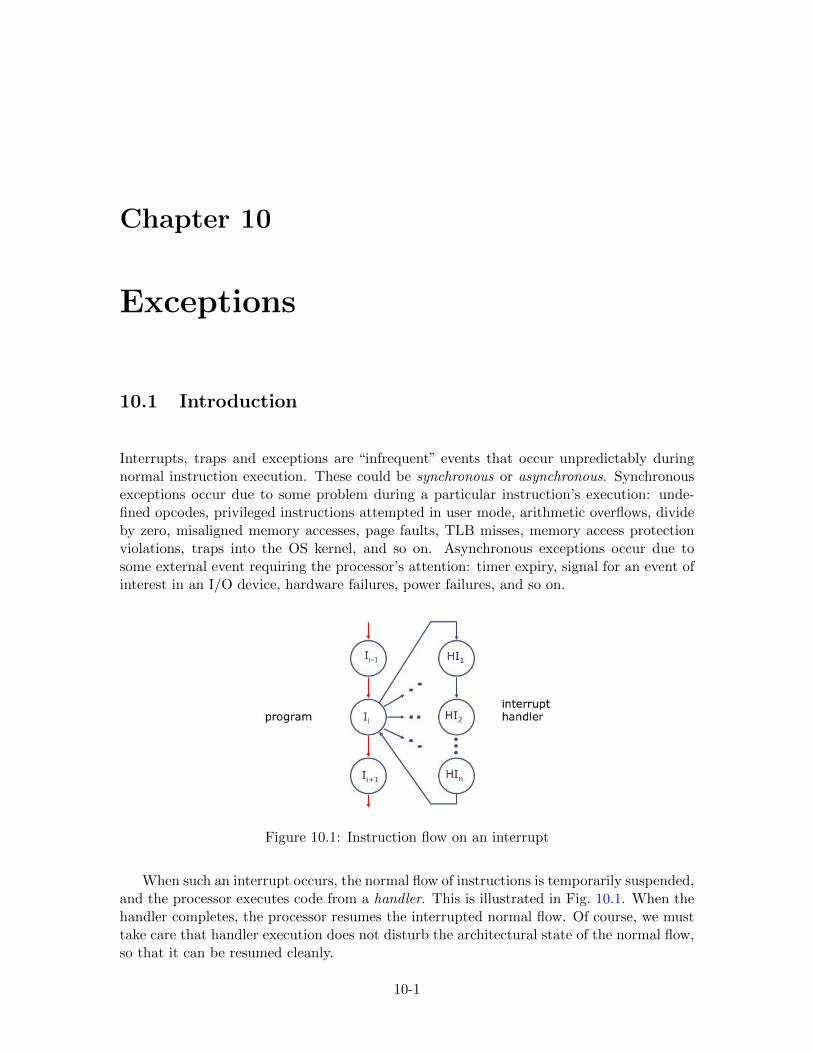
Chapter 10
Exceptions
10.1 Introduction
Interrupts, traps and exceptions are “infrequent” events that occur unpredictably duringnormal instruction execution. These could be synchronous or asynchronous. Synchronousexceptions occur due to some problem during a particular instruction’s execution: unde-fined opcodes, privileged instructions attempted in user mode, arithmetic overflows, divideby zero, misaligned memory accesses, page faults, TLB misses, memory access protectionviolations, traps into the OS kernel, and so on. Asynchronous exceptions occur due tosome external event requiring the processor’s attention: timer expiry, signal for an event ofinterest in an I/O device, hardware failures, power failures, and so on.
Figure 10.1: Instruction flow on an interrupt
When such an interrupt occurs, the normal flow of instructions is temporarily suspended,and the processor executes code from a handler. This is illustrated in Fig. 10.1. When thehandler completes, the processor resumes the interrupted normal flow. Of course, we musttake care that handler execution does not disturb the architectural state of the normal flow,so that it can be resumed cleanly.
10-1
10-2 Ch 10: Exceptions (DRAFT)
10.2 Asynchronous Interrupts
An asynchronous interrupt is typically initiated by an external device (such as a timer orI/O device) by asserting one of the prioritized interrupt request lines (IRQs) to get theprocessor’s attention. The processor may not respond immediately, since it may be in themiddle of a critical task (perhaps even in the middle of responding to a previous interrupt).
Most ISAs have a concept of precise interrupts, i.e., even though the processor mayhave a deep pipeline with many instructions simultaneously in flight, even though it maybe executing instructions in superscalar mode or out of order, there is always a well-definednotion of the interrupt occurring precisely between two instructions Ij−1 and Ij such that itis as if Ij−1 has completed and updated its architectural state, and Ij has not even started.
When the interrupt occurs, the processor saves the PC of instruction Ij in a specialregister, epc. It disables further interrupts, and jumps to a designated interrupt handlerand starts running in kernel mode. Disabling is typically done by writing to an interruptmask register which has a bit corresponding to each kind of interrupt or each externalinterrupt line; when a bit here is 0, the processor ignores interrupts from that source.Kernel mode (also sometimes called supervisor mode or privileged mode) is a special modeallowing the processor full access to all resources on the machine; this is in contrast to usermode, which is the mode in which normal application code is executed, where such accessesare prohibited (by trapping if they are attempted). Most ISAs have this kernel/user modedistinction for protection purposes, i.e., it prevents ordinary application programs fromaccessing or damaging system devices or other application programs that may be timemultiplexed concurrently by the operating sytem.
At the speeds at which modern processors operate, interrupts are a major disruption topipelined execution, and so raw speed of interrupt handling is typically not of paramountconcern.
10.2.1 Interrupt Handlers
In effect, the processor is redirected to a handler when an interrupt occurs. What is the PCtarget for this redirection? In some machines it is a known address fixed by the ISA. Othermachines have an interrupt vector at a known address, which is an array of redirection PCs.When an interrupt occurs, the kind and source of the interrupt indicate an index into thisarray, from which the processor picks up the redirection PC.
Once the PC has been redirected and the handler starts executing, it saves the epc
(the PC of the instruction to resume on handler completion). For this, the ISA has aninstruction to move the epc into a general purpose register. At least this much work mustbe done before the handler re-enables interrupts in order to handle nested interrupts. TheISA typically also has a status register that indicates the cause or source of the interrupt,so that the handler can respond accordingly.
On handler completion, it executes a special indirect jump instruction ERET (returnfrom exception) which:
• enables interrupts,• restores the processor to user mode from kernel mode, and

c©2012-2013 Arvind, R.S.Nikhil, J.Emer and M.Vijayaraghavan; All Rights Reserved 10-3
• restores the hardware status and control state so that instruction resumes where it leftoff at the interrupted instruction.
10.3 Synchronous Interrupts
A synchronous interrupt is caused by a particular instruction, and behaves like a controlhazard, i.e., the PC has to be redirected and instructions that follow in the normal flowthat are already in the pipeline have to be dropped, just like wrong-path instructions aftera misprediction. As mentioned before, the ISA defines has a special register epc in whichthe processor stores PC+4 of the interrupted instruction, and a special ERET instructionto return to normal operation after an exception handler.
Synchronous interrupts come in two flavors:
• Exceptions: The instruction cannot be completed (e.g., due to a page fault) and needsto be restarted after the exception has been handled.
• Faults or Traps: These are like system calls, i.e., deliberate calls into kernel moderoutines, and the instruction is regarded as completed.
10.3.1 Using synchronous exceptions to handle complex and infrequentinstructions
Synchronous exceptions offer an alternative implementation for complex or infrequent in-structions. For example, some processors do not implement floating point operations inhardware, because of their complexity in hardware. In such an implementation, an instruc-tion like:
mult ra, rb
causes an exception, and the handler implements a floating point multiplication algorithm insoftware. When the instruction is encountered, PC+4 is stored in epc, the handler performsthe multiplication and returns using ERET, and execution continues at PC+4 as usual.
10.3.2 Incorporating exception handling into our single-cycle processor
We need to extend many of our interfaces to express exception-related information wherevernecessary, in addition to the normal information. For example, a memory request will nowreturn a 2-tuple, {memory response, memory exception}. Our instruction definitions areextended for instructions like eret and mult, and so on.
New instructions for exceptions1 typedef enum {Unsupported, Alu, Ld, St, J, Jr, Br, Mult, ERet }
2 IType
3 deriving (Bits, Eq);
Decode has to be extended to handle the new opcodes:
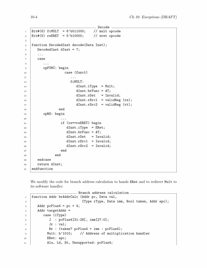
10-4 Ch 10: Exceptions (DRAFT)
Decode1 Bit#(6) fcMULT = 6’b011000; // mult opcode
2 Bit#(5) rsERET = 5’b10000; // eret opcode
3
4 function DecodedInst decode(Data Inst);
5 DecodedInst dInst = ?;
6 ...
7 case
8 ...
9 opFUNC: begin
10 case (funct)
11 ...
12 fcMULT:
13 dInst.iType = Mult;
14 dInst.brFunc = AT;
15 dInst.rDst = Invalid;
16 dInst.rSrc1 = validReg (rs);
17 dInst.rSrc2 = validReg (rt);
18 end
19 opRS: begin
20 ...
21 if (rs==rsERET) begin
22 dInst.iType = ERet;
23 dInst.brFunc = AT;
24 dInst.rDst = Invalid;
25 dInst.rSrc1 = Invalid;
26 dInst.rSrc2 = Invalid;
27 end
28 end
29 endcase
30 return dInst;
31 endfunction
We modify the code for branch address calculation to hande ERet and to redirect Mult toits software handler:
Branch address calculation1 function Addr brAddrCalc (Addr pc, Data val,
2 IType iType, Data imm, Bool taken, Addr epc);
3 Addr pcPlus4 = pc + 4;
4 Addr targetAddr =
5 case (iType)
6 J : pcPlus4[31:28], imm[27:0];
7 Jr : val;
8 Br : (taken? pcPlus4 + imm : pcPlus4);
9 Mult: h’1010; // Address of multiplication handler
10 ERet: epc;
11 Alu, Ld, St, Unsupported: pcPlus4;
c©2012-2013 Arvind, R.S.Nikhil, J.Emer and M.Vijayaraghavan; All Rights Reserved 10-5
12 endcase;
13 return targetAddr;
14 endfunction
In the code for instruction execution, we pass epc as an additional argument to the branchaddress calculator:
Instruction execution1 function ExecInst exec (DecodedInst dInst, Data rVal1,
2 Data rVal2, Addr pc, Addr epc);
3 ...
4 let brAddr = brAddrCalc (pc, rVal1, dInst.iType,
5 validValue(dInst.imm), brTaken, epc ); ...
6 eInst.brAddr = ... brAddr ...;
7 ...
8 return eInst;
9 endfunction
In the Execute rule, we load epc if it is mult instruction:
Execute rule1 rule doExecute;
2 let inst = iMem.req (pc);
3 let dInst = decode (inst);
4 let rVal1 = rf.rd1 (validRegValue (dInst.src1));
5 let rVal2 = rf.rd2 (validRegValue (dInst.src2));
6 let eInst = exec (dInst, rVal1, rVal2, pc, epc);
7 if (eInst.iType == Ld)
8 eInst.data <- dMem.req (MemReq {op: Ld, addr:
9 eInst.addr, data: ?});
10 else if (eInst.iType == St)
11 let d <- dMem.req (MemReq {op: St, addr:
12 eInst.addr, data: eInst.data});
13 if (isValid (eInst.dst))
14 rf.wr (validRegValue (eInst.dst), eInst.data);
15 pc <= eInst.brTaken ? eInst.addr : pc + 4;
16 if (eInst.iType == Mult) epc <= eInst.addr;
17 endrule
With these changes, our single-cycle implementation handles exceptions.
10.4 Incorporating exception handling into our pipelined pro-cessor
Fig. 10.2 shows that synchronous exceptions can be raised at various points in the pipeline.In Fetch, the PC address may be invalid or we may encounter a page fault. In Decode, the
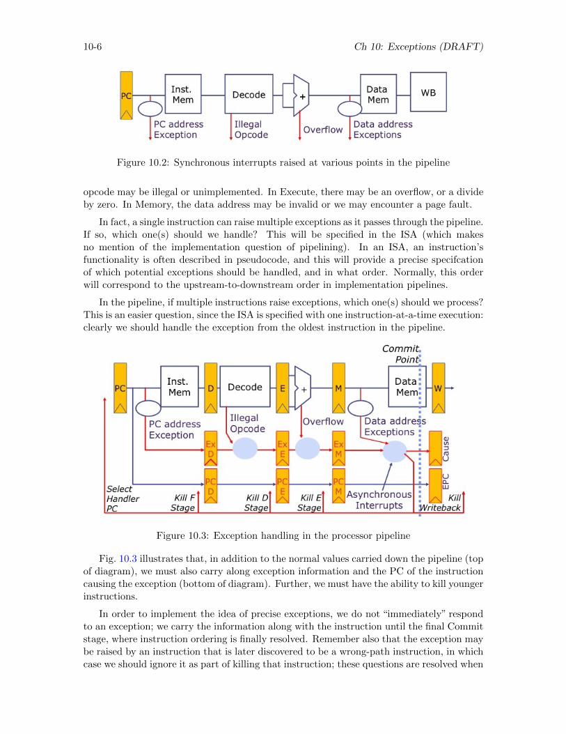
10-6 Ch 10: Exceptions (DRAFT)
Figure 10.2: Synchronous interrupts raised at various points in the pipeline
opcode may be illegal or unimplemented. In Execute, there may be an overflow, or a divideby zero. In Memory, the data address may be invalid or we may encounter a page fault.
In fact, a single instruction can raise multiple exceptions as it passes through the pipeline.If so, which one(s) should we handle? This will be specified in the ISA (which makesno mention of the implementation question of pipelining). In an ISA, an instruction’sfunctionality is often described in pseudocode, and this will provide a precise specifcationof which potential exceptions should be handled, and in what order. Normally, this orderwill correspond to the upstream-to-downstream order in implementation pipelines.
In the pipeline, if multiple instructions raise exceptions, which one(s) should we process?This is an easier question, since the ISA is specified with one instruction-at-a-time execution:clearly we should handle the exception from the oldest instruction in the pipeline.
Figure 10.3: Exception handling in the processor pipeline
Fig. 10.3 illustrates that, in addition to the normal values carried down the pipeline (topof diagram), we must also carry along exception information and the PC of the instructioncausing the exception (bottom of diagram). Further, we must have the ability to kill youngerinstructions.
In order to implement the idea of precise exceptions, we do not “immediately” respondto an exception; we carry the information along with the instruction until the final Commitstage, where instruction ordering is finally resolved. Remember also that the exception maybe raised by an instruction that is later discovered to be a wrong-path instruction, in whichcase we should ignore it as part of killing that instruction; these questions are resolved when
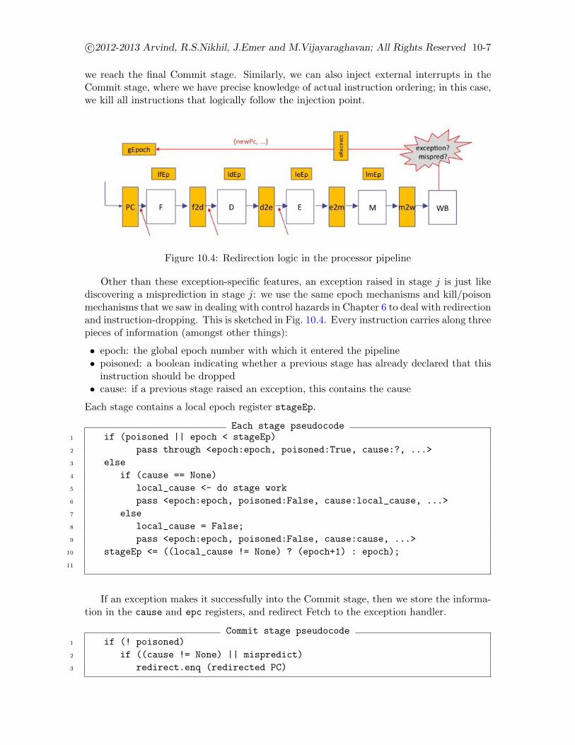
c©2012-2013 Arvind, R.S.Nikhil, J.Emer and M.Vijayaraghavan; All Rights Reserved 10-7
we reach the final Commit stage. Similarly, we can also inject external interrupts in theCommit stage, where we have precise knowledge of actual instruction ordering; in this case,we kill all instructions that logically follow the injection point.
Figure 10.4: Redirection logic in the processor pipeline
Other than these exception-specific features, an exception raised in stage j is just likediscovering a misprediction in stage j: we use the same epoch mechanisms and kill/poisonmechanisms that we saw in dealing with control hazards in Chapter 6 to deal with redirectionand instruction-dropping. This is sketched in Fig. 10.4. Every instruction carries along threepieces of information (amongst other things):
• epoch: the global epoch number with which it entered the pipeline• poisoned: a boolean indicating whether a previous stage has already declared that this
instruction should be dropped• cause: if a previous stage raised an exception, this contains the cause
Each stage contains a local epoch register stageEp.
Each stage pseudocode1 if (poisoned || epoch < stageEp)
2 pass through <epoch:epoch, poisoned:True, cause:?, ...>
3 else
4 if (cause == None)
5 local_cause <- do stage work
6 pass <epoch:epoch, poisoned:False, cause:local_cause, ...>
7 else
8 local_cause = False;
9 pass <epoch:epoch, poisoned:False, cause:cause, ...>
10 stageEp <= ((local_cause != None) ? (epoch+1) : epoch);
11
If an exception makes it successfully into the Commit stage, then we store the informa-tion in the cause and epc registers, and redirect Fetch to the exception handler.
Commit stage pseudocode1 if (! poisoned)
2 if ((cause != None) || mispredict)
3 redirect.enq (redirected PC)
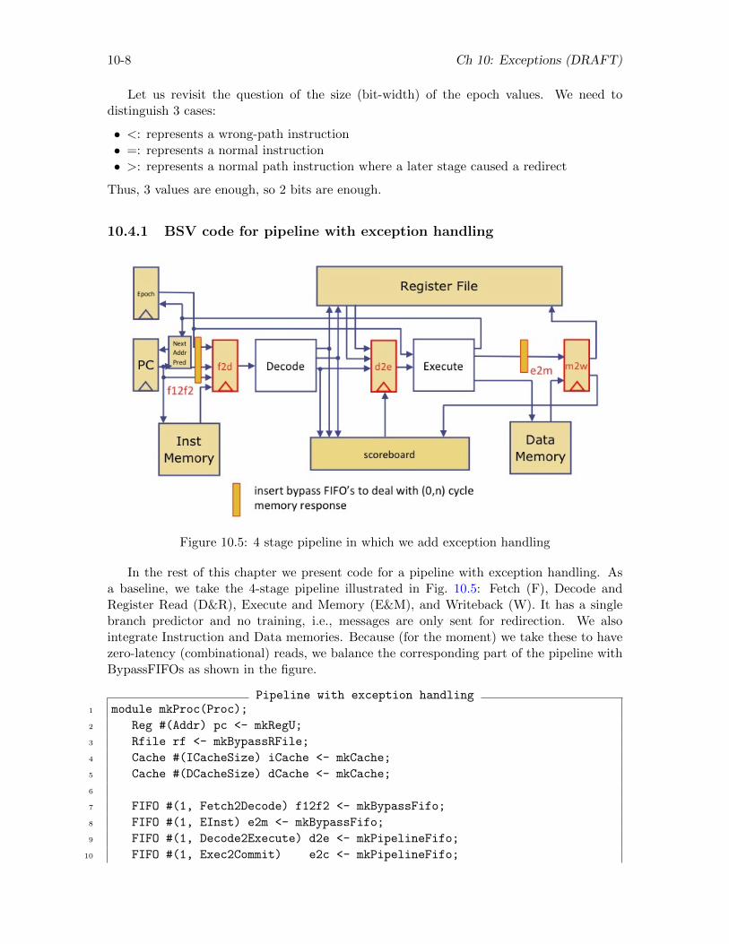
10-8 Ch 10: Exceptions (DRAFT)
Let us revisit the question of the size (bit-width) of the epoch values. We need todistinguish 3 cases:
• <: represents a wrong-path instruction• =: represents a normal instruction• >: represents a normal path instruction where a later stage caused a redirect
Thus, 3 values are enough, so 2 bits are enough.
10.4.1 BSV code for pipeline with exception handling
Figure 10.5: 4 stage pipeline in which we add exception handling
In the rest of this chapter we present code for a pipeline with exception handling. Asa baseline, we take the 4-stage pipeline illustrated in Fig. 10.5: Fetch (F), Decode andRegister Read (D&R), Execute and Memory (E&M), and Writeback (W). It has a singlebranch predictor and no training, i.e., messages are only sent for redirection. We alsointegrate Instruction and Data memories. Because (for the moment) we take these to havezero-latency (combinational) reads, we balance the corresponding part of the pipeline withBypassFIFOs as shown in the figure.
Pipeline with exception handling1 module mkProc(Proc);
2 Reg #(Addr) pc <- mkRegU;
3 Rfile rf <- mkBypassRFile;
4 Cache #(ICacheSize) iCache <- mkCache;
5 Cache #(DCacheSize) dCache <- mkCache;
6
7 FIFO #(1, Fetch2Decode) f12f2 <- mkBypassFifo;
8 FIFO #(1, EInst) e2m <- mkBypassFifo;
9 FIFO #(1, Decode2Execute) d2e <- mkPipelineFifo;
10 FIFO #(1, Exec2Commit) e2c <- mkPipelineFifo;
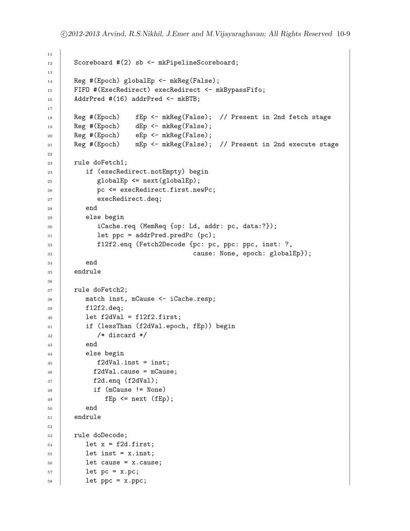
c©2012-2013 Arvind, R.S.Nikhil, J.Emer and M.Vijayaraghavan; All Rights Reserved 10-9
11
12 Scoreboard #(2) sb <- mkPipelineScoreboard;
13
14 Reg #(Epoch) globalEp <- mkReg(False);
15 FIFO #(ExecRedirect) execRedirect <- mkBypassFifo;
16 AddrPred #(16) addrPred <- mkBTB;
17
18 Reg #(Epoch) fEp <- mkReg(False); // Present in 2nd fetch stage
19 Reg #(Epoch) dEp <- mkReg(False);
20 Reg #(Epoch) eEp <- mkReg(False);
21 Reg #(Epoch) mEp <- mkReg(False); // Present in 2nd execute stage
22
23 rule doFetch1;
24 if (execRedirect.notEmpty) begin
25 globalEp <= next(globalEp);
26 pc <= execRedirect.first.newPc;
27 execRedirect.deq;
28 end
29 else begin
30 iCache.req (MemReq {op: Ld, addr: pc, data:?});
31 let ppc = addrPred.predPc (pc);
32 f12f2.enq (Fetch2Decode {pc: pc, ppc: ppc, inst: ?,
33 cause: None, epoch: globalEp});
34 end
35 endrule
36
37 rule doFetch2;
38 match inst, mCause <- iCache.resp;
39 f12f2.deq;
40 let f2dVal = f12f2.first;
41 if (lessThan (f2dVal.epoch, fEp)) begin
42 /* discard */
43 end
44 else begin
45 f2dVal.inst = inst;
46 f2dVal.cause = mCause;
47 f2d.enq (f2dVal);
48 if (mCause != None)
49 fEp <= next (fEp);
50 end
51 endrule
52
53 rule doDecode;
54 let x = f2d.first;
55 let inst = x.inst;
56 let cause = x.cause;
57 let pc = x.pc;
58 let ppc = x.ppc;
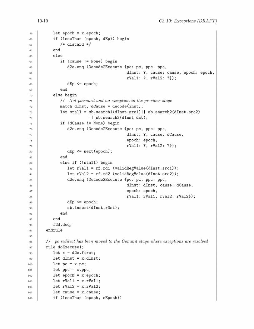
10-10 Ch 10: Exceptions (DRAFT)
59 let epoch = x.epoch;
60 if (lessThan (epoch, dEp)) begin
61 /* discard */
62 end
63 else
64 if (cause != None) begin
65 d2e.enq (Decode2Execute {pc: pc, ppc: ppc,
66 dInst: ?, cause: cause, epoch: epoch,
67 rVal1: ?, rVal2: ?});
68 dEp <= epoch;
69 end
70 else begin
71 // Not poisoned and no exception in the previous stage72 match dInst, dCause = decode(inst);
73 let stall = sb.search1(dInst.src1)|| sb.search2(dInst.src2)
74 || sb.search3(dInst.dst);
75 if (dCause != None) begin
76 d2e.enq (Decode2Execute {pc: pc, ppc: ppc,
77 dInst: ?, cause: dCause,
78 epoch: epoch,
79 rVal1: ?, rVal2: ?});
80 dEp <= next(epoch);
81 end
82 else if (!stall) begin
83 let rVal1 = rf.rd1 (validRegValue(dInst.src1));
84 let rVal2 = rf.rd2 (validRegValue(dInst.src2));
85 d2e.enq (Decode2Execute {pc: pc, ppc: ppc,
86 dInst: dInst, cause: dCause,
87 epoch: epoch,
88 rVal1: rVal1, rVal2: rVal2});
89 dEp <= epoch;
90 sb.insert(dInst.rDst);
91 end
92 end
93 f2d.deq;
94 endrule
95
96 // pc redirect has been moved to the Commit stage where exceptions are resolved97 rule doExecute1;
98 let x = d2e.first;
99 let dInst = x.dInst;
100 let pc = x.pc;
101 let ppc = x.ppc;
102 let epoch = x.epoch;
103 let rVal1 = x.rVal1;
104 let rVal2 = x.rVal2;
105 let cause = x.cause;
106 if (lessThan (epoch, eEpoch))
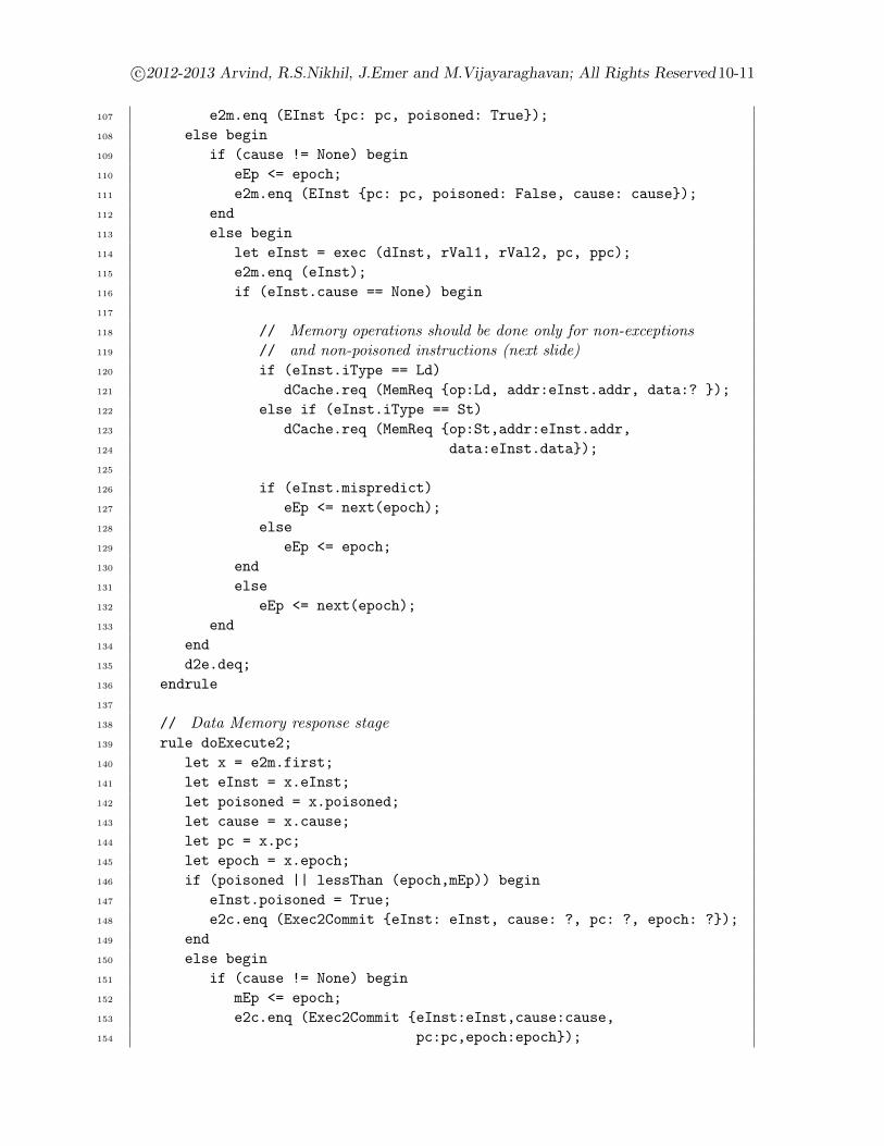
c©2012-2013 Arvind, R.S.Nikhil, J.Emer and M.Vijayaraghavan; All Rights Reserved10-11
107 e2m.enq (EInst {pc: pc, poisoned: True});
108 else begin
109 if (cause != None) begin
110 eEp <= epoch;
111 e2m.enq (EInst {pc: pc, poisoned: False, cause: cause});
112 end
113 else begin
114 let eInst = exec (dInst, rVal1, rVal2, pc, ppc);
115 e2m.enq (eInst);
116 if (eInst.cause == None) begin
117
118 // Memory operations should be done only for non-exceptions119 // and non-poisoned instructions (next slide)120 if (eInst.iType == Ld)
121 dCache.req (MemReq {op:Ld, addr:eInst.addr, data:? });
122 else if (eInst.iType == St)
123 dCache.req (MemReq {op:St,addr:eInst.addr,
124 data:eInst.data});
125
126 if (eInst.mispredict)
127 eEp <= next(epoch);
128 else
129 eEp <= epoch;
130 end
131 else
132 eEp <= next(epoch);
133 end
134 end
135 d2e.deq;
136 endrule
137
138 // Data Memory response stage139 rule doExecute2;
140 let x = e2m.first;
141 let eInst = x.eInst;
142 let poisoned = x.poisoned;
143 let cause = x.cause;
144 let pc = x.pc;
145 let epoch = x.epoch;
146 if (poisoned || lessThan (epoch,mEp)) begin
147 eInst.poisoned = True;
148 e2c.enq (Exec2Commit {eInst: eInst, cause: ?, pc: ?, epoch: ?});
149 end
150 else begin
151 if (cause != None) begin
152 mEp <= epoch;
153 e2c.enq (Exec2Commit {eInst:eInst,cause:cause,
154 pc:pc,epoch:epoch});
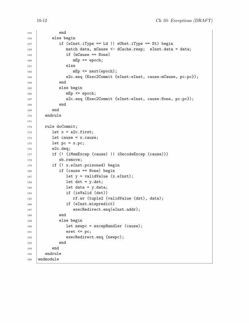
10-12 Ch 10: Exceptions (DRAFT)
155 end
156 else begin
157 if (eInst.iType == Ld || eUbst.iType == St) begin
158 match data, mCause <- dCache.resp; eInst.data = data;
159 if (mCause == None)
160 mEp <= epoch;
161 else
162 mEp <= next(epoch);
163 e2c.enq (Exec2Commit {eInst:eInst, cause:mCause, pc:pc});
164 end
165 else begin
166 mEp <= epoch;
167 e2c.enq (Exec2Commit {eInst:eInst, cause:None, pc:pc});
168 end
169 end
170 endrule
171
172 rule doCommit;
173 let x = e2c.first;
174 let cause = x.cause;
175 let pc = x.pc;
176 e2c.deq;
177 if (! (iMemExcep (cause) || iDecodeExcep (cause)))
178 sb.remove;
179 if (! x.eInst.poisoned) begin
180 if (cause == None) begin
181 let y = validValue (x.eInst);
182 let dst = y.dst;
183 let data = y.data;
184 if (isValid (dst))
185 rf.wr (tuple2 (validValue (dst), data);
186 if (eInst.mispredict)
187 execRedirect.enq(eInst.addr);
188 end
189 else begin
190 let newpc = excepHandler (cause);
191 eret <= pc;
192 execRedirect.enq (newpc);
193 end
194 end
195 endrule
196 endmodule
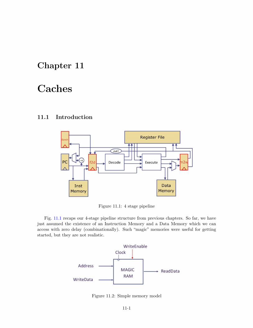
Chapter 11
Caches
11.1 Introduction
Figure 11.1: 4 stage pipeline
Fig. 11.1 recaps our 4-stage pipeline structure from previous chapters. So far, we havejust assumed the existence of an Instruction Memory and a Data Memory which we canaccess with zero delay (combinationally). Such “magic” memories were useful for gettingstarted, but they are not realistic.
Figure 11.2: Simple memory model
11-1
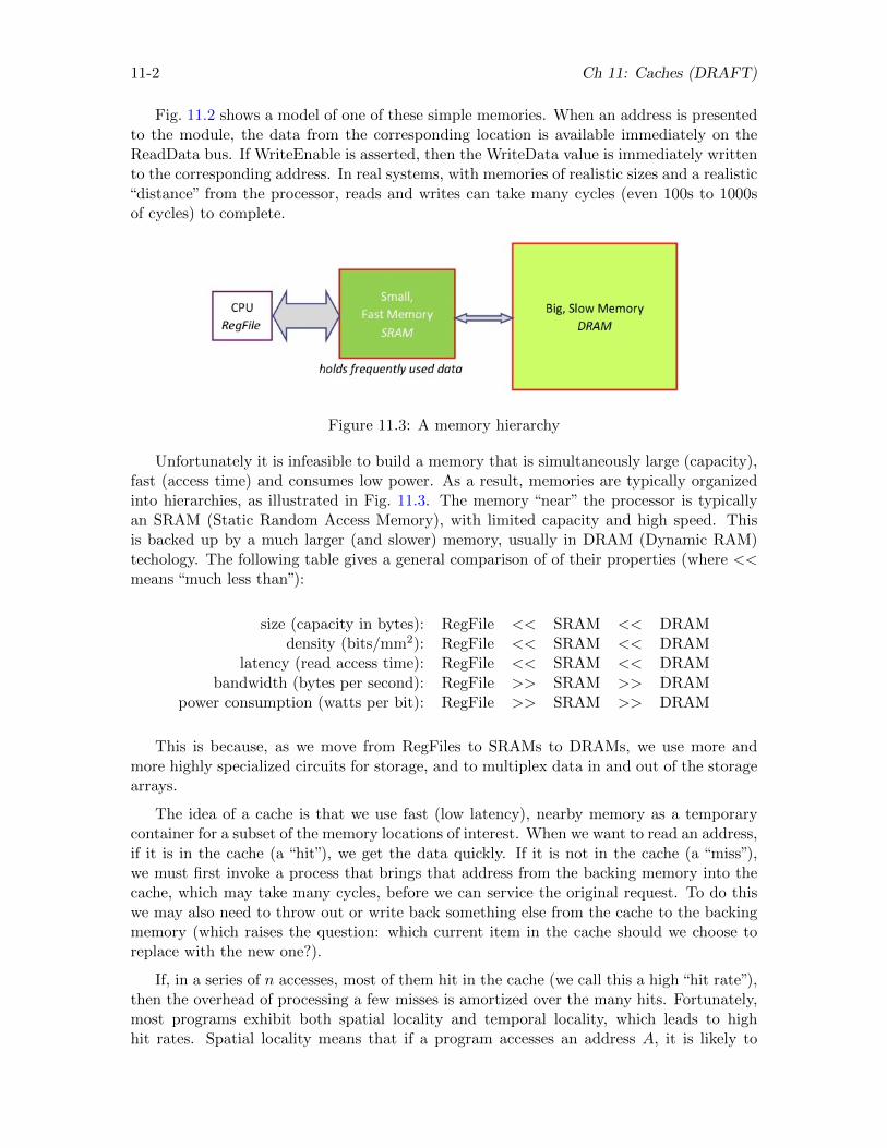
11-2 Ch 11: Caches (DRAFT)
Fig. 11.2 shows a model of one of these simple memories. When an address is presentedto the module, the data from the corresponding location is available immediately on theReadData bus. If WriteEnable is asserted, then the WriteData value is immediately writtento the corresponding address. In real systems, with memories of realistic sizes and a realistic“distance” from the processor, reads and writes can take many cycles (even 100s to 1000sof cycles) to complete.
Figure 11.3: A memory hierarchy
Unfortunately it is infeasible to build a memory that is simultaneously large (capacity),fast (access time) and consumes low power. As a result, memories are typically organizedinto hierarchies, as illustrated in Fig. 11.3. The memory “near” the processor is typicallyan SRAM (Static Random Access Memory), with limited capacity and high speed. Thisis backed up by a much larger (and slower) memory, usually in DRAM (Dynamic RAM)techology. The following table gives a general comparison of of their properties (where <<means “much less than”):
size (capacity in bytes): RegFile << SRAM << DRAMdensity (bits/mm2): RegFile << SRAM << DRAM
latency (read access time): RegFile << SRAM << DRAMbandwidth (bytes per second): RegFile >> SRAM >> DRAM
power consumption (watts per bit): RegFile >> SRAM >> DRAM
This is because, as we move from RegFiles to SRAMs to DRAMs, we use more andmore highly specialized circuits for storage, and to multiplex data in and out of the storagearrays.
The idea of a cache is that we use fast (low latency), nearby memory as a temporarycontainer for a subset of the memory locations of interest. When we want to read an address,if it is in the cache (a “hit”), we get the data quickly. If it is not in the cache (a “miss”),we must first invoke a process that brings that address from the backing memory into thecache, which may take many cycles, before we can service the original request. To do thiswe may also need to throw out or write back something else from the cache to the backingmemory (which raises the question: which current item in the cache should we choose toreplace with the new one?).
If, in a series of n accesses, most of them hit in the cache (we call this a high “hit rate”),then the overhead of processing a few misses is amortized over the many hits. Fortunately,most programs exhibit both spatial locality and temporal locality, which leads to highhit rates. Spatial locality means that if a program accesses an address A, it is likely to
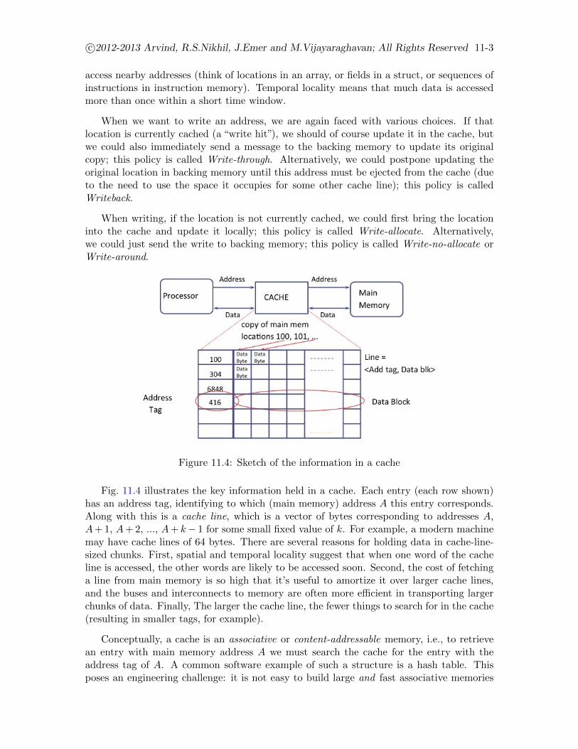
c©2012-2013 Arvind, R.S.Nikhil, J.Emer and M.Vijayaraghavan; All Rights Reserved 11-3
access nearby addresses (think of locations in an array, or fields in a struct, or sequences ofinstructions in instruction memory). Temporal locality means that much data is accessedmore than once within a short time window.
When we want to write an address, we are again faced with various choices. If thatlocation is currently cached (a “write hit”), we should of course update it in the cache, butwe could also immediately send a message to the backing memory to update its originalcopy; this policy is called Write-through. Alternatively, we could postpone updating theoriginal location in backing memory until this address must be ejected from the cache (dueto the need to use the space it occupies for some other cache line); this policy is calledWriteback.
When writing, if the location is not currently cached, we could first bring the locationinto the cache and update it locally; this policy is called Write-allocate. Alternatively,we could just send the write to backing memory; this policy is called Write-no-allocate orWrite-around.
Figure 11.4: Sketch of the information in a cache
Fig. 11.4 illustrates the key information held in a cache. Each entry (each row shown)has an address tag, identifying to which (main memory) address A this entry corresponds.Along with this is a cache line, which is a vector of bytes corresponding to addresses A,A+ 1, A+ 2, ..., A+ k− 1 for some small fixed value of k. For example, a modern machinemay have cache lines of 64 bytes. There are several reasons for holding data in cache-line-sized chunks. First, spatial and temporal locality suggest that when one word of the cacheline is accessed, the other words are likely to be accessed soon. Second, the cost of fetchinga line from main memory is so high that it’s useful to amortize it over larger cache lines,and the buses and interconnects to memory are often more efficient in transporting largerchunks of data. Finally, The larger the cache line, the fewer things to search for in the cache(resulting in smaller tags, for example).
Conceptually, a cache is an associative or content-addressable memory, i.e., to retrievean entry with main memory address A we must search the cache for the entry with theaddress tag of A. A common software example of such a structure is a hash table. Thisposes an engineering challenge: it is not easy to build large and fast associative memories
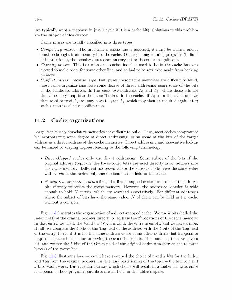
11-4 Ch 11: Caches (DRAFT)
(we typically want a response in just 1 cycle if it is a cache hit). Solutions to this problemare the subject of this chapter.
Cache misses are usually classified into three types:
• Compulsory misses: The first time a cache line is accessed, it must be a miss, and itmust be brought from memory into the cache. On large, long-running programs (billionsof instructions), the penalty due to compulsory misses becomes insignificant.• Capacity misses: This is a miss on a cache line that used to be in the cache but was
ejected to make room for some other line, and so had to be retrieved again from backingmemory.• Conflict misses: Because large, fast, purely associative memories are difficult to build,
most cache organizations have some degree of direct addressing using some of the bitsof the candidate address. In this case, two addresses A1 and A2, where those bits arethe same, may map into the same “bucket” in the cache. If A1 is in the cache and wethen want to read A2, we may have to eject A1, which may then be required again later;such a miss is called a conflict miss.
11.2 Cache organizations
Large, fast, purely associative memories are difficult to build. Thus, most caches compromiseby incorporating some degree of direct addressing, using some of the bits of the targetaddress as a direct address of the cache memories. Direct addressing and associative lookupcan be mixed to varying degrees, leading to the following terminology:
• Direct-Mapped caches only use direct addressing. Some subset of the bits of theoriginal address (typically the lower-order bits) are used directly as an address intothe cache memory. Different addresses where the subset of bits have the same valuewill collide in the cache; only one of them can be held in the cache.
• N -way Set-Associative caches first, like direct-mapped caches, use some of the addressbits directly to access the cache memory. However, the addressed location is wideenough to hold N entries, which are searched associatively. For different addresseswhere the subset of bits have the same value, N of them can be held in the cachewithout a collision.
Fig. 11.5 illustrates the organization of a direct-mapped cache. We use k bits (called theIndex field) of the original address directly to address the 2k locations of the cache memory.In that entry, we check the Valid bit (V); if invalid, the entry is empty, and we have a miss.If full, we compare the t bits of the Tag field of the address with the t bits of the Tag fieldof the entry, to see if it is for the same address or for some other address that happens tomap to the same bucket due to having the same Index bits. If it matches, then we have ahit, and we use the b bits of the Offset field of the original address to extract the relevantbyte(s) of the cache line.
Fig. 11.6 illustrates how we could have swapped the choice of t and k bits for the Indexand Tag from the original address. In fact, any partitioning of the top t+ k bits into t andk bits would work. But it is hard to say which choice will result in a higher hit rate, sinceit depends on how programs and data are laid out in the address space.
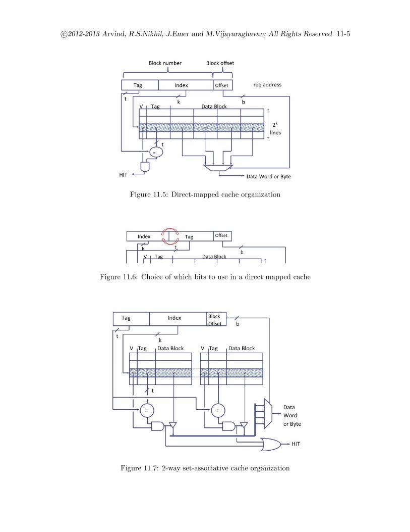
c©2012-2013 Arvind, R.S.Nikhil, J.Emer and M.Vijayaraghavan; All Rights Reserved 11-5
Figure 11.5: Direct-mapped cache organization
Figure 11.6: Choice of which bits to use in a direct mapped cache
Figure 11.7: 2-way set-associative cache organization
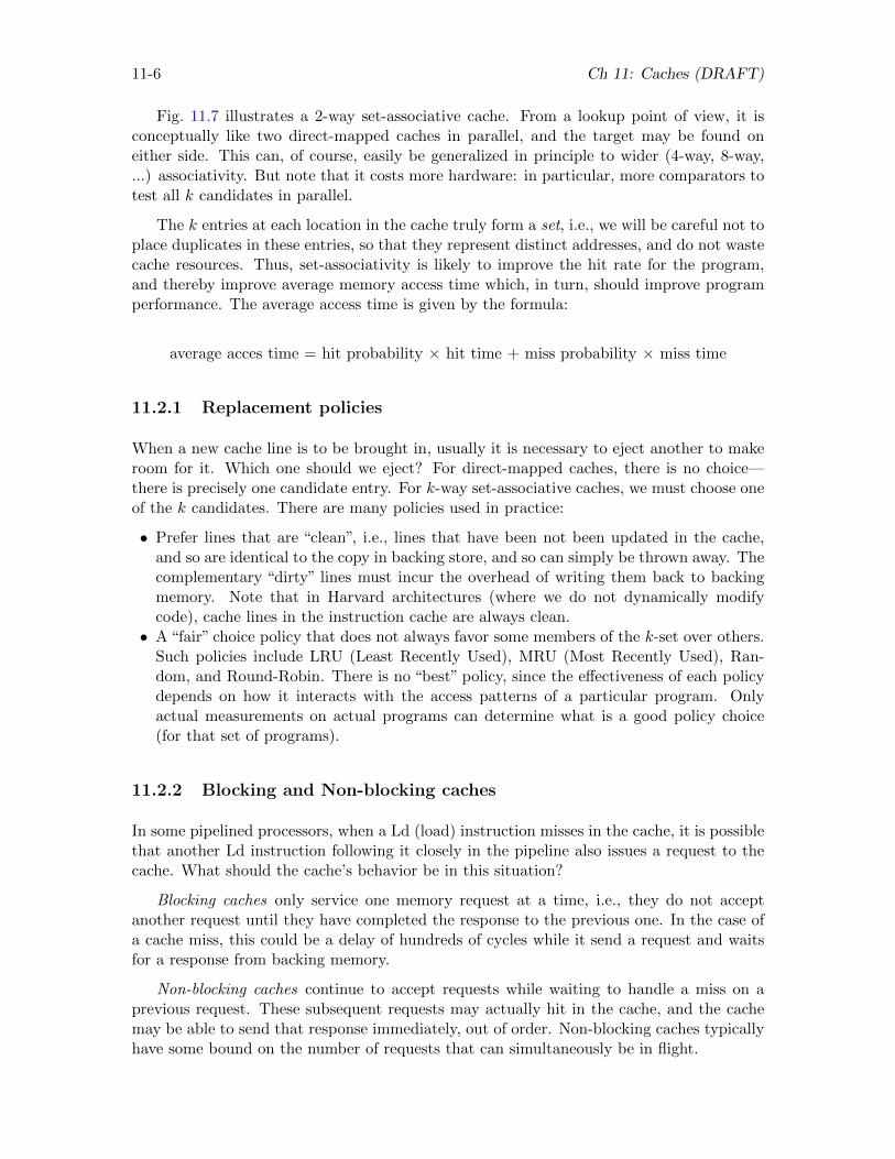
11-6 Ch 11: Caches (DRAFT)
Fig. 11.7 illustrates a 2-way set-associative cache. From a lookup point of view, it isconceptually like two direct-mapped caches in parallel, and the target may be found oneither side. This can, of course, easily be generalized in principle to wider (4-way, 8-way,...) associativity. But note that it costs more hardware: in particular, more comparators totest all k candidates in parallel.
The k entries at each location in the cache truly form a set, i.e., we will be careful not toplace duplicates in these entries, so that they represent distinct addresses, and do not wastecache resources. Thus, set-associativity is likely to improve the hit rate for the program,and thereby improve average memory access time which, in turn, should improve programperformance. The average access time is given by the formula:
average acces time = hit probability × hit time + miss probability × miss time
11.2.1 Replacement policies
When a new cache line is to be brought in, usually it is necessary to eject another to makeroom for it. Which one should we eject? For direct-mapped caches, there is no choice—there is precisely one candidate entry. For k-way set-associative caches, we must choose oneof the k candidates. There are many policies used in practice:
• Prefer lines that are “clean”, i.e., lines that have been not been updated in the cache,and so are identical to the copy in backing store, and so can simply be thrown away. Thecomplementary “dirty” lines must incur the overhead of writing them back to backingmemory. Note that in Harvard architectures (where we do not dynamically modifycode), cache lines in the instruction cache are always clean.• A “fair” choice policy that does not always favor some members of the k-set over others.
Such policies include LRU (Least Recently Used), MRU (Most Recently Used), Ran-dom, and Round-Robin. There is no “best” policy, since the effectiveness of each policydepends on how it interacts with the access patterns of a particular program. Onlyactual measurements on actual programs can determine what is a good policy choice(for that set of programs).
11.2.2 Blocking and Non-blocking caches
In some pipelined processors, when a Ld (load) instruction misses in the cache, it is possiblethat another Ld instruction following it closely in the pipeline also issues a request to thecache. What should the cache’s behavior be in this situation?
Blocking caches only service one memory request at a time, i.e., they do not acceptanother request until they have completed the response to the previous one. In the case ofa cache miss, this could be a delay of hundreds of cycles while it send a request and waitsfor a response from backing memory.
Non-blocking caches continue to accept requests while waiting to handle a miss on aprevious request. These subsequent requests may actually hit in the cache, and the cachemay be able to send that response immediately, out of order. Non-blocking caches typicallyhave some bound on the number of requests that can simultaneously be in flight.
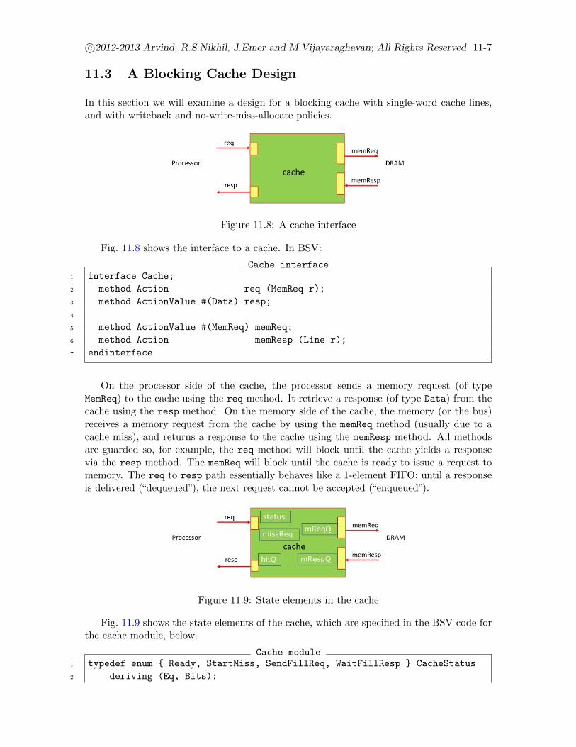
c©2012-2013 Arvind, R.S.Nikhil, J.Emer and M.Vijayaraghavan; All Rights Reserved 11-7
11.3 A Blocking Cache Design
In this section we will examine a design for a blocking cache with single-word cache lines,and with writeback and no-write-miss-allocate policies.
Figure 11.8: A cache interface
Fig. 11.8 shows the interface to a cache. In BSV:
Cache interface1 interface Cache;
2 method Action req (MemReq r);
3 method ActionValue #(Data) resp;
4
5 method ActionValue #(MemReq) memReq;
6 method Action memResp (Line r);
7 endinterface
On the processor side of the cache, the processor sends a memory request (of typeMemReq) to the cache using the req method. It retrieve a response (of type Data) from thecache using the resp method. On the memory side of the cache, the memory (or the bus)receives a memory request from the cache by using the memReq method (usually due to acache miss), and returns a response to the cache using the memResp method. All methodsare guarded so, for example, the req method will block until the cache yields a responsevia the resp method. The memReq will block until the cache is ready to issue a request tomemory. The req to resp path essentially behaves like a 1-element FIFO: until a responseis delivered (“dequeued”), the next request cannot be accepted (“enqueued”).
Figure 11.9: State elements in the cache
Fig. 11.9 shows the state elements of the cache, which are specified in the BSV code forthe cache module, below.
Cache module1 typedef enum { Ready, StartMiss, SendFillReq, WaitFillResp } CacheStatus
2 deriving (Eq, Bits);
11-8 Ch 11: Caches (DRAFT)
3
4 module mkCache (Cache);
5 // Controls cache state machine
6 Reg #(CacheStatus) status <- mkReg (Ready);
7
8 // The cache memory
9 RegFile #(CacheIndex, Line) dataArray <- mkRegFileFull;
10 RegFile #(CacheIndex, Maybe #(CacheTag)) tagArray <- mkRegFileFull;
11 RegFile #(CacheIndex, Bool) dirtyArray <- mkRegFileFull;
12
13 FIFO #(Data) hitQ <- mkBypassFIFO; // Allows 0-cycle hit responses14 Reg #(MemReq) missReq <- mkRegU;
15
16 FIFO #(MemReq) memReqQ <- mkCFFIFO;
17 FIFO #(Line) memRespQ <- mkCFFIFO;
18
19 function CacheIndex idxOf (Addr addr) = truncate (addr >> 2);
20 function CacheTag tagOf (Addr addr) = truncateLSB (addr);
21
22 rule startMiss (status == StartMiss);
23 let idx = idxOf (missReq.addr);
24 let tag = tagArray.sub (idx);
25 let dirty = dirtyArray.sub (idx);
26 if (isValid (tag) && dirty) begin // writeback
27 let addr = {validValue(tag), idx, 2’b0};
28 let data = dataArray.sub (idx);
29 memReqQ.enq (MemReq {op: St, addr: addr, data: data});
30 end
31 status <= SendFillReq;
32 endrule
33
34 rule sendFillReq (status == SendFillReq);
35 memReqQ.enq (missReq);
36 status <= WaitFillResp;
37 endrule
38
39 rule waitFillResp (status == WaitFillResp);
40 let idx = idxOf (missReq.addr);
41 let tag = tagOf (missReq.addr);
42 let data = memRespQ.first;
43 dataArray.upd (idx, data);
44 tagArray.upd (idx, tagge Valid tag);
45 dirtyArray.upd (idx, False);
46 hitQ.enq (data);
47 memRespQ.deq;
48 status <= Ready;
49 endrule
50
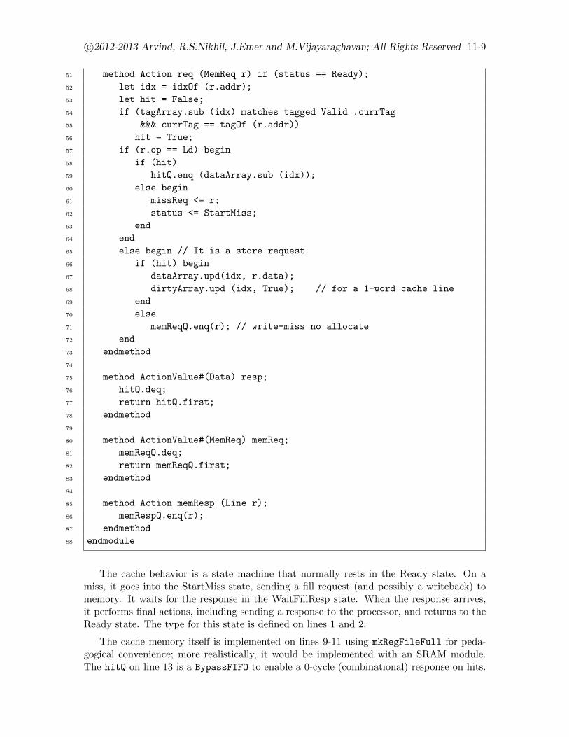
c©2012-2013 Arvind, R.S.Nikhil, J.Emer and M.Vijayaraghavan; All Rights Reserved 11-9
51 method Action req (MemReq r) if (status == Ready);
52 let idx = idxOf (r.addr);
53 let hit = False;
54 if (tagArray.sub (idx) matches tagged Valid .currTag
55 &&& currTag == tagOf (r.addr))
56 hit = True;
57 if (r.op == Ld) begin
58 if (hit)
59 hitQ.enq (dataArray.sub (idx));
60 else begin
61 missReq <= r;
62 status <= StartMiss;
63 end
64 end
65 else begin // It is a store request
66 if (hit) begin
67 dataArray.upd(idx, r.data);
68 dirtyArray.upd (idx, True); // for a 1-word cache line
69 end
70 else
71 memReqQ.enq(r); // write-miss no allocate
72 end
73 endmethod
74
75 method ActionValue#(Data) resp;
76 hitQ.deq;
77 return hitQ.first;
78 endmethod
79
80 method ActionValue#(MemReq) memReq;
81 memReqQ.deq;
82 return memReqQ.first;
83 endmethod
84
85 method Action memResp (Line r);
86 memRespQ.enq(r);
87 endmethod
88 endmodule
The cache behavior is a state machine that normally rests in the Ready state. On amiss, it goes into the StartMiss state, sending a fill request (and possibly a writeback) tomemory. It waits for the response in the WaitFillResp state. When the response arrives,it performs final actions, including sending a response to the processor, and returns to theReady state. The type for this state is defined on lines 1 and 2.
The cache memory itself is implemented on lines 9-11 using mkRegFileFull for peda-gogical convenience; more realistically, it would be implemented with an SRAM module.The hitQ on line 13 is a BypassFIFO to enable a 0-cycle (combinational) response on hits.
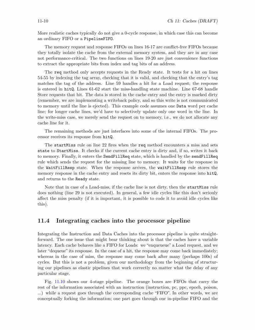
11-10 Ch 11: Caches (DRAFT)
More realistic caches typically do not give a 0-cycle response, in which case this can becomean ordinary FIFO or a PipelineFIFO.
The memory request and response FIFOs on lines 16-17 are conflict-free FIFOs becausethey totally isolate the cache from the external memory system, and they are in any casenot performance-critical. The two functions on lines 19-20 are just convenience functionsto extract the appropriate bits from index and tag bits of an address.
The req method only accepts requests in the Ready state. It tests for a hit on lines54-55 by indexing the tag array, checking that it is valid, and checking that the entry’s tagmatches the tag of the address. Line 59 handles a hit for a Load request; the responseis entered in hitQ. Lines 61-62 start the miss-handling state machine. Line 67-68 handleStore requests that hit. The data is stored in the cache entry and the entry is marked dirty(remember, we are implementing a writeback policy, and so this write is not communicatedto memory until the line is ejected). This example code assumes one Data word per cacheline; for longer cache lines, we’d have to selectively update only one word in the line. Inthe write-miss case, we merely send the request on to memory, i.e., we do not allocate anycache line for it.
The remaining methods are just interfaces into some of the internal FIFOs. The pro-cessor receives its response from hitQ.
The startMiss rule on line 22 fires when the req method encounters a miss and setsstate to StartMiss. It checks if the current cache entry is dirty and, if so, writes it backto memory. Finally, it enters the SendFillReq state, which is handled by the sendFillReq
rule which sends the request for the missing line to memory. It waits for the response inthe WaitFillResp state. When the response arrives, the waitFillResp rule stores thememory response in the cache entry and resets its dirty bit, enters the response into hitQ,and returns to the Ready state.
Note that in case of a Load-miss, if the cache line is not dirty, then the startMiss ruledoes nothing (line 29 is not executed). In general, a few idle cycles like this don’t serioulyaffect the miss penalty (if it is important, it is possible to code it to avoid idle cycles likethis).
11.4 Integrating caches into the processor pipeline
Integrating the Instruction and Data Caches into the processor pipeline is quite straight-forward. The one issue that might bear thinking about is that the caches have a variablelatency. Each cache behaves like a FIFO for Loads: we “enqueueue” a Load request, and welater “dequeue” its response. In the case of a hit, the response may come back immediately;whereas in the case of miss, the response may come back after many (perhaps 100s) ofcycles. But this is not a problem, given our methodology from the beginning of structur-ing our pipelines as elastic pipelines that work correctly no matter what the delay of anyparticular stage.
Fig. 11.10 shows our 4-stage pipeline. The orange boxes are FIFOs that carry therest of the information associated with an instruction (instruction, pc, ppc, epoch, poison,...) while a request goes through the corresponding cache “FIFO”. In other words, we areconceptually forking the information; one part goes through our in-pipeline FIFO and the
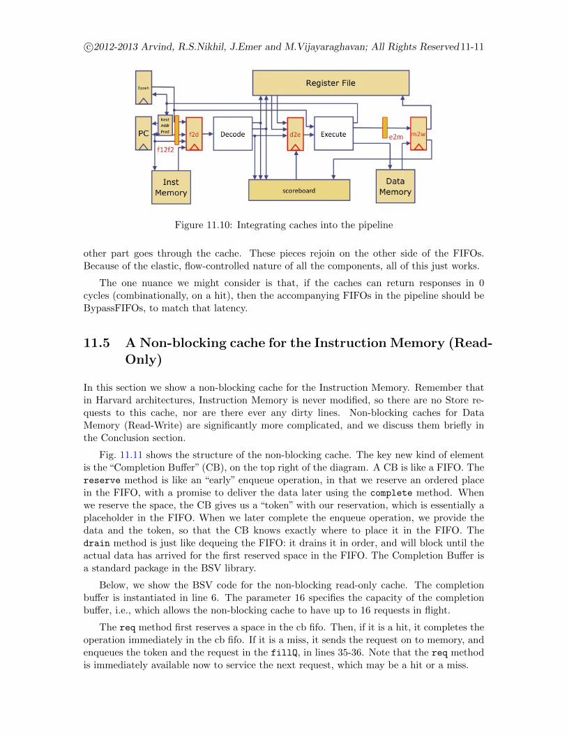
c©2012-2013 Arvind, R.S.Nikhil, J.Emer and M.Vijayaraghavan; All Rights Reserved11-11
Figure 11.10: Integrating caches into the pipeline
other part goes through the cache. These pieces rejoin on the other side of the FIFOs.Because of the elastic, flow-controlled nature of all the components, all of this just works.
The one nuance we might consider is that, if the caches can return responses in 0cycles (combinationally, on a hit), then the accompanying FIFOs in the pipeline should beBypassFIFOs, to match that latency.
11.5 A Non-blocking cache for the Instruction Memory (Read-Only)
In this section we show a non-blocking cache for the Instruction Memory. Remember thatin Harvard architectures, Instruction Memory is never modified, so there are no Store re-quests to this cache, nor are there ever any dirty lines. Non-blocking caches for DataMemory (Read-Write) are significantly more complicated, and we discuss them briefly inthe Conclusion section.
Fig. 11.11 shows the structure of the non-blocking cache. The key new kind of elementis the “Completion Buffer” (CB), on the top right of the diagram. A CB is like a FIFO. Thereserve method is like an “early” enqueue operation, in that we reserve an ordered placein the FIFO, with a promise to deliver the data later using the complete method. Whenwe reserve the space, the CB gives us a “token” with our reservation, which is essentially aplaceholder in the FIFO. When we later complete the enqueue operation, we provide thedata and the token, so that the CB knows exactly where to place it in the FIFO. Thedrain method is just like dequeing the FIFO: it drains it in order, and will block until theactual data has arrived for the first reserved space in the FIFO. The Completion Buffer isa standard package in the BSV library.
Below, we show the BSV code for the non-blocking read-only cache. The completionbuffer is instantiated in line 6. The parameter 16 specifies the capacity of the completionbuffer, i.e., which allows the non-blocking cache to have up to 16 requests in flight.
The req method first reserves a space in the cb fifo. Then, if it is a hit, it completes theoperation immediately in the cb fifo. If it is a miss, it sends the request on to memory, andenqueues the token and the request in the fillQ, in lines 35-36. Note that the req methodis immediately available now to service the next request, which may be a hit or a miss.
11-12 Ch 11: Caches (DRAFT)
Figure 11.11: Non-blocking cache for Instruction Memory
Independently, when a fill response comes back from memory, the fill rule collectsit and the information in the fillQ, updates the cache information and then invokes thecomplete method on the completion buffer. In the meanwhile, the req method could haveaccepted several more requests, some of which may be hits that are already in the completionbuffer.
The resp method returns the responses in the proper order by using the drain methodof the completion buffer.
Non-blocking Read-Only Cache module1 module mkNBCache (Cache);
2 // The cache memory
3 RegFile #(CacheIndex, Line) dataArray <- mkRegFileFull;
4 RegFile #(CacheIndex, Maybe #(CacheTag)) tagArray <- mkRegFileFull;
5
6 CompletionBuffer #(16, Data) cb <- mkCompletionBuffer;
7 FIFO #(Tuple2 #(Token, MemReq)) fillQ <- mkFIFO;
8
9 FIFO #(MemReq) memReqQ <- mkCFFIFO;
10 FIFO #(Line) memRespQ <- mkCFFIFO;
11
12 function CacheIndex idxOf (Addr addr) = truncate (addr >> 2);
13 function CacheTag tagOf (Addr addr) = truncateLSB (addr);
14
15 rule fill;
16 match .token, .req = fillQ.first; fillQ.deq;
17 data = memRespQ.first; memRespQ.deq;
18
19 let idx = idxOf (req.addr);
20 let tag = tagOf (req.addr);
c©2012-2013 Arvind, R.S.Nikhil, J.Emer and M.Vijayaraghavan; All Rights Reserved11-13
21 dataArray.upd (idx, data);
22 tagArray.upd (idx, tagged Valid tag);
23
24 cb.complete.put (tuple2 (token, dataArray.sub (idx)))
25 endrule
26
27 method Action req (MemReq r);
28 let token <- cb.reserve.get;
29 if (tagArray.sub (idxOf (r.addr)) matches tagged Valid .currTag
30 &&& currTag == tagOf (r.addr))
31 // hit
32 cb.complete.put (token, dataArray.sub (idx));
33 else begin
34 // miss
35 fillQ.enq (tuple2 (token, r));
36 memReqQ.enq (r); // send request to memory
37 end
38 endmethod
39
40 method ActionValue#(Data) resp;
41 let d <- cb.drain.get
42 return d;
43 endmethod
44
45 method ActionValue#(MemReq) memReq;
46 memReqQ.deq;
47 return memReqQ.first;
48 endmethod
49
50 method Action memResp (Line r);
51 memRespQ.enq (r);
52 endmethod
53 endmodule
How big should the fillQ be? Suppose it has size 2. Then, after the req method hashandled 2 misses by sending 2 requests to memory and enqueuing 2 items into fillQ, thenfillQ is full until the first response from memory returns and rule fill dequeues an itemfrom fillQ. Method req will then be stuck on the next miss, since it will be blocked fromenqueueing into fillQ. Thus, the capacity of fillQ is a measure of how many requeststo memory can be outstanding, i.e., still in flight without a response yet. This choice is adesign decision.
11.5.1 Completion Buffers
Here we show the code for a Completion Buffer, which is quite easy to implement usingEHRs. First, here are some type definitions for completion buffer tokens (FIFO placehold-
11-14 Ch 11: Caches (DRAFT)
ers) and the interface. The interface is parameterized by n, the desired capacity, and t, thetype of data stored in the buffer.
Completion Buffer token and interface types1 typedef struct UInt #(TLog #(n)) ix; CBToken2 #(numeric type n)
2 deriving (Bits);
3
4 interface CompletionBuffer2 #(numeric type n, type t);
5 interface Get #(CBToken2 #(n)) reserve;
6 interface Put #(Tuple2 #(CBToken2 #(n), t)) complete;
7 interface Get #(t) drain;
8 endinterface
Completion Buffer module1 module mkCompletionBuffer2 (CompletionBuffer2 #(n, t))
2 provisos (Bits #(t, tsz),
3 Log #(n, logn));
4
5 // The following FIFOs are just used to register inputs and outputs
6 // before they fan-out to/fan-in from the vr_data array
7 FIFOF #(Tuple2 #(CBToken2 #(n), t)) f_inputs <- mkFIFOF;
8 FIFOF #(t) f_outputs <- mkFIFOF;
9
10 // This is the reorder buffer
11 Vector #(n, Reg #(Maybe #(t))) vr_data <- replicateM (mkInvalidReg);
12
13 // Metadata for the reorder buffer
14 EHR #(3, Tuple3 #(UInt #(logn),
15 UInt #(logn),
16 Bool)) ehr_head_next_full
17 <- mkEHR (tuple3 (0,0, False));
18
19 match .head0, .next0, .full0 = ehr_head_next_full.ports [0];
20 match .head1, .next1, .full1 = ehr_head_next_full.ports [1];
21
22 function UInt #(logn) modulo_incr (UInt #(logn) j);
23 return ( (j == fromInteger (valueOf (n) - 1)) ? 0 : j+1);
24 endfunction
25
26 rule rl_move_inputs;
27 let t2 = f_inputs.first; f_inputs.deq;
28 match .tok, .x = t2;
29 vr_data [tok.ix] <= tagged Valid x;
30 endrule
31
32 rule rl_move_outputs (vr_data [head0] matches tagged Valid .v
33 &&& ((head0 != next0) || full0));
34 vr_data [head0] <= tagged Invalid;
35 ehr_head_next_full.ports [0] <= tuple3 (modulo_incr (head0),
c©2012-2013 Arvind, R.S.Nikhil, J.Emer and M.Vijayaraghavan; All Rights Reserved11-15
36 next0, False);
37 f_outputs.enq (v);
38 endrule
39
40 // ----------------------------------------------------------------
41 // Interface
42
43 interface Get reserve;
44 method ActionValue #(CBToken2 #(n)) get () if (! full1);
45 let next1_prime = modulo_incr (next1);
46 ehr_head_next_full.ports [1] <= tuple3 (head1,
47 next1_prime,
48 (head1==next1_prime));
49 return CBToken2 ix: next1 ;
50 endmethod
51 endinterface
52
53 interface complete = toPut (f_inputs);
54 interface drain = toGet (f_outputs);
55 endmodule
11.6 Conclusion
In the previous section, even though the non-blocking cache could accept and service mul-tiple requests, it returned responses in standard FIFO order. More sophisticated processordesigns will expose the out-of-order responses into the processor, i.e., the cache would re-turn responses immediately, and the processor may go ahead to execute those instructionsif it were safe to do so. In this case, the processor itself will associate a token with eachrequest, and the cache would return this token with the corresponding response; this allowsthe processor to know which request each response corresponds to.
Non-blocking caches for the Data Memory are more complex, because we can thenencounter RAW (Read-After-Write) hazards corresponding to memory locations, analogousto the RAW hazards we saw in Chapter 8 that concerned register file locations. For example,suppose the cache gets a read request Q1 which misses; it initiates the request to memory,and is pending the response. Suppose now it gets a write request Q2 for the same cacheline. Clearly it must wait for the pending memory read response; it must respond to theprocessor for Q1 based on the data returned from memory; and only then can it process Q2
by updating the cache line. If we allow several such interactions to be in progress acrossdifferent cache lines, the design becomes that much more complex.
In this chapter we have barely scratched the surface on the subject of caches. High-performance memory systems, which revolve around clever cache design, is one of the majorsubjects in Computer Architecture, since it is such a major determinant of program andsystem performance.

11-16 Ch 11: Caches (DRAFT)
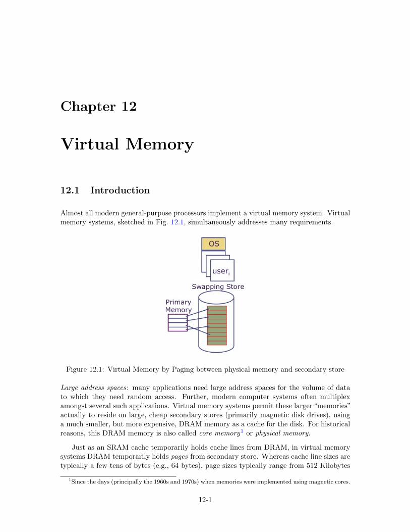
Chapter 12
Virtual Memory
12.1 Introduction
Almost all modern general-purpose processors implement a virtual memory system. Virtualmemory systems, sketched in Fig. 12.1, simultaneously addresses many requirements.
Figure 12.1: Virtual Memory by Paging between physical memory and secondary store
Large address spaces: many applications need large address spaces for the volume of datato which they need random access. Further, modern computer systems often multiplexamongst several such applications. Virtual memory systems permit these larger “memories”actually to reside on large, cheap secondary stores (primarily magnetic disk drives), usinga much smaller, but more expensive, DRAM memory as a cache for the disk. For historicalreasons, this DRAM memory is also called core memory1 or physical memory.
Just as an SRAM cache temporarily holds cache lines from DRAM, in virtual memorysystems DRAM temporarily holds pages from secondary store. Whereas cache line sizes aretypically a few tens of bytes (e.g., 64 bytes), page sizes typically range from 512 Kilobytes
1Since the days (principally the 1960s and 1970s) when memories were implemented using magnetic cores.
12-1
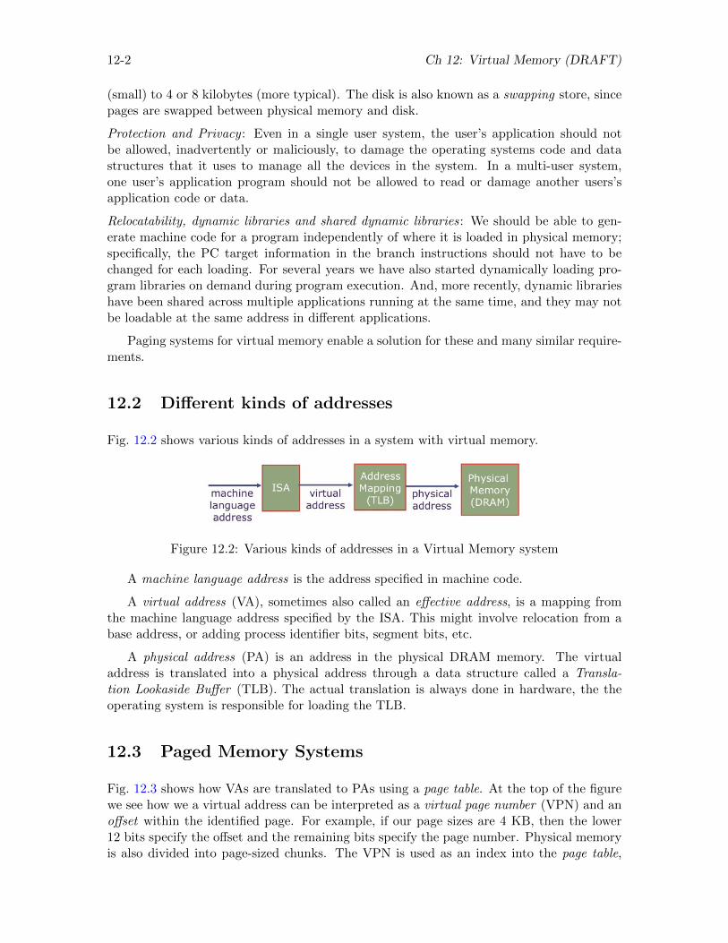
12-2 Ch 12: Virtual Memory (DRAFT)
(small) to 4 or 8 kilobytes (more typical). The disk is also known as a swapping store, sincepages are swapped between physical memory and disk.
Protection and Privacy : Even in a single user system, the user’s application should notbe allowed, inadvertently or maliciously, to damage the operating systems code and datastructures that it uses to manage all the devices in the system. In a multi-user system,one user’s application program should not be allowed to read or damage another users’sapplication code or data.
Relocatability, dynamic libraries and shared dynamic libraries: We should be able to gen-erate machine code for a program independently of where it is loaded in physical memory;specifically, the PC target information in the branch instructions should not have to bechanged for each loading. For several years we have also started dynamically loading pro-gram libraries on demand during program execution. And, more recently, dynamic librarieshave been shared across multiple applications running at the same time, and they may notbe loadable at the same address in different applications.
Paging systems for virtual memory enable a solution for these and many similar require-ments.
12.2 Different kinds of addresses
Fig. 12.2 shows various kinds of addresses in a system with virtual memory.
Figure 12.2: Various kinds of addresses in a Virtual Memory system
A machine language address is the address specified in machine code.
A virtual address (VA), sometimes also called an effective address, is a mapping fromthe machine language address specified by the ISA. This might involve relocation from abase address, or adding process identifier bits, segment bits, etc.
A physical address (PA) is an address in the physical DRAM memory. The virtualaddress is translated into a physical address through a data structure called a Transla-tion Lookaside Buffer (TLB). The actual translation is always done in hardware, the theoperating system is responsible for loading the TLB.
12.3 Paged Memory Systems
Fig. 12.3 shows how VAs are translated to PAs using a page table. At the top of the figurewe see how we a virtual address can be interpreted as a virtual page number (VPN) and anoffset within the identified page. For example, if our page sizes are 4 KB, then the lower12 bits specify the offset and the remaining bits specify the page number. Physical memoryis also divided into page-sized chunks. The VPN is used as an index into the page table,
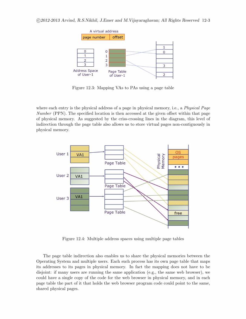
c©2012-2013 Arvind, R.S.Nikhil, J.Emer and M.Vijayaraghavan; All Rights Reserved 12-3
Figure 12.3: Mapping VAs to PAs using a page table
where each entry is the physical address of a page in physical memory, i.e., a Physical PageNumber (PPN). The specified location is then accessed at the given offset within that pageof physical memory. As suggested by the criss-crossing lines in the diagram, this level ofindirection through the page table also allows us to store virtual pages non-contiguously inphysical memory.
Figure 12.4: Multiple address spaces using multiple page tables
The page table indirection also enables us to share the physical memories between theOperating System and multiple users. Each such process has its own page table that mapsits addresses to its pages in physical memory. In fact the mapping does not have to bedisjoint: if many users are running the same application (e.g., the same web browser), wecould have a single copy of the code for the web browser in physical memory, and in eachpage table the part of it that holds the web browser program code could point to the same,shared physical pages.
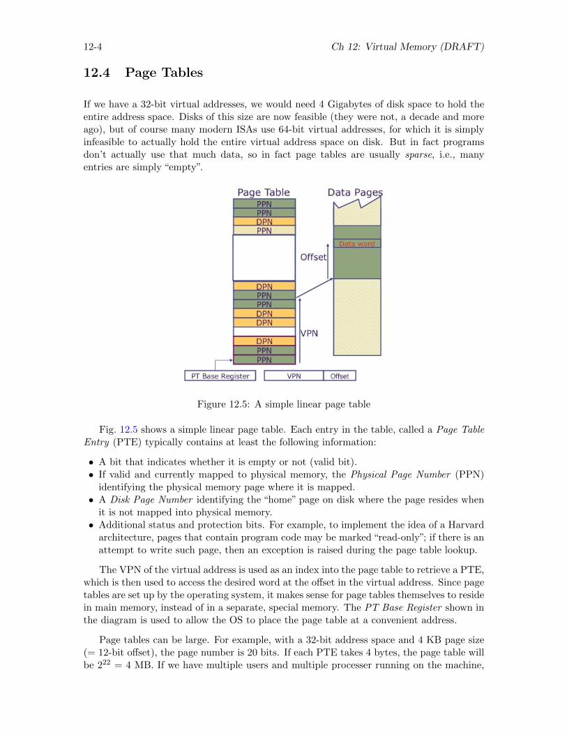
12-4 Ch 12: Virtual Memory (DRAFT)
12.4 Page Tables
If we have a 32-bit virtual addresses, we would need 4 Gigabytes of disk space to hold theentire address space. Disks of this size are now feasible (they were not, a decade and moreago), but of course many modern ISAs use 64-bit virtual addresses, for which it is simplyinfeasible to actually hold the entire virtual address space on disk. But in fact programsdon’t actually use that much data, so in fact page tables are usually sparse, i.e., manyentries are simply “empty”.
Figure 12.5: A simple linear page table
Fig. 12.5 shows a simple linear page table. Each entry in the table, called a Page TableEntry (PTE) typically contains at least the following information:
• A bit that indicates whether it is empty or not (valid bit).• If valid and currently mapped to physical memory, the Physical Page Number (PPN)
identifying the physical memory page where it is mapped.• A Disk Page Number identifying the “home” page on disk where the page resides when
it is not mapped into physical memory.• Additional status and protection bits. For example, to implement the idea of a Harvard
architecture, pages that contain program code may be marked “read-only”; if there is anattempt to write such page, then an exception is raised during the page table lookup.
The VPN of the virtual address is used as an index into the page table to retrieve a PTE,which is then used to access the desired word at the offset in the virtual address. Since pagetables are set up by the operating system, it makes sense for page tables themselves to residein main memory, instead of in a separate, special memory. The PT Base Register shown inthe diagram is used to allow the OS to place the page table at a convenient address.
Page tables can be large. For example, with a 32-bit address space and 4 KB page size(= 12-bit offset), the page number is 20 bits. If each PTE takes 4 bytes, the page table willbe 222 = 4 MB. If we have multiple users and multiple processer running on the machine,
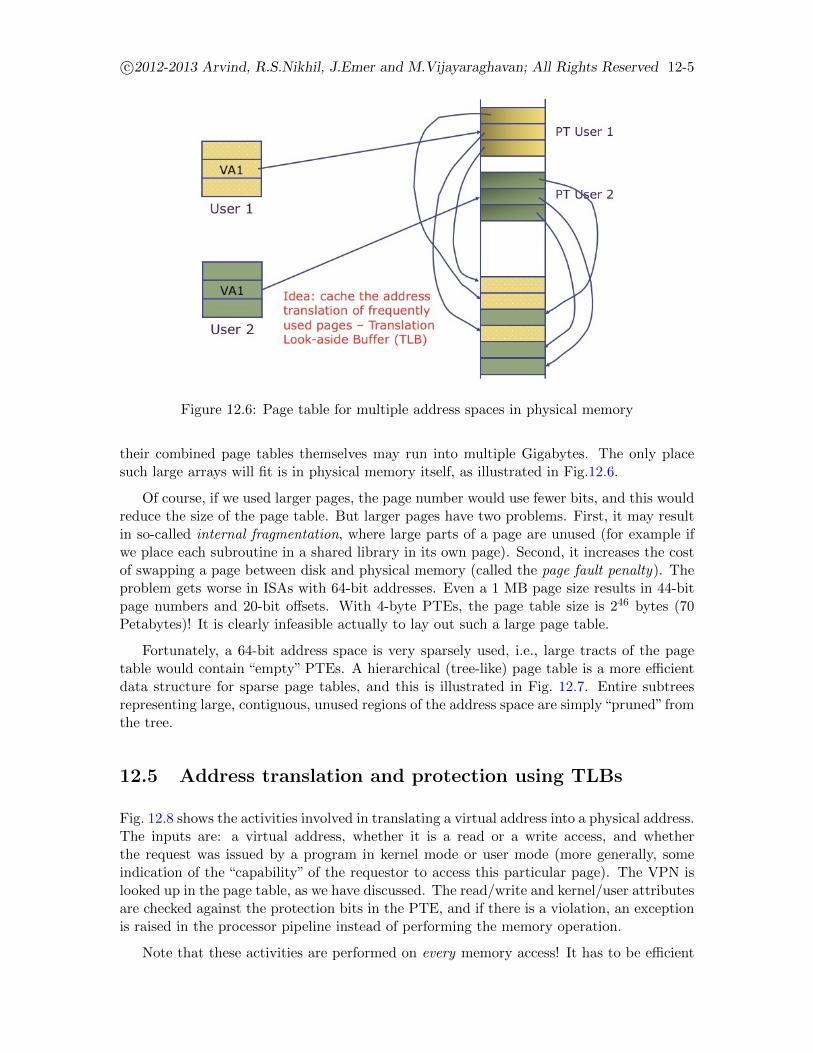
c©2012-2013 Arvind, R.S.Nikhil, J.Emer and M.Vijayaraghavan; All Rights Reserved 12-5
Figure 12.6: Page table for multiple address spaces in physical memory
their combined page tables themselves may run into multiple Gigabytes. The only placesuch large arrays will fit is in physical memory itself, as illustrated in Fig.12.6.
Of course, if we used larger pages, the page number would use fewer bits, and this wouldreduce the size of the page table. But larger pages have two problems. First, it may resultin so-called internal fragmentation, where large parts of a page are unused (for example ifwe place each subroutine in a shared library in its own page). Second, it increases the costof swapping a page between disk and physical memory (called the page fault penalty). Theproblem gets worse in ISAs with 64-bit addresses. Even a 1 MB page size results in 44-bitpage numbers and 20-bit offsets. With 4-byte PTEs, the page table size is 246 bytes (70Petabytes)! It is clearly infeasible actually to lay out such a large page table.
Fortunately, a 64-bit address space is very sparsely used, i.e., large tracts of the pagetable would contain “empty” PTEs. A hierarchical (tree-like) page table is a more efficientdata structure for sparse page tables, and this is illustrated in Fig. 12.7. Entire subtreesrepresenting large, contiguous, unused regions of the address space are simply“pruned” fromthe tree.
12.5 Address translation and protection using TLBs
Fig. 12.8 shows the activities involved in translating a virtual address into a physical address.The inputs are: a virtual address, whether it is a read or a write access, and whetherthe request was issued by a program in kernel mode or user mode (more generally, someindication of the “capability” of the requestor to access this particular page). The VPN islooked up in the page table, as we have discussed. The read/write and kernel/user attributesare checked against the protection bits in the PTE, and if there is a violation, an exceptionis raised in the processor pipeline instead of performing the memory operation.
Note that these activities are performed on every memory access! It has to be efficient

12-6 Ch 12: Virtual Memory (DRAFT)
Figure 12.7: Hierarchical page tables for large, sparse address spaces
Figure 12.8: Address translation and protection
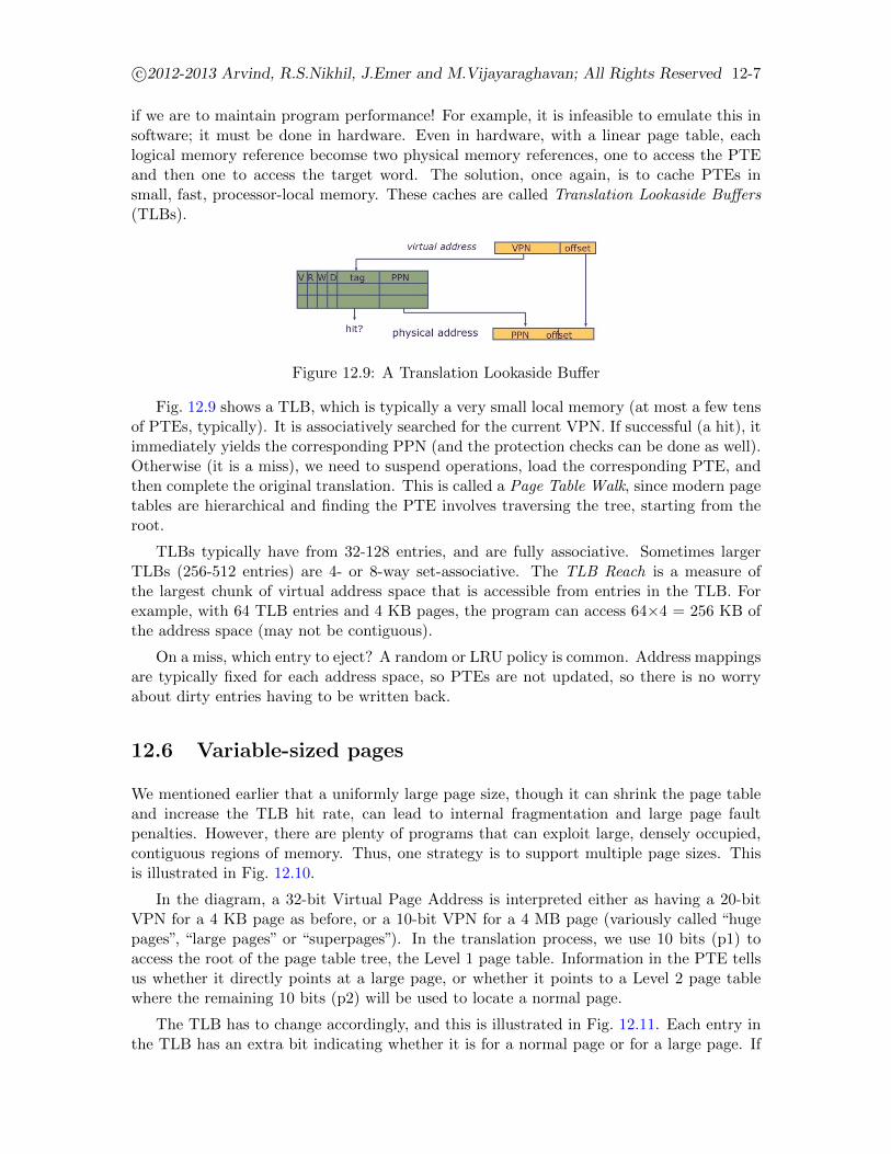
c©2012-2013 Arvind, R.S.Nikhil, J.Emer and M.Vijayaraghavan; All Rights Reserved 12-7
if we are to maintain program performance! For example, it is infeasible to emulate this insoftware; it must be done in hardware. Even in hardware, with a linear page table, eachlogical memory reference becomse two physical memory references, one to access the PTEand then one to access the target word. The solution, once again, is to cache PTEs insmall, fast, processor-local memory. These caches are called Translation Lookaside Buffers(TLBs).
Figure 12.9: A Translation Lookaside Buffer
Fig. 12.9 shows a TLB, which is typically a very small local memory (at most a few tensof PTEs, typically). It is associatively searched for the current VPN. If successful (a hit), itimmediately yields the corresponding PPN (and the protection checks can be done as well).Otherwise (it is a miss), we need to suspend operations, load the corresponding PTE, andthen complete the original translation. This is called a Page Table Walk, since modern pagetables are hierarchical and finding the PTE involves traversing the tree, starting from theroot.
TLBs typically have from 32-128 entries, and are fully associative. Sometimes largerTLBs (256-512 entries) are 4- or 8-way set-associative. The TLB Reach is a measure ofthe largest chunk of virtual address space that is accessible from entries in the TLB. Forexample, with 64 TLB entries and 4 KB pages, the program can access 64×4 = 256 KB ofthe address space (may not be contiguous).
On a miss, which entry to eject? A random or LRU policy is common. Address mappingsare typically fixed for each address space, so PTEs are not updated, so there is no worryabout dirty entries having to be written back.
12.6 Variable-sized pages
We mentioned earlier that a uniformly large page size, though it can shrink the page tableand increase the TLB hit rate, can lead to internal fragmentation and large page faultpenalties. However, there are plenty of programs that can exploit large, densely occupied,contiguous regions of memory. Thus, one strategy is to support multiple page sizes. Thisis illustrated in Fig. 12.10.
In the diagram, a 32-bit Virtual Page Address is interpreted either as having a 20-bitVPN for a 4 KB page as before, or a 10-bit VPN for a 4 MB page (variously called “hugepages”, “large pages” or “superpages”). In the translation process, we use 10 bits (p1) toaccess the root of the page table tree, the Level 1 page table. Information in the PTE tellsus whether it directly points at a large page, or whether it points to a Level 2 page tablewhere the remaining 10 bits (p2) will be used to locate a normal page.
The TLB has to change accordingly, and this is illustrated in Fig. 12.11. Each entry inthe TLB has an extra bit indicating whether it is for a normal page or for a large page. If
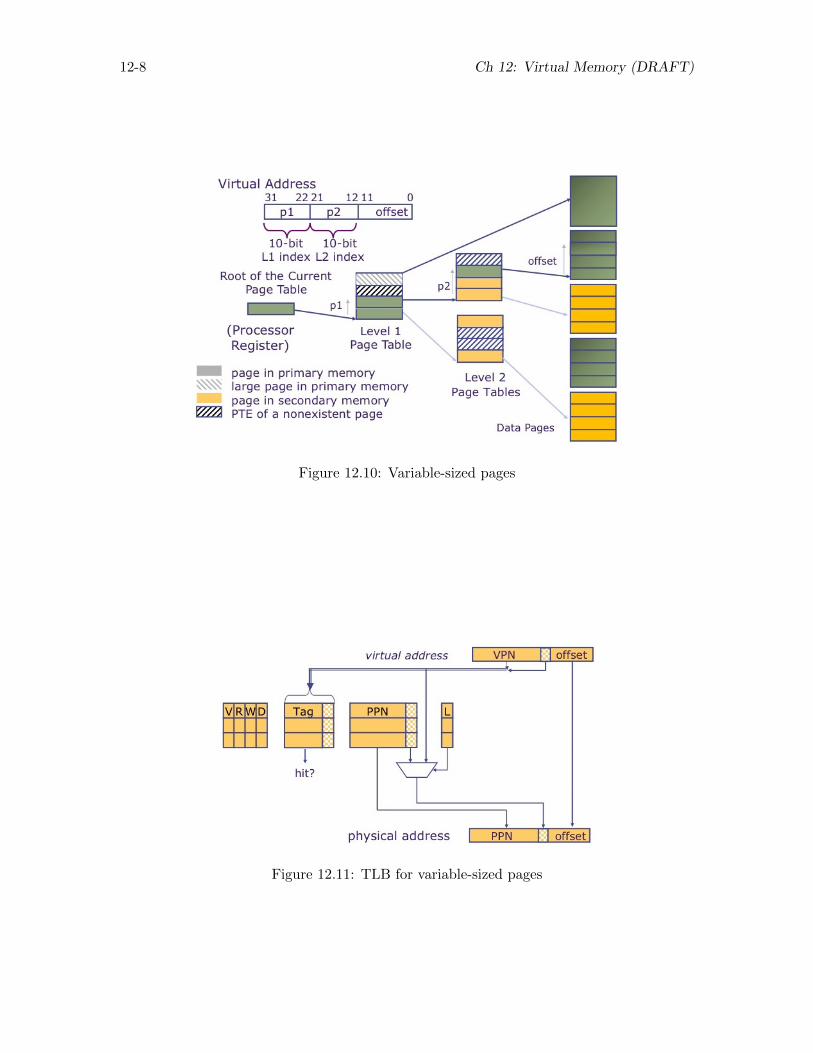
12-8 Ch 12: Virtual Memory (DRAFT)
Figure 12.10: Variable-sized pages
Figure 12.11: TLB for variable-sized pages
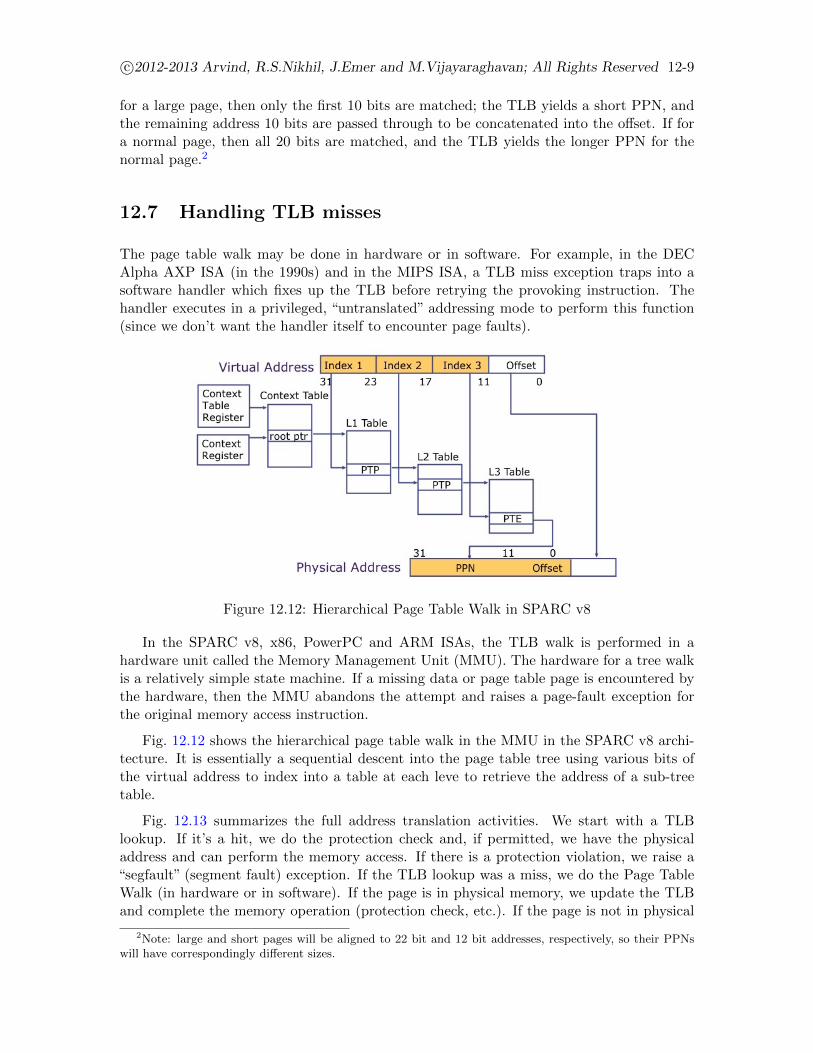
c©2012-2013 Arvind, R.S.Nikhil, J.Emer and M.Vijayaraghavan; All Rights Reserved 12-9
for a large page, then only the first 10 bits are matched; the TLB yields a short PPN, andthe remaining address 10 bits are passed through to be concatenated into the offset. If fora normal page, then all 20 bits are matched, and the TLB yields the longer PPN for thenormal page.2
12.7 Handling TLB misses
The page table walk may be done in hardware or in software. For example, in the DECAlpha AXP ISA (in the 1990s) and in the MIPS ISA, a TLB miss exception traps into asoftware handler which fixes up the TLB before retrying the provoking instruction. Thehandler executes in a privileged, “untranslated” addressing mode to perform this function(since we don’t want the handler itself to encounter page faults).
Figure 12.12: Hierarchical Page Table Walk in SPARC v8
In the SPARC v8, x86, PowerPC and ARM ISAs, the TLB walk is performed in ahardware unit called the Memory Management Unit (MMU). The hardware for a tree walkis a relatively simple state machine. If a missing data or page table page is encountered bythe hardware, then the MMU abandons the attempt and raises a page-fault exception forthe original memory access instruction.
Fig. 12.12 shows the hierarchical page table walk in the MMU in the SPARC v8 archi-tecture. It is essentially a sequential descent into the page table tree using various bits ofthe virtual address to index into a table at each leve to retrieve the address of a sub-treetable.
Fig. 12.13 summarizes the full address translation activities. We start with a TLBlookup. If it’s a hit, we do the protection check and, if permitted, we have the physicaladdress and can perform the memory access. If there is a protection violation, we raise a“segfault” (segment fault) exception. If the TLB lookup was a miss, we do the Page TableWalk (in hardware or in software). If the page is in physical memory, we update the TLBand complete the memory operation (protection check, etc.). If the page is not in physical
2Note: large and short pages will be aligned to 22 bit and 12 bit addresses, respectively, so their PPNswill have correspondingly different sizes.
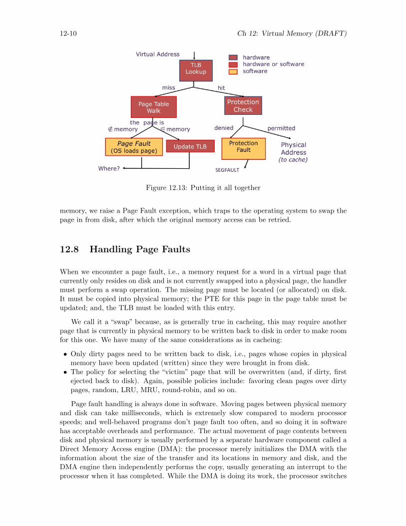
12-10 Ch 12: Virtual Memory (DRAFT)
Figure 12.13: Putting it all together
memory, we raise a Page Fault exception, which traps to the operating system to swap thepage in from disk, after which the original memory access can be retried.
12.8 Handling Page Faults
When we encounter a page fault, i.e., a memory request for a word in a virtual page thatcurrently only resides on disk and is not currently swapped into a physical page, the handlermust perform a swap operation. The missing page must be located (or allocated) on disk.It must be copied into physical memory; the PTE for this page in the page table must beupdated; and, the TLB must be loaded with this entry.
We call it a “swap” because, as is generally true in cacheing, this may require anotherpage that is currently in physical memory to be written back to disk in order to make roomfor this one. We have many of the same considerations as in cacheing:
• Only dirty pages need to be written back to disk, i.e., pages whose copies in physicalmemory have been updated (written) since they were brought in from disk.• The policy for selecting the “victim” page that will be overwritten (and, if dirty, first
ejected back to disk). Again, possible policies include: favoring clean pages over dirtypages, random, LRU, MRU, round-robin, and so on.
Page fault handling is always done in software. Moving pages between physical memoryand disk can take milliseconds, which is extremely slow compared to modern processorspeeds; and well-behaved programs don’t page fault too often, and so doing it in softwarehas acceptable overheads and performance. The actual movement of page contents betweendisk and physical memory is usually performed by a separate hardware component called aDirect Memory Access engine (DMA): the processor merely initializes the DMA with theinformation about the size of the transfer and its locations in memory and disk, and theDMA engine then independently performs the copy, usually generating an interrupt to theprocessor when it has completed. While the DMA is doing its work, the processor switches
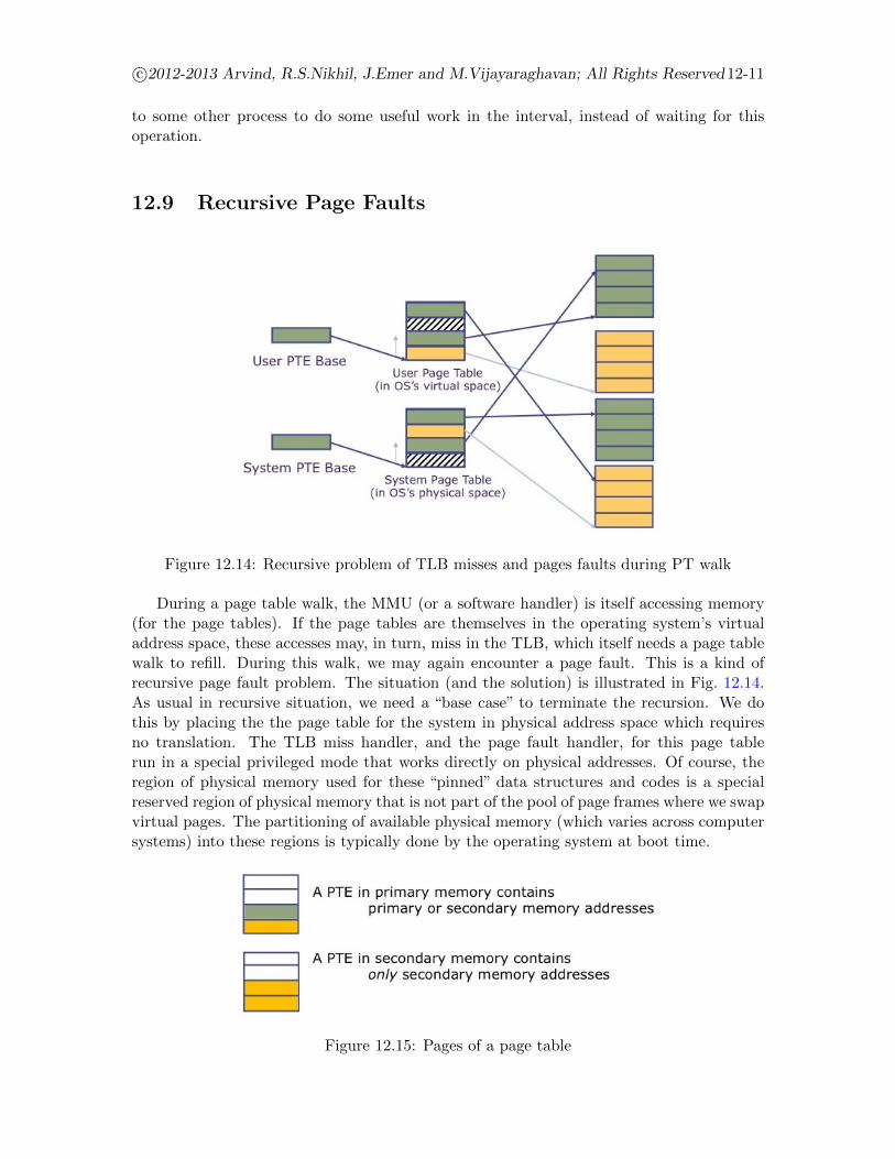
c©2012-2013 Arvind, R.S.Nikhil, J.Emer and M.Vijayaraghavan; All Rights Reserved12-11
to some other process to do some useful work in the interval, instead of waiting for thisoperation.
12.9 Recursive Page Faults
Figure 12.14: Recursive problem of TLB misses and pages faults during PT walk
During a page table walk, the MMU (or a software handler) is itself accessing memory(for the page tables). If the page tables are themselves in the operating system’s virtualaddress space, these accesses may, in turn, miss in the TLB, which itself needs a page tablewalk to refill. During this walk, we may again encounter a page fault. This is a kind ofrecursive page fault problem. The situation (and the solution) is illustrated in Fig. 12.14.As usual in recursive situation, we need a “base case” to terminate the recursion. We dothis by placing the the page table for the system in physical address space which requiresno translation. The TLB miss handler, and the page fault handler, for this page tablerun in a special privileged mode that works directly on physical addresses. Of course, theregion of physical memory used for these “pinned” data structures and codes is a specialreserved region of physical memory that is not part of the pool of page frames where we swapvirtual pages. The partitioning of available physical memory (which varies across computersystems) into these regions is typically done by the operating system at boot time.
Figure 12.15: Pages of a page table
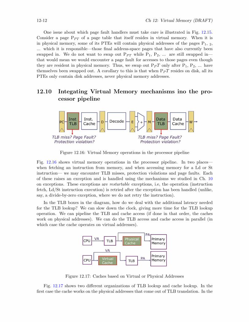
12-12 Ch 12: Virtual Memory (DRAFT)
One issue about which page fault handlers must take care is illustrated in Fig. 12.15.Consider a page PPT of a page table that itself resides in virtual memory. When it isin physical memory, some of its PTEs will contain physical addresses of the pages P1, 2,... which it is responsible—those final address-space pages that have also currently beenswapped in. We do not want to swap out PPT while P1, P2, ... are still swapped in—that would mean we would encounter a page fault for accesses to those pages even thoughthey are resident in physical memory. Thus, we swap out PPT only after P1, P2, ... havethemselves been swapped out. A corollary to this is that when PPT resides on disk, all itsPTEs only contain disk addresses, never physical memory addresses.
12.10 Integating Virtual Memory mechanisms ino the pro-cessor pipeline
Figure 12.16: Virtual Memory operations in the processor pipeline
Fig. 12.16 shows virtual memory operations in the processor pipeline. In two places—when fetching an instruction from memory, and when accessing memory for a Ld or Stinstruction— we may encounter TLB misses, protection violations and page faults. Eachof these raises an exception and is handled using the mechanisms we studied in Ch. 10on exceptions. These exceptions are restartable exceptions, i.e, the operation (instructionfetch, Ld/St instruction execution) is retried after the exception has been handled (unlike,say, a divide-by-zero exception, where we do not retry the instruction).
In the TLB boxes in the diagram, how do we deal with the additional latency neededfor the TLB lookup? We can slow down the clock, giving more time for the TLB lookupoperation. We can pipeline the TLB and cache access (if done in that order, the cacheswork on physical addresses). We can do the TLB access and cache access in parallel (inwhich case the cache operates on virtual addresses).
Figure 12.17: Caches based on Virtual or Physical Addresses
Fig. 12.17 shows two different organizations of TLB lookup and cache lookup. In thefirst case the cache works on the physical addresses that come out of TLB translation. In the
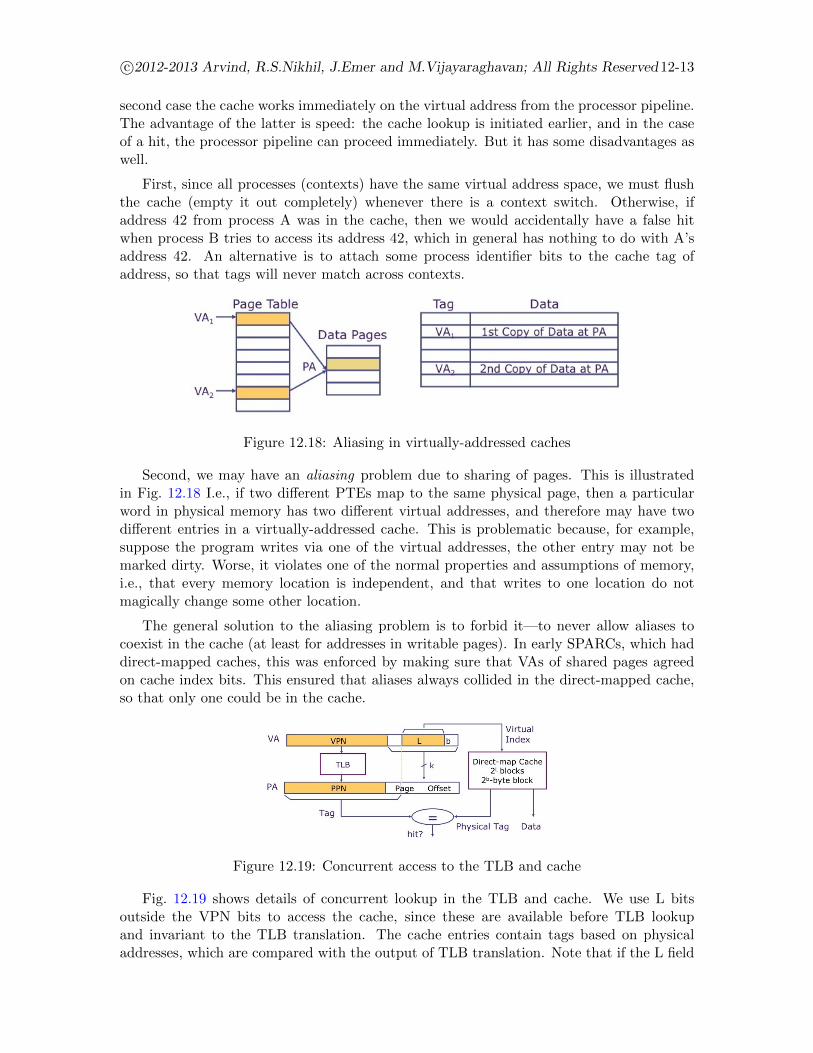
c©2012-2013 Arvind, R.S.Nikhil, J.Emer and M.Vijayaraghavan; All Rights Reserved12-13
second case the cache works immediately on the virtual address from the processor pipeline.The advantage of the latter is speed: the cache lookup is initiated earlier, and in the caseof a hit, the processor pipeline can proceed immediately. But it has some disadvantages aswell.
First, since all processes (contexts) have the same virtual address space, we must flushthe cache (empty it out completely) whenever there is a context switch. Otherwise, ifaddress 42 from process A was in the cache, then we would accidentally have a false hitwhen process B tries to access its address 42, which in general has nothing to do with A’saddress 42. An alternative is to attach some process identifier bits to the cache tag ofaddress, so that tags will never match across contexts.
Figure 12.18: Aliasing in virtually-addressed caches
Second, we may have an aliasing problem due to sharing of pages. This is illustratedin Fig. 12.18 I.e., if two different PTEs map to the same physical page, then a particularword in physical memory has two different virtual addresses, and therefore may have twodifferent entries in a virtually-addressed cache. This is problematic because, for example,suppose the program writes via one of the virtual addresses, the other entry may not bemarked dirty. Worse, it violates one of the normal properties and assumptions of memory,i.e., that every memory location is independent, and that writes to one location do notmagically change some other location.
The general solution to the aliasing problem is to forbid it—to never allow aliases tocoexist in the cache (at least for addresses in writable pages). In early SPARCs, which haddirect-mapped caches, this was enforced by making sure that VAs of shared pages agreedon cache index bits. This ensured that aliases always collided in the direct-mapped cache,so that only one could be in the cache.
Figure 12.19: Concurrent access to the TLB and cache
Fig. 12.19 shows details of concurrent lookup in the TLB and cache. We use L bitsoutside the VPN bits to access the cache, since these are available before TLB lookupand invariant to the TLB translation. The cache entries contain tags based on physicaladdresses, which are compared with the output of TLB translation. Note that if the L field
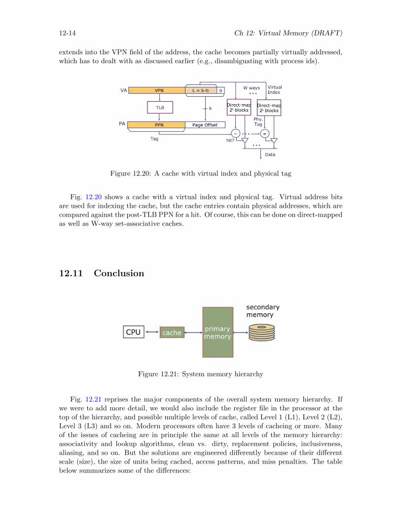
12-14 Ch 12: Virtual Memory (DRAFT)
extends into the VPN field of the address, the cache becomes partially virtually addressed,which has to dealt with as discussed earlier (e.g., disambiguating with process ids).
Figure 12.20: A cache with virtual index and physical tag
Fig. 12.20 shows a cache with a virtual index and physical tag. Virtual address bitsare used for indexing the cache, but the cache entries contain physical addresses, which arecompared against the post-TLB PPN for a hit. Of course, this can be done on direct-mappedas well as W-way set-associative caches.
12.11 Conclusion
Figure 12.21: System memory hierarchy
Fig. 12.21 reprises the major components of the overall system memory hierarchy. Ifwe were to add more detail, we would also include the register file in the processor at thetop of the hierarchy, and possible multiple levels of cache, called Level 1 (L1), Level 2 (L2),Level 3 (L3) and so on. Modern processors often have 3 levels of cacheing or more. Manyof the issues of cacheing are in principle the same at all levels of the memory hierarchy:associativity and lookup algorithms, clean vs. dirty, replacement policies, inclusiveness,aliasing, and so on. But the solutions are engineered differently because of their differentscale (size), the size of units being cached, access patterns, and miss penalties. The tablebelow summarizes some of the differences:
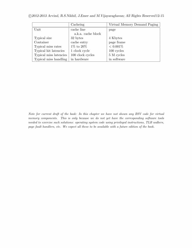
c©2012-2013 Arvind, R.S.Nikhil, J.Emer and M.Vijayaraghavan; All Rights Reserved12-15
Cacheing Virtual Memory Demand Paging
Unit cache line pagea.k.a. cache block
Typical size 32 bytes 4 KbytesContainer cache entry page frameTypical miss rates 1% to 20% < 0.001%Typical hit latencies 1 clock cycle 100 cyclesTypical miss latencies 100 clock cycles 5 M cyclesTypical miss handling in hardware in software
Note for current draft of the book: In this chapter we have not shown any BSV code for virtual
memory components. This is only because we do not yet have the corresponding software tools
needed to exercise such solutions: operating system code using privileged instructions, TLB walkers,
page fault handlers, etc. We expect all these to be available with a future edition of the book.

12-16 Ch 12: Virtual Memory (DRAFT)
Chapter 13
Future Topics
This chapter lists a number of potential topics for future editions of this book.
13.1 Asynchronous Exceptions and Interrupts
13.2 Out-of-order pipelines
Register renaming, data flow. Precise exceptions.
13.3 Protection and System Issues
Protection issues and solutions. Virtualization. Capabilities.
13.4 I and D Cache Coherence
The coherence problem between Instruction and Data memories when Instruction memoryis modifiable. Princeton architecture. Self-modifying code. On-the-fly optimization. JITcompiling. Binary translation.
13.5 Multicore and Multicore cache coherence
Multicore, SMPs.
Memory models and memory ordering semantics.
Multicore and directory-based cache coherence.
Synchronization primitives. Transactional memory.
13-1
13-2 Ch 13: Possible Remaining Topics (DRAFT)
13.6 Simultaneous Multithreading
SMT
13.7 Energy efficiency
Power and power management.
13.8 Hardware accelerators
Extending an ISA with HW-accelerated op codes, implemented in FPGAs or ASICs
Appendix A
SMIPS Reference
SMIPS (“Simple MIPS”) is a subset of the full MIPS instruction set architecture (ISA). MIPSwas one of the first commercial RISC (Reduced Instruction Set Computer) processors, andgrew out of the earlier MIPS research project at Stanford University. MIPS originally stoodfor “Microprocessor without Interlocking Pipeline Stages” and the goal was to simplify themachine pipeline by requiring the compiler to schedule around pipeline hazards includinga branch delay slot and a load delay slot (although those particular architectural choiceshave been abandoned). Today, MIPS CPUs are used in a wide range of devices: Casiobuilds handheld PDAs using MIPS CPUs, Sony uses two MIPS CPUs in the Playstation-2, many Cisco internet routers contain MIPS CPUs, and Silicon Graphics makes Originsupercomputers containing up to 512 MIPS processors sharing a common memory. MIPSimplementations probably span the widest range for any commercial ISA, from simple single-issue in-order pipelines to quad-issue out-of-order superscalar processors.
There are several variants of the MIPS ISA. The ISA has evolved from the original32-bit MIPS-I architecture used in the MIPS R2000 processor which appeared in 1986. TheMIPS-II architecture added a few more instructions while retaining a 32-bit address space.The MIPS-II architecture also added hardware interlocks for the load delay slot. In practice,compilers couldn’t fill enough of the load delay slots with useful work and the NOPs in theload delay slots wasted instruction cache space. (Removing the branch delay slots might alsohave been a good idea, but would have required a second set of branch instruction encodingsto remain backwards compatible.) The MIPS-III architecture debuted with the MIPS R4000processor, and this extended the address space to 64 bits while leaving the original 32-bit architecture as a proper subset. The MIPS-IV architecture was developed by SiliconGraphics to add many enhancements for floating-point computations and appeared first inthe MIPS R8000 and later in the MIPS R10000. Over time, the MIPS architecture has beenwidely extended, occasionally in non-compatible ways, by different processor implementors.MIPS Technologies, the current owners of the architecture, are trying to rationalize thearchitecture into two broad groupings: MIPS32 is the 32-bit address space version, MIPS64is the 64-bit address space version. There is also MIPS16, which is a compact encoding ofMIPS32 that only uses 16 bits for each instruction. You can find a complete descriptionof the MIPS instruction set at the MIPS Technologies web site [5] or in the book by Kaneand Heinrich [6]. The book by Sweetman also explains MIPS programming [8]. Anothersource of MIPS details and implementation ideas is “Computer Organization and Design:The Hardware/Software Interface” [3].
SMIPS-1
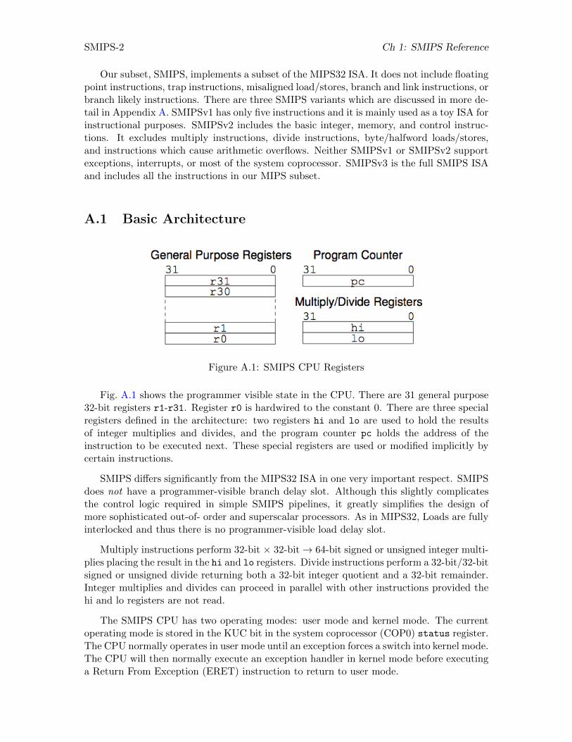
SMIPS-2 Ch 1: SMIPS Reference
Our subset, SMIPS, implements a subset of the MIPS32 ISA. It does not include floatingpoint instructions, trap instructions, misaligned load/stores, branch and link instructions, orbranch likely instructions. There are three SMIPS variants which are discussed in more de-tail in Appendix A. SMIPSv1 has only five instructions and it is mainly used as a toy ISA forinstructional purposes. SMIPSv2 includes the basic integer, memory, and control instruc-tions. It excludes multiply instructions, divide instructions, byte/halfword loads/stores,and instructions which cause arithmetic overflows. Neither SMIPSv1 or SMIPSv2 supportexceptions, interrupts, or most of the system coprocessor. SMIPSv3 is the full SMIPS ISAand includes all the instructions in our MIPS subset.
A.1 Basic Architecture
Figure A.1: SMIPS CPU Registers
Fig. A.1 shows the programmer visible state in the CPU. There are 31 general purpose32-bit registers r1-r31. Register r0 is hardwired to the constant 0. There are three specialregisters defined in the architecture: two registers hi and lo are used to hold the resultsof integer multiplies and divides, and the program counter pc holds the address of theinstruction to be executed next. These special registers are used or modified implicitly bycertain instructions.
SMIPS differs significantly from the MIPS32 ISA in one very important respect. SMIPSdoes not have a programmer-visible branch delay slot. Although this slightly complicatesthe control logic required in simple SMIPS pipelines, it greatly simplifies the design ofmore sophisticated out-of- order and superscalar processors. As in MIPS32, Loads are fullyinterlocked and thus there is no programmer-visible load delay slot.
Multiply instructions perform 32-bit × 32-bit→ 64-bit signed or unsigned integer multi-plies placing the result in the hi and lo registers. Divide instructions perform a 32-bit/32-bitsigned or unsigned divide returning both a 32-bit integer quotient and a 32-bit remainder.Integer multiplies and divides can proceed in parallel with other instructions provided thehi and lo registers are not read.
The SMIPS CPU has two operating modes: user mode and kernel mode. The currentoperating mode is stored in the KUC bit in the system coprocessor (COP0) status register.The CPU normally operates in user mode until an exception forces a switch into kernel mode.The CPU will then normally execute an exception handler in kernel mode before executinga Return From Exception (ERET) instruction to return to user mode.

SMIPS-3
A.2 System Control Coprocessor (CP0)
The SMIPS system control coprocessor contains a number of registers used for exceptionhandling, communication with a test rig, and the counter/timer. These registers are readand written using the MIPS standard MFC0 and MTC0 instructions respectively. Usermode can access the system control coprocessor only if the cu[0] bit is set in the statusregister. Kernel mode can always access CP0, regardless of the setting of the cu[0] bit.CP0 control registers are listed in Table A.1.
Number Register Description
0-7 unused8 badvaddr Bad virtual address.9 count Counter/timer register.10 unused11 compare Timer compare register.12 status Status register.13 cause Cause of last exception.14 epc Exception program counter.
15-19 unused20 fromhost Test input register.21 tohost Test output register.
22-31 unused
Table A.1: CP0 control registers
A.2.1 Test Communication Registers
Figure A.2: Fromhost and Tohost Register Formats
There are two registers used for communicating and synchronizing with an external hosttest system. Typically, these will be accessed over a scan chain. The fromhost register isan 8-bit read only register that contains a value written by the host system. The tohost
register is an 8-bit read/write register that contains a value that can be read back by thehost system. The tohost register is cleared by reset to simplify synchronization with thehost test rig. Their format is shown in Fig. A.2.
A.2.2 Counter/Timer Registers
SMIPS includes a counter/timer facility provided by the two coprocessor 0 registers count
and compare. Both registers are 32 bits wide and are both readable and writeable. Theirformat is shown in Fig. A.3.
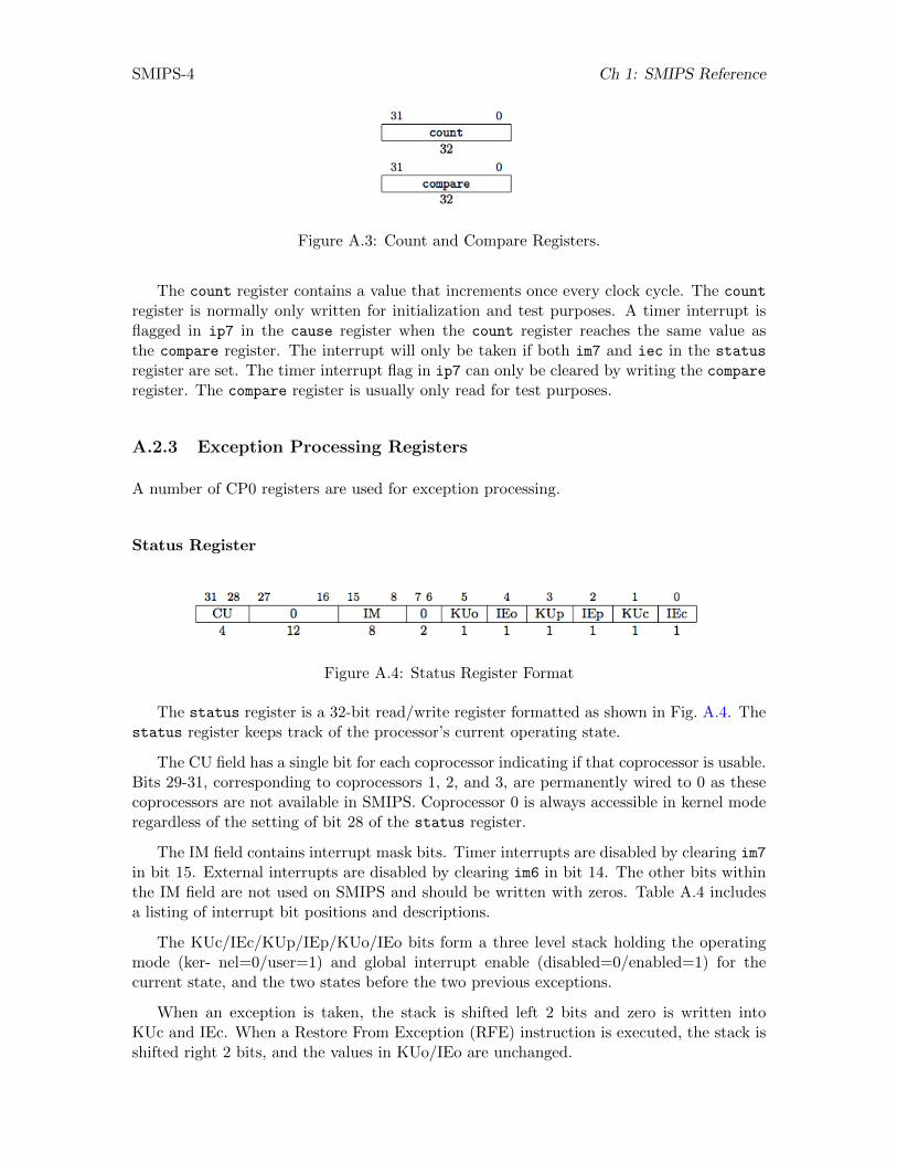
SMIPS-4 Ch 1: SMIPS Reference
Figure A.3: Count and Compare Registers.
The count register contains a value that increments once every clock cycle. The count
register is normally only written for initialization and test purposes. A timer interrupt isflagged in ip7 in the cause register when the count register reaches the same value asthe compare register. The interrupt will only be taken if both im7 and iec in the status
register are set. The timer interrupt flag in ip7 can only be cleared by writing the compare
register. The compare register is usually only read for test purposes.
A.2.3 Exception Processing Registers
A number of CP0 registers are used for exception processing.
Status Register
Figure A.4: Status Register Format
The status register is a 32-bit read/write register formatted as shown in Fig. A.4. Thestatus register keeps track of the processor’s current operating state.
The CU field has a single bit for each coprocessor indicating if that coprocessor is usable.Bits 29-31, corresponding to coprocessors 1, 2, and 3, are permanently wired to 0 as thesecoprocessors are not available in SMIPS. Coprocessor 0 is always accessible in kernel moderegardless of the setting of bit 28 of the status register.
The IM field contains interrupt mask bits. Timer interrupts are disabled by clearing im7
in bit 15. External interrupts are disabled by clearing im6 in bit 14. The other bits withinthe IM field are not used on SMIPS and should be written with zeros. Table A.4 includesa listing of interrupt bit positions and descriptions.
The KUc/IEc/KUp/IEp/KUo/IEo bits form a three level stack holding the operatingmode (ker- nel=0/user=1) and global interrupt enable (disabled=0/enabled=1) for thecurrent state, and the two states before the two previous exceptions.
When an exception is taken, the stack is shifted left 2 bits and zero is written intoKUc and IEc. When a Restore From Exception (RFE) instruction is executed, the stack isshifted right 2 bits, and the values in KUo/IEo are unchanged.
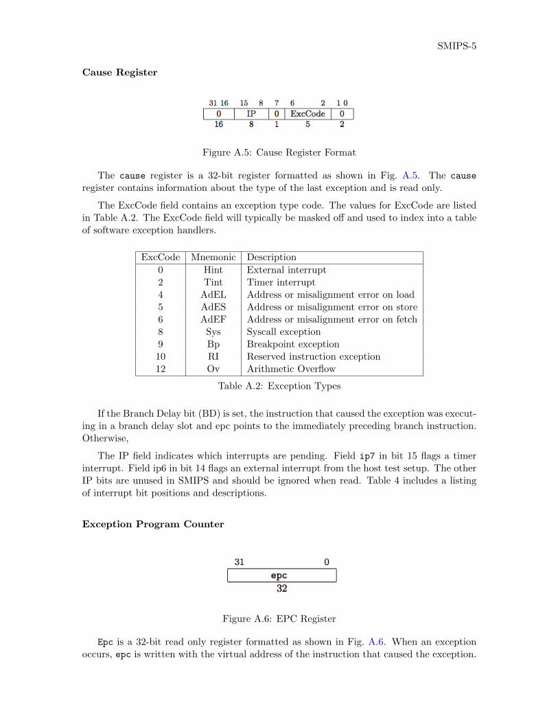
SMIPS-5
Cause Register
Figure A.5: Cause Register Format
The cause register is a 32-bit register formatted as shown in Fig. A.5. The cause
register contains information about the type of the last exception and is read only.
The ExcCode field contains an exception type code. The values for ExcCode are listedin Table A.2. The ExcCode field will typically be masked off and used to index into a tableof software exception handlers.
ExcCode Mnemonic Description
0 Hint External interrupt2 Tint Timer interrupt4 AdEL Address or misalignment error on load5 AdES Address or misalignment error on store6 AdEF Address or misalignment error on fetch8 Sys Syscall exception9 Bp Breakpoint exception10 RI Reserved instruction exception12 Ov Arithmetic Overflow
Table A.2: Exception Types
If the Branch Delay bit (BD) is set, the instruction that caused the exception was execut-ing in a branch delay slot and epc points to the immediately preceding branch instruction.Otherwise,
The IP field indicates which interrupts are pending. Field ip7 in bit 15 flags a timerinterrupt. Field ip6 in bit 14 flags an external interrupt from the host test setup. The otherIP bits are unused in SMIPS and should be ignored when read. Table 4 includes a listingof interrupt bit positions and descriptions.
Exception Program Counter
Figure A.6: EPC Register
Epc is a 32-bit read only register formatted as shown in Fig. A.6. When an exceptionoccurs, epc is written with the virtual address of the instruction that caused the exception.
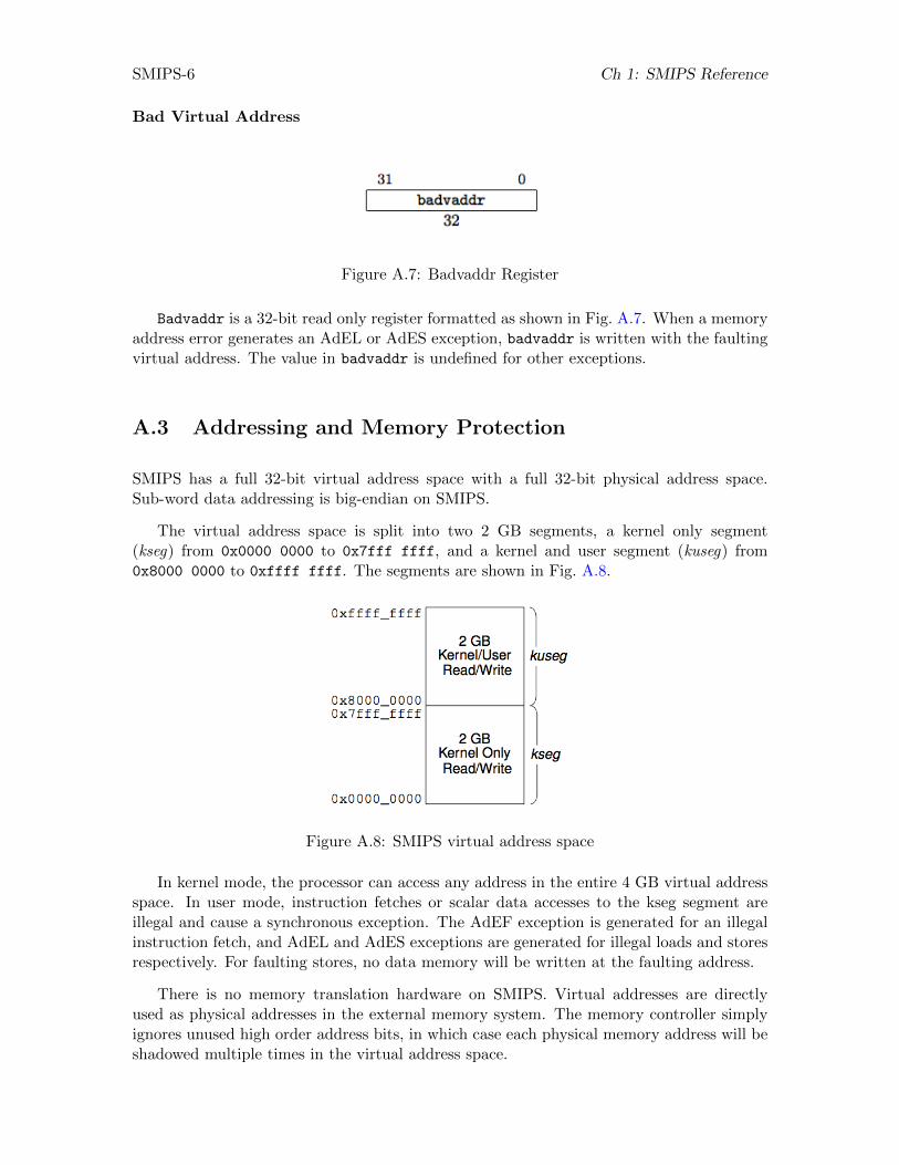
SMIPS-6 Ch 1: SMIPS Reference
Bad Virtual Address
Figure A.7: Badvaddr Register
Badvaddr is a 32-bit read only register formatted as shown in Fig. A.7. When a memoryaddress error generates an AdEL or AdES exception, badvaddr is written with the faultingvirtual address. The value in badvaddr is undefined for other exceptions.
A.3 Addressing and Memory Protection
SMIPS has a full 32-bit virtual address space with a full 32-bit physical address space.Sub-word data addressing is big-endian on SMIPS.
The virtual address space is split into two 2 GB segments, a kernel only segment(kseg) from 0x0000 0000 to 0x7fff ffff, and a kernel and user segment (kuseg) from0x8000 0000 to 0xffff ffff. The segments are shown in Fig. A.8.
Figure A.8: SMIPS virtual address space
In kernel mode, the processor can access any address in the entire 4 GB virtual addressspace. In user mode, instruction fetches or scalar data accesses to the kseg segment areillegal and cause a synchronous exception. The AdEF exception is generated for an illegalinstruction fetch, and AdEL and AdES exceptions are generated for illegal loads and storesrespectively. For faulting stores, no data memory will be written at the faulting address.
There is no memory translation hardware on SMIPS. Virtual addresses are directlyused as physical addresses in the external memory system. The memory controller simplyignores unused high order address bits, in which case each physical memory address will beshadowed multiple times in the virtual address space.
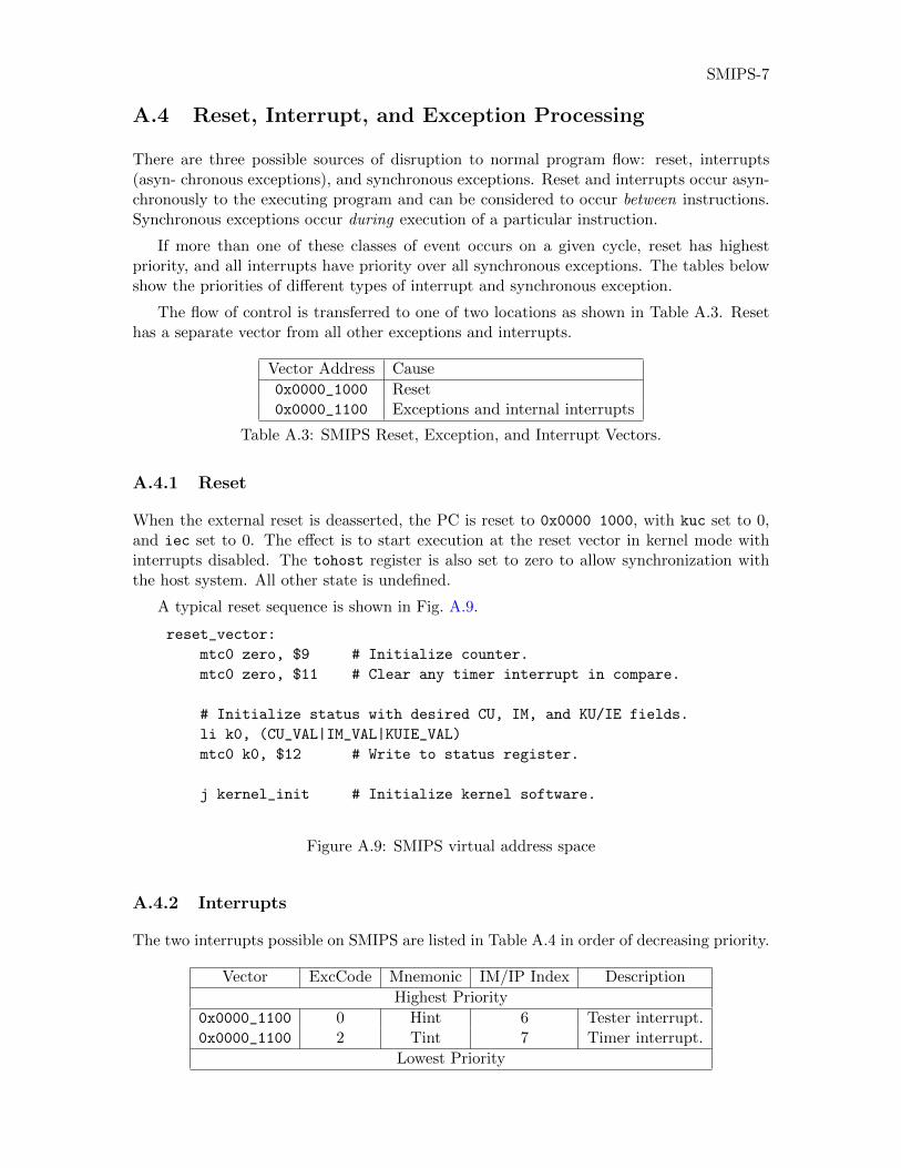
SMIPS-7
A.4 Reset, Interrupt, and Exception Processing
There are three possible sources of disruption to normal program flow: reset, interrupts(asyn- chronous exceptions), and synchronous exceptions. Reset and interrupts occur asyn-chronously to the executing program and can be considered to occur between instructions.Synchronous exceptions occur during execution of a particular instruction.
If more than one of these classes of event occurs on a given cycle, reset has highestpriority, and all interrupts have priority over all synchronous exceptions. The tables belowshow the priorities of different types of interrupt and synchronous exception.
The flow of control is transferred to one of two locations as shown in Table A.3. Resethas a separate vector from all other exceptions and interrupts.
Vector Address Cause
0x0000_1000 Reset0x0000_1100 Exceptions and internal interrupts
Table A.3: SMIPS Reset, Exception, and Interrupt Vectors.
A.4.1 Reset
When the external reset is deasserted, the PC is reset to 0x0000 1000, with kuc set to 0,and iec set to 0. The effect is to start execution at the reset vector in kernel mode withinterrupts disabled. The tohost register is also set to zero to allow synchronization withthe host system. All other state is undefined.
A typical reset sequence is shown in Fig. A.9.
reset_vector:
mtc0 zero, $9 # Initialize counter.
mtc0 zero, $11 # Clear any timer interrupt in compare.
# Initialize status with desired CU, IM, and KU/IE fields.
li k0, (CU_VAL|IM_VAL|KUIE_VAL)
mtc0 k0, $12 # Write to status register.
j kernel_init # Initialize kernel software.
Figure A.9: SMIPS virtual address space
A.4.2 Interrupts
The two interrupts possible on SMIPS are listed in Table A.4 in order of decreasing priority.
Vector ExcCode Mnemonic IM/IP Index Description
Highest Priority
0x0000_1100 0 Hint 6 Tester interrupt.0x0000_1100 2 Tint 7 Timer interrupt.
Lowest Priority

SMIPS-8 Ch 1: SMIPS Reference
Table A.4: SMIPS Interrupts.
All SMIPS interrupts are level triggered. For each interrupt there is an IP flag in thecause register that is set if that interrupt is pending, and an IM flag in the status registerthat enables the interrupt when set. In addition there is a single global interrupt enable bit,iec, that disables all interrupts if cleared. A particular interrupt can only occur if both IPand IM for that interrupt are set and iec is set, and there are no higher priority interrupts.
The host external interrupt flag IP6 can be written by the host test system over a scaninterface. Usually a protocol over the host scan interface informs the host that it can cleardown the interrupt flag.
The timer interrupt flag IP7 is set when the value in the count register matches thevalue in the compare register. The flag can only be cleared as a side-effect of a MTC0 writeto the compare register.
When an interrupt is taken, the PC is set to the interrupt vector, and the KU/IE stackin the status register is pushed two bits to the left, with KUc and IEc both cleared to 0.This starts the interrupt handler running in kernel mode with further interrupts disabled.The exccode field in the cause register is set to indicate the type of interrupt.
The epc register is loaded with a restart address. The epc address can be used to restartexecution after servicing the interrupt.
A.4.3 Synchronous Exceptions
Synchronous exceptions are listed in Table A.5 in order of decreasing priority.
ExcCode Mnemonic Description
Highest Priority
6 AdEF Address or misalignment error on fetch.10 RI Reserved instruction exception.8 Sys Syscall exception.9 Bp Breakpoint exception.12 Ov Arithmetic Overflow.4 AdEL Address or misalignment error on load.5 AdES Address or misalignment error on store.
Lowest Priority
Table A.5: SMIPS Synchronous Exceptions.
After a synchronous exception, the PC is set to 0x0000\_1100. The stack of kernel/userand interrupt enable bits held in the status register is pushed left two bits, and both kuc
and iec are set to 0.
The epc register is set to point to the instruction that caused the exception. Theexccode field in the cause register is set to indicate the type of exception.
If the exception was a coprocessor unusable exception (CpU), the ce field in the cause
register is set to the coprocessor number that caused the error. This field is undefined forother exceptions.

SMIPS-9
The overflow exception (Ov) can only occur for ADDI, ADD, and SUB instructions.
If the exception was an address error on a load or store (AdEL/AdES), the badvaddr
register is set to the faulting address. The value in badvaddr is undefined for other excep-tions.
All unimplemented and illegal instructions should cause a reserved instruction exception(RI).
A.5 Instruction Semantics and Encodings
SMIPS uses the standard MIPS instruction set.
A.5.1 Instruction Formats
There are three basic instruction formats, R-type, I-type, and J-type. These are a fixed 32bits in length, and must be aligned on a four-byte boundary in memory. An address errorexception (AdEF) is generated if the PC is misaligned on an instruction fetch.
R-Type
R-type instructions specify two source registers (rs and rt) and a destination register(rd). The 5-bit shamt field is used to specify shift immediate amounts and the 6-bit functcode is a second opcode field.
I-Type
I-type instructions specify one source register (rs) and a destination register (rt). Thesecond source operand is a sign or zero-extended 16-bit immediate. Logical immediateoperations use a zero-extended immediate, while all others use a sign-extended immediate.
J-Type
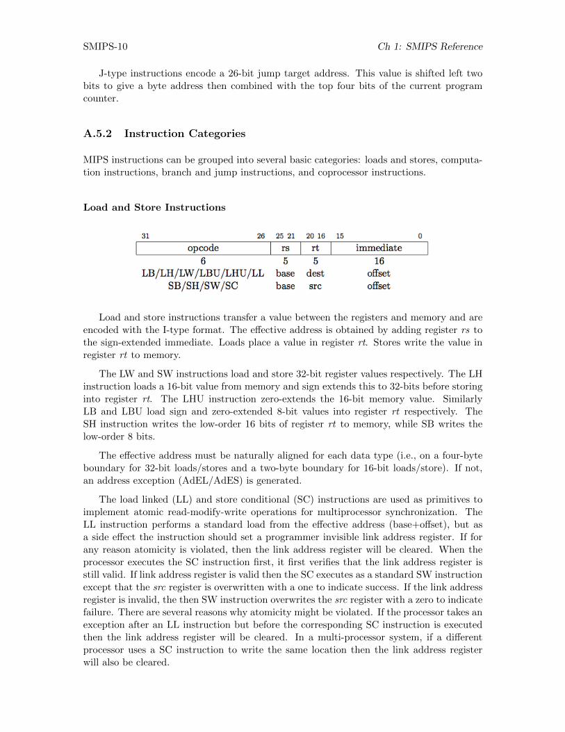
SMIPS-10 Ch 1: SMIPS Reference
J-type instructions encode a 26-bit jump target address. This value is shifted left twobits to give a byte address then combined with the top four bits of the current programcounter.
A.5.2 Instruction Categories
MIPS instructions can be grouped into several basic categories: loads and stores, computa-tion instructions, branch and jump instructions, and coprocessor instructions.
Load and Store Instructions
Load and store instructions transfer a value between the registers and memory and areencoded with the I-type format. The effective address is obtained by adding register rs tothe sign-extended immediate. Loads place a value in register rt. Stores write the value inregister rt to memory.
The LW and SW instructions load and store 32-bit register values respectively. The LHinstruction loads a 16-bit value from memory and sign extends this to 32-bits before storinginto register rt. The LHU instruction zero-extends the 16-bit memory value. SimilarlyLB and LBU load sign and zero-extended 8-bit values into register rt respectively. TheSH instruction writes the low-order 16 bits of register rt to memory, while SB writes thelow-order 8 bits.
The effective address must be naturally aligned for each data type (i.e., on a four-byteboundary for 32-bit loads/stores and a two-byte boundary for 16-bit loads/store). If not,an address exception (AdEL/AdES) is generated.
The load linked (LL) and store conditional (SC) instructions are used as primitives toimplement atomic read-modify-write operations for multiprocessor synchronization. TheLL instruction performs a standard load from the effective address (base+offset), but asa side effect the instruction should set a programmer invisible link address register. If forany reason atomicity is violated, then the link address register will be cleared. When theprocessor executes the SC instruction first, it first verifies that the link address register isstill valid. If link address register is valid then the SC executes as a standard SW instructionexcept that the src register is overwritten with a one to indicate success. If the link addressregister is invalid, the then SW instruction overwrites the src register with a zero to indicatefailure. There are several reasons why atomicity might be violated. If the processor takes anexception after an LL instruction but before the corresponding SC instruction is executedthen the link address register will be cleared. In a multi-processor system, if a differentprocessor uses a SC instruction to write the same location then the link address registerwill also be cleared.
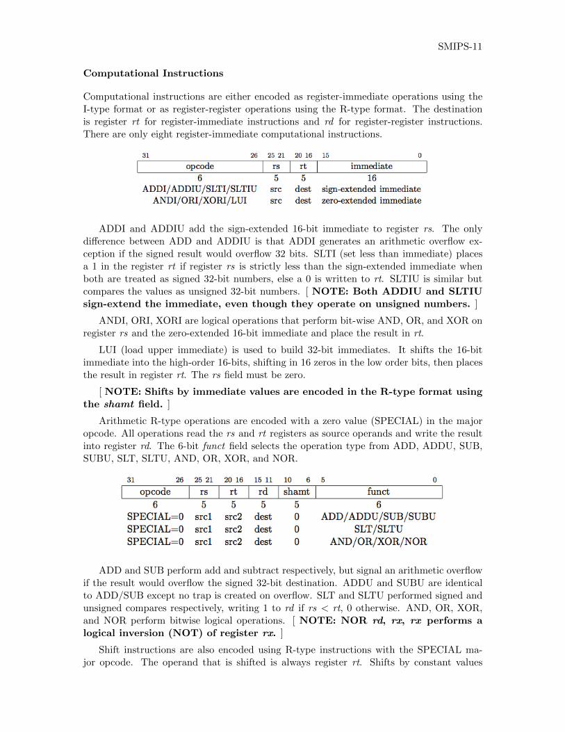
SMIPS-11
Computational Instructions
Computational instructions are either encoded as register-immediate operations using theI-type format or as register-register operations using the R-type format. The destinationis register rt for register-immediate instructions and rd for register-register instructions.There are only eight register-immediate computational instructions.
ADDI and ADDIU add the sign-extended 16-bit immediate to register rs. The onlydifference between ADD and ADDIU is that ADDI generates an arithmetic overflow ex-ception if the signed result would overflow 32 bits. SLTI (set less than immediate) placesa 1 in the register rt if register rs is strictly less than the sign-extended immediate whenboth are treated as signed 32-bit numbers, else a 0 is written to rt. SLTIU is similar butcompares the values as unsigned 32-bit numbers. [ NOTE: Both ADDIU and SLTIUsign-extend the immediate, even though they operate on unsigned numbers. ]
ANDI, ORI, XORI are logical operations that perform bit-wise AND, OR, and XOR onregister rs and the zero-extended 16-bit immediate and place the result in rt.
LUI (load upper immediate) is used to build 32-bit immediates. It shifts the 16-bitimmediate into the high-order 16-bits, shifting in 16 zeros in the low order bits, then placesthe result in register rt. The rs field must be zero.
[ NOTE: Shifts by immediate values are encoded in the R-type format usingthe shamt field. ]
Arithmetic R-type operations are encoded with a zero value (SPECIAL) in the majoropcode. All operations read the rs and rt registers as source operands and write the resultinto register rd. The 6-bit funct field selects the operation type from ADD, ADDU, SUB,SUBU, SLT, SLTU, AND, OR, XOR, and NOR.
ADD and SUB perform add and subtract respectively, but signal an arithmetic overflowif the result would overflow the signed 32-bit destination. ADDU and SUBU are identicalto ADD/SUB except no trap is created on overflow. SLT and SLTU performed signed andunsigned compares respectively, writing 1 to rd if rs < rt, 0 otherwise. AND, OR, XOR,and NOR perform bitwise logical operations. [ NOTE: NOR rd, rx, rx performs alogical inversion (NOT) of register rx. ]
Shift instructions are also encoded using R-type instructions with the SPECIAL ma-jor opcode. The operand that is shifted is always register rt. Shifts by constant values
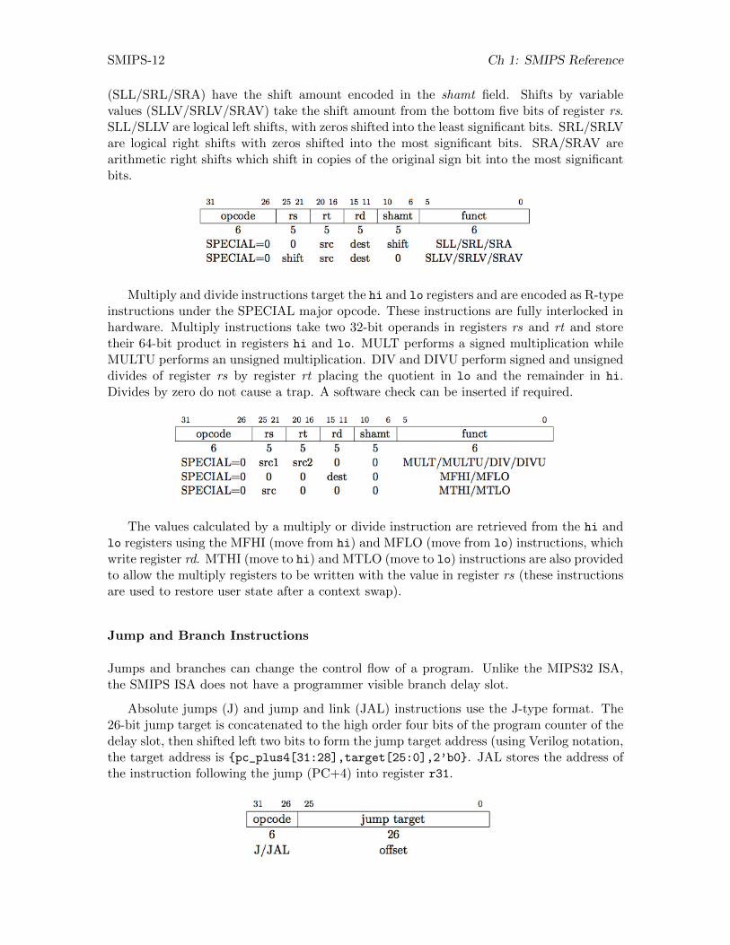
SMIPS-12 Ch 1: SMIPS Reference
(SLL/SRL/SRA) have the shift amount encoded in the shamt field. Shifts by variablevalues (SLLV/SRLV/SRAV) take the shift amount from the bottom five bits of register rs.SLL/SLLV are logical left shifts, with zeros shifted into the least significant bits. SRL/SRLVare logical right shifts with zeros shifted into the most significant bits. SRA/SRAV arearithmetic right shifts which shift in copies of the original sign bit into the most significantbits.
Multiply and divide instructions target the hi and lo registers and are encoded as R-typeinstructions under the SPECIAL major opcode. These instructions are fully interlocked inhardware. Multiply instructions take two 32-bit operands in registers rs and rt and storetheir 64-bit product in registers hi and lo. MULT performs a signed multiplication whileMULTU performs an unsigned multiplication. DIV and DIVU perform signed and unsigneddivides of register rs by register rt placing the quotient in lo and the remainder in hi.Divides by zero do not cause a trap. A software check can be inserted if required.
The values calculated by a multiply or divide instruction are retrieved from the hi andlo registers using the MFHI (move from hi) and MFLO (move from lo) instructions, whichwrite register rd. MTHI (move to hi) and MTLO (move to lo) instructions are also providedto allow the multiply registers to be written with the value in register rs (these instructionsare used to restore user state after a context swap).
Jump and Branch Instructions
Jumps and branches can change the control flow of a program. Unlike the MIPS32 ISA,the SMIPS ISA does not have a programmer visible branch delay slot.
Absolute jumps (J) and jump and link (JAL) instructions use the J-type format. The26-bit jump target is concatenated to the high order four bits of the program counter of thedelay slot, then shifted left two bits to form the jump target address (using Verilog notation,the target address is {pc_plus4[31:28],target[25:0],2’b0}. JAL stores the address ofthe instruction following the jump (PC+4) into register r31.
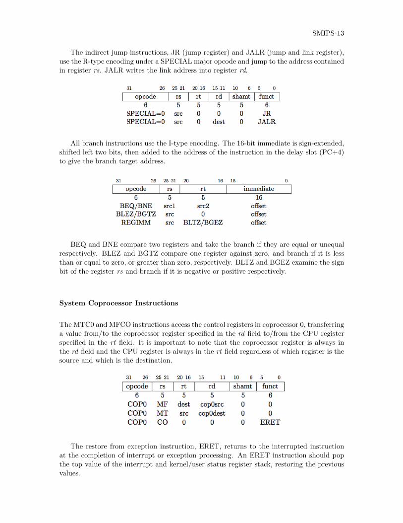
SMIPS-13
The indirect jump instructions, JR (jump register) and JALR (jump and link register),use the R-type encoding under a SPECIAL major opcode and jump to the address containedin register rs. JALR writes the link address into register rd.
All branch instructions use the I-type encoding. The 16-bit immediate is sign-extended,shifted left two bits, then added to the address of the instruction in the delay slot (PC+4)to give the branch target address.
BEQ and BNE compare two registers and take the branch if they are equal or unequalrespectively. BLEZ and BGTZ compare one register against zero, and branch if it is lessthan or equal to zero, or greater than zero, respectively. BLTZ and BGEZ examine the signbit of the register rs and branch if it is negative or positive respectively.
System Coprocessor Instructions
The MTC0 and MFCO instructions access the control registers in coprocessor 0, transferringa value from/to the coprocessor register specified in the rd field to/from the CPU registerspecified in the rt field. It is important to note that the coprocessor register is always inthe rd field and the CPU register is always in the rt field regardless of which register is thesource and which is the destination.
The restore from exception instruction, ERET, returns to the interrupted instructionat the completion of interrupt or exception processing. An ERET instruction should popthe top value of the interrupt and kernel/user status register stack, restoring the previousvalues.

SMIPS-14 Ch 1: SMIPS Reference
Coprocessor 2 Instructions
Coprocessor 2 is reserved for an implementation defined hardware unit. The MTC2 andMFC2 instructions access the registers in coprocessor 2, transferring a value from/to the co-processor register specified in the rd field to/from the CPU register specified in the rt field.The CTC2 and CFC2 instructions serve a similar process. The Coprocessor 2 implementa-tion is free to handle the coprocessor register specifiers in MTC2/MFC2 and CTC2/CFC2in any way it wishes.
The LWC2 and SWC2 instructions transfer values between memory and the coprocessorregisters. Note that although cop2dest and cop2src fields are coprocessor register specifiers,the ISA does not define how these correspond to the coprocessor register specifiers in otherCoprocessor 2 instructions.
The COP2 instruction is the primary mechanism by which a programmer can specifyinstruction bits to control Coprocessor 2. The 25-bit copfunc field is compeletely implemen-tation dependent.
Special Instructions
The SYSCALL and BREAK instructions are useful for implementing operating systems anddebuggers. The SYNC instruction can be necessary to guarantee strong load/store orderingin modern multi-processors with sophisticated memory systems.
The SYSCALL and BREAK instructions cause and immediate syscall or break excep-tion. To access the code field for use as a software parameter, the exception handler mustload the memory location containing the syscall instruction.
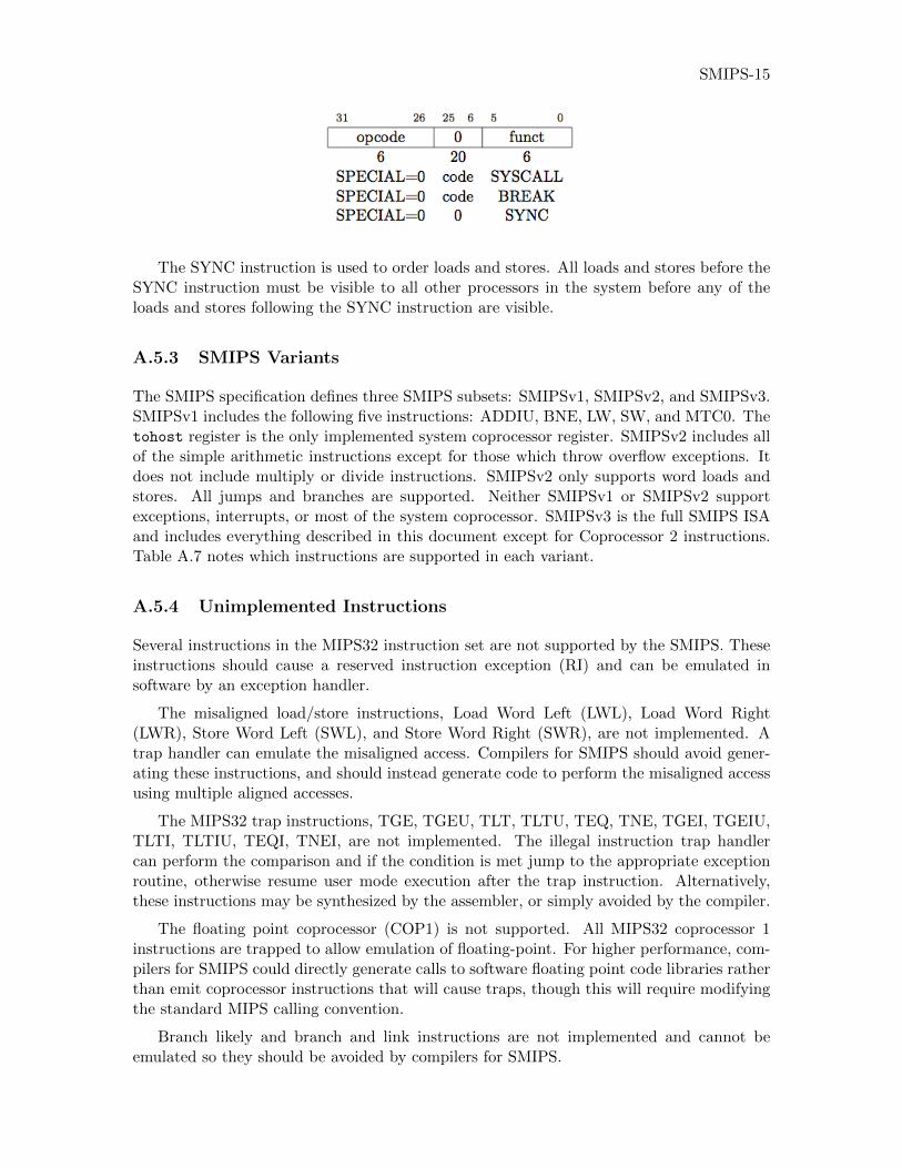
SMIPS-15
The SYNC instruction is used to order loads and stores. All loads and stores before theSYNC instruction must be visible to all other processors in the system before any of theloads and stores following the SYNC instruction are visible.
A.5.3 SMIPS Variants
The SMIPS specification defines three SMIPS subsets: SMIPSv1, SMIPSv2, and SMIPSv3.SMIPSv1 includes the following five instructions: ADDIU, BNE, LW, SW, and MTC0. Thetohost register is the only implemented system coprocessor register. SMIPSv2 includes allof the simple arithmetic instructions except for those which throw overflow exceptions. Itdoes not include multiply or divide instructions. SMIPSv2 only supports word loads andstores. All jumps and branches are supported. Neither SMIPSv1 or SMIPSv2 supportexceptions, interrupts, or most of the system coprocessor. SMIPSv3 is the full SMIPS ISAand includes everything described in this document except for Coprocessor 2 instructions.Table A.7 notes which instructions are supported in each variant.
A.5.4 Unimplemented Instructions
Several instructions in the MIPS32 instruction set are not supported by the SMIPS. Theseinstructions should cause a reserved instruction exception (RI) and can be emulated insoftware by an exception handler.
The misaligned load/store instructions, Load Word Left (LWL), Load Word Right(LWR), Store Word Left (SWL), and Store Word Right (SWR), are not implemented. Atrap handler can emulate the misaligned access. Compilers for SMIPS should avoid gener-ating these instructions, and should instead generate code to perform the misaligned accessusing multiple aligned accesses.
The MIPS32 trap instructions, TGE, TGEU, TLT, TLTU, TEQ, TNE, TGEI, TGEIU,TLTI, TLTIU, TEQI, TNEI, are not implemented. The illegal instruction trap handlercan perform the comparison and if the condition is met jump to the appropriate exceptionroutine, otherwise resume user mode execution after the trap instruction. Alternatively,these instructions may be synthesized by the assembler, or simply avoided by the compiler.
The floating point coprocessor (COP1) is not supported. All MIPS32 coprocessor 1instructions are trapped to allow emulation of floating-point. For higher performance, com-pilers for SMIPS could directly generate calls to software floating point code libraries ratherthan emit coprocessor instructions that will cause traps, though this will require modifyingthe standard MIPS calling convention.
Branch likely and branch and link instructions are not implemented and cannot beemulated so they should be avoided by compilers for SMIPS.
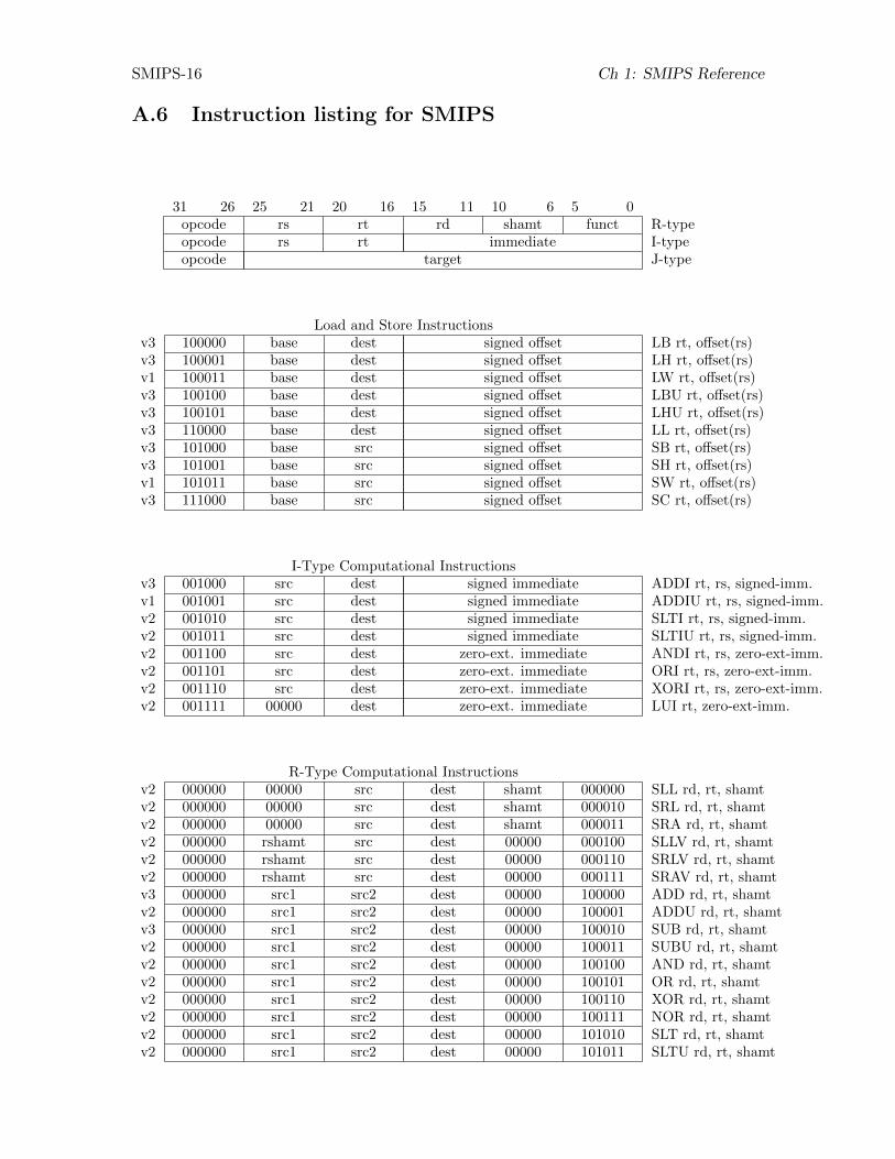
SMIPS-16 Ch 1: SMIPS Reference
A.6 Instruction listing for SMIPS
31 26 25 21 20 16 15 11 10 6 5 0opcode rs rt rd shamt funct R-typeopcode rs rt immediate I-typeopcode target J-type
Load and Store Instructionsv3 100000 base dest signed offset LB rt, offset(rs)v3 100001 base dest signed offset LH rt, offset(rs)v1 100011 base dest signed offset LW rt, offset(rs)v3 100100 base dest signed offset LBU rt, offset(rs)v3 100101 base dest signed offset LHU rt, offset(rs)v3 110000 base dest signed offset LL rt, offset(rs)v3 101000 base src signed offset SB rt, offset(rs)v3 101001 base src signed offset SH rt, offset(rs)v1 101011 base src signed offset SW rt, offset(rs)v3 111000 base src signed offset SC rt, offset(rs)
I-Type Computational Instructionsv3 001000 src dest signed immediate ADDI rt, rs, signed-imm.v1 001001 src dest signed immediate ADDIU rt, rs, signed-imm.v2 001010 src dest signed immediate SLTI rt, rs, signed-imm.v2 001011 src dest signed immediate SLTIU rt, rs, signed-imm.v2 001100 src dest zero-ext. immediate ANDI rt, rs, zero-ext-imm.v2 001101 src dest zero-ext. immediate ORI rt, rs, zero-ext-imm.v2 001110 src dest zero-ext. immediate XORI rt, rs, zero-ext-imm.v2 001111 00000 dest zero-ext. immediate LUI rt, zero-ext-imm.
R-Type Computational Instructionsv2 000000 00000 src dest shamt 000000 SLL rd, rt, shamtv2 000000 00000 src dest shamt 000010 SRL rd, rt, shamtv2 000000 00000 src dest shamt 000011 SRA rd, rt, shamtv2 000000 rshamt src dest 00000 000100 SLLV rd, rt, shamtv2 000000 rshamt src dest 00000 000110 SRLV rd, rt, shamtv2 000000 rshamt src dest 00000 000111 SRAV rd, rt, shamtv3 000000 src1 src2 dest 00000 100000 ADD rd, rt, shamtv2 000000 src1 src2 dest 00000 100001 ADDU rd, rt, shamtv3 000000 src1 src2 dest 00000 100010 SUB rd, rt, shamtv2 000000 src1 src2 dest 00000 100011 SUBU rd, rt, shamtv2 000000 src1 src2 dest 00000 100100 AND rd, rt, shamtv2 000000 src1 src2 dest 00000 100101 OR rd, rt, shamtv2 000000 src1 src2 dest 00000 100110 XOR rd, rt, shamtv2 000000 src1 src2 dest 00000 100111 NOR rd, rt, shamtv2 000000 src1 src2 dest 00000 101010 SLT rd, rt, shamtv2 000000 src1 src2 dest 00000 101011 SLTU rd, rt, shamt
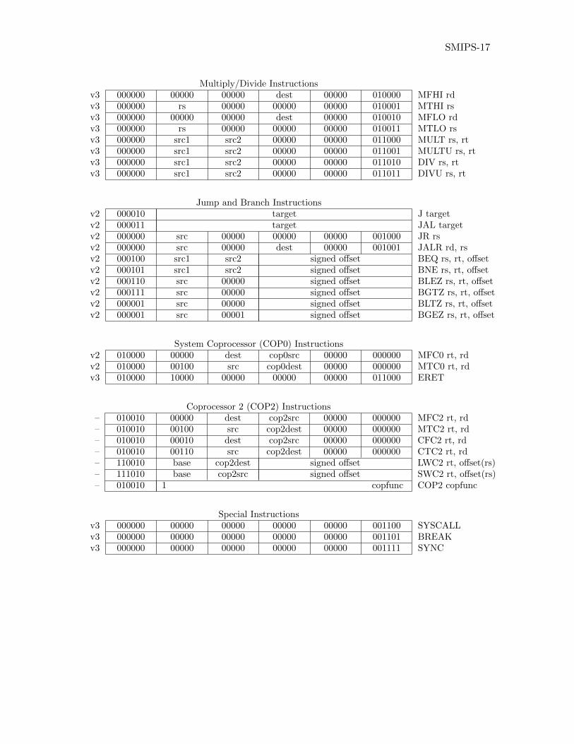
SMIPS-17
Multiply/Divide Instructionsv3 000000 00000 00000 dest 00000 010000 MFHI rdv3 000000 rs 00000 00000 00000 010001 MTHI rsv3 000000 00000 00000 dest 00000 010010 MFLO rdv3 000000 rs 00000 00000 00000 010011 MTLO rsv3 000000 src1 src2 00000 00000 011000 MULT rs, rtv3 000000 src1 src2 00000 00000 011001 MULTU rs, rtv3 000000 src1 src2 00000 00000 011010 DIV rs, rtv3 000000 src1 src2 00000 00000 011011 DIVU rs, rt
Jump and Branch Instructionsv2 000010 target J targetv2 000011 target JAL targetv2 000000 src 00000 00000 00000 001000 JR rsv2 000000 src 00000 dest 00000 001001 JALR rd, rsv2 000100 src1 src2 signed offset BEQ rs, rt, offsetv2 000101 src1 src2 signed offset BNE rs, rt, offsetv2 000110 src 00000 signed offset BLEZ rs, rt, offsetv2 000111 src 00000 signed offset BGTZ rs, rt, offsetv2 000001 src 00000 signed offset BLTZ rs, rt, offsetv2 000001 src 00001 signed offset BGEZ rs, rt, offset
System Coprocessor (COP0) Instructionsv2 010000 00000 dest cop0src 00000 000000 MFC0 rt, rdv2 010000 00100 src cop0dest 00000 000000 MTC0 rt, rdv3 010000 10000 00000 00000 00000 011000 ERET
Coprocessor 2 (COP2) Instructions– 010010 00000 dest cop2src 00000 000000 MFC2 rt, rd– 010010 00100 src cop2dest 00000 000000 MTC2 rt, rd– 010010 00010 dest cop2src 00000 000000 CFC2 rt, rd– 010010 00110 src cop2dest 00000 000000 CTC2 rt, rd– 110010 base cop2dest signed offset LWC2 rt, offset(rs)– 111010 base cop2src signed offset SWC2 rt, offset(rs)– 010010 1 copfunc COP2 copfunc
Special Instructionsv3 000000 00000 00000 00000 00000 001100 SYSCALLv3 000000 00000 00000 00000 00000 001101 BREAKv3 000000 00000 00000 00000 00000 001111 SYNC
Bibliography
[1] Bluespec, Inc. BluespecTM SystemVerilog Version Reference Guide, 2010.
[2] Bluespec, Inc. BluespecTM SystemVerilog Version User Guide, 2010.
[3] J. L. Hennessy and D. Patterson. Computer Organization and Design: The Hardware/SoftwareInterface (Second Edition). Morgan Kaufmann, February 1997. ISBN 1558604286.
[4] J. L. Hennessy and D. A. Patterson. Computer Architecture: A Quantitative Approach (FifthEdition). Morgan Kaufman, September 2011.
[5] M. T. Inc. MIPS32 Architecture for Programmers. 2002.http://www.mips.com/publications/processor architecture.html.
[6] G. Kane and J. Heinrich. MIPS RISC Architecture (2nd edition). Prentice Hall, September 1991.ISBN 0135904722.
[7] R. S. Nikhil and K. R. Czeck. BSV by Example. CreateSpace, December 2010. ISBN-10:1456418467; ISBN-13: 978-1456418465; avail: Amazon.com.
[8] D. Sweetman. See MIPS Run. Morgan Kaufmann, April 1999. ISBN 1558604103.
BIB-1